Compressed sensing of block-sparse positive vectors
Abstract
In this paper we revisit one of the classical problems of compressed sensing. Namely, we consider linear under-determined systems with sparse solutions. A substantial success in mathematical characterization of an optimization technique typically used for solving such systems has been achieved during the last decade. Seminal works [4, 18] showed that the can recover a so-called linear sparsity (i.e. solve systems even when the solution has a sparsity linearly proportional to the length of the unknown vector). Later considerations [14, 13] (as well as our own ones [55, 51]) provided the precise characterization of this linearity. In this paper we consider the so-called structured version of the above sparsity driven problem. Namely, we view a special case of sparse solutions, the so-called block-sparse solutions. Typically one employs -optimization as a variant of the standard to handle block-sparse case of sparse solution systems. We considered systems with block-sparse solutions in a series of work [52, 46, 54, 58] where we were able to provide precise performance characterizations if the -optimization similar to those obtained for the standard optimization in [55, 51]. Here we look at a similar class of systems where on top of being block-sparse the unknown vectors are also known to have components of the same sign. In this paper we slightly adjust -optimization to account for the known signs and provide a precise performance characterization of such an adjustment.
Index Terms: Compressed sensing; optimization; linear systems of equations; signed unknown vectors.
1 Introduction
As usual we start by recalling on the basic mathematical definitions related to under-determined systems of linear equations. These problems are one of the mathematical cornerstones of compressed sensing (of course a great deal of work has been done in the compressed sensing; instead of reviewing it here we, for more on compressed sensing ideas, refer to the introductory papers [4, 18]). Since this paper will be dealing with certain mathematical aspects of compressed sensing under-determined systems of linear equations will be its a focal point.
To insure that we are on a right mathematical track we will along these lines start with providing their an as simple as possible description. One typically starts with a systems matrix which is an () dimensional matrix with real entries and then considers an dimensional vector that also has real entries but on top of that no more than nonzero entries (in the rest of this paper we will call such a vector -sparse). Then one forms the product of and to obtain
| (1) |
Clearly, in general is an dimensional vector with real entries. Then, for a moment one pretends that is not known and poses the following inverse problem: given and from (1) can one then determine ? Or in other words, can one for a given pair and find the sparse solution of the following linear systems of equation type of problem (see, Figure 1)
| (2) |

Of course, based on (1) such an exists (moreover, it is an easy algebraic exercise to show that when it is in fact unique). Additionally, we will assume that there is no in (2) that is less than sparse. One often (especially within the compressed sensing context) rewrites the problem described above (and given in (2)) in the following way
| min | |||||
| subject to | (3) |
where is what is typically called norm of vector . For all practical purposes we will view as the number that counts how many nonzero entries has.
To make writing in the rest of the paper easier, we will assume the so-called linear regime, i.e. we will assume that and that the number of equations is where and are constants independent of (more on the non-linear regime, i.e. on the regime when is larger than linearly proportional to can be found in e.g. [9, 27, 28]). Of course, we do mention that all of our results can easily be adapted to various nonlinear regimes as well.
Looking back at (2), clearly one can consider an exhaustive search type of solution where one would look at all subsets of columns of and then attempt to solve the resulting system. However, in the linear regime that we assumed above such an approach becomes prohibitively slow as grows. That of course led in last several decades towards a search for more clever algorithms for solving (2). Many great algorithms were developed (especially during the last decade) and many of them have even provably excellent performance measures (see, e.g. [62, 64, 37, 20, 36, 11, 15]).
A particularly successful technique for solving (2) that will be of our interest in this paper is a linear programming relaxation of (3), called -optimization. (Variations of the standard -optimization from e.g. [5, 8, 42]) as well as those from [41, 25, 30, 31, 32, 12, 50, 44] related to -optimization, are possible as well.) Basic -optimization algorithm finds in (2) or (3) by solving the following -norm minimization problem
| min | |||||
| subject to | (4) |
Due to its popularity the literature on the use of the above algorithm is rapidly growing. Surveying it here goes way beyond the main interest of this paper and we defer doing so to a review paper. Here we just briefly mention that in seminal works [4, 18] it was proven in a statistical context that for any there will be a such that is the solution of (4). [14, 13] (later our own work [55, 51] as well) for any determined the exact values of such that almost any is the solution of (4). That essentially settled a statistical performance characterization of (4) when employed as an alternate to (3).
Theorem 1.
(Exact threshold) Let be an matrix in (2) with i.i.d. standard normal components. Let the unknown in (2) be -sparse. Further, let the location and signs of nonzero elements of be arbitrarily chosen but fixed. Let be large and let and be constants independent of and . Let erfinv be the inverse of the standard error function associated with zero-mean unit variance Gaussian random variable. Further, let and satisfy the following:
Fundamental characterization of the performance:
-
| (5) |
Proof.
As mentioned above, the above theorem (as well as corresponding results obtained earlier in [14, 13])) essentially settled typical behavior of optimization when used for solving (2) or (3). In this paper we will look at a problem similar to the one from (3) (or (2)). Namely, we will view problem from (2)) within the following framework: we will assume that is not only sparse but also what is called block-sparse. Such an assumption can then be incorporated in the recovery algorithm as well. Before proceeding further with the presentation of such an algorithm we briefly sketch how the rest of the paper will be organized. In Section 2 we first introduce the block-sparse vectors and their a special variant that we will call positive block-sparse vectors. In Section 3 we then present a performance analysis of an algorithm that can be used for solving linear under-determined systems known to have positive block-sparse solutions. Finally, in Sections 4 we discuss obtained results and provide a few conclusions.
2 Block-sparse positive vectors
What we described in the previous section assumes solving an under-determined system of linear equations with a standard restriction that the solution vector is sparse. Sometimes one may however encounter applications when the unknown in addition to being sparse has a certain structure as well. The so-called block-sparse vectors are such a type of vectors and will be the main subject of this paper. These vectors and their potential applications and recovery algorithms were investigated to a great detail in a series of recent references (see e.g. [21, 22, 60, 39, 23, 1, 54, 58, 26, 6]). A related problem of recovering jointly sparse vectors and its applications were also considered to a great detail in e.g. [69, 70, 63, 2, 7, 10, 35, 61, 66, 65, 24, 3, 38] and many references therein. While various other structures as well as their applications gained significant interest over last few years we here refrain from describing them into fine details and instead refer to nice work of e.g. [33, 68, 34, 40, 59]. Since we will be interested in characterizing mathematical properties of solving linear systems that are similar to many of those mentioned above we just state here in brief that from a mathematical point of view in all these cases one attempts to improve the recoverability potential of the standard algorithms (which are typically similar to the one described in the previous section) by incorporating the knowledge of the unknown vector structure.
To get things started we first introduce the block-sparse vectors. The subsequent exposition will also be somewhat less cumbersome if we assume that integers and are chosen such that is an integer and it represents the total number of blocks that consists of. Clearly is the length of each block. Furthermore, we will assume that is an integer as well and that , are the blocks of (see Figure 2).
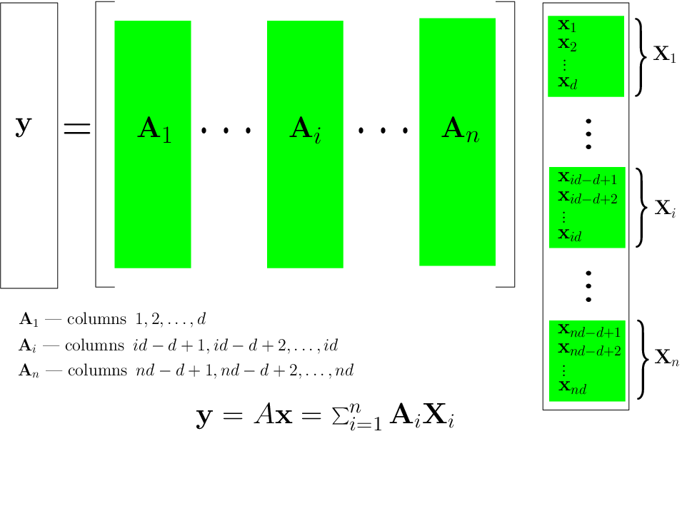
Then we will call any signal k-block-sparse if its at most blocks are non-zero (non-zero block is a block that is not a zero block; zero block is a block that has all elements equal to zero). Since -block-sparse signals are -sparse one could then use (4) to recover the solution of (2). While this is possible, it clearly uses the block structure of in no way. There are of course many ways how one can attempt to exploit the block-sparse structure. Below we just briefly mentioned a few of them.
A few approaches from a vast literature cited above have recently attracted significant amount of attention. The first thing one can think of when facing the block-structured unknown vectors is how to extend results known in the non-block (i.e. standard) case. In [63] the standard OMP (orthogonal matching pursuit) was generalized so that it can handle the jointly-sparse vectors more efficiently and improvements over the standard OMP were demonstrated. In [1, 23] algorithms similar to the one from this paper were considered. It was explicitly shown through the block-RIP (block-restricted isometry property) type of analysis (which essentially extends to the block case the concepts introduced in [4] for the non-block scenario) that one can achieve improvements in recoverable thresholds compared to the non-block case. Also, important results were obtained in [24] where it was shown (also through the block-RIP type of analysis) that if one considers average case recovery of jointly-sparse signals the improvements in recoverable thresholds over the standard non-block signals are possible (of course, trivially, jointly-sparse recovery offers no improvement over the standard non-block scenario in the worst case). All these results provided a rather substantial basis for belief that the block-sparse recovery can provably be significantly more successful than the standard non-block one.
To exploit the block structure of in [60] the following polynomial-time algorithm (essentially a combination of and optimizations) was considered (see also e.g. [70, 69, 1, 22, 65])
| min | |||||
| subject to | (6) |
Extensive simulations in [60] demonstrated that as grows the algorithm in (6) significantly outperforms the standard . The following was shown in [60] as well: let be an matrix with a basis of null-space comprised of i.i.d. Gaussian elements; if then there is a constant such that all -block-sparse signals with sparsity , can be recovered with overwhelming probability by solving (6). The precise relation between and how fast and was quantified in [60] as well. In [54, 58] we extended the results from [60] and obtained the values of the recoverable block-sparsity for any , i.e. for . More precisely, for any given constant we in [54, 58] determined a constant such that for a sufficiently large (6) with overwhelming probability recovers any -block-sparse signal with sparsity less then . (Under overwhelming probability we in this paper assume a probability that is no more than a number exponentially decaying in away from .)
Clearly, for any given constant there is a maximum allowable value of such that for any given -sparse in (2) the solution of (6) is with overwhelming probability exactly that given -sparse . This value of is typically referred to as the strong threshold (see [14, 52]). Similarly, for any given constant and any given with a given fixed location and a given fixed directions of non-zero blocks there will be a maximum allowable value of such that (6) finds that given in (2) with overwhelming probability. We will refer to this maximum allowable value of as the weak threshold and will denote it by (see, e.g. [53, 55]).
While [54, 58] provided fairly sharp strong threshold values they had done so in a somewhat asymptotic sense. Namely, the analysis presented in [54, 58] assumed fairly large values of block-length . As such the analysis in [54, 58] then provided an ultimate performance limit of -optimization rather than its performance characterization as a function of a particular fixed block-length.
In our own work [52] we extended the results of [54, 58] and provided a novel probabilistic framework for performance characterization of (6) through which we were finally able to view block-length as a parameter of the system (the heart of the framework was actually introduced in [55] and it seemed rather powerful; in fact, we afterwards found hardly any sparse type of problem that the framework was not able to handle with an almost impeccable precision). Using the framework we obtained lower bounds on . These lower bounds were in an excellent numerical agreement with the values obtained for through numerical simulations. In a followup [46] we then showed that the lower bounds on obtained in [52] are actually exact.
The following theorem essentially summarizes the results obtained in [52, 46] and effectively establishes for any the exact value of for which (6) finds the -block-sparse from (2).
Theorem 2.
([52, 46] Exact weak threshold; block-sparse ) Let be an matrix in (2) with i.i.d. standard normal components. Let the unknown in (2) be -block-sparse with the length of its blocks . Further, let the location and the directions of nonzero blocks of be arbitrarily chosen but fixed. Let be large and let and be constants independent of and . Let and be the incomplete gamma function and its inverse, respectively. Further, let all ’s below be arbitrarily small constants.
- 1.
- 2.
As we mentioned above, the block-sparse structure is clearly not the only one that can be imposed on the unknown . Among the most typical ones usually considered in parallel with the standard sparse scenario is what is called the case of signed (say positive-nonnegative/negative-nonpositive) vectors . Such vectors can find applications in scenarios when the physics of the problem does not allow for different signs of the components of . Also, they have been of interest for a long time from a purely mathematical point of view (see, e.g. [17, 16, 55, 51, 53, 57]). In scenarios when it is known that all components of are of the same sign (say positive) one typically replaces (4) with the following
| min | |||||
| subject to | (11) | ||||
As mentioned above, in [55, 51] we showed how one characterize the performance of (11). In this paper we look at the above mentioned block-sparse vectors that are also signed (say positive). In such scenarios one can use the following modification of (6)
| min | |||||
| subject to | (12) | ||||
Of course, (12) relates to (6) in the same way (11) relates to (4). As analysis of [55, 51] showed one can achieve a higher recoverable sparsity when components of are a priori known to be say positive (i.e. of the same sign). This of course is not surprising since one would naturally expect that the more available information about unknown the easier its recovery. Along the same lines, one can then expect that a similar phenomenon should occur when one is dealing with the block-sparse signals. Among other things, the analysis that we will present below will confirm such an expectation. Of course, the key feature of what will present below will be a precise performance analysis of (12) when used for recovery of positive block-sparse vectors in (2).
3 Performance analysis of (12)
In this section we will attempt to obtain the results qualitatively similar to those presented in Theorems 1 and 2. Of course, the results presented in Theorems 1 and 2 are related to performance of (4) and (6), respectively, whereas here we will try to create their an analogue that relates to (12). As mentioned earlier, the results presented in Theorems 1 and 2 were obtained in a series of work [53, 55, 51, 52, 46]. Below, we adapt some of these results so that they can handle the problems of interest here. In doing so, we will in this and all subsequent sections assume a substantial level of familiarity with many of the well-known results that relate to the performance characterization of (4) and (6) (we will fairly often recall on many results/definitions that we established in [53, 55, 51, 52, 46]).
Before proceeding further with a detail presentation we briefly sketch what specifically we will be interested in showing below. Namely, using the analysis of [55, 51, 52, 46] mentioned earlier, for a specific group of randomly generated matrices , one can determine values for the entire range of , i.e. for , where is the maximum allowable value of such that (12) finds the positive -block-sparse solution of (2) with overwhelming probability for any -block-sparse with given a fixed location and a fixed combination of directions of nonzero blocks, and a priori known to have non-negative components. (As mentioned earlier and discussed to great extent in [57, 53, 55, 51, 52, 46], this value of is often referred to as the weak threshold.)
We are now ready to start the analysis. We begin by recalling on a theorem from [46] that provides a characterization as to when the solution of (12) is , i.e. the positive -block-sparse solution of (2) or (3). Since the analysis will clearly be irrelevant with respect to what particular location and what particular combination of directions of nonzero blocks are chosen, we can for the simplicity of the exposition and without a loss of generality assume that the blocks of are equal to zero and the blocks of have fixed directions. Also, as mentioned above, we will assume that all components of are non-negative, i.e. . Under these assumptions we have the following theorem (similar characterizations adopted in various contexts can be found in [19, 67, 60, 53, 30, 52, 46, 56, 54]).
Theorem 3.
([52, 46, 56] Nonzero part of has fixed directions and location) Assume that an matrix is given. Let be a positive -block-sparse vector from . Also let and let the directions of vectors be fixed. Further, assume that and that is an vector with blocks , defined in a way analogous to the definition of blocks . If
| (13) |
then the solution of (6) is . Moreover, if
| (14) |
then there will be a positive -block-sparse from the above defined set that satisfies (2) and is not the solution of (12).
Proof.
Having matrix such that (13) holds would be enough for solutions of (12) and (3) (or (2)) to coincide. If one assumes that and are proportional to (the case of our interest in this paper) then the construction of the deterministic matrices that would satisfy (13) is not an easy task (in fact, one may say that together with the ones that correspond to the standard it is one of the most fundamental open problems in the area of theoretical compressed sensing). However, turning to random matrices significantly simplifies things. That is the route that will pursuit below. In fact to be a bit more specific, we will assume that the elements of matrix are i.i.d. standard normal random variables. All results that we will present below will hold for many other types of randomness (we will comment on this in more detail in Section 4). However, to make the presentation as smooth as possible we assume the standard Gaussian scenario.
Theorem 4.
([29] Escape through a mesh) Let be a subset of the unit Euclidean sphere in . Let be a random -dimensional subspace of , distributed uniformly in the Grassmanian with respect to the Haar measure. Let
| (15) |
where is a random column vector in with i.i.d. components. Assume that . Then
| (16) |
As mentioned above, to make use of Theorem 4 we follow the strategy presented in [55, 52]. We start by defining a set
| (17) |
and
| (18) |
where as earlier is a random column vector in with i.i.d. components and is the unit -dimensional sphere. Let , and let be the orthogonal matrices such that . Set
| (19) |
and
| (20) |
Since and have the same distribution we have . The strategy of [55, 52] assumes roughly the following: if is positive with overwhelming probability for certain combination of , , and then for one has a lower bound on the true value of the weak threshold with overwhelming probability (we recall that as usual under overwhelming probability we of course assume a probability that is no more than a number exponentially decaying in away from ). The above basically means that if one can handle then, when is large one can, roughly speaking, use the condition to obtain an attainable lower bound for any given .
To that end we then look at
| (21) |
where to make writing simpler we have replaced the from (20) with a . Let
| (22) |
Also set
Following further what was done in [55, 52] one then can write
| (23) |
Set and let be the -th element in the sequence of elements of sorted in increasing order. Set
| (24) |
Let . Then one can simplify (23) in the following way
| subject to | (25) | ||||
where is the -th element of . Let be a vector such that , , and .
Following step by step the derivation in [55, 52] one has, based on the Lagrange duality theory, that there is a such that
where we recall that is the -th element of vector . Moreover, [55] also establishes the way to determine a critical . Roughly speaking it establishes the following identity
| (27) |
To make the above results operational one would have to estimate the expectations that they contain. [55, 52] established a technique powerful enough to do so. However, differently from [55, 52] one has to be fairly careful when it comes to the distributions of the underlying random quantities. While the corresponding ones in [55, 52] were relatively simple the ones that we face here are a bit harder to analytically quantify. We, hence present these considerations in a separate section below.
3.1 Explicit characterization of
We separately characterize all of the quantities needed for characterization of .
3.1.1 Explicit characterization of
3.1.2 Explicit characterization of
3.1.3 Explicit characterization of
We start with the following line of identities
| (34) | |||||
Following further what was done in [55, 52] one has
| (35) |
A combination of (34) and (35) gives
| (36) |
We summarize the above results in the following theorem.
Theorem 5.
(Exact weak threshold) Let be a measurement matrix in (2) with the null-space uniformly distributed in the Grassmanian. Let the unknown in (2) be positive -block-sparse with the length of its blocks . Further, let the location and the directions of nonzero blocks of be arbitrarily chosen but fixed. Let be large and let and be constants independent of and . Let and be the incomplete gamma function and its inverse, respectively. Further, let be the following function
| (37) |
and let be its inverse. Let , () be the solution of
| (38) |
- 1.
- 2.
Proof.
Remark: To make writing easier in the previous theorem we removed all ’s used in Theorem 2 and typically used in [55, 52, 51, 46].
The above theorem essentially settles typical behavior of the optimization from (12) when used for solving (2) or (3) assuming that is a priori known to be positive and block-sparse.
The results for the weak threshold obtained from the above theorem are presented in Figure 3. More precisely, on the left hand side of Figure 3 we present the results that can be obtained from Theorem 5. In addition to that we on the right hand side of Figure 3 present the results one can obtain using Theorem 2. As is expected, given that the positive case assumes a bit more knowledge about the recovery abilities of an algorithm (namely, in this case the one given in (12)) tailored for such a case are a bit higher.


To get a feeling how accurately the presented analysis portraits the real behavior of the analyzed algorithms we below present a small set of results we obtained through numerical experiments.
3.2 Numerical experiments
In this section we briefly discuss the results that we obtained from numerical experiments. In our numerical experiments we fixed and when On the other hand to get a bit of a finer resolution we set when . We then generated matrices of size with . The components of the measurement matrices were generated as i.i.d. zero-mean unit variance Gaussian random variables. For each we generated randomly -block-sparse positive signals for several different values of from the transition zone (the locations of non-zero elements of were chosen randomly as well). For each combination we generated different problem instances and recorded the number of times the -optimization algorithm from (12) failed to recover the correct -block-sparse positive . The obtained data are then interpolated and graphically presented on the right hand side of Figure 4. The color of any point shows the probability of having -optimization from (12) succeed for a combination that corresponds to that point. The colors are mapped to probabilities according to the scale on the right hand side of the figure. The simulated results can naturally be compared to the theoretical prediction from Theorem 5. Hence, we also show on the right hand side the theoretical value for the threshold calculated according to Theorem 5 (and obviously shown on the left hand side of the figure as well). We observe that the simulation results are in a good agreement with the theoretical calculation.

3.3 – weak threshold
When the block length is large one can simplify the conditions for finding the thresholds obtained in the previous section. Hence, in this section we establish weak thresholds when , i.e. we establish ultimate benefit of -optimization from (12) when used in recovery of block-sparse positive vectors from (2). Throughout this section we choose in order to simplify the exposition.
Following the reasoning presented in [52] it is not that difficult to see that choosing in (39) would provide a valid threshold condition as well (in general is not optimal for a fixed value , i.e. when is not large a better choice for is the one given in Theorem 5). However it can be shown that the choice gives us the following corollary of Theorem 5.
Corollary 1.
() Let be a measurement matrix in (2) with the null-space uniformly distributed in the Grassmanian. Let the unknown in (2) be positive -block-sparse with the length of its blocks . Further, let the location and the directions of nonzero blocks of be arbitrarily chosen but fixed. Let be large and let and be constants independent of and . Assume that is independent of . If and satisfy
| (41) |
then the solution of (12) is with overwhelming probability the positive -block sparse in (2).
Proof.
The results for the weak threshold obtained in the above corollary are shown in figures in earlier sections as curves denoted by .
4 Conclusion
In this paper we studied a variant of the standard compressed sensing setup. The variant that we studied assumes vectors that are sparse but also structured. The type of structure that we studied is the co-called block-sparsity. While the standard block-sparsity has been studied in [52, 46] here we combine it with another type of structure, that accounts for a priori known (same) signs of unknown vectors.
Typically when the unknown vectors are block-sparse one handles them by employing an norm combination in place of the standard norm. We looked at a signed modification of norm and analyzed how it fares when used for recovery of block-sparse signed vectors from an under-determined system of linear equations. The analysis we provided viewed linear systems in a statistical context. For such systems we then established a precise probabilistic characterization of problem dimensions for which the signed modification of norm is guaranteed to recover with overwhelming probability the block-sparsest positive unknown vector.
As was the case with many results we developed (see, e.g. [55, 45, 43, 49]), the purely theoretical results we presented in this paper are valid for the so-called Gaussian models, i.e. for systems with i.i.d. Gaussian coefficients. Such an assumption significantly simplified our exposition. However, all results that we presented can easily be extended to the case of many other models of randomness. There are many ways how this can be done. Instead of recalling on them here we refer to a brief discussion about it that we presented in [45, 43].
As for usefulness of the presented results, similarly to many of the results we created within compressed sensing, there is hardly any limit. One can look at a host of related problems from the compressed sensing literature. These include for example, all noisy variations, approximately sparse unknown vectors, vectors with a priori known structure (block-sparse, binary/box constrained etc.), all types of low rank matrix recoveries, various other algorithms like -optimization, SOCP’s, LASSO’s, and many, many others. Each of these problems has its own specificities and adapting the methodology presented here usually takes a bit of work but in our view is now a routine. While we will present some of these applications we should emphasize that their contribution will be purely on an application level.
References
- [1] R. Baraniuk, V. Cevher, M. Duarte, and C. Hegde. Model-based compressive sensing. available online at http://www.dsp.ece.rice.edu/cs/.
- [2] D. Baron, M. Wakin, M. Duarte, S. Sarvotham, and Richard Baraniuk. Distributed compressed sensing. Allerton, 2005.
- [3] T. Blumensath and M. E. Davies. Sampling theorems for signals from the union of finite-dimensional linear subspaces. IEEE Transactions on Information Theory, 55(4):187–1882, 2009.
- [4] E. Candes, J. Romberg, and T. Tao. Robust uncertainty principles: exact signal reconstruction from highly incomplete frequency information. IEEE Trans. on Information Theory, 52:489–509, December 2006.
- [5] E. Candes, M. Wakin, and S. Boyd. Enhancing sparsity by reweighted l1 minimization. J. Fourier Anal. Appl., 14:877–905, 2008.
- [6] V. Cevher, P. Indyk, C. Hegde, and R. G. Baraniuk. Recovery of clustered sparse signals from compressive measurements. SAMPTA, International Conference on Sampling Theory and Applications, 2009. Marseille, France.
- [7] J. Chen and X. Huo. Theoretical results on sparse representations of multiple-measurement vectors. IEEE Trans. on Signal Processing, Dec 2006.
- [8] S. Chretien. An alternating ell-1 approach to the compressed sensing problem. 2008. available online at http://www.dsp.ece.rice.edu/cs/.
- [9] G. Cormode and S. Muthukrishnan. Combinatorial algorithms for compressed sensing. SIROCCO, 13th Colloquium on Structural Information and Communication Complexity, pages 280–294, 2006.
- [10] S. Cotter, B. Rao, K. Engan, and K. Kreutz-Delgado. Sparse solutions to linear inverse problems with multiple measurement vectors. IEEE Trans. on Signal Porcessing, July 2005.
- [11] W. Dai and O. Milenkovic. Subspace pursuit for compressive sensing signal reconstruction. Preprint, page available at arXiv:0803.0811, March 2008.
- [12] M. E. Davies and R. Gribonval. Restricted isometry constants where ell-p sparse recovery can fail for . available online at http://www.dsp.ece.rice.edu/cs/.
- [13] D. Donoho. Neighborly polytopes and sparse solutions of underdetermined linear equations. 2004. Technical report, Department of Statistics, Stanford University.
- [14] D. Donoho. High-dimensional centrally symmetric polytopes with neighborlines proportional to dimension. Disc. Comput. Geometry, 35(4):617–652, 2006.
- [15] D. Donoho, A. Maleki, and A. Montanari. Message-passing algorithms for compressed sensing. Proc. National Academy of Sciences, 106(45):18914–18919, Nov. 2009.
- [16] D. Donoho and J. Tanner. Neighborliness of randomly-projected simplices in high dimensions. Proc. National Academy of Sciences, 102(27):9452–9457, 2005.
- [17] D. Donoho and J. Tanner. Sparse nonnegative solutions of underdetermined linear equations by linear programming. Proc. National Academy of Sciences, 102(27):9446–9451, 2005.
- [18] D. L. Donoho. Compressed sensing. IEEE Trans. on Information Theory, 52(4):1289–1306, 2006.
- [19] D. L. Donoho and X. Huo. Uncertainty principles and ideal atomic decompositions. IEEE Trans. Inform. Theory, 47(7):2845–2862, November 2001.
- [20] D. L. Donoho, Y. Tsaig, I. Drori, and J.L. Starck. Sparse solution of underdetermined linear equations by stagewise orthogonal matching pursuit. 2007. available online at http://www.dsp.ece.rice.edu/cs/.
- [21] Y. C. Eldar and H. Bolcskei. Block-sparsity: Coherence and efficient recovery. ICASSP, International Conference on Acoustics, Signal and Speech Processing, April 2009.
- [22] Y. C. Eldar, P. Kuppinger, and H. Bolcskei. Compressed sensing of block-sparse signals: Uncertainty relations and efficient recovery. Submitted to the IEEE Trans. on Signal Processing, 2009. available at arXiv:0906.3173.
- [23] Y. C. Eldar and M. Mishali. Robust recovery of signals from a structured union of subspaces. 2008. available at arXiv:0807.4581.
- [24] Y. C. Eldar and H. Rauhut. Average case analysis of multichannel sparse recovery using convex relaxation. preprint, available at arXiv:0904.0494.
- [25] S. Foucart and M. J. Lai. Sparsest solutions of underdetermined linear systems via ell-q minimization for . available online at http://www.dsp.ece.rice.edu/cs/.
- [26] A. Ganesh, Z. Zhou, and Y. Ma. Separation of a subspace-sparse signal: Algorithms and conditions. IEEE International Conference on Acoustics, Speech and Signal Processing, pages 3141–3144, April 2009.
- [27] A. Gilbert, M. J. Strauss, J. A. Tropp, and R. Vershynin. Algorithmic linear dimension reduction in the l1 norm for sparse vectors. 44th Annual Allerton Conference on Communication, Control, and Computing, 2006.
- [28] A. Gilbert, M. J. Strauss, J. A. Tropp, and R. Vershynin. One sketch for all: fast algorithms for compressed sensing. ACM STOC, pages 237–246, 2007.
- [29] Y. Gordon. On Milman’s inequality and random subspaces which escape through a mesh in . Geometric Aspect of of functional analysis, Isr. Semin. 1986-87, Lect. Notes Math, 1317, 1988.
- [30] R. Gribonval and M. Nielsen. Sparse representations in unions of bases. IEEE Trans. Inform. Theory, 49(12):3320–3325, December 2003.
- [31] R. Gribonval and M. Nielsen. On the strong uniqueness of highly sparse expansions from redundant dictionaries. In Proc. Int Conf. Independent Component Analysis (ICA’04), LNCS. Springer-Verlag, September 2004.
- [32] R. Gribonval and M. Nielsen. Highly sparse representations from dictionaries are unique and independent of the sparseness measure. Appl. Comput. Harm. Anal., 22(3):335–355, May 2007.
- [33] M. A. Khajehnejad, A. G. Dimakis, W. Xu, and B. Hassibi. Sparse recovery of positive signals with minimal expansion. Preprint, 2009. available at arXiv:0902.4045.
- [34] M. A. Khajehnejad, W. Xu, S. Avestimehr, and B. Hassibi. Weighted minimization for sparse recovery with prior information. Preprint, 2009. available at arXiv:0901.2912.
- [35] M. Mishali and Y. Eldar. Reduce and boost: Recovering arbitrary sets of jointly sparse vectors. IEEE Trans. on Signal Processing, 56(10):4692–4702, Oct. 2008.
- [36] D. Needell and J. A. Tropp. CoSaMP: Iterative signal recovery from incomplete and inaccurate samples. Applied and Computational Harmonic Analysis, 26(3):301–321, 2009.
- [37] D. Needell and R. Vershynin. Unifrom uncertainly principles and signal recovery via regularized orthogonal matching pursuit. Foundations of Computational Mathematics, 9(3):317–334, 2009.
- [38] S. Negahban and M. J. Wainwright. Simultaneous support recovery in high dimensions: Benefits and perils of block -regularization. Preprint, 2009. available at arXiv:0905.0642.
- [39] F. Parvaresh and B. Hassibi. Explicit measurements with almost optimal thresholds for compressed sensing. IEEE ICASSP, Mar-Apr 2008.
- [40] B. Recht, M. Fazel, and P. A. Parrilo. Guaranteed minimum-rank solution of linear matrix equations via nuclear norm minimization. 2007. available online at http://www.dsp.ece.rice.edu/cs/.
- [41] R. Saab, R. Chartrand, and O. Yilmaz. Stable sparse approximation via nonconvex optimization. ICASSP, IEEE Int. Conf. on Acoustics, Speech, and Signal Processing, Apr. 2008.
- [42] V. Saligrama and M. Zhao. Thresholded basis pursuit: Quantizing linear programming solutions for optimal support recovery and approximation in compressed sensing. 2008. available on arxiv.
- [43] M. Stojnic. Lifting -optimization strong and sectional thresholds. available at arXiv.
- [44] M. Stojnic. Lifting -optimization thresholds. available at arXiv.
- [45] M. Stojnic. A more sophisticated approach to bounding ground state energies of Hopfield models. available at arXiv.
- [46] M. Stojnic. Optimality of -optimization block-length dependent thresholds. available at arXiv.
- [47] M. Stojnic. Regularly random duality. available at arXiv.
- [48] M. Stojnic. A rigorous geometry-probability equivalence in characterization of -optimization. available at arXiv.
- [49] M. Stojnic. Towadrds a better compressed sensing. available at arXiv.
- [50] M. Stojnic. Under-determined linear systems and -optimization thresholds. available at arXiv.
- [51] M. Stojnic. Upper-bounding -optimization weak thresholds. available at arXiv.
- [52] M. Stojnic. Block-length dependent thresholds in block-sparse compressed sensing. submitted to IEEE Trans. on Information Theory, 2009. available at arXiv:0907.3679.
- [53] M. Stojnic. A simple performance analysis of -optimization in compressed sensing. ICASSP, International Conference on Acoustics, Signal and Speech Processing, April 2009.
- [54] M. Stojnic. Strong thresholds for -optimization in block-sparse compressed sensing. ICASSP, International Conference on Acoustics, Signal and Speech Processing, April 2009.
- [55] M. Stojnic. Various thresholds for -optimization in compressed sensing. submitted to IEEE Trans. on Information Theory, 2009. available at arXiv:0907.3666.
- [56] M. Stojnic. Block-length dependent thresholds for -optimization in block-sparse compressed sensing. ICASSP, International Conference on Acoustics, Signal and Speech Processing, March 2010.
- [57] M. Stojnic. optimization and its various thresholds in compressed sensing. ICASSP, International Conference on Acoustics, Signal and Speech Processing, March 2010.
- [58] M. Stojnic. -optimization in block-sparse compressed sensing and its strong thresholds. IEEE Journal of Selected Topics in Signal Processing, 2010.
- [59] M. Stojnic. Recovery thresholds for optimization in binary compressed sensing. ISIT, International Symposium on Information Theory, June 2010.
- [60] M. Stojnic, F. Parvaresh, and B. Hassibi. On the reconstruction of block-sparse signals with an optimal number of measurements. IEEE Trans. on Signal Processing, August 2009.
- [61] V.N. Temlyakov. A remark on simultaneous greedy approximation. East J. Approx., 100, 2004.
- [62] J. Tropp and A. Gilbert. Signal recovery from random measurements via orthogonal matching pursuit. IEEE Trans. on Information Theory, 53(12):4655–4666, 2007.
- [63] J. Tropp, A. C. Gilbert, and M. Strauss. Algorithms for simultaneous sparse approximation. part i: Greedy pursuit. Signal Processing, Aug 2005.
- [64] J. A. Tropp. Greed is good: algorithmic results for sparse approximations. IEEE Trans. on Information Theory, 50(10):2231–2242, 2004.
- [65] E. van den Berg and M. P. Friedlander. Joint-sparse recovery from multiple measurements. Preprint, 2009. available at arXiv:0904.2051.
- [66] H. Vikalo, F. Parvaresh, and B. Hassibi. On sparse recovery of compressed dna microarrays. Asilomor conference, November 2007.
- [67] W. Xu and B. Hassibi. Compressed sensing over the grassmann manifold: A unified analytical framework. 2008. available online at http://www.dsp.ece.rice.edu/cs/.
- [68] W. Xu, M. A. Khajehnejad, S. Avestimehr, and B. Hassibi. Breaking through the thresholds: an analysis for iterative reweighted minimization via the grassmann angle framework. Preprint, 2009. available at arXiv:0904.0994.
- [69] A. C. Zelinski, V. K. Goyal, and E. Adalsteinsson. Simultaneously sparse solutions to linear inverse problems with multiple system matrices and a single observation vector. Preprint, 2009. available at arXiv:0907.2083.
- [70] A. C. Zelinski, L. L. Wald, K. Setsompop, V. K. Goyal, and E. Adalsteinsson. Sparsity-enforced slice-selective mri rf excitation pulse design. IEEE Trans. on Medical Imaging, 27(9):1213–1229, Sep. 2008.