KA-TP-14-2013
SFB/CPP-13-41
Higher Order Corrections to the Trilinear Higgs
Self-Couplings in the Real NMSSM
Dao Thi Nhung, Margarete Mühlleitner, Juraj Streicher and Kathrin Walz
Institut für Theoretische Physik, Karlsruher Institut für Technologie,
76128 Karlsruhe, Germany
Abstract
After the discovery of a Higgs-like boson by the LHC experiments ATLAS and CMS, it is of crucial importance to determine its properties in order to not only identify it as the boson responsible for electroweak symmetry breaking but also to clarify the question if it is a Standard Model (SM) Higgs boson or the Higgs particle of some extension beyond the SM as e.g. supersymmetry. In this context, the precise prediction of the Higgs parameters as masses and couplings plays a crucial role for the proper distinction between different models. In extension of previous works on the loop-corrected Higgs boson masses of the Next-to-Minimal Supersymmetric Extension of the SM (NMSSM), we present here the calculation of the loop-corrected trilinear NMSSM Higgs self-couplings. The loop corrections turn out to have a substantial impact on the decay widths of Higgs-to-Higgs decays and on the production cross section of Higgs pairs via gluon fusion. They are therefore indispensable for the correct interpretation of the experimental Higgs results.
1 Introduction
In 2012 the Large Hadron Collider (LHC) experiments ATLAS and CMS
announced the discovery of a new scalar particle [1, 2]. Since then
experimental and theoretical activities have started to pin
down the true nature of this particle. It has to be clarified if the particle is
really the Higgs boson, i.e. the particle responsible for
electroweak symmetry breaking (EWSB) without violating the gauge
principles of the Standard Model (SM). And if so, whether it is the Higgs
boson of the SM or one of an
enlarged supersymmetric (SUSY) Higgs sector or some more exotic
version of the Higgs particle, like e.g. a composite object. To
this aim, the coupling strengths of the new particle to the other SM
particles, its spin and CP-properties and finally its trilinear and
quartic self-couplings have to be measured. While the absolute coupling values
are not accessible at the LHC, fits can be performed to the measured
signal strengths in the various Higgs search channels [3].
The Higgs spin and CP quantum numbers can be extracted
from angular and threshold distributions in various Higgs production
and decay channels [4]. The trilinear and quartic Higgs self-interactions
finally are in principle accessible in double and triple Higgs
production [5, 6, 7, 8, 9]. The
knowledge of these couplings enables the reconstruction of the Higgs
potential and allows to test if it has a non-vanishing vacuum
expectation value (VEV) as required by the Higgs mechanism. This
challenging experimental program necessitates on the theoretical side
the precise prediction of production and decay cross sections in the model under
consideration, in order to be able to interpret the experimental data
correctly and to distinguish between different models. The cross sections
have therefore to be evaluated including higher order
corrections. However, not only these, but
also the input parameters like masses and couplings have to be
predicted with highest possible precision. It is well known e.g. that in
the Minimal Supersymmetric extension of the SM (MSSM) the lightest
Higgs boson mass is shifted beyond the theoretical tree-level bound of the
boson mass only through the inclusion of higher-order corrections
[10]. In this work we contribute to increasing the
accuracy in the prediction of the Higgs parameters of the
Next-to-Minimal Supersymmetric extension of the SM (NMSSM)
[11, 12, 13]. We
calculate the one-loop corrections to the trilinear Higgs
self-couplings of the NMSSM Higgs bosons in the Feynman-diagrammatic
approach, after having provided in previous works the one-loop
corrections to the masses [14, 15].
The Higgs sector of the NMSSM consists of two complex Higgs doublets
and and an additional complex singlet field . The
singlet field couples to the MSSM Higgs doublets through the interaction
term . This allows for a dynamical
solution of the problem [16] when the neutral component of
the singlet field acquires its VEV. Moreover, the NMSSM requires less
fine-tuning than the MSSM in order to comply with the LHC discovery of a Higgs boson
with mass around 125 GeV [17]. New contributions
proportional to the quartic coupling
increase the tree-level mass value of the lightest Higgs boson, so that
compared to the MSSM less important radiative mass corrections are
necessary to shift the tree-level mass value to the observed
125 GeV. This in turn allows for lighter stop masses and hence less
fine-tuning. After EWSB we are left with seven Higgs bosons, which are
in the CP-conserving NMSSM three neutral CP-even, two
neutral CP-odd and two charged Higgs bosons. The enlarged Higgs sector
leads to interesting phenomenological implications. Thus the SM-like
Higgs boson, which is compatible with the LHC Higgs searches, can in
general be either of the three neutral CP-even Higgs
bosons. Most scenarios, however, which are in accordance with the
experimental constraints, feature the lightest or the next-to-lightest
CP-even Higgs boson as the SM-like 125 GeV boson. Furthermore, the
admixture of the singlet field
can suppress the Higgs couplings to the other SM particles, so that
light Higgs states may have escaped detection at Tevatron, LEP
and LHC. The presence of light Higgs bosons entails possible new
Higgs-to-Higgs decays such as e.g. the decay of a SM-like scalar
Higgs boson into a pair of lighter pseudoscalars. From this discussion
it becomes clear that the precise knowledge of the Higgs boson masses and
couplings is inevitable to properly describe the Higgs phenomenology.
It is needed to reanalyse and interpret correctly the LHC search results in
the light of a possible NMSSM extension of the SM.
While in the MSSM the higher-order corrections to the Higgs boson
masses have been calculated up to the inclusion of the leading
contributions from three-loop order [10], the
higher-order corrections to
the NMSSM Higgs boson masses have not reached the same level of
accuracy. For the CP conserving NMSSM the following corrections are
available. In the effective potential approach the leading one-loop (s)top and
(s)bottom contributions have been calculated [18]. The chargino,
neutralino and scalar one-loop contributions are available at leading
logarithmic accuracy [19]. The full one-loop
contributions have been given in the
renormalisation scheme in Ref. [20, 21], the corrections in the
approximation of zero external momentum in Ref. [20]. In
addition, we have provided the full one-loop corrections
in a mixed -on-shell and in a pure on-shell
renormalisation scheme [14]. As for the CP-violating NMSSM,
CP-violating effects from the third generation squark sector, from the
charged particle loops and from gauge boson contributions have been
provided in the effective potential approach at one-loop level
[22, 23, 24]. The full one-loop and
logarithmically enhanced two-loop
effects are available in the renormalisation group improved approach
[25]. This has been complemented by the full one-loop
corrections in the Feynman diagrammatic approach [15].
Both Higgs boson masses and Higgs self-interactions arise from the
Higgs potential. They cannot be separated from each other. In order to
consistently describe the Higgs sector including higher-order
corrections, it is therefore not sufficient to only correct the Higgs
boson masses. The trilinear and quartic Higgs self-interactions
have to be evaluated at the same order in perturbation theory and
within the same renormalisation scheme as the Higgs boson masses
to allow for a consistent description of the Higgs boson
phenomenology. While the phenomenology involving quartic Higgs
self-couplings is most probably outside the reach of existing and
future colliders, the trilinear Higgs self-couplings
play a role in the determination of the Higgs boson branching
ratios into SM particles, in the evaluation of Higgs-to-Higgs decays
and in Higgs pair production processes. In this work we calculate the one-loop
corrections to the trilinear Higgs self-couplings of the CP-conserving
NMSSM in the Feynman-diagrammatic approach. We apply the mixed
-on-shell renormalisation scheme, which has been
introduced in Ref. [14] for the one-loop corrections to the Higgs
boson masses, and we study the phenomenological implications of these
corrections.
The outline of our paper is as follows. In section 2 we briefly describe the loop corrections to the Higgs boson masses. We use this section to set up our notation, present details of the calculation of the Higgs mass corrections and introduce the renormalisation scheme. In contrast to our previous calculation [14] we also add leading two-loop contributions which have been taken over from Ref. [20]. Section 3 contains the calculation of the loop-corrected trilinear Higgs self-couplings. Section 4 is devoted to our numerical analysis. We first define in subsection 4.1 our input parameters and describe the constraints which we apply. In particular we seek a Higgs boson with mass around 125 GeV that is compatible with the LHC results for the signal strengths in the various final states, while making sure that the remaining Higgs mass spectrum has not been excluded yet. In subsection 4.2 we discuss the effective trilinear Higgs couplings before we present in subsection 4.3 our results on Higgs-to-Higgs decays. Subsection 4.4 is devoted to the discussion of the effects of loop corrections to the trilinear Higgs self-couplings on Higgs pair production processes at the LHC. We conclude in section 5. In the Appendix A we list the tree-level trilinear Higgs couplings.
2 The loop-corrected Higgs boson masses
In this section we summarise the calculation of the loop corrections
to the NMSSM Higgs boson masses. Since at one-loop order we apply the same
procedure as in our
previous publication [14] we repeat here only the main
features for the purpose of setting up the notation and
of introducing the renormalisation scheme. For details we refer the
reader to Ref. [14].
We work in the framework of the NMSSM with a scale invariant superpotential. The Higgs mass matrix is derived from the corresponding NMSSM Higgs potential, which is obtained from the superpotential of the NMSSM, the soft SUSY breaking terms and the -term contributions. In terms of the Higgs doublet superfields and , which couple to the up- and down-type fermion superfields, respectively, and of the singlet superfield , the superpotential is given by
| (1) |
The indices of the fundamental representation are denoted by , and is the totally antisymmetric tensor with . The dimensionless parameters and are taken to be real as we assume CP conservation. The MSSM superpotential reads in terms of the quark and lepton superfields and their charge conjugate (denoted by the superscript ), ,
| (2) |
For simplicity colour and generation indices have been suppressed. Following common NMSSM constructions we have assumed the MSSM term to be zero and also terms linear and quadratic in . The NMSSM soft SUSY breaking Lagrangian expressed in terms of the component fields and reads
| (3) |
It contains the soft SUSY breaking MSSM contribution
| (4) | |||||
where and with tilde denoting the scalar components of the corresponding quark and lepton superfields. The soft SUSY breaking gaugino mass terms for the gaugino fields () and are summarised in the last line of Eq. (4) (the summation over paired indices is implicit). Working in the CP-invariant NMSSM the soft SUSY breaking trilinear couplings () and gaugino mass parameters are taken to be real. Furthermore, squark and slepton mixing between the generations is neglected. Like in the majority of phenomenological NMSSM constructions we have omitted possible soft SUSY breaking terms linear and quadratic in the singlet field . After electroweak symmetry breaking the neutral components of the Higgs doublet and singlet fields acquire non-vanishing vacuum expectation values. Substituting the expansions of the Higgs fields about their VEVs and , which are chosen to be real and positive,
| (5) |
into the Higgs potential , which expressed in terms of the Higgs component fields reads,
| (6) | |||||
we have
| (7) |
with . Equation (7) contains the tadpole coefficients of the terms linear in the Higgs fields , the mass matrices squared and the trilinear Higgs self-interactions. The constant terms are summarised in and the quartic Higgs interactions in . They are not specified here as they are not needed for our calculation. The mass matrices squared for the neutral CP-even and CP-odd Higgs sector, respectively, are denoted by and , the charged Higgs mass matrix squared by and the trilinear Higgs self-couplings by . Explicit expressions for the couplings are given in Appendix A. Performing a first rotation of the CP-odd fields ,
allows to separate a massless Goldstone boson and yields the pseudoscalar mass matrix squared
| (21) |
Here and in the following we adopt the shorthand notation . At tree-level the angle coincides with the angle defined by the ratio of the two VEVs and , . Explicit expressions for the scalar and pseudoscalar mass matrices squared and as well as for the tadpole parameters can be found in [14], and for the charged Higgs mass matrix in [15]. The CP-even Higgs mass eigenstates () are obtained via the diagonalisation of the mass mixing matrix squared by an orthogonal transformation,
| (22) |
The mass eigenstates are ordered by ascending mass with . The CP-odd mass eigenstates are obtained via an orthogonal rotation applied to ,
| (23) |
yielding the diagonal mass matrix squared
| (24) |
Note that at tree-level and for .
At lowest order, the Higgs potential is determined by a set of twelve parameters consisting of the electroweak gauge couplings and , the three VEVs, the soft SUSY breaking mass parameters of the doublet and singlet Higgs fields and the new NMSSM related parameters and soft SUSY breaking couplings, hence
| (25) |
For physical interpretations it is convenient to replace some of these parameters. Thus the minimisation conditions of the Higgs potential can be exploited to trade and for the tadpole parameters and . The charged Higgs boson mass is used instead of the soft SUSY breaking coupling and the parameters and are replaced by the gauge boson masses and , the electric charge and . We are then left with the ’physical’ parameter set
| (26) |
The tree-level relations between the two parameter sets
of Eq. (25) and Eq. (26) can be found
in [14]. Note that although the three tadpole parameters
vanish at the stable minimum of the potential, they have been kept for the purpose of
renormalisation at loop level. The terms linear in the Higgs
fields get loop contributions at higher order, and the tadpole
parameters are renormalised such that the conditions of a stable
minimum are fulfilled by the Higgs potential.
The calculation of the loop corrections to the Higgs boson masses and decays leads to ultraviolet divergences which can be absorbed by the renormalisation of the parameters entering the loop calculation. We choose here the mixed renormalisation scheme proposed in [14]. In this scheme part of the parameters are renormalised in the on-shell (OS) scheme, the remaining ones via conditions. We slightly abuse the term on-shell condition as we apply it also for the renormalisation conditions of the tadpole parameters. In detail we have,
| (27) |
The corresponding counterterms are given explicitly in Ref. [14]. The only difference consists in the electric charge where we use the fine structure constant at the boson mass , , as an input in order to make the results independent of from the light fermions, . The counterterm of is therefore modified as [26]
| (28) |
where the transverse part of the photon self-energy
includes only the light fermion contributions.
For the Higgs field wave functions we also use the
scheme.
The loop-corrected Higgs masses squared are determined numerically. They are given as the zeros of the determinant of the two-point vertex functions for the scalars, , and the pseudoscalars, , respectively. For the scalar bosons it reads
and for the pseudoscalar Higgs bosons
| (33) |
By we denote the renormalised self-energy built from the unrenormalised self-energy and tadpole contributions evaluated at one-loop order and the counterterms in the mixed renormalisation scheme. They are functions of the external momentum squared . We furthermore included two-loop corrections, as will be explained below. The masses squared (, ) are taken at tree-level as indicated by the small letter for the mass. Note that we have not taken into account the mixing of the pseudoscalars and with the Goldstone boson and the longitudinal component of the boson, as we have checked explicitly that this mixing gives negligible contributions to the one-loop corrected Higgs boson masses. However, the mixing is taken into account in the computation of the loop corrections to the Higgs boson decays into two lighter Higgs bosons. The mass eigenvalues are obtained in an iterative procedure. For example, in order to get the lightest CP-even Higgs mass, in the first step the external momentum squared is set equal to the tree-level mass. The mass matrix squared is then diagonalised and the thus obtained lightest mass eigenvalue is reinserted into the self-energies, to calculate the mass eigenvalue in the next iteration. This procedure is repeated until the difference in the mass eigenvalue of two subsequent iterations is less than GeV. The eigenvalues are in general complex, and the loop corrected Higgs boson masses are given by the real part. They are sorted by ascending mass, as
| (34) |
We denote the loop-corrected masses by capital letters, ,
(, ) contrary to the tree-level masses with
small letters.
As indicated above, in order to improve the loop-corrected Higgs boson masses, we have included in the mass matrices and the known two-loop corrections [20], which have been evaluated in the limit of zero external momentum. In this calculation the renormalisation scheme has been applied in the (s)top and (s)bottom sectors. Therefore, in order to use these corrections consistently, we use the running top and bottom quark masses in the evaluation of the one-loop renormalised self-energies. Using as input the top quark pole mass , we first translate it to the running top mass by applying the two-loop relation, see e.g. [27] and references therein,
| (35) |
where is the strong coupling constant evaluated at two-loop order. As for the bottom quark mass input, it is already given as an mass at the scale . Both and are then evolved up to the renormalisation scale , by using the two-loop formula
| (36) | ||||
where the evolution factor reads (see e.g. [28])
| (39) |
with being the number of active quark flavors ( for and for ). From the masses the masses are computed by using the two-loop relation [29],
| (40) |
In addition, the possibly large supersymmetric corrections are resummed into the effective top and bottom quark masses [28, 30, 31, 32],
| (41) |
where
| (42) | ||||
| (43) | ||||
| (44) | ||||
| (45) |
with the effective -parameter , the Yukawa couplings and and with the auxiliary function
| (46) |
3 Loop-Corrected Higgs-to-Higgs Decays
In this section we present the calculation of the loop-corrected partial decay widths of all kinematically allowed Higgs boson decays into two lighter Higgs bosons, , and . The two-body decay width of a scalar decaying into two scalars and is given by
| (47) |
where for two identical final state particles and otherwise. The decay amplitude is denoted by and
| (48) |
In order to calculate the decay amplitude at one-loop order, one has to take into account that not only the masses of the Higgs bosons receive corrections, but also the fields themselves are affected. In the scheme, which we are using for the Higgs field renormalisation, the residue of the Higgs boson propagators is not equal to one so that finite wave-function renormalisation factors Z have to be taken into account in order to ensure the on-shell properties of external Higgs bosons [33, 34]. The transformation of the interaction states and , respectively, to the loop-corrected mass eigenstates, which we denote by capital letters, and , is then performed by radiatively corrected transformation matrices for the scalar and pseudoscalar sector, , , which are given by
| (49) | |||||
| (50) |
They are built up by the finite scalar and pseudoscalar wave-function renormalisation factors, and , and by the respective rotation matrix , , performing the rotation from the interaction states to the mass eigenstates at tree-level, as defined in Eq. (22) and Eq. (23). Hence, for the scalar case, the indices correspond in ascending order to the following Higgs entries: , , . And for the pseudoscalar case: , , . The wave-function renormalisation factor matrices are given by [35]
| (51) |
for the scalar Higgs bosons and by
| (52) |
for the pseudoscalar sector, with
| (53) |
for CP-even Higgs bosons and for CP-odd Higgs bosons . The diagonal and the off-diagonal are given by the matrix elements of the two-point vertex function matrices for the scalars, , Eq. (2), and the pseudoscalars, , Eq. (33), as
| (54) |
The prime in Eq. (53) denotes the derivative with
respect to . Note also that at one-loop order the complex eigenvalues of the
loop-corrected two-point vertex functions are used
in the evaluation of the wave function renormalisation factors, i.e. in Eq. (53) includes also imaginary
parts. The mixing matrix elements in this approach therefore include the
full momentum dependence and imaginary parts of the one-loop Higgs
boson self-energies. The
evaluation of the wave function renormalisation factors at zero
external momentum, , which correspond to the result in the
effective potential approximation, on the other hand leads to a
unitary mixing matrix.
With these definitions, the amplitudes of Higgs boson decays at higher order can then be written as follows (, )
| (55) | ||||
| (56) | ||||
| (57) |
where , are the trilinear Higgs
couplings at tree-level. Their explicit expressions are given in
Appendix A. The 1-point irreducible (1PI) contributions to the
vertex functions are denoted by . Generic diagrams are shown in
Fig. 1. They are built up by two- and three-point
functions. The two-point functions involve four-point vertices between
two Higgs bosons and two scalars (Goldstone bosons, Higgs bosons,
sleptons, squarks, sneutrinos) as well as four point vertices between
two Higgs bosons and two gauge bosons ( or ), see first row
of Fig. 1. The three-point functions are given by loops
over scalars, gauge bosons, fermions as well as ghost particles
(), see second and third row of
Fig. 1. In addition to these diagrams the
counterterms to the tree-level Higgs couplings are included in .


The stands for the sum of the contributions from the mixing of the CP-odd Higgs boson with the Goldstone () boson and with the boson, respectively.

We use tree-level masses for the Higgs bosons in the loops in order to ensure the proper cancellation of the UV-divergent pieces. But we use the loop-corrected Higgs boson masses for the external particles in the evaluation of the wave-function renormalisation factors, amplitudes and decay widths. While this does not affect the UV-finite property of these quantities, the use of the loop-corrected Higgs boson masses breaks gauge invariance in the decay processes involving CP-odd Higgs bosons, and . The decay widths at one-loop level contain contributions from Feynman diagrams involving and transitions as depicted in Fig. 2. For these contributions the following Ward Slavnov-Taylor identity () exists,
| (58) |
where
| (59) |
with denoting the scalar two-point function,
and the renormalised
self-energies and and the CP-odd
and CP-even tree-level Higgs boson masses. The rotation matrices and
have been defined in Eq. (22) and
Eq. (23), respectively. By we denote the
counterterm of and by the wave function
counterterms. We have computed these identities using the same method
as in Ref. [36] and checked them numerically at arbitrary
momentum. We use them to test gauge invariance by applying
the general gauge for the
propagators of the exchanged and Goldstone
bosons. When is set equal to the loop-corrected mass squared,
the right-hand side of Eq. (58) does not vanish any more and
we therefore get a contribution to the amplitude from the mixing of
the pseudoscalar
bosons with the and the Goldstone boson, which depends on the
gauge fixing parameters. In order to get a gauge invariant amplitude,
one can use the tree-level masses for the CP-odd Higgs bosons
in the and mixing diagrams, which has been applied in
[35, 37]. Alternatively, one can use the
loop-corrected masses for the external particles also in these
contributions, which are then computed in
the unitary gauge. We have applied both methods. The
difference between the two results is of higher order. In the end the
and mixing contributions are small compared to the
remaining contributions to the decay amplitude.
For the determination of the loop-corrected Higgs boson masses, mixings and trilinear Higgs boson self-couplings two independent calculations have been performed. While in both calculations the necessary model file was created using the program Sarah [38], one of them is based on a Fortran code that uses FeynArts-3.6 [39] to generate the Feynman diagrams, the other one uses FeynArts-3.5. In both calculations the amplitudes are evaluated with FormCalc-6.1 [40], and the numerical evaluation of the loop-integrals is performed with the program LoopTools [40]. The required counterterms of the Higgs boson sector are supplied by two independent Mathematica programs, which determine these in the course of the calculation of the loop-corrected masses of the neutral Higgs bosons.
4 Numerical Analysis
4.1 Input Parameters and Constraints
In our numerical analysis, we use the following SM parameters [41, 42]
| (60) |
The running strong coupling constant is evaluated at two-loop order in the calculation of the loop-corrected NMSSM Higgs boson masses and of the Higgs pair production cross sections. The top quark pole mass () and the bottom quark mass will be used to compute the running quark masses at the renormalisation scale , as described at the end of Section 2. The running bottom and top quark masses are then used in the evaluation of the loop-corrected Higgs boson masses, mixings and decay widths. The light quark masses have only a small influence on the results. They are chosen as
| (61) |
Concerning the NMSSM sector, we set the soft SUSY breaking masses and trilinear couplings of the third generation and the gaugino mass parameters as follows
| (62) |
The soft SUSY breaking masses and trilinear couplings of the first and second generations also only slightly affect our results and have been set to
| (63) |
These values guarantee a supersymmetric particle spectrum which is
in accordance with present LHC searches for SUSY particles
[43].
Over the remaining NMSSM parameters we perform a scan with the following restrictions: The SUSY mass scale which controls the soft SUSY breaking masses of the third generation is chosen such that we can have light stop and sbottom masses which are still in accordance with the LHC exclusion limits [44]. We vary it as
| (64) |
This leads to stop and sbottom masses of
| (65) | |||||
| (66) |
The value of is chosen as
| (67) |
Low values of allow to maximize the tree-level mass of the lightest Higgs boson so that the Higgs mass corrections which are governed by the stop sector can be kept small enough to avoid large fine-tuning [45, 46]. Also the effective parameter is taken as small as possible for fine-tuning reasons, and is varied in the range
| (68) |
To keep and in the perturbative regime up to the GUT scale we choose
| (69) |
The charged Higgs boson mass (which replaced the original parameter ) is varied in a range respecting the experimental exclusion limits [47],
| (70) |
Finally, the tree-level mass of the lightest pseudoscalar Higgs boson, , is chosen in the interval
| (71) |
The variation of instead of allows a better control over the mass of the singlet-like CP-odd Higgs boson, which can be or depending on the parameter set. Among the points that have been generated in the above parameter space, we selected only those which satisfy the following constraints arising from the LHC discovery of a SM-like Higgs boson [1, 2] and from the exclusion limits reported by LEP, Tevatron and LHC:
- 1.)
One of the scalar Higgs bosons or , denoted by in the following, is demanded to have a loop-corrected mass in the range
(72) - 2.)
We check our parameter points for compatibility with the experimental best fit values to the signal strengths [48, 49]. For this we define the quantity,
(73) which measures the rate of an NMSSM Higgs boson with mass near 125 GeV, produced in gluon fusion and decaying into the final state , compared to the corresponding value of the SM Higgs boson with same mass as . Here, denotes the branching ratio of the decay of the Higgs boson () into the final state and is the production cross section via gluon fusion. Since for a SM-like Higgs boson the main production mechanism is given by gluon fusion, it is sufficient to restrict ourselves to gluon fusion in the production. The SUSY and NMSSM Higgs boson particle spectrum has been calculated with our own Fortran code, which also calculates the loop-corrected Higgs boson masses that are needed e.g. for the external particles in the calculation of the Higgs-to-Higgs decays, cf. section 3. The branching ratios and partial widths are evaluated with a Fortran code which we have written ourselves by modifying the program HDECAY [50, 51] to the case of NMSSM Higgs bosons. We thus include the most important higher order QCD corrections in the decay widths.11 1 We have not included electroweak corrections, as they cannot easily be transferred from the SM/MSSM to the NMSSM. QCD corrections on the other hand do not involve Higgs couplings, so that they can readily be taken over for the NMSSM. We use the ratio of the partial decay width of into gluons with respect to the one of the SM Higgs boson in order to approximate in Eq. (73).
In the NMSSM, there can be scenarios where two Higgs bosons are close in mass so that the signal is not built up by a single Higgs boson but by a superposition of the rates of neighbouring Higgs bosons, which depends of course on the experimental resolution in the respective final state. In order to compare with the experimentally measured signal strengths in the various final states, we introduce the reduced cross sections which are built up by the superposition of the rates from an NMSSM boson near 125 GeV and other NMSSM Higgs bosons () close in mass. It is given by
By we denote the mass resolution in the respective final state . The superposition with the non- Higgs bosons is weighted with a Gaussian weighting function . The parameter , which influences the width of the weighting function, takes into account the experimental resolution of the different channels.22 2 We follow here the approach implemented in the program package NMSSMTools [52, 53], which is based on NMSSM extensions of the Fortran codes HDECAY [50, 51] and SDECAY [51, 54].
In order to comply with the recent Higgs search results of the best fits to the signal strengths in the and massive gauge boson , final states, we only keep parameter points which lead to a Higgs mass spectrum with the following conditions:
Conditions on the parameter scan: For the rates in the and final states, we do not apply any restriction since these channels suffer from large uncertainties up to date.
- 3.)
We use HiggsBounds-3.8.1 [55] to verify that the Higgs mass spectrum resulting from the respective chosen parameter set is allowed by the published exclusion bounds from the Higgs searches at LEP, Tevatron and LHC.33 3 We have included the latest results of the exclusion bounds in the dominant channels, i.e. [56], [57] and [58]. Otherwise the parameter set is rejected.
If not stated otherwise, in the following numerical analysis we keep only those parameter sets of our parameter scan which fulfill the restrictions 1.)-3.). Furthermore, we call the NMSSM Higgs boson, which fulfills the conditions Eq. (72) and Eq. (2.)), i.e. which has a mass value around 125 GeV and rates compatible with the LHC searches in the gauge boson final states, SM-like and denote it by . Note, however, that calling a Higgs boson SM-like according to these definitions does not necessarily imply that it has SM-like couplings. It is only the reduced signal strengths which we demand to be SM-like.
4.2 Effective trilinear Higgs couplings
Before we investigate the effect of the one-loop corrected trilinear
Higgs boson self-couplings on Higgs boson phenomenology, namely on
Higgs-to-Higgs decays and Higgs boson pair production, we discuss in
this subsection the effective trilinear Higgs couplings, that are
defined in the following.
In the SM, the trilinear Higgs coupling at tree-level is given by
| (82) |
where is the physical SM Higgs boson mass and GeV is the vacuum expectation value. In the NMSSM we have
| (83) |
We define the one-loop corrected effective trilinear SM Higgs coupling as the one which includes the one-loop contributions evaluated at zero external momenta. The calculation is performed by applying the on-shell renormalisation scheme for and the tadpole as well as for the Higgs field. For Higgs boson masses below , the effective trilinear Higgs coupling can be approximated by
| (84) |
with and denoting the weak
angle. This coincides with the result of
Ref. [59]. For a heavier Higgs boson, diagrams with
Higgs bosons inside the loops give important contributions of order . As we only consider SM Higgs boson masses
of 125 GeV, we can use the approximation Eq. (84).
The one-loop corrected effective trilinear Higgs self-couplings of the
NMSSM are defined in the same way as the SM one. This means that the
expressions Eq. (55)-Eq. (57), which are nothing else but the one-loop
corrected Higgs boson self-couplings, have to be evaluated at zero external
momenta, and the wave function renormalisation matrix, ,
has to be replaced by the rotation matrix of the
loop-corrected renormalised CP-even/odd Higgs boson mass matrices
evaluated at zero external momentum, . The latter
have been defined in Eq. (2)/Eq. (33).
On the other hand, the tree-level effective trilinear Higgs
couplings of the NMSSM are the tree-level couplings dressed by the
loop-corrected rotation matrices at zero external momentum
. In the same way we have applied the loop-corrected
rotation matrices in the couplings of the Higgs
bosons to the remaining SM particles and implemented these in our
modified version of the program HDECAY, which we use to
calculate the branching ratios of the NMSSM Higgs bosons. With these
definitions the effective couplings are
real. If not stated otherwise we will use them in the following in particular in the
computation of the Higgs pair production processes.
We first discuss the SM limit. In the framework of the MSSM, it has been shown in [60, 61] that both the tree-level and the loop-corrected Higgs self-couplings (the trilinear and the quartic one) of the lightest MSSM Higgs boson converge to the corresponding SM ones in the decoupling limit, i.e. . This feature is not shared by the NMSSM, also not at tree level, due to the mixing with the singlet component. Figure 3 shows the difference between the effective trilinear Higgs self-coupling of the lightest NMSSM Higgs boson and the one of the SM Higgs boson. The difference is evaluated for the tree-level couplings normalised to the tree-level SM effective coupling as well as for the one-loop couplings normalised to the one-loop SM effective coupling. Hence ()
The normalised deviation is shown as a function of the singlet admixture, which is given by the rotation matrix element . We have chosen a scenario where the lightest NMSSM Higgs boson is SM-like according to our definition at the end of Subsection 4.1. This means that it has a mass of about 125 GeV and that the signal strengths in the gauge boson final states are SM-like. Note, however, that this does not imply that has SM-like couplings, in particular not for large singlet admixtures. The criteria on the reduced signal strengths are in this case fulfilled only due to the superposition with a second CP-even Higgs boson which is close in mass and which has SM-like couplings. In order to get different values for the mixing we have varied the trilinear soft SUSY breaking coupling of the stop sector, while taking care to keep at 125 GeV and to fulfill the constraints on the reduced signal strengths. As can be inferred from the figure, increases with the mixing, both at tree-level and at one-loop level. It can become as large as 1.4 at loop level, and as large as 1.75 at tree-level, provided that is rather singlet-like.44 4 In fact, with rising singlet admixture the CP-even Higgs bosons and , which are close in mass, interchange their roles. For large singlet admixtures, the deviation from the SM value of the trilinear Higgs self-coupling at large masses is hence only an artefact of losing its role as Higgs boson with SM-like couplings. In the limit of zero singlet admixture, becomes effectively MSSM-like, and with the chosen large charged Higgs boson mass of GeV we are in the SM-limit. In this SM-limit, the NMSSM trilinear Higgs self-coupling coincides with the SM effective self-coupling, as expected.

The one-loop corrected NMSSM effective trilinear Higgs couplings receive significant contributions from the diagrams with (s)top quarks in the loops.55 5 For small values of . There can be, however, extremely large contributions from the triangle diagrams with light singlet-like bosons in the loop. In case is the Higgs boson with mass around 125 GeV, and have to be singlet-like in order to avoid the exclusion limits on light Higgs boson masses. The analytic expressions for the one-loop contribution and of , respectively , running in the loop, can be cast into the form ()
| (88) | |||||
| (89) |
where we use tree-level masses , , respectively, for the Higgs bosons inside the loops, and denotes the tree-level trilinear couplings. These contributions hence blow up


when or become small while the trilinear couplings remain non vanishing. We show examples of such large contributions to for having a mass around 125 GeV in Fig. 4 (left) and for a 125 GeV in Fig. 4 (right). In these figures we use again the quantity to characterise the differences between the effective tree-level and one-loop corrected NMSSM couplings and the corresponding SM ones. In Fig. 4 (left) large contributions only arise from a light singlet-like , as it is the only Higgs boson with mass smaller than . Figure 4 (right) shows the case of having a mass near 125 GeV, so that large contributions can arise both from a very light and . As can be inferred from the figures, while the tree-level couplings are small, the loop corrections become extremely large for light singlet masses. (The drop of the tree-level coupling in Fig. 4 (left) is due to a cancellation between the various terms entering the coupling. The kink in Fig. 4 (right) is due to a sign change in .) We note, however, that the existence of these huge contributions is not compatible with the constraints in subsection 4.1, Eq. (2.)), on the 125 GeV Higgs boson. The reason is the following. When the tree-level mass () is very small, its loop-corrected mass is still small enough for the decay () being kinematically possible. (The upper scales of Figs. 4 show, respectively, the loop-corrected masses and .) These decays turn out to be important so that the branching ratios of the decays into and become very much suppressed and the decay rates in these final states are not compatible any more with the best fit values to these final state signal strengths given by the experiment. A discussion on non-decoupling effects of the one-loop trilinear couplings can also be found in [62], without, however, taking into account the possibility of large singlet contributions.
4.3 Results for Higgs boson decays
In this subsection we show the effect of the one-loop corrected trilinear Higgs self-couplings on the branching ratios of heavy Higgs bosons into a pair of lighter Higgs bosons. These decays play a role in the
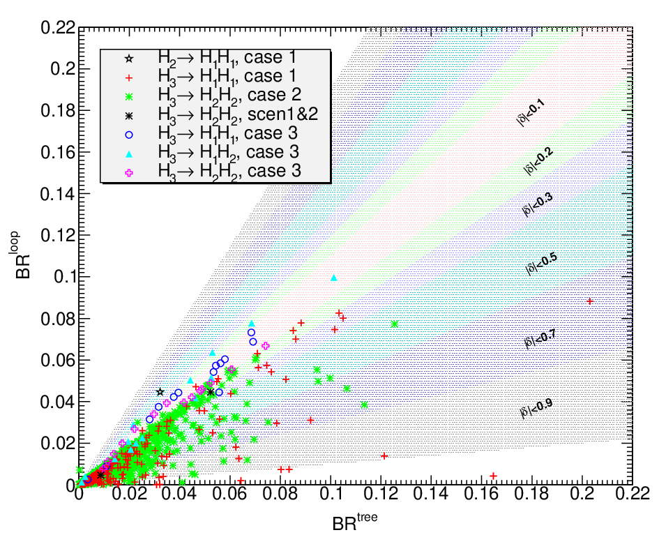
search for the heavy Higgs bosons, which can possibly be detected at the LHC via their decay into a pair of lighter Higgs bosons, which then subsequently decay further into SM particles. Figure 5 shows the branching ratios of the decay of a heavy CP-even Higgs boson, or depending on the scenario, into two SM-like Higgs bosons including loop-corrected trilinear Higgs self-couplings, as defined in Eq. (55), versus the branching ratio evaluated with tree-level trilinear couplings (cf. Eq. (55) without the 1-point irreducible contributions). The three different cases refer to scenarios with the SM-like Higgs boson being , (case 1), with being SM-like, (case 2), and with two light Higgs bosons and both having mass around 125 GeV and the combined Higgs rates being compatible with the SM rates (case 3). As can be inferred from the figure, which only includes scenarios compatible with our constraints, the loop-corrected trilinear Higgs coupling has the tendency to decrease the branching ratio compared to the tree-level result. The deviations can be as large as 90% in terms of the tree-level branching ratio, in some cases even higher. Also shown by black filled stars are two scenarios, where the SM-like Higgs boson is given by . The corresponding tree-level and loop corrected branching ratios amount to
These two scenarios scen1 and scen2 have the characteristic feature of
being excluded if loop corrections are not taken into account. In
scen1 the tree-level branching ratio of the SM-like decay into
is as large as 0.02. This decreases the branching ratios into the
other SM particles so that the scenario would be excluded because the
reduced signal strength in the final state drops below 0.8 and
the constraints Eq. (2.)) are not
fulfilled any more. Only the inclusion of the loop corrections decreases
the branching ratio into to so that the
scenario meets the constraints Eq. (2.)). In scen2 it is the branching ratio of
the decay which is as large as 0.26 at tree-level
compared to 0.1 after the inclusion of loop corrections, so that the
scenario is not valid at tree-level due to too small reduced signal strengths
in the and final states, unless loop
corrections are included. These examples demonstrate the importance of
including the
higher order corrections in order to properly interpret the NMSSM
spectrum with respect to the experimental findings.


In Fig. 6 left (right) we show the remaining possible branching
ratios of heavy scalar (pseudoscalar) Higgs bosons into a pair of
lighter Higgs bosons. In the left figure, the full black triangle corresponds to the
decay of scen1 and the black cross to the decay of
of scen2. The significant loop corrections leading to
deviations of up to 90%, respectively 70%, in terms of the
corresponding tree-level decay are crucial for the two scenarios to be
still in accordance with the LHC constraints Eq. (2.)). In
the right figure, the black squares are the branching ratio values of
the decay in scen1 and scen2, respectively. In this
decay the deviations between the tree-level and loop-corrected branching
ratios are small, less than 0.1 for both scenarios.
Figure 7 shows the branching ratio of the SM-like decay into as a function of (left) and of (right), evaluated at tree-level and at loop level. All the box points are allowed points, while the red star points do not fulfill our constraints. The figure shows that there are scenarios that would be excluded at tree-level, but are allowed once loop corrections are taken into account, which suppress the non-SM decays into Higgs boson pairs, so that the branching ratios into the SM particles remain compatible with the experimental constraints. The point of scen1 in Fig. 5 corresponds to in Fig. 7 (left) and to in Fig. 7 (right). The plots illustrate once more the importance of loop corrections when considering a specific model in light of the experimental results. As can be inferred from the figure, the loop corrections not only change the absolute value of the branching ratio but also shift the minimum to different values. The corresponding plots for a variation of the other parameters or show a similar behaviour.


4.4 Pair production of neutral Higgs bosons at the LHC
We apply the results of our calculation of the loop-corrected Higgs boson self-couplings to the pair production of neutral Higgs bosons at the LHC in order to study the effects of the higher order corrections. Higgs pair production processes are important as they give access to the trilinear Higgs self-couplings. The measurement of the trilinear and quartic Higgs self-interactions allows for the reconstruction of the Higgs potential which represents the ultimate check in the program of the experimental verification of the Higgs mechanism [5, 6]. The main contribution to Higgs pair production at the LHC comes from fusion [63, 64, 65]. Higgs pair production processes through vector boson fusion[66], double Higgs-strahlung [67] and associated production of a Higgs boson pair with [68] are less important [8] so that we focus here on the gluon fusion channel, namely the production of a pair of SM-like Higgs bosons in the framework of the NMSSM.
4.5 SM-like Higgs boson pair production through fusion
At leading order, the gluon fusion process into two SM-like Higgs bosons ( depending on the chosen parameter set),
| (93) |
consists of triangle, box and two-point contributions mediated by top and bottom (s)quarks, cf. Fig. 8.

The diagrams are similar to the MSSM case
[64, 65], except for the ones involving a
scalar Higgs boson in the -channel, which gets contributions from all
possible three neutral NMSSM Higgs bosons, that subsequently split
via the corresponding trilinear Higgs coupling into the final state
Higgs pair. Thus the production involves the trilinear Higgs
self-couplings and (). The NLO QCD
corrections have been calculated both for the SM and the MSSM case
in the limit of heavy loop particle masses. The corrections are
large, of [65], and therefore have
to be taken into account for a realistic assessment of the process.
We use the public Fortran code HPAIR [69] which computes
the QCD corrected
gluon fusion processes into pairs of Higgs bosons within the SM and
the MSSM, by applying the low-energy theorem. As claimed in [65],
this approximation is good for small values of in the MSSM
and for Higgs boson masses below .66
6
For further
discussion of the application of the low-energy theorem to single
and double Higgs production, see [70]. This is the
case for the here
considered pair production of a SM-like NMSSM Higgs boson, hence with
mass of about 125 GeV. Furthermore, in the NMSSM small
values are preferred in this case. We have modified the code HPAIR to include the additional contributions to the triangle
diagrams from the enlarged Higgs sector of the NMSSM and by replacing
the involved Higgs Yukawa and trilinear Higgs couplings with the
appropriate NMSSM Higgs couplings as discussed in subsection 4.2.
In the following, we present results for the pair production of two
SM-like Higgs bosons, . The scan performed in the
NMSSM parameter space resulted in numerous scenarios, where the
heavier scalar Higgs bosons can decay into
two on-shell Higgs bosons , leading to resonantly enhanced
contributions to the total pair production cross section. The program
HPAIR computes the resonantly enhanced diagrams together with the
remaining diagrams up to NLO QCD by making use of Breit-Wigner propagators
for the intermediate Higgs bosons. Alternatively, the non-resonant
contributions can be calculated by HPAIR at NLO QCD while the resonant ones
are obtained by multiplying the cross section of a singly produced
heavy Higgs boson with its branching ratio into . For comparison, we have also
calculated the cross section in this approach, which of
course neglects off-shell effects and interference terms between
non-resonant and resonant contributions. The cross
section for single Higgs production is obtained with the
Fortran code HIGLU [71] and is calculated at NLO
QCD to match the same order in as in Higgs pair
production.77
7
The program HIGLU includes the QCD
corrections to quark
loops up to NNLO QCD, taking into account the full mass dependence at
NLO QCD [72]. The NLO QCD corrections to the squark loops
have been implemented in the limit of heavy squark masses
[73], which is a good approximation for squark masses
above about 400 GeV. For the finite squark mass effects on
the NLO QCD corrections to Higgs production through gluon fusion, see
[74]. In HIGLU the Higgs Yukawa
couplings have been replaced by the corresponding couplings of the produced
NMSSM Higgs boson. The non-resonant and
resonant contributions are then summed up to get the total cross
section. We have compared the results obtained within the two approaches,
and the difference has been found to be less than 10% for our scenarios.
Note, that
the theoretical uncertainty on the NLO QCD double Higgs production
cross section due to unknown higher order corrections
[65] is larger than for single Higgs production at NLO
QCD [75]. All results presented hereafter have been
obtained with HPAIR. We emphasize that, if not stated otherwise,
in our calculation we have included the loop-corrected effective
trilinear Higgs couplings, presented in subsection
4.2, and the involved Higgs bosons both in the final
state and in the -channel exchange are the loop-corrected Higgs
states. All involved loop quantities are taken at zero external momentum.
The hadronic cross sections for SM-like Higgs boson pair production have been computed with MSTW 2008 NLO parton distribution functions (PDF) [76]. The factorization scale has been taken equal to the renormalisation scale and set equal to the invariant mass of the produced Higgs boson pair. In the code HPAIR top and bottom quark pole masses are used as default inputs.
4.6 Results for Higgs boson pair production
In Table 1 we show five sample scenarios compatible with the constraints according to Eq. (2.)), where is SM-like (points 1,2), is SM-like (points 4,5), and where and are close in mass with being near 125 GeV (point 3). In all scenarios the mass is large enough to allow for resonantly enhanced pair production from the
| Point 1 | 1.90 | 328 | 175 | 0.565 | 0.406 | -324 | 710 | 124 | 146 | 342 | 324 | 371 |
| Point 2 | 2.23 | 327 | 147 | 0.62 | 0.32 | -36.0 | 738 | 125.7 | 143 | 344 | 153 | 333 |
| Point 3 | 2.28 | 278 | 121 | 0.507 | 0.349 | -116 | 706 | 122 | 125.8 | 294 | 200 | 280 |
| Point 4 | 2.69 | 302 | 124 | 0.41 | 0.53 | -533 | 698 | 111 | 124.2 | 313 | 296 | 509 |
| Point 5 | 3.50 | 310 | 113 | 0.23 | 0.53 | -984 | 686 | 110 | 124.4 | 311 | 300 | 871 |
decay of , which can lead to a significant increase of the Higgs pair production cross section depending on the trilinear Higgs self-coupling . Table 2 contains the cross sections including NLO QCD corrections for the production of a pair of SM-like Higgs bosons in the five scenarios. Here denotes the cross sections calculated using the effective tree-level trilinear Higgs couplings , while the cross section values use the effective loop-corrected trilinear Higgs self-couplings . The Higgs boson masses are taken at loop level in both cases. The quantity is the difference between the two cross sections in terms of ,
| (94) |
The cross section values vary significantly in the various scenarios.
As can be inferred from the table, the differences in the cross
sections due to the inclusion of loop corrections in the trilinear
Higgs self-couplings can be substantial, ranging from nearly 40% to
almost 90% in terms of the tree-level cross section for the chosen scenarios.
| Point 1 | 485.9(4) | 55.08(4) | -0.89 |
|---|---|---|---|
| Point 2 | 462.9(3) | 254.2(2) | -0.45 |
| Point 3 | 374.3(3) | 175.5(1) | -0.53 |
| Point 4 | 99.30(7) | 28.36(2) | -0.71 |
| Point 5 | 17.52(1) | 24.05(2) | 0.37 |
In Fig. 9 (left) we show the gluon fusion production cross section of a pair of SM-like Higgs bosons calculated with the effective loop-corrected trilinear Higgs couplings, as a function of the ratio . Note that in the ratio refers to the trilinear Higgs self-coupling of the SM-like Higgs boson . In the case 3 of two Higgs bosons nearby 125 GeV, the name SM-like Higgs boson refers to the Higgs boson with the most SM-like Higgs Yukawa coupling to top quarks, as this coupling determines the dominant Higgs production cross section through gluon fusion and has the major impact on the Higgs production rate. The c.m. energy has been taken to be 14 TeV. Shown are cross sections for scenarios with (case 1), with (case2) or with two Higgs bosons with mass around 125 GeV building up the Higgs signal (case 3). The two black stars refer to scen1 and scen2 defined in section 4.3. Also plotted as a horizontal line is the SM cross section evaluated with . The cross section amounts to 35 fb compared to 34 fb evaluated with the tree-level coupling [8]. Furthermore, we plot as horizontal lines the results for the SM cross section in case of a variation of the effective loop-corrected trilinear coupling in terms of by a factor 2 and by a factor -1 and in case of . They show the sensitivity of the SM cross section to the trilinear Higgs self-coupling. In other words, they give an idea of how precisely the cross section has to be measured to achieve a certain accuracy in the trilinear SM Higgs self-coupling extracted from it. Many of the NMSSM cross section values lie nearby the SM result, independently of the ratio between the NMSSM and SM effective loop-corrected trilinear couplings, thus mimicking the SM case. However, there are also parameter points where the NMSSM and SM cross section differ significantly, so that a distinction of the two models would be possible. Loop corrections play here a crucial role:


In Fig. 9 (right) we show for the cases 1-3 the SM-like Higgs pair production cross section of the NMSSM evaluated with the effective loop-corrected trilinear Higgs self-couplings versus the cross section evaluated with the effective tree-level couplings. The difference between the cross sections is again quantified by , defined in Eq. (94). There are many scenarios with up to 50% and even higher. These large deviations can be traced back to the large deviations between the tree-level and loop-corrected branching ratios of the decay into two SM-like Higgs bosons , cf. Fig. 5.88 8 In the narrow-width approximation the Higgs pair production cross section is given by single Higgs production times the branching ratio BR(). The fact that, depending on whether or not the loop corrections to the trilinear Higgs self-couplings are included the scenario is distinguishable or not from the SM, clearly shows the importance of the loop corrections to obtain predictions useful for the experiments.
5 Conclusions
The discovery of a new scalar particle by the LHC experiments ATLAS
and CMS has triggered a lot of activities to determine the properties
of this particle. While the analyses of the so far accumulated data
strongly suggest that it is indeed the Higgs boson, i.e. the
particle responsible for the creation of particle masses without
violating gauge principles, the accumulation of more data is necessary for
its interpretation with respect to other models than the SM. The question has to
be clarified if it is the Higgs boson of the SM or of some extensions
beyond the SM. Among these, supersymmetric theories represent one of
the most intensely studied model classes. The Higgs sector of the NMSSM
consists of seven Higgs bosons entailing a rich phenomenology with
possible Higgs-to-Higgs decays and resonantly enhanced double Higgs
production cross sections due to heavier Higgs bosons decaying into a
pair of light Higgs particles.
In order to properly interpret the
experimental data and distinguish between different models the precise
prediction of the Higgs parameters such as masses and couplings,
including higher order corrections, is indispensable. The Higgs boson
masses and Higgs self-couplings are related to each other via the
Higgs potential. The prediction of loop-corrected Higgs boson masses
necessitates also the inclusion of loop corrections to the Higgs
self-couplings for a consistent analysis of the Higgs data. Having
calculated in previous works the one-loop corrected NMSSM Higgs boson
masses, in this contribution we extend our program of the calculation
of loop-corrected NMSSM Higgs parameters to the computation of
loop-corrected trilinear Higgs self-couplings.
The inclusion of loop corrections turns out to be important. We found
for example that non-SM Higgs decays of the
125 GeV NMSSM Higgs boson into a pair of lighter Higgs bosons
could be large enough to decrease the
signal strengths into SM particle final states so that they are not
compatible any more with the experimental results. The inclusion
of loop corrections to the trilinear couplings can, however, reduce
these rates to a level where the theoretical predictions are in
accordance with the experimental findings. In principle this could
also work the other way around, i.e. a scenario could be allowed
if the tree-level trilinear Higgs couplings are used, but excluded
in case of loop-corrected couplings. Trilinear Higgs self-couplings
of course also play a role in the decays of heavier non-SM-like Higgs
bosons into light Higgs pairs and their possible detection via these
decays.
Trilinear Higgs self-couplings enter the production of Higgs boson
pairs, so that they can be
extracted from the measurement of these processes. Once the (trilinear
and quartic) Higgs
self-couplings are known, the Higgs potential can be reconstructed to
perform the ultimate step in the experimental verification of the Higgs
mechanism. We found that the inclusion of loop corrections to the
trilinear Higgs self-couplings can alter the Higgs pair production
cross sections through gluon fusion substantially. In many of the
scenarios passing the constraints, the production
cross section of a pair of SM-like Higgs bosons with mass of 125 GeV
can be different enough to distinguish it from SM Higgs boson pair
production. This depends of course also on the experimental accuracy which
can be reached in these processes and which relies on analyses to be
performed at the high-energy and high-luminosity run of the LHC.
In summary, the computation of loop corrections to Higgs boson self-couplings and their inclusion in the analyses of the experimental results is crucial, in particular for the proper interpretation of the Higgs data with respect to the exclusion or non-exclusion of NMSSM parameter scenarios and/or with respect to the correct interpretation of Higgs pair production processes.
Acknowledgments
DTN, MMM and KW are supported by the DFG SFB/TR9 “Computational Particle Physics”. We thank Julien Baglio and Ramona Gröber for discussions. We would like to thank Pietro Slavich for the communication concerning the two-loop contribution to the NMSSM Higgs boson masses.
Appendix A Tree-level trilinear Higgs couplings
In this appendix we present the trilinear Higgs self-couplings of the interaction eigenstates of the NMSSM Higgs sector. The tree-level trilinear couplings of the scalar mass eigenstates () are obtained by applying the tree-level rotation matrices , Eq. (22), on the three interaction eigenstates,
| (95) |
The indices refer to the interaction eigenstates, and we have the following correspondences , , . The couplings are symmetric in the three indices. Using the short-hand notations , we have
| (96) | ||||||||
The trilinear couplings of one CP-even Higgs boson with two CP-odd Higgs states () are obtained from the interaction eigenstates through
| (97) |
Here, for the indices we have the correspondences , , . The couplings are symmetric with respect to an exchange of the last two indices , and
| (98) |
References
- [1] G. Aad et al. [ATLAS Collaboration], Phys. Lett. B 716 (2012) 1 [arXiv:1207.7214 [hep-ex]]; G. Aad et al. [ATLAS Collaboration], ATLAS-CONF-2012-162.
- [2] S. Chatrchyan et al. [CMS Collaboration], Phys. Lett. B 716 (2012) 30 [arXiv:1207.7235 [hep-ex]]; S. Chatrchyan et al. [CMS Collaboration], CMS-PAS-HIG-12-045.
- [3] C. Englert, T. Plehn, M. Rauch, D. Zerwas and P. M. Zerwas, Phys. Lett. B 707 (2012) 512 [arXiv:1112.3007 [hep-ph]]; J. R. Espinosa, C. Grojean, M. Muhlleitner and M. Trott, JHEP 1205 (2012) 097 [arXiv:1202.3697 [hep-ph]]; P. P. Giardino, K. Kannike, M. Raidal and A. Strumia, JHEP 1206 (2012) 117 [arXiv:1203.4254 [hep-ph]]; J. Ellis and T. You, JHEP 1206 (2012) 140 [arXiv:1204.0464 [hep-ph]]; A. Azatov, R. Contino, D. Del Re, J. Galloway, M. Grassi and S. Rahatlou, JHEP 1206 (2012) 134 [arXiv:1204.4817 [hep-ph]]. M. Klute, R. Lafaye, T. Plehn, M. Rauch and D. Zerwas, Phys. Rev. Lett. 109 (2012) 101801 [arXiv:1205.2699 [hep-ph]]; I. Low, J. Lykken and G. Shaughnessy, Phys. Rev. D 86 (2012) 093012 [arXiv:1207.1093 [hep-ph]]; T. Corbett, O. J. P. Eboli, J. Gonzalez-Fraile and M. C. Gonzalez-Garcia, Phys. Rev. D 86 (2012) 075013 [arXiv:1207.1344 [hep-ph]]; P. P. Giardino, K. Kannike, M. Raidal and A. Strumia, Phys. Lett. B 718 (2012) 469 [arXiv:1207.1347 [hep-ph]]; J. Ellis and T. You, JHEP 1209 (2012) 123 [arXiv:1207.1693 [hep-ph]]; J. R. Espinosa, C. Grojean, M. Muhlleitner and M. Trott, JHEP 1212 (2012) 045 [arXiv:1207.1717 [hep-ph]]; D. Carmi, A. Falkowski, E. Kuflik, T. Volansky and J. Zupan, JHEP 1210 (2012) 196 [arXiv:1207.1718 [hep-ph]]; F. Bonnet, T. Ota, M. Rauch and W. Winter, Phys. Rev. D 86 (2012) 093014 [arXiv:1207.4599 [hep-ph]]; T. Plehn and M. Rauch, Europhys. Lett. 100 (2012) 11002 [arXiv:1207.6108 [hep-ph]]; G. Moreau, Phys. Rev. D 87 (2013) 015027 [arXiv:1210.3977 [hep-ph]].
- [4] See e.g.: D. J. Miller, 2, S. Y. Choi, B. Eberle, M. M. Muhlleitner and P. M. Zerwas, Phys. Lett. B 505 (2001) 149 [hep-ph/0102023]; T. Plehn, D. L. Rainwater and D. Zeppenfeld, Phys. Rev. Lett. 88 (2002) 051801 [hep-ph/0105325]; S. Y. Choi, D. J. Miller, M. M. Muhlleitner and P. M. Zerwas, Phys. Lett. B 553 (2003) 61 [hep-ph/0210077]; K. Odagiri, JHEP 0303 (2003) 009 [hep-ph/0212215]; C. P. Buszello, I. Fleck, P. Marquard and J. J. van der Bij, Eur. Phys. J. C 32 (2004) 209 [hep-ph/0212396]; J. R. Ellis, J. S. Lee and A. Pilaftsis, Phys. Rev. D 70 (2004) 075010 [hep-ph/0404167]; S. Y. Choi, J. Kalinowski, Y. Liao and P. M. Zerwas, Eur. Phys. J. C 40 (2005) 555 [hep-ph/0407347]. C. P. Buszello and P. Marquard, hep-ph/0603209; R. M. Godbole, D. J. Miller and M. M. Muhlleitner, JHEP 0712 (2007) 031 [arXiv:0708.0458 [hep-ph]]; S. Berge, W. Bernreuther and J. Ziethe, Phys. Rev. Lett. 100 (2008) 171605 [arXiv:0801.2297 [hep-ph]]; S. Berge and W. Bernreuther, Phys. Lett. B 671 (2009) 470 [arXiv:0812.1910 [hep-ph]]; K. Hagiwara, Q. Li and K. Mawatari, JHEP 0907 (2009) 101 [arXiv:0905.4314 [hep-ph]]; Y. Gao, A. V. Gritsan, Z. Guo, K. Melnikov, M. Schulze and N. V. Tran, Phys. Rev. D 81 (2010) 075022 [arXiv:1001.3396 [hep-ph]]; A. De Rujula, J. Lykken, M. Pierini, C. Rogan and M. Spiropulu, Phys. Rev. D 82 (2010) 013003 [arXiv:1001.5300 [hep-ph]]; N. D. Christensen, T. Han and Y. Li, Phys. Lett. B 693 (2010) 28 [arXiv:1005.5393 [hep-ph]]; C. Englert, C. Hackstein and M. Spannowsky, Phys. Rev. D 82 (2010) 114024 [arXiv:1010.0676 [hep-ph]]; U. De Sanctis, M. Fabbrichesi and A. Tonero, Phys. Rev. D 84 (2011) 015013 [arXiv:1103.1973 [hep-ph]]; S. Berge, W. Bernreuther, B. Niepelt and H. Spiesberger, Phys. Rev. D 84 (2011) 116003 [arXiv:1108.0670 [hep-ph]]. J. Ellis and D. S. Hwang, JHEP 1209 (2012) 071 [arXiv:1202.6660 [hep-ph]]; C. Englert, M. Spannowsky and M. Takeuchi, JHEP 1206 (2012) 108 [arXiv:1203.5788 [hep-ph]]; S. Bolognesi, Y. Gao, A. V. Gritsan, K. Melnikov, M. Schulze, N. V. Tran and A. Whitbeck, Phys. Rev. D 86 (2012) 095031 [arXiv:1208.4018 [hep-ph]]; R. Boughezal, T. J. LeCompte and F. Petriello, arXiv:1208.4311 [hep-ph]; D. Stolarski and R. Vega-Morales, Phys. Rev. D 86 (2012) 117504 [arXiv:1208.4840 [hep-ph]]; J. Ellis, D. S. Hwang, V. Sanz and T. You, JHEP 1211 (2012) 134 [arXiv:1208.6002 [hep-ph]]; A. Alves, Phys. Rev. D 86 (2012) 113010 [arXiv:1209.1037 [hep-ph]]. S. Y. Choi, M. M. Muhlleitner and P. M. Zerwas, Phys. Lett. B 718 (2013) 1031 [arXiv:1209.5268 [hep-ph]]; J. Ellis, R. Fok, D. S. Hwang, V. Sanz and T. You, arXiv:1210.5229 [hep-ph]; J. Ellis, R. Fok, D. S. Hwang, V. Sanz and T. You, arXiv:1210.5229 [hep-ph]; Y. Chen, N. Tran and R. Vega-Morales, JHEP 1301 (2013) 182 [arXiv:1211.1959 [hep-ph]]; A. Freitas and P. Schwaller, Phys. Rev. D 87 (2013) 055014 [arXiv:1211.1980 [hep-ph]]; J. Frank, M. Rauch and D. Zeppenfeld, Phys. Rev. D 87, 055020 (2013) [arXiv:1211.3658 [hep-ph]]; C. Englert, D. Goncalves-Netto, K. Mawatari and T. Plehn, JHEP 1301 (2013) 148 [arXiv:1212.0843 [hep-ph]]; A. Djouadi, R. M. Godbole, B. Mellado and K. Mohan, arXiv:1301.4965 [hep-ph]; J. Frank, M. Rauch and D. Zeppenfeld, arXiv:1305.1883 [hep-ph]; R. Godbole, D. J. Miller, K. Mohan and C. D. White, arXiv:1306.2573 [hep-ph].
- [5] A. Djouadi, W. Kilian, M. Muhlleitner and P. M. Zerwas, Eur. Phys. J. C 10 (1999) 27 [hep-ph/9903229].
- [6] A. Djouadi, W. Kilian, M. Muhlleitner and P. M. Zerwas, Eur. Phys. J. C 10 (1999) 45 [hep-ph/9904287]; M. M. Muhlleitner, hep-ph/0008127.
- [7] U. Baur, T. Plehn and D. L. Rainwater, Phys. Rev. Lett. 89 (2002) 151801; Phys. Rev. D 67 (2003) 033003; Phys. Rev. D 68 (2003) 033001; Phys. Rev. D 69 (2004) 053004; R. Grober and M. Muhlleitner, JHEP 1106 (2011) 020 [arXiv:1012.1562 [hep-ph]]; M. J. Dolan, C. Englert and M. Spannowsky, JHEP 1210 (2012) 112 [arXiv:1206.5001 [hep-ph]]; A. Papaefstathiou, L. L. Yang and J. Zurita, Phys. Rev. D 87 (2013) 011301 [arXiv:1209.1489 [hep-ph]]; F. Goertz, A. Papaefstathiou, L. L. Yang and J. Zurita, arXiv:1301.3492 [hep-ph]; J. Grigo, J. Hoff, K. Melnikov and M. Steinhauser, arXiv:1305.7340 [hep-ph].
- [8] J. Baglio, A. Djouadi, R. Grober, M. M. Muhlleitner, J. Quevillon and M. Spira, arXiv:1212.5581 [hep-ph].
- [9] G. Cynolter, E. Lendvai and G. Pocsik, Acta Phys. Polon. B 31 (2000) 1749 [hep-ph/0003008]; T. Plehn and M. Rauch, Phys. Rev. D 72 (2005) 053008 [hep-ph/0507321]; T. Binoth, S. Karg, N. Kauer and R. Ruckl, Phys. Rev. D 74 (2006) 113008 [hep-ph/0608057].
- [10] See e.g. with references therein: A. Djouadi, Phys. Rept. 459 (2008) 1 [hep-ph/0503173].
- [11] P. Fayet, Nucl. Phys. B 90 (1975) 104; Phys. Lett. B 64 (1976) 159; Phys. Lett. B 69 (1977) 489 and Phys. Lett. B 84 (1979) 416; H.P. Nilles, M. Srednicki and D. Wyler, Phys. Lett. B 120 (1983) 346; J.M. Frere, D.R. Jones and S. Raby, Nucl. Phys. B 222 (1983) 11; J.P. Derendinger and C.A. Savoy, Nucl. Phys. B 237 (1984) 307; A.I. Veselov, M.I. Vysotsky and K.A. Ter-Martirosian, Sov. Phys. JETP 63 (1986) 489; J.R. Ellis, J.F. Gunion, H.E. Haber, L. Roszkowski and F. Zwirner, Phys. Rev. D 39 (1989) 844; M. Drees, Int. J. Mod. Phys. A 4 (1989) 3635.
- [12] U. Ellwanger, M. Rausch de Traubenberg and C.A. Savoy, Phys. Lett. B 315 (1993) 331, Z. Phys. C 67 (1995) 665 and Nucl. Phys. B 492 (1997) 307; U. Ellwanger, Phys. Lett. B 303 (1993) 271; P. Pandita, Z. Phys. C 59 (1993) 575; T. Elliott, S.F. King and P.L. White, Phys. Rev. D 49 (1994) 2435; S.F. King and P.L. White, Phys. Rev. D 52 (1995) 4183; F. Franke and H. Fraas, Int. J. Mod. Phys. A 12 (1997) 479.
- [13] D. J. Miller, R. Nevzorov and P. M. Zerwas, Nucl. Phys. B 681 (2004) 3 [hep-ph/0304049]; for reviews, see: M. Maniatis, Int. J. Mod. Phys. A25 (2010) 3505 [arXiv:0906.0777 [hep-ph]]; U. Ellwanger, C. Hugonie, A. M. Teixeira, Phys. Rept. 496 (2010) 1 [arXiv:0910.1785 [hep-ph]]; U. Ellwanger, Eur. Phys. J. C 71 (2011) 1782 [arXiv:1108.0157 [hep-ph]].
- [14] K. Ender, T. Graf, M. Muhlleitner and H. Rzehak, Phys. Rev. D 85 (2012) 075024 [arXiv:1111.4952 [hep-ph]].
- [15] T. Graf, R. Grober, M. Muhlleitner, H. Rzehak and K. Walz, JHEP 1210 (2012) 122 [arXiv:1206.6806 [hep-ph]].
- [16] J.E. Kim and H.P. Nilles, Phys. Lett. B 138 (1984) 150.
- [17] M. Bastero-Gil, C. Hugonie, S. F. King, D. P. Roy and S. Vempati, Phys. Lett. B 489, 359 (2000) [hep-ph/0006198]; A. Delgado, C. Kolda, J. P. Olson and A. de la Puente, Phys. Rev. Lett. 105, 091802 (2010) [arXiv:1005.1282 [hep-ph]]; U. Ellwanger, G. Espitalier-Noel and C. Hugonie, JHEP 1109 (2011) 105 [arXiv:1107.2472 [hep-ph]]; G. G. Ross and K. Schmidt-Hoberg, arXiv:1108.1284 [hep-ph].
- [18] U. Ellwanger, Phys. Lett. B303 (1993) 271 [hep-ph/9302224]; T. Elliott, S. F. King, P. L. White, Phys. Lett. B305 (1993) 71 [hep-ph/9302202], Phys. Lett. B314 (1993) 56 [hep-ph/9305282], Phys. Rev. D49 (1994) 2435 [hep-ph/9308309]; P. N. Pandita, Z. Phys. C59 (1993) 575, Phys. Lett. B318 (1993) 338.
- [19] U. Ellwanger, C. Hugonie, Phys. Lett. B623 (2005) 93 [hep-ph/0504269].
- [20] G. Degrassi and P. Slavich, Nucl. Phys. B 825 (2010) 119 [arXiv:0907.4682 [hep-ph]].
- [21] F. Staub, W. Porod, B. Herrmann, JHEP 1010 (2010) 040 [arXiv:1007.4049 [hep-ph]].
- [22] S. W. Ham, J. Kim, S. K. Oh and D. Son, Phys. Rev. D 64 (2001) 035007 [hep-ph/0104144]; S. W. Ham, S. H. Kim, S. K. OH and D. Son, Phys. Rev. D 76 (2007) 115013 [arXiv:0708.2755 [hep-ph]].
- [23] S. W. Ham, S. K. Oh and D. Son, Phys. Rev. D 65 (2002) 075004 [hep-ph/0110052]; S. W. Ham, Y. S. Jeong and S. K. Oh, hep-ph/0308264.
- [24] K. Funakubo and S. Tao, Prog. Theor. Phys. 113 (2005) 821 [hep-ph/0409294].
- [25] K. Cheung, T. -J. Hou, J. S. Lee and E. Senaha, Phys. Rev. D 82 (2010) 075007 [arXiv:1006.1458 [hep-ph]].
- [26] A. Denner, Fortsch. Phys. 41 (1993) 307 [arXiv:0709.1075 [hep-ph]].
- [27] K. Melnikov and T. v. Ritbergen, Phys. Lett. B 482 (2000) 99 [hep-ph/9912391].
- [28] M. S. Carena, D. Garcia, U. Nierste and C. E. M. Wagner, Nucl. Phys. B 577 (2000) 88 [hep-ph/9912516].
- [29] L. V. Avdeev and M. Y. Kalmykov, Nucl. Phys. B 502 (1997) 419 [hep-ph/9701308].
- [30] D. M. Pierce, J. A. Bagger, K. T. Matchev and R. -j. Zhang, Nucl. Phys. B 491 (1997) 3 [hep-ph/9606211].
- [31] M. S. Carena, J. R. Ellis, S. Mrenna, A. Pilaftsis and C. E. M. Wagner, Nucl. Phys. B 659 (2003) 145 [hep-ph/0211467].
- [32] J. Guasch, P. Hafliger and M. Spira, Phys. Rev. D 68 (2003) 115001 [hep-ph/0305101]; D. Noth and M. Spira, Phys. Rev. Lett. 101 (2008) 181801 [arXiv:0808.0087 [hep-ph]]; D. Noth and M. Spira, JHEP 1106 (2011) 084 [arXiv:1001.1935 [hep-ph]]; L. Mihaila and C. Reisser, JHEP 1008 (2010) 021 [arXiv:1007.0693 [hep-ph]].
- [33] A. Dabelstein, Nucl. Phys. B 456 (1995) 25 [hep-ph/9503443].
- [34] M. Frank, T. Hahn, S. Heinemeyer, W. Hollik, H. Rzehak, and G. Weiglein, JHEP 0702 (2007) 047 [hep-ph/0611326].
- [35] K. E. Williams and G. Weiglein, Phys. Lett. B 660 (2008) 217 [arXiv:0710.5320 [hep-ph]].
- [36] N. Baro, F. Boudjema and A. Semenov, Phys. Rev. D 78 (2008) 115003 [arXiv:0807.4668 [hep-ph]].
- [37] K. E. Williams, H. Rzehak and G. Weiglein, Eur. Phys. J. C 71 (2011) 1669 [arXiv:1103.1335 [hep-ph]].
- [38] F. Staub, [arXiv:0806.0538 [hep-ph]], Comput. Phys. Commun. 181 (2010) 1077 [arXiv:0909.2863 [hep-ph]], Comput. Phys. Commun. 182 (2011) 808 [arXiv:1002.0840 [hep-ph]].
- [39] J. Kublbeck, M. Bohm and A. Denner, Comput. Phys. Commun. 60 (1990) 165; T. Hahn, Comput. Phys. Commun. 140 (2001) 418 [hep-ph/0012260].
- [40] T. Hahn and M. Perez-Victoria, Comput. Phys. Commun. 118 (1999) 153 [hep-ph/9807565]; T. Hahn, Comput. Phys. Commun. 178 (2008) 217 [hep-ph/0611273].
- [41] J. Beringer et al. [Particle Data Group Collaboration], Phys. Rev. D 86 (2012) 010001.
- [42] F. Jegerlehner, Nuovo Cim. C 034S1 (2011) 31 [arXiv:1107.4683 [hep-ph]].
- [43] The ATLAS Collaboration, ATLAS-CONF-2013-047 and ATLAS-CONF-2012-104; The CMS Collaboration, arXiv:1212.6961 [hep-ex] and arXiv:1303.2985 [hep-ex].
- [44] The ATLAS Collaboration, ATLAS-CONF-2013-024; ATLAS-CONF-2013-025, ATLAS-CONF-2013-037; ATLAS-CONF-2013-048, ATLAS-CONF-2013-053; Eur. Phys. J. C 72 (2012) 2237 [arXiv:1208.4305 [hep-ex]]; Phys. Lett. B 720 (2013) 13 [arXiv:1209.2102 [hep-ex]]; The CMS Collaboration, CMS-PAS-SUS-13-011; arXiv:1212.6961 [hep-ex]; JHEP 1301 (2013) 077; CMS-PAS-SUS-11-030.
- [45] S. F. King, M. Muhlleitner and R. Nevzorov, Nucl. Phys. B 860 (2012) 207 [arXiv:1201.2671 [hep-ph]].
- [46] S. F. King, M. Muhlleitner, R. Nevzorov and K. Walz, Nucl. Phys. B 870 (2013) 323 [arXiv:1211.5074 [hep-ph]].
- [47] The ATLAS Collaboration, JHEP 1206 (2012) 039 [arXiv:1204.2760 [hep-ex]]; ATLAS-CONF-2012-011 and ATLAS-CONF-2011-094; The CMS Collaboration, JHEP 1207 (2012) 143 [arXiv:1205.5736 [hep-ex]].
- [48] The ATLAS Collaboration, ATLAS-CONF-2013-034.
- [49] The CMS Collaboration, CMS-PAS-HIG-13-005.
- [50] A. Djouadi, J. Kalinowski and M. Spira, Comput. Phys. Commun. 108, 56 (1998) [hep-ph/9704448].
- [51] A. Djouadi, M. M. Muhlleitner and M. Spira, Acta Phys. Polon. B 38 (2007) 635 [hep-ph/0609292].
- [52] U. Ellwanger, J.F. Gunion and C. Hugonie, JHEP 0502 (2005) 066; U. Ellwanger and C. Hugonie, Comput. Phys. Commun. 175 (2006) 290.
- [53]
U. Ellwanger and C. Hugonie, Comput. Phys. Commun. 177 (2007)
399;
(see also http://www.th.u-psud.fr/NMHDECAY/nmssmtools.html). - [54] M. Muhlleitner, A. Djouadi and Y. Mambrini, Comput. Phys. Commun. 168 (2005) 46 [hep-ph/0311167]; M. Muhlleitner, Acta Phys. Polon. B 35 (2004) 2753 [hep-ph/0409200].
- [55] P. Bechtle, O. Brein, S. Heinemeyer, G. Weiglein and K. E. Williams, Comput. Phys. Commun. 181 (2010) 138 [arXiv:0811.4169 [hep-ph]]; P. Bechtle, O. Brein, S. Heinemeyer, G. Weiglein and K. E. Williams, Comput. Phys. Commun. 182 (2011) 2605 [arXiv:1102.1898 [hep-ph]]; see also references therein.
- [56] The ATLAS Collaboration, ATLAS-CONF-2013-012 and ATLAS-CONF-2012-168; The CMS Collaboration, CMS-PAS-HIG-13-001.
- [57] The ATLAS Collaboration, ATLAS-CONF-2013-013; The CMS Collaboration, CMS-PAS-HIG-13-002.
- [58] The ATLAS Collaboration, ATLAS-CONF-2013-030.
- [59] S. Kanemura, Y. Okada, E. Senaha and C. -P. Yuan, Phys. Rev. D 70 (2004) 115002 [hep-ph/0408364].
- [60] W. Hollik and S. Penaranda, Eur. Phys. J. C 23 (2002) 163 [hep-ph/0108245].
- [61] A. Dobado, M. J. Herrero, W. Hollik and S. Penaranda, Phys. Rev. D 66 (2002) 095016 [hep-ph/0208014].
- [62] S. Kanemura, T. Shindou and K. Yagyu, Phys. Lett. B 699 (2011) 258 [arXiv:1009.1836 [hep-ph]].
- [63] E. W. N. Glover and J. J. van der Bij, Nucl. Phys. B 309 (1988) 282.
- [64] T. Plehn, M. Spira and P. M. Zerwas, Nucl. Phys. B 479 (1996) 46 [Erratum-ibid. B 531 (1998) 655] [hep-ph/9603205].
- [65] S. Dawson, S. Dittmaier and M. Spira, Phys. Rev. D 58 (1998) 115012 [hep-ph/9805244].
- [66] W. Y. Keung, Mod. Phys. Lett. A2 (1987) 765; D. Dicus, K. Kallianpur and S. Willenbrock, Phys. Lett. B200 (1988) 187; K. Kallianpur, Phys. Lett. B215 (1988) 392; A. Abbasabadi, W.W. Repko, D.A. Dicus and R. Vega, Phys. Rev. D38 (1988) 2770; Phys. Lett. B213 (1988) 386; A. Dobrovolskaya and V. Novikov, Z. Phys. C52 (1991) 427.
- [67] V. Barger, T. Han and R.J.N. Phillips, Phys. Rev. D38 (1988) 2766.
- [68] M. Moretti, S. Moretti, F. Piccinini, R. Pittau and A. D. Polosa, JHEP 0502 (2005) 024 [hep-ph/0410334].
- [69] URL: http://people.web.psi.ch/spira/hpair/
- [70] M. Gillioz, R. Grober, C. Grojean, M. Muhlleitner and E. Salvioni, JHEP 1210 (2012) 004 [arXiv:1206.7120 [hep-ph]].
- [71] M. Spira, hep-ph/9510347.
- [72] D. Graudenz, M. Spira and P. M. Zerwas, Phys. Rev. Lett. 70 (1993) 1372; M. Spira, A. Djouadi, D. Graudenz and P. M. Zerwas, Phys. Lett. B 318 (1993) 347; M. Spira, A. Djouadi, D. Graudenz and P. M. Zerwas, Nucl. Phys. B 453 (1995) 17 [hep-ph/9504378].
- [73] S. Dawson, A. Djouadi and M. Spira, Phys. Rev. Lett. 77 (1996) 16 [hep-ph/9603423].
- [74] M. Muhlleitner and M. Spira, Nucl. Phys. B 790 (2008) 1 [hep-ph/0612254].
- [75] S. Dittmaier et al. [LHC Higgs Cross Section Working Group Collaboration], arXiv:1101.0593 [hep-ph].
- [76] A. D. Martin, W. J. Stirling, R. S. Thorne and G. Watt, Eur. Phys. J. C 63 (2009) 189 [arXiv:0901.0002 [hep-ph]].