Polarization of photons scattered by electrons in any spectral distribution
Abstract
Based on the quantum electrodynamics, we present a generic formalism of the polarization for beamed monochromatic photons scattered by electrons in any spectral distribution. The formulae reduce to the components of the Fano matrix when electrons are at rest. We mainly investigate the polarization in three scenarios, i.e., electrons at rest, isotropic electrons with a power law spectrum and thermal electrons. If the incident beam is polarized, the polarization is reduced significantly by isotropic electrons at large viewing angles, and the degree of polarization due to thermal electrons is about one times less than that of electrons in a power law. If the incident bean is unpolarized, soft -rays can lead to about polarization at viewing angles around . For isotropic electrons, one remarkable feature is that the polarization as a function of the incident photon energy always peaks roughly at MeV, this is valid for both the thermal and power law cases. This feature can be used to distinguish the model of the inverse Compton scattering from that of the synchrotron radiation.
Keywords:
polarization - radiation mechanism: non-thermal - scatteringI Introduction
Synchrotron radiation (SR) and inverse Compton scattering (ICS) are considered most frequently as the main mechanisms of producing the X-ray and -ray in astrophysical objects such as the gamma-ray burst (GRB), the active galactic nuclei (AGN) and blazars. Besides light curves and spectra, the polarization is another important tool for the diagnosis of the emission mechanisms of the astrophysical objects, since the degree of polarization, orientation, and time variation can provide more information for analysis. Many models have been suggested to investigate the polarization of SR and ICS in different setups. The polarization of SR with power law distributed electrons in a uniform magnetic field is well-known, i.e., , where is the spectral index of electrons [32, 19, 20]. The investigation of ICS induced polarization is still in progress.
Bonometto et al., [9] presented a general formalism of the polarization in ICS for arbitrary distributions of photons and electrons in the Thomson limit. Later on, [10] used the same scenario to investigate the polarization for ICS with the SR source, they found that the initial polarization is preserved with a large fraction after ICS. Befelman & Sikora, [4] investigated the polarization in a system that the ambient isotropic radiation is scattered by the flow of cold electrons. Different geometrical structures of the electron jet (e.g., pencil beam or hollow cone) produce polarizations with different orientations. The initial ambient radiation is unpolarized, but the maximal polarization can be achieved at the viewing angle , where is the Lorentz factor of electrons. Celotti & Matt, [11] used the similar method to study the polarization properties of synchrotron self-Compton (SSC) emission for an isotropic electron distribution, their results roughly agree with that of Bonometto & Saggion, [10].
Aharonian & Atoyan, [3] considered the spectrum and polarization due to ICS. The formula of the polarization was given for the unpolarized initial beam. Numerical simulation for the isotropic electron distribution shows that a moderate linear polarization is still possible at large viewing angles [14]. McNamara et al., [25] investigated the polarization properties of X-rays in the AGN. Their simulations show that the polarization increases with the viewing angle for source photons emitted from an accretion disc or from the cosmic microwave background (CMB), and the maximal polarization is about . For the SSC case, they found that the resulting X-ray polarization depends strongly on the injection site of the seed photon, i.e., with typical for the emission near the jet base, while for the uniform emission throughout the jet.
GeV photons are observed in the prompt phase in some GRBs [1, 2]. Although the photon energy is much reduced in the jet frame by excluding the Lorentz effect, MeV photons are still popular in the jet frame in GRBs. If these photons are the results of ICS, the formalism of the polarization should be extended to the KN regime. Another shortcoming of these investigations is that the incident photons are unpolarized except SSC. Krawczynski, [23] used the Monte Carlo simulation to calculate the polarization of ICS in the KN regime for isotropic electrons, and found that the net polarization is zero, that is against the results given by McNamara et al., [25]. We presented a formalism of the polarization induced by cold electrons [13]. We found that the orientation of the polarization changes when the incident photons are of the SR origin, and the polarization reduces significantly in the KN regime. However, an analytical formalism of the polarization in the ICS process with arbitrary initial polarizations and electron spectra is still lacking.
In the present paper, we present an analytical formalism for the polarization induced by isotropic electrons with an arbitrary spectrum. First we consider the kinematics of the scattering of a photon by an electron. The cross section for the scattering of polarized photons by an unpolarized electron is used to obtain the Stokes parameters for the outgoing photon. In the framework of the quantum electrodynamics, we investigate the polarization effects induced by the isotropic electrons for both the polarized and unpolarized incident photons.When electrons are at rest, the components of the cross section reduce to the components of the Fano matrix. By numerical calculations, we discuss the polarization for electrons with power law and thermal distributions, respectively. The rest of the paper is arranged as follows. In Section II, we introduce the kinematics of the scattering, and present the formulae of the Stokes parameters for the scattered photon. In Section III, we investigate the polarization for three scenarios. Discussion and conclusions are given in Section IV.
II Polarization formula
The scattering process is illustrated in Fig. 1. The beam of photons produced by the synchrotron radiation of electrons is collimated roughly along the radial direction of the outflow, namely, the -direction. Suppose that a photon is injected along (we take the convention that a variable with a hat denotes the unit vector along that direction), it is scattered by an electron at point . Then, it goes toward the observer along the direction. The -axis is chosen in the and plane, and the axes form a right-handed set. The injected electron has an arbitrary momentum , where is the Lorentz factor of the electron, , and denotes the incident direction of the electron. The momentum of the injected electron can be described by spherical coordinates , and completely. is the polar angle between and , and is the azimuthal angle of relative to the -axis, measured counter clockwise from the observer side.
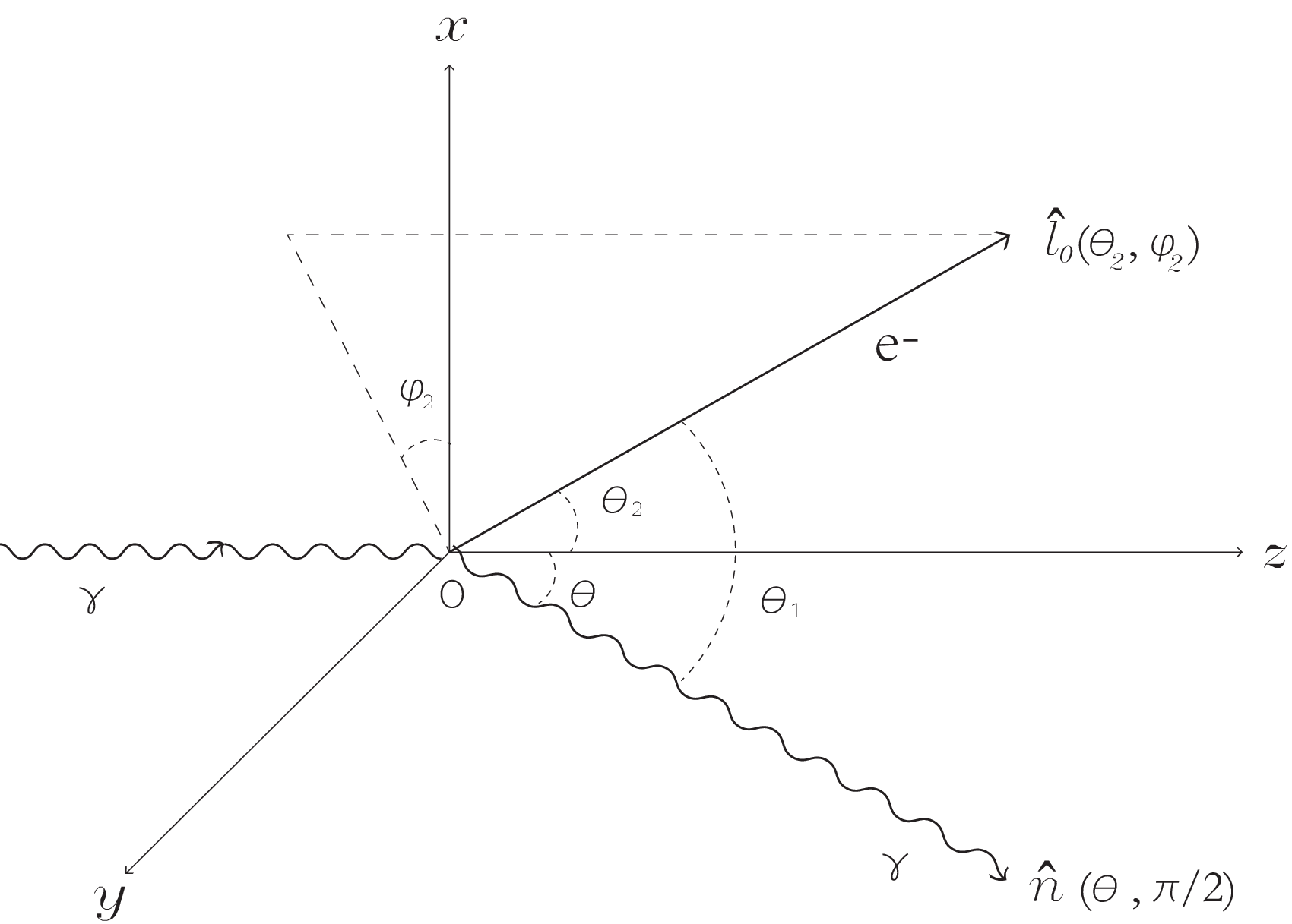
The four momenta of the electron before and after scattering process are written as and , respectively. In a similar way, the four momenta of the photon before and after scattering are written as and . The conservation of the energy and momentum of the system states that
| (1) |
After scattering, the photon energy is written as
| (2) |
The angle between and is denoted by , and the angle between and is denoted by . The geometrical relation gives
| (3) |
One can also calculate the Lorentz factor of the electron after scattering. However, they are not observable quantities and have no effects on the final polarization.
In quantum electrodynamics, a convenient way to describe the partial polarization is by using the density matrix in terms of three real Stokes parameters (). The density matrix is written as [6]
where the Stokes parameters are defined with respect to the axes . The positive (negative) describes that the photon is linearly polarized along the () axis, the parameter means the linear polarization along the directions with azimuthal angles relative to the axis in the plane, and the parameter describes the left-hand or the right-hand circular polarization. In terms of Stokes parameters , the polarization degree is written as
| (7) |
The Stokes parameters satisfy the condition . For , the photon is in a unpolarized state; for , the photon is completely polarized. In the case, we call that the photon is partially polarized.
When the and axes are rotated by an angle about the axis, one obtains a new coordinate frame. Respect to these new axes, the Stokes parameters transform as
| (8) |
Therefore, the circular polarization is unaffected by the rotation, while the values of and depend on the chosen of the axes. However, one can easily verify that the degree of the polarization is invariant under such rotation [24]. Another alternative manner to describe the polarization is by using four Stokes parameters , , , and [29], where is the total energy density of the photon. The three Stokes parameters correspond to , and normalized by , i.e., , and , respectively.
The differential cross section for the scattering of a polarized photon by an unpolarized electron is written as [6]
| (9) |
where
| (10) |
and is the classical electron radius. The Stokes parameters and () describe the polarizations of the incident and scattered photons, respectively. The parameters and are defined as
| (11) |
The dimensionless variables and originate from the Mandelstam variables, and are always positive according to this expression.
In the setup, we suppose that the injected electrons are isotropic in the jet frame. If the initial momenta and are given, the momentum of the scattered photon is a function of . Therefore, the differential of is written as
| (12) |
Taking use of Equations (2), (3), (9), (11) and (12), we rewrite the differential cross section as
| (13) |
where , and
| (14) |
The Stokes parameters of the secondary photon are denoted by , which are equal to the ratios of the coefficients of to the terms independent of in Equation (13) [6], i.e.,
| (15) |
Noticing that the circular polarization of the scattered photon occurs only if the incident photon is circularly polarized. The degree of polarization of the scattered photon can be expressed as
| (16) |
We consider that the incident photon beam is of the SR origin. Suppose that there is a uniform and static magnetic field in the plasma, the azimuthal angle of projected on the plane is denoted by . The definition of the polarization is , where and are the intensities along the direction and with the azimuthal angle and , respectively. The primary degree of the polarization of SR photons is . The Stokes parameters of the incident photons can be written as
| (17) |
When (the magnetic field is perpendicular to the scattering plane), one has and . The orientation of the polarization is along the axis. When , one has and . The orientation of the polarization is along the line rotating counter clockwise from the axis. Therefore, represents the initial polarization orientation. After being scattered by electrons, the direction of the polarization changes. are defined in a new coordinate axes, i.e., the axis is fixed and axis is rotated to coincide with the direction . Then, still describes the polarization along the axis, and describes the polarization along the line with azimuthal angle in the new set of axes.
III Effects of different electron spectra
The obtained final polarization is quite general. It depends on the spectra of incident photons and injected electrons. We investigate the polarization in three scenarios: electrons at rest, isotropic electrons with a power law distribution and electrons with the Maxwell distribution. For electrons at rest, we will recover the results obtained in Chang et al., [13]. Electrons with the thermal and the power law distributions are common populations in the astrophysical sources.
III.1 Electrons at rest
First we investigate a simplified system, in which the injected electrons are at rest in the jet frame. Such system has already been studied in detail [13]. We will show that it is a special case of the setup in the present paper. Since electrons are static, i.e., and , the scattered photon energy is written as
| (18) |
Formulae in Equation (14) reduce to [6]
| (19) |
These expressions are also components of the Fano matrix [15]. For an initially linearly polarized photon, the Stokes parameters are given in Equation (17). The final Stokes parameters are written as
| (20) |
When the polarization direction is parallel to the scattering plane, i.e., , the expression of agrees with the formula given by Chang et al., [13]. A remarkable feature of the polarization in such a setup is that the direction of polarization changes after the scattering process. McNamara et al., [25] used a similar formula to calculate the X-ray polarization in AGN, except that the incident photons are completely polarized, i.e., .
In Fig. 2, we plot the polarization as a function of and for the static electron case. Since injected electrons are at rest, the Lorentz factor is equal to one, and the Stokes parameters are independent of , . For all the four panels in Fig.2, we set . The top two panels show the case that the initial polarization is . From the left top panel, it is evident that the polarization achieves at for small energy photons MeV. This agrees with the classical Thomson limit. When increases, the maximal polarization decreases. For instance, the maximum degree of the polarization is almost for MeV. For large energy photons, goes to zero quickly when becomes large. This is due to the KN effect. A more evident manifestation of the KN effect is shown in the right top panel. At different viewing angles , , and , the degree of the polarization starts to decrease at MeV, and tends to zero at MeV. The bottom two panels depict the polarization for the unpolarized incident photons. The left bottom one shows that low energy photons have larger degree of polarization than the high energy photons. Photons with energy higher than MeV have small polarization. The maximum polarization occurs at , this is the same with the initially polarized case. The right bottom panel shows how tends to zero as the energy increasing.

III.2 The power law distribution
We aim to obtain the polarization when the monochromatic incident radiation is scattered by isotropic electrons. We consider the case that the incident beam is linearly polarized (), and the orientation of the polarization is arbitrary. We denote the spectrum of the electrons by . The scattered beam has an axial symmetry relative to axis, so that is independent of the azimuthal angle . After averaging over the spectrum and angles of initial electrons, we obtain the averaged cross section as
| (21) |
The definitions of averaged components ( , , , , 3) are similar to the averaged cross section, i.e.,
| (22) |
Here the term is included, because the Stokes parameters are the ratio of intensities which are proportional to the cross section. The integral on the electron momentum is constrained by a physical condition [22], which is written as . However, this condition constrains only a small region in the phase space. This constrain can be ignored when the integration is performed. The final Stokes parameters can be obtained by replacing the components with the averaged components , i.e.,
| (23) |
It is difficult to give an analytical expression of these components. Numerical method is applied to estimate the final polarization. After integrating out the primary electron momentum variables , and , we obtain the degree of the polarization as a function of the scattering angle and the incident photon energy .
By numerical method, we estimate the polarization for the isotropic distributed electrons. The spectrum of injected electrons is a power law, i.e., 11 1 Other spectral indices are allowed. Here we take for a example. Due to the power law distribution, the range of integration on higher values of are strongly suppressed. In the numerical calculation, we take the most significant contribution in the range . The final polarization is tested for different values of , no significant variation is observed. Thus, we may set the initial azimuthal angle to be zero. Since electrons are isotropic, the integration ranges of and are taken to be and , respectively. With these setups, the degree of polarization as a function of and are plotted in Fig. 3.
In the top two panels, the incident radiation is polarized, and the polarization degree is . We plot as a function of for various energies in the top left panel. One finds that the maximal is just at , where the incident photons are not scattered. A common feature of curves with different energies is that they all decrease at large viewing angle , which means the isotropic distributed electrons reduce the polarization significantly. For MeV, goes to zero even for . Comparing with the left top panel in Fig. 2, we conclude that the polarization cannot be realized in the isotropic case. The curves of and MeV almost coincide, because they both are close to the Thomson limit. One also observes that curves of , and MeV cross with curves of , and MeV. For viewing angle , MeV photons have the largest degree of polarization. This special feature is more evident in the top right panel. We plot as a function of for viewing angles , , and , respectively. All these four curves have a maximal value around MeV, and the maximal value decreases as increasing. For instance, the maximum polarization is about for the MeV photon at . The initial SR induced polarization is mainly reserved at small viewing angles , and is less than for viewing angles . This result agrees with the polarization in the SSC processes [11].
The bottom two panels depict the initially unpolarized case. The left bottom panel plots as a function of for different energies. The MeV photons have almost no polarization, and MeV photons have polarization smaller than . The maximum polarizations of all curves occur at , and are no more than . Therefore, the high linear polarization is difficult to realize for unpolarized photons scattered by isotropic electrons. For viewing angles , the degree of polarization of MeV photons is larger than that of photons with other energies. The highest value of is achieved at for MeV. In the right bottom panel, we show how varies with the energy for different viewing angles , , and , respectively. For , and , the peaks of these curves occur at MeV, and it seems that both the high and the low energy range have smaller polarizations for . This could be understood by the integration of , since tends to have a relatively smaller value when is around MeV. Fan, [14] used an alternative method to study the similar configuration, and got the maximum polarization, which roughly agrees with that of McNamara et al., [25] and our results. We conclude that the isotropic electrons reduce the initial polarization at large viewing angles. At small viewing angles, large polarization is mainly retained. The isotropic electrons can also induce the polarization for unpolarized initial beams, and the maximum degree of polarization is less than .
Both McNamara et al., [25] and Krawczynski, [23] used the Monte-Carlo simulation to study the polarization in the case that unpolarized photons scattered by the electron beam in the jet. However, there is a discrepancy between them. In Section 3.4 of Krawcaynski (2012), it was shown that the polarization degree of inverse Compton emission of unpolarized radiation fields vanishes. However, the Lorentz factor of electrons was taken to be in the simulation of Krawcaynski. In the work of McNamara et al., [25], the range of the Lorentz factor of electrons was taken from to . Based on our work, when a photon beam collides with an electron beam, there should be net polarization at certain viewing angles for the initially unpolarized photon beam. We showed that the contribution of electrons with Lorentz factor larger than can be ignored. We also showed that maximal polarization can be achieved for the Lorentz factor of electrons in the range . Therefore, the discrepancy of the results of McNamara et al., [25] and Krawczynski, [23] can be explained by the different energy ranges of electrons.

III.3 Thermal electrons
Photons scattered by thermal electrons are also common in astrophysical processes. The thermal spectrum of electrons can be expressed as
| (24) |
where eV/K is the Boltzman constant, is the temperature of electrons in unit of (Kelvin). is the kinetic energy of electrons, i.e., . As a typical example, we choose keV. In Fig. 4, the polarization for thermal electrons is plotted. The curves in Fig. 4 are similar to that of Fig. 3. The right two panels show that the polarization increases with energy up to around MeV, and then decreases. The maximal is about one time smaller than that in the power law case. For instance, the polarization is about at and MeV in the right top panel of Fig. 3, while the polarization is about in the right top panel of Fig. 4. This indicates that thermal electrons reduce the polarization of incident photons much significantly than electrons of power law distribution do. For the initially unpolarized case, the peak of the polarization curve appears around (see the left bottom panel) for soft -rays. The right bottom panel shows that the final polarization caused by thermal electrons is less than , and this is difficult to be observed.

IV Discussion and conclusions
Our formulae for the polarization of scattered photons are based on the quantum electrodynamics, and cover both the Thomson limit and the KN limit. We mainly investigated the polarization in three scenarios, i.e., electrons at rest, isotropic electrons with a power law spectrum and thermal electrons. Electrons at rest, namely the “cold” electrons, can induce a completely linear polarization at the viewing angle . Given an initially polarized beam, isotropic electrons will reduce the polarization significantly at large viewing angles for any incident energies, and the thermal electrons reduce the polarization more serious than the power law electrons. For the initially unpolarized beam, soft -rays can lead to polarization at viewing angles around . For isotropic electrons, one remarkable feature is that the polarization as a function of always peaks roughly at MeV, this is valid for both the thermal and power law cases. However, is not an observable variable. It is more convenient to plot the polarization as a function of , which is difficult to realize in the setup for isotropic electrons. The scattering between a 1 MeV photon and an electron is always in the KN regime, since . Roughly speaking, the scattered photon obtains the energy comparable to that of the relativistic electron. For the range , the observed photon energy is in the band MeV MeV, which is an expected range to observe this phenomenon.
The incident radiation are assumed to be monochromatic, but the outgoing radiation will have a spectral distribution. Suppose the electron distribution is a power law, the total spectrum of ICS can be summarized as a broken power law [7]
| (25) |
If the incident photons have a spectrum, one can add an extra factor in Equation (25). Evidently, the final spectrum of ICS is independent of the spectrum of initial photons, and determined only by the spectrum of incoming electrons. The spectrum is steepened in the KN regime, the smoothly jointed spectrum here is of Band type. Our analysis indicates that a moderate linear polarization cannot exclude ICS as an emission mechanism in GRBs. In the simulation, we take the energy range of electron to be MeV MeV. Higher energy electrons only slightly affect the polarization. In the jet frame, the shocked electrons have a power law spectrum with the minimal Lorentz factor , where is the fraction of the shock energy transferred to electrons and is the Lorentz factor of the shocked fluid [30]. Our calculation indicates that the integral of the range contributes almost nothing to the polarization. Therefore, if the incident photons are scattered by shocked electrons, the initial polarization will be erased. In some GRBs, GeV photons were observed [1, 2]. If these GeV photons are of the SR origin, large linear polarization will be observed. If these photons are due to ICS, no significant polarization will be observed.
Our analysis is in the jet frame. One needs to consider the Lorentz transformation when the jet moves relatively towards the observer. For instance, the bulk Lorentz factor of the long GRB is about in the magnetic jet model [12]. In the jet frame, the polar angle of the outgoing direction can be as large as . When the jet moves relativistically, the outgoing photons are in a cone with polar angle in the observer frame. The polar angle in the jet frame is changed to in the observer frame via the relation
| (26) |
where corresponds to the bulk Lorentz factor of the jet. The degree of the polarization is Lorentz invariant, i.e., . If is a constant, the observed as a function of can be deformed easily from the left panels in Fig. 3. The net polarization should consider the radiation coming from different viewing angles, one needs to integrating over to get an averaged value [13]. As a result, the bulk motion of the jet strongly affects the observed polarization.
The observed polarization depends on the last scattering process in the optically thin region. In our setup, we assume that photons are scattered only once by electrons. However, interactions become complicate when the plasma is in the optically thick region. For instance, if the incident photon has energy above MeV, it could collide with the scattered photons to produce the electron-positron pair. If the optically thick condition always holds, the photon energy in the jet frame finally has an upper limit 1 MeV [5]. In many astrophysical conditions, the multiple scattering of photons may occur. The initial photon changes its polarization and momentum after one scattering process. The final photons before the last scattering may form an axial symmetric distribution relative to the jet moving direction, or an isotropic distribution for that the optical depth is high enough. So, we should ask what is the polarization for photons with a given distribution scattered by isotropic electrons. We find it difficult to give analytical formulae for this case. In our work, we take use of the coincidence that the kinematic equation and Stokes parameters are defined in the same frame of axes. However, this condition does not hold for the non-beamed incident photons. Because there is no one uniform coordinate system in which Stokes parameters of all incoming photons can be described. Nagirner & Poutanen, [26] used the vector to describe the polarization basis of the photon to overcome this difficulty. Formulae of Compton scattering matrix for the scattering of radiation with given energy by isotropic electrons were presented, and the relativistic kinematic equation which describes the Compton scattering process was formulated in the linear approximation [26, 27]. The interested reader are referred to their work.
We have considered the isotropic electrons. It is not difficult to generalize our analysis to certain conditions where the system has other geometries. For instance, one can consider the pencil beams of electrons, where electrons are injected along a small cone along the jet axis, by adding a factor to the integral ( is a constant). This will recover the results obtained by Befelman & Sikora, [4]. Although there is difficulty to obtain analytical formulae for the incident photons with a given distribution, it is not difficult to apply our result to the Monte Carlo simulation to obtain the numerical results. Krawczynski, [23] used the Monte Carlo simulation to study the polarization in the KN regime. The polarization of one ICS event was considered in such a way that the Stokes vector was transformed from the plasma frame to the electron rest frame, calculated by using the Fano matrix, and transformed back to the plasma frame to obtain the results. Then, Monte Carlo simulations were used to perform the numerical calculations for isotropic electrons. In our analysis, one should build a frame for each incident photon, in which the axis is set to be the incoming direction of the photon. This frame is only a spatial rotation of the jet frame. Then, the relation of Stokes parameters in these two frames can be found. In this way, steps to do Lorentz transformations of all the parameters can be avoided. So, our work may help to reduce the calculation in the Monte-Carlo simulation to study the case where photons are not beamed.
Compton scattering is an important radiation process for many astrophysical sources. Our study indicates that Compton scattering can induce the polarization of photons in a wide energy range, i.e, from radio to -ray. Thus, it enriches the construction of models with Compton scattering to explain the observed polarization. One of our results shows that moderate polarization can be induced when initially unpolarized photons pass through isotropic electrons. Another result indicates that the observed polarization depends on the initial photon energy with the fixed viewing angle. A further study is needed to investigate the relation between the degree of polarization and the observed photon energy. However, the verification of this relation is an extremely challenging task with the current technology.
The widely accepted paradigm for AGN includes a massive black hole as the central engine, surrounded by an accretion disk and many fast-moving clouds near or far from the center [18]. A dusty torus obscures the emission at the transverse direction of the jet. Some hot electrons may pervade the spatial region between clouds. The classification of AGN can be intrinsically due to different viewing angles. Blazars are a special class of AGN whose jets are oriented more or less towards the observer. Blazars can be classified into two categories: the BL Lac objects (BL Lacs) and the flat spectrum radio quasars (FSRQs), depending on the absence or presence of emission lines. A bright and powerful FSRQ, the source of 3C 454.3, has -ray emission detected for several years. The overall spectral energy distribution (SED) of this Blazar, if plotted in , shows a bimodal pattern [8]. The first peak occurs between the radio and the optical, and can be interpreted as the synchrotron radiation directly due to its quick variability. The second high energy peak locates in the GeV band, the production of it can be due to the IC process of the seed synchrotron photons by the corresponding source electrons. According to this SED, one can estimate the polarization of the GeV photons by using our framework. Inversely, our work can be tested in the AGN phenomenon, although the experimental measurement of the polarization in such high energy is still in the far future.
In Seyfert galaxies with a bright core, there is an AGN. Seed photons from the accretion disk may collide with the hot electrons in the bulk region. The scattered photons can be observed at a certain viewing angle in the Type 1 Seyfert galaxy, or be obscured by the torus in the Type 2 Seyfert galaxy [18]. The optical spectropolarimetry of the Seyfert 1 galaxy Fairall 51 indicated that the polarization is in the range from to [31]. From Fig.3, the unpolarized photons, after colliding with isotropic electrons, can reach a maximal polarization degree at certain viewing angles. It is possible that such process may be one emission mechanism in the Type 1 Seyfert galaxy. Another feature of the emission is that the radiation has high and variable polarization in the radio and the optical range. An abrupt flip of the polarization orientation in the radio was observed after the gamma ray flare in November 2011 [28]. In GRB 100826A, Yonetoku et al. also observed the rotation of the polarization orientation [33]. The Compton scattering may play an important role in explaining such phenomenon. This is an interesting topic for the future investigation.
References
- [1] Abdo, A. A., et al. 2009, Science, 323, 1688
- [2] Ackermann, M., et al. 2010, ApJ, 716, 1178
- [3] Aharonian, F. A., & Atoyan, A. M. 1981, Ap&SS, 79, 321
- [4] Begelman, M. C., & Sikora, M. 1987, ApJ, 322, 650
- [5] Beloborodov, A. M. 2010, MNRAS, 407, 1033
- [6] Berestetskii, V. B., Lifshitz, E. M., & Pitaevskii, L. P. 1982, Quantum electrodynamics (Pergamon Press)
- [7] Blumenthal, G. R., & Gould, R. J. 1970, Rev. Mod. Phys, 42, 237
- [8] Bonnoli, G., et al. 2010, MNRAS, 410, 368
- [9] Bonometto, S., Cazzola, P., & Saggion, A. 1970 A&A, 7, 292
- [10] Bonometto, S., & Saggion, A. 1973, A&A, 23, 9
- [11] Celotti, A., & Matt, G. 1994, MNRAS, 268, 451
- [12] Chang, Z.,Lin H. N., & Jiang, Y. G. 2012, ApJ, 759, 129
- [13] Chang, Z., Jiang, Y. G., & Lin H. N. 2013, ApJ, 769, 70
- [14] Fan, Y. Z. 2009, MNRAS, 397, 1539
- [15] Fano, U. 1957, Rev. Mod. Phys. 29, 47
- [16] Foley, S., et al. 2011, GCN Circular, 11771
- [17] Frail, D. A., Kulkarni, S. R., Bloom, J. S., & Djorgovski, S. G. 1998, GCN Circ. 147
- [18] Ghisellini, G., 2012, arXiv:1202.5949v1
- [19] Ginzburg, V. L., & Syrovatskii, S. I. 1965, ARA&A, 3, 297
- [20] Ginzburg, V. L., & Syrovatskii, S. I. 1969, ARA&A, 7, 357
- [21] Götz, D., et al. 2009, ApJ, 695, L208
- [22] Kibble, T. W. B. 1960, Phys. Rev., 117, 1159
- [23] Krawczynski, H. 2012, ApJ, 744, 30
- [24] Mandel, L., & Wolf, E. 1995, Optical coherance and quantum optics, Cambridge
- [25] McNamara, A. L., Kuncic, Z., & Wu, K. 2009, MNRAS, 395, 1507
- [26] Nagirner, D. I., & Poutanen, J., 1993, A&A, 275, 325
- [27] Nagirner, D. I., & Poutanen, J., 1994, Astrophys. Space Phys. Res., 9, 1
- [28] Orienti, M., et al. 2013, arXiv:1309.5286
- [29] Rybicki, G. B., & Lightman, A. P. 1979, Radiative Processes in Astrophysics (New York: Wiley)
- [30] Sari, R., Piran, T., & Narayan, R. 1998, ApJ, 497, L17
- [31] Schmid , H. M., et al. 2001, A&A, 372, 59
- [32] Westfold, K. C. 1957, ApJ, 130, 241
- [33] Yonetoku, D., et al. 2011, ApJ, 745, L30