Fluctuations From Edge Defects in Superconducting Resonators
Abstract
Superconducting resonators, used in astronomy and quantum computation, couple strongly to microscopic two-level defects. We monitor the microwave response of superconducting resonators and observe fluctuations in dissipation and resonance frequency. We present a unified model where the observed dissipative and dispersive effects can be explained as originating from a bath of fluctuating two-level systems. From these measurements, we quantify the number and distribution of the defects.
Superconducting microwave resonators are solid state devices that play important roles in quantum computation as memory elements, zeroing registers and data transfer buses [1, 2]. Resonators are also used as pixels in submillimeter-wavelength, energy-resolved telescopes where they are known as microwave kinetic inductance detectors (MKIDs) [3, 4]. The performance of these devices is limited by bistable tunneling defects, which are present in the amorphous dielectrics on the device surface. Originally studied in the context of glasses [5], these microscopic two-level systems (TLSs) reduce MKID sensitivity through the introduction of noise [6, 7, 8, 9] and limit quantum coherence through the absorption of energy [10, 11].
Previous studies have shown that TLSs cause fluctuations in the resonance frequency of superconducting resonators [12, 7, 8]. The amplitude of these fluctuations decreases with increasing resonator excitation energy [8], such that when exciting resonators with energies exceeding photons, the excess dissipation noise can be reduced to below the quantum limit [9]. However, when operated at small excitation energies, such as in quantum information applications, these TLS fluctuators present a fundamental challenge [13].
In this Letter, we present measurements of fluctuations in both the resonance frequency and the internal loss of superconducting microwave resonators, driven with excitation energies ranging from a single photon to photons. We describe a model of fluctuating TLSs that allows us to extract the number and distribution of these defects. Surprisingly, we find that, despite the macroscopic size of the devices, the observed fluctuations are dominated by a small number of defects located near the metal edges.

The devices used in this experiment were quarter-wavelength coplanar waveguide (CPW) resonators capacitively coupled to a transmission line; such a device is shown in Fig. 1. The resonators were patterned from a 100 nm thick aluminum film atop a 600 m thick sapphire substrate. Each mm2 die contained 12 resonators connected to a single transmission line. The CPW center strips were 6 m wide with 4 m spacing to ground, and were approximately 6 mm in length with distinct resonance frequencies ranging from 4.88 to 5.03 GHz. An individual die was wire bonded into an aluminum sample mount and placed on the 50 mK stage of an adiabatic demagnetization refrigerator. Details regarding attenuators, filters, shielding, and amplifiers in the experimental setup, as well as sample growth conditions, are available in Refs. 14, 15.

Near the CPW fundamental resonance frequency, the resonator can be represented by the equivalent circuit shown in Fig. 1(b), using a lumped capacitance and parallel inductance , with resonator loss and fluctuations in the resonator’s response accounted for by the parallel admittance . The average resonator frequency is ; the resonator characteristic admittance is . For drive frequencies near , the resonator admittance can be written in dimensionless form as
| (1) |
with real part equal to the internal resonator loss and imaginary part given by the fractional detuning of the microwave drive frequency from the instantaneous value of the resonance frequency .
The devices were characterized using a vector network analyzer to measure the transmission scattering amplitude through the coupled transmission line. The inverse scattering amplitude of the CPW is given in terms of by [14]
| (2) |
where is the resonator-transmission line coupling quality factor and is a geometry-dependent phase shift resulting from impedance mismatches on either side of the transmission line.

Here we focus on measurements taken at a fixed microwave drive frequency , near the resonance frequency , during which we capture the time-dependent value of . Each data set comprises 16,000 measurements taken at a sampling rate ranging from 10 kHz to 1 Hz. Single-frequency transmission data is shown in Fig. 2, taken at 4.98 GHz with microwave drive power corresponding to an average resonator occupation of 7,500 photons. The response sweeps out a circle in the complex plane, although we emphasize that these measurements are taken at a fixed frequency; the response varies due to fluctuations in the resonator parameters, which correspond to fluctuations in the parallel admittance in the equivalent circuit.
The time-dependent components of can be determined from the measured using Eq. (2), and are displayed in the inset of Fig. 3. We Fourier-transform the data to yield the power spectral densities and of and as a function of the Fourier-transform frequency , plotted in the main panel of Fig. 3. These spectral densities are calculated by dividing each time-domain data set into segments of 256 data points, followed by a Fourier transform and averaging in the frequency domain. We see that both power spectra and have a clear dependence, flattening out above a few Hz into a white noise background where the measurement noise dominates. The cross spectral density of and (not shown) indicates that the fluctuations in the two components are uncorrelated with one another. We note that noise originating in the microwave amplifier chain is far below the levels measured here.
Measurements of the type shown in Fig. 3 were made for different microwave drive powers ; in general, the level of fluctuations fall monotonically with drive power. Both the frequency dependence and the power dependence are consistent with lossy two-level systems interacting with the electric fields of the resonator, causing loss and dispersive frequency shifts. We therefore desire a detailed model to provide a more quantitative understanding of these effects.
The response of TLSs is well described by the Bloch equations [5, 8]. These equations describe an ensemble of TLSs with dipole moments and TLS decoherence rate . The resulting linear response can be expressed as an equivalent circuit admittance , as in the equivalent circuit in Fig. 1(b), with
| (3) |
where is an overall geometric scaling factor, is the number of TLSs per unit volume, is the permittivity of the dielectric in which the TLS are embedded, is the detuning between the microwave drive frequency and the natural transition frequency of the th TLS, and describes the saturation of the TLS in an electric field , with saturation field [17]. The local electric field varies with the geometric location of the TLS in the resonator, but for now we neglect this detail; we will return to this question below when we discuss a finite element model. Equations (1) and (3) allow us to relate the microscopic TLS model to the experimentally-accessible resonator loss and instantaneous frequency detuning .
The average admittance at low temperatures is approximated by replacing the sum in Eq. (3) with an integral over detuning and a uniform TLS density of states , yielding [10, 8]
| (4) |
where is the intrinsic loss tangent of the dielectric.
We calculate fluctuations in the real and imaginary parts of by assuming that the coupling to each TLS fluctuates in time with a fractional variance which ranges between 0 and 1; justification for this assumption comes from a good fit to the data. Integrating over the TLS population yields the magnitude of the mean-squared fluctuations,
| (5) | |||||
and
| (6) | |||||
where is the effective number of TLS coupled to the device.
Equations (4), (5) and (6) make specific predictions for the relation between loss and fluctuations: The variances in the dissipative and dispersive fluctuations should scale with the square of the intrinsic loss . Furthermore, the loss and variance in resonator frequency should scale with microwave power as , while the variance in loss should scale as .
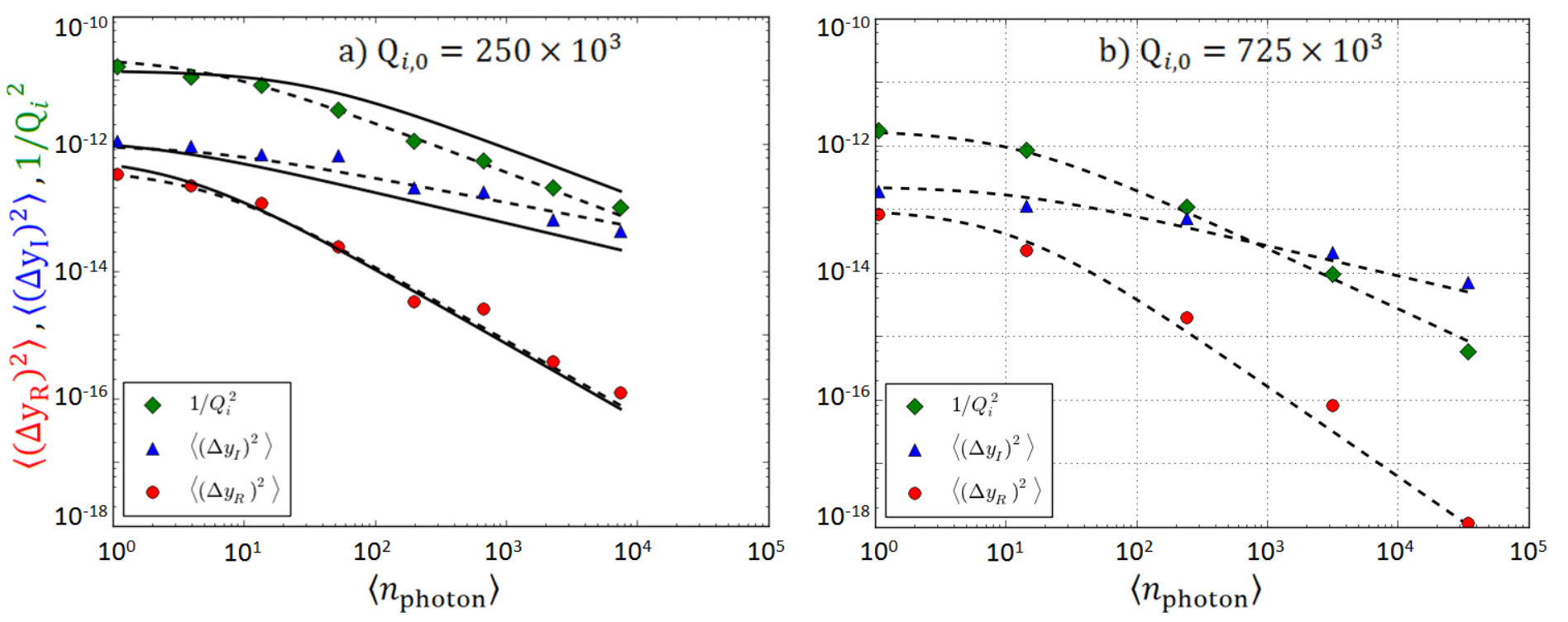
We can compare these predictions with our measurements by calculating the variances in the real and imaginary parts of the measured dimensionless admittance, and . These variances are calculated by integrating the component of the measured power spectral densities in Fig. 3. We approximate the full integrals by numerically cutting off the integrals below 1 mHz and above 5 kHz; the results only depend on the logarithmic ratio of these cutoffs. The calculated variances are plotted as a function of resonator photon occupation number in Fig. 4.
We compare the measured dependence of the squared loss , and the variances and , with the model predictions. The power-dependent loss can be scaled to match well to the dispersive fluctuations in . The power dependence of loss cubed, , is also seen to match well to the dissipative fluctuations in , as expected (we note that the relative magnitude of the dispersive and dissipative variances differs from one another by a factor of 2 at low power). We see that at single photon excitations, ; the loss fluctuates by almost 20% of its mean value. We observe similar behavior for a device with an internal quality factor that is roughly 3 times greater; this device displays roughly an order of magnitude lower variance, in agreement with the model, which scales as .
Assuming that the model variance is of order 1, Eq. (5) and the measured fractional variance imply that a relatively small equivalent number of TLSs, approximately 30, are affecting the device performance. Smaller values of would imply fewer TLSs: as we do not yet observe single fluctuators, seems to be a reasonable estimate.
The contribution of different TLSs to the overall admittance is weighted by the local electric field, which we ignored in our previous TLS model. To better understand this dependence, we used a finite element electromagnetic simulation to calculate the TLS contribution as a function of TLS location and local . We model a thin (3 nm thick) uniformly lossy dielectric with a relative permittivity of on all of the device interfaces (see Ref. 18). Using the simulated electric fields, we calculate the percentage contribution to dissipation and noise as a function of distance from the substrate-electrode corners, shown in Table 1. The contribution to the overall loss from a small volume scales as , and the local field scales with distance from the edge of a metal film as , resulting in loss contributions that are distributed logarithmically. The contribution to the overall variance, however, scales with the square of the loss, i.e. , resulting in contributions dominated by the corners.
| 0 - 10 nm | 10 - 100 nm | .1 - 1 m | 1 - 10 m | |
|---|---|---|---|---|
| Loss | 29% | 28% | 30% | 13% |
| Noise | 88% | 11% | 1% | <1% |
In Fig. 4(a) we plot the simulated power dependence of the loss squared, , and fluctuations in , , as solid lines overlaying the experimental data. Closest agreement between data and simulation is seen by setting the TLS saturation field to 10.0 V/m, the intrinsic loss tangent to and the TLS density to m3. These values agree with previous measurements [19, 10, 20] and the resulting power dependence and number of TLSs are in good agreement with the data.
In conclusion, we have shown measurements of power-dependent fluctuations in the loss and resonance frequency of superconducting resonators. We have presented a model that reproduces the measured power dependence and scaling with internal loss. From these measurements we were able to estimate the number of defects that contributed to the resonator fluctuations. The response of these devices appear to be dominated by a few dozen TLSs.
Acknowledgements.
Devices were made at the UC Santa Barbara Nanofabrication Facility, a part of the NSF-funded National Nanotechnology Infrastructure Network. This research was funded by the Office of the Director of National Intelligence (ODNI), Intelligence Advanced Research Projects Activity (IARPA), through Army Research Office grant W911NF-09-1-0375.References
- [1] A. Galiautdinov, A. Korotkov, and J. Martinis, Phys. Rev. A 85, 042321 (2012).
- [2] M. Mariantoni et al., Science 334, 61 (2011).
- [3] P. Day, H. LeDuc, B. Mazin, A. Vayonakis, and J. Zmuidzinas, Nature 425, 817 (2003).
- [4] B. Mazin et al., Opt. Express 20, 1503 (2012).
- [5] W. Phillips, Rep. Prog. Phys. 50, 1657 (1999).
- [6] J. Gao et al., Appl. Phys. Lett. 92, 152505 (2008).
- [7] R. Barends et al., Appl. Phys. Lett. 97, 033507 (2010).
- [8] J. Gao et al., Appl. Phys. Lett. 92, 212504 (2008).
- [9] J. Gao et al., Appl. Phys. Lett. 98, 232508 (2011).
- [10] J. Martinis et al., Phys. Rev. Lett. 95, 210503 (2005).
- [11] J. Kline, H. Wang, S. Oh, J. Martinis, and D. Pappas, Superconductor Science and Technology 22, 015004 (2008).
- [12] M. Vissers, J. Kline, J. Gao, D. Wisbey, and D. Pappas, Appl. Phys. Lett. 100, 082602 (2012).
- [13] A. Córcoles et al., Appl. Phys. Lett. 99, 181906 (2011).
- [14] A. Megrant et al., Appl. Phys. Lett. 100, 113510 (2012).
- [15] R. Barends et al., Appl. Phys. Lett. 99, 113507 (2011).
- [16] R. Barends et al., Applied Superconductivity, IEEE Transactions on 19, 936 (2009).
- [17] For simplicity, we have ignore thermal effects from a term, as well as negative frequency terms from the counter rotating response.
- [18] J. Wenner et al., Appl. Phys. Lett. 99, 113513 (2011).
- [19] Y. Shalibo et al., Phys. Rev. Lett. 105, 177001 (2010).
- [20] H. Wang et al., Appl. Phys. Lett. 95, 233508 (2009).