Gluonic Effects on $g-2$: Holographic View

Holography, based on AdS/CFT (anti-de-Sitter space/conformal field theory) correspondence [1], has been extensively used to analyze strongly coupled gauge systems. For instance, QCD can be reformulated based on the gauge-gravity duality, either in the bottom-up approach [2, 3] modeled as a five-dimensional gauge theory defined in an AdS background, or in the top-down approach [4] starting with a stringy setting. Such models of holographic QCD have succeeded well in reproducing several important properties for QCD hadrons within a theoretically expected size of uncertainties. In particular, the bottom-up approach can be made to reproduce the QCD in the all energy region, from the high energy behavior through the operator product expansion (OPE) down to the low energy resonance physics: The correct power behaviors in OPE for the chiral condensate and the gluon condensate are realized by introduction of the bulk (chiral non-singlet) scalar field, $\Phi_{S}$, corresponding to the $\bar{q}q$ operator and (chiral singlet) bulk gluonic field, $\Phi_{G}$, respectively [5], which is contrasted to the top-down approach having high energy behavior completely different than that of QCD. The bottom-up holography so constructed can provide us with novel insights into the strong dynamics through the highly nontrivial effects of the gluonic dynamics: It reproduces nicely the known value of the gluon condensate which is otherwise zero, and the mass of $a_{1}$ meson of the right magnitude.

Such a bottom-up holographic QCD model having gluon condensation effects (hereafter, we will use the phrase “gluonic effects” to refer to the gluon condensation effects) $\Phi_{G}$ was further applied [5] to the Walking Technicolor (WTC) model [7] which has an approximate scale symmetry and a large anomalous dimension $\gamma_{m}=1$, and further predicts a light composite Higgs dubbed “Technidilaton (TD)” as a pseudo Nambu-Goldstone boson of the approximate scale symmetry. The holographic WTC of Ref. [5] was formulated through a simple replacement of $\gamma_{m}=0$ for QCD by $\gamma_{m}=1$ in the mass parameter of the bulk scalar $\Phi_{S}$ in the holographic QCD with $\Phi_{G}$, which was found [6] to have more intriguing gluonic effects than in those of the holographic QCD: Large gluonic effects due to $\Phi_{G}$ in WTC actually realize an idealized limit where TD [7, 8] as a flavor-singlet scalar fermionic bound state (lowest Kaluza-Klein (KK) mode of $\Phi_{S}$)^#1#1 #1 Note that a scalar techni-glueball as the lowest KK mode of $\Phi_{G}$ has no direct relevance to the electroweak symmetry breaking, since the technigluons carry no electroweak charge, and hence cannot be identified with the TD, or composite Higgs, whose constituents must carry the electroweak charge. has a vanishingly small mass compared with the typical symmetry breaking scale $4\pi F_{\pi}$ ($F_{\pi}$: techni-pion decay constant), and hence it can naturally be as light as 125 GeV to be identified as the Higgs boson discovered at the LHC [9]. This is in sharp contrast to the earlier nonperturbative studies based on the ladder approximation [10, 11] without nonperturbative gluonic dynamics, which yields a substantially smaller scalar mass than in the QCD case, though it does not have such an idealized massless limit and hence no natural framework for the light TD ^#2#2 #2 We actually have a formal limit of massless TD through the ladder estimate for the Partially Conserved Dilatation Current (PCDC) relation, which involves mass $M_{\phi}$ and the decay constant $F_{\phi}$ of the TD $\phi$ only in the form of a product, $M_{\phi}F_{\phi}={\cal O}(F_{\pi}^{2})$, (not separately). This implies that a massless TD limit $M_{\phi}/F_{\pi}\rightarrow 0$ is formally realized only when $F_{\phi}/F_{\pi}\rightarrow\infty$, or the coupling vanishes (decoupled dilaton) [5, 12]. Nevertheless, it so happened that the mass estimated by the ladder PCDC actually can be parametrically tuned to be 125 GeV in such a way as to be consistent with the current LHC data, being still far from the decoupling limit [13]. . Therefore, proper inclusion of gluonic effects is important not only for the study of QCD, but also, or more significantly, for the realistic WTC calculations.

Holographic computations are generically done through evaluating Green functions constructed from (techni-)quark and gluon currents, so that the main outputs are made from the current correlators, including full information on masses and couplings for the associated mesons and glueball coupled to those currents. Once the vector current correlator is obtained from the holographic calculation, it is possible to translate it into the electromagnetic current correlator, $\Pi_{\rm em}(Q^{2})$, from which we can estimate the (techni-)hadronic leading order (HLO) contribution to the anomalous magnetic moment of the muon (the muon $g-2$). Actually, in Ref. [14] a holographic estimation of such a QCD HLO contribution was done based on an earlier bottom-up holographic model [3], in which, however, effects from the gluon condensation are not incorporated.

In this paper, we study the gluonic effects on the muon $g-2$ in QCD and WTC through the (techni-)HLO contribution, based on a recently published holographic model in the bottom-up approach [5, 6]. The model has 3 holographic parameters ($z_{m},\,\xi,\,G$) to be explained later; $\xi$ and $G$, roughly corresponding to the chiral condensate and the gluon condensate, respectively, at the infrared brane located at $z_{m}$. By fixing the values $f_{\pi}=92.4$ MeV and $M_{\rho}=775.49$ MeV as inputs, we have $\xi$ and $z_{m}$ as functions of $G$. Accordingly, we show all other hadronic observables given as functions of a single holographic gluonic parameter $G$: While the mass of the flavor-singlet scalar $f_{0}(1370)$ and the scalar glueball are insensitive to the value of $G$, the mass of $a_{1}$ meson and the gluon condensate which are fairly sensitive to $G$ so that we can determine the value of $G\simeq 0.25$ nicely fitting the reality of all the observables studied [5, 6].

We then estimate the HLO contributions including the gluon-condensation effect, based on a formula for the HLO directly evaluated by the current correlator in the (theoretically more tractable) space-like momentum in contrast to the conventional one converting it to the dispersion integral from the time-like contributions where the experimental data are available. The results show that the proper inclusion of gluon-condensation effect $G\simeq 0.25$ causes about 6% enhancement of the HLO contribution to the muon $g-2$: $a_{\mu}^{\rm HLO}|_{N_{f}=2}\simeq 505\times 10^{-10}$, $a_{\mu}^{\rm HLO}|_{N_{f}=3}\simeq 606\times 10^{-10}$, which are compared to the previous calculation [14] without gluon-condensation effect $G=0$: $a_{\mu}^{\rm HLO}|_{N_{f}=2}\simeq 476\times 10^{-10}$, $a_{\mu}^{\rm HLO}|_{N_{f}=3}\simeq 571\times 10^{-10}$, respectively. This enhancement makes the prediction of holographic calculation of the HLO contribution very close to the known value [15] from the phenomenological estimate using the experimental inputs $a_{\mu}^{\rm HLO}|_{\pi^{+}\pi^{-}}=(504.2\pm 3.0)\times 10^{-10}$ and $a_{\mu}^{\rm HLO}|_{\rm full}=(694.9\pm 4.3)\times 10^{-10}$, respectively. We also calculate the HLO contributions to the electron and the tau lepton $g-2$, and show that the holographic predictions are quite consistent with the known values as well.

Considering the fact that the energy scales important for determining the HLO effects are hierarchically different depending on the lepton species, it is remarkable that the holographic calculations, with proper inclusion of gluon-condensation effect, can reproduce HLO contributions to $g-2$ for all the leptons. This means that with inclusion of the gluonic contributions the holographic calculation of $\Pi_{\rm em}(Q^{2})$ is quite reliable in a wide range of energy scale, and remarkably in the (theoretically tractable) continuous space-like momentum, not just in the range of the (discrete) time-like momentum where the resonance parameters are fitted in the conventional holographic studies in the zero-width approximation (large $N_{c}$ limit).

Encouraged by this success, we apply the same holographic calculations of the HLO-type contributions to the $g-2$ from the WTC, with $\gamma_{m}=0$ in QCD simply replaced by $\gamma_{m}=1$ through the bulk scalar mass. We first show the gluonic effects on various observables in WTC, including the mass of the flavor-singlet scalar meson $M_{\phi}$ identified with TD, which can be as light as the 125 GeV boson discovered at the LHC for a large gluonic effect with $G\simeq 10$ [6]. Then we study the effect of such a large $G$ on the muon $g-2$ through the techni-HLO contribution, which we find as large as 100 times of the value for $G=0$: Imposing a typical constraint on the Peskin-Takeuchi $S$ parameter [16] from the electroweak (EW) precision test, $S=0.1$, the enhancement is about 10 times and by relaxing the constraint on $S$ parameter as $0.1<S<1.0$ for the reason described in the text, the techni-HLO contribution can be further enhanced by another factor of about 10. For all such enhancements, however, we show that the techni-HLO contributions from WTC dynamics is negligibly small compared to the HLO contributions from QCD. It is then very unlikely that the contributions from WTC dynamics can explain the inconsistency by about 3.3 $\sigma$ between the experimental value of the muon $g-2$ and the Standard Model (SM) prediction of it. We also mention the techni-HLO contribution to the tau $g-2$, which may become relevant in future experiments.

The paper is organized as follows: In the next section, we review the model [5] and formulas which are needed for the calculations of various physical quantities studied in this paper. In section III, we study the gluonic effect of the muon $g-2$ through the holographic QCD calculation of HLO contribution, based on the successful inclusion of the gluonc effects on the various hadonic observables in Ref. [5]. In section IV, we use similar holographic calculations for the study of WTC effects on the $g-2$. Section V is devoted to discussions and summary of the paper.

The model [5] we shall employ is based on deformations of a bottom-up approach for successful holographic dual of QCD [2, 3]. The model is described as $SU(N_{f})_{L}\times SU(N_{f})_{R}$ gauge theory defined on the five-dimensional AdS space-time, which is characterized by the metric $ds^{2}=g_{MN}dx^{M}dx^{N}=\left(L/z\right)^{2}\big(\eta_{\mu\nu}dx^{\mu}dx^{\nu}-dz^{2}\big)$ with $\eta_{\mu\nu}={\rm diag}[1,-1,-1,-1]$. Here, $M$ and $N$ ($\mu$ and $\nu$) represent five-dimensional (four-dimensional) Lorentz indices, and $L$ denotes the curvature radius of the AdS background. The fifth direction, denoted as $z$, is compactified on an interval extended from the ultraviolet (UV) brane located at $z=\epsilon$ to the infrared (IR) brane at $z=z_{m}$, i.e., $\epsilon\leq z\leq z_{m}$. The UV cutoff $\epsilon$ will be taken to be 0 after all calculations are done. In addition to the bulk left- ($L_{M}$) and right- ($R_{M}$) gauge fields, we introduce a bulk scalar $\Phi_{S}$ which transforms as a bifundamental representation field under the $SU(N_{f})_{L}\times SU(N_{f})_{R}$ gauge symmetry, and therefore it is considered to be dual to the quark bilinear operator $\bar{q}q$. The mass-parameter $m_{\Phi_{S}}$ is then related to $\gamma_{m}$ as

$$m_{\Phi_{S}}^{2}=-\frac{(3-\gamma_{m})(1+\gamma_{m})}{L^{2}}\,.$$

(1)

We take $\gamma_{m}=0$ when we apply this holographic model to the study of the actual QCD, while we take $\gamma_{m}=1$ when we consider the model as a dual of WTC. The action of the model is given as  [5]

$$S_{5}=S_{\rm bulk}+S_{\rm UV}+S_{\rm IR}\,,$$

(2)

where $S_{\rm bulk}$ denotes the five-dimensional bulk action,

	$\displaystyle S_{\rm bulk}$	$\displaystyle=$	$\displaystyle\int d^{4}x\int_{\epsilon}^{z_{m}}dz\sqrt{g}\frac{1}{g_{5}^{2}}\,e^{c_{G}g_{5}^{2}\Phi_{G}}\Bigg[\frac{1}{2}\partial_{M}\Phi_{G}\partial^{M}\Phi_{G}$		(3)
			$\displaystyle+{\rm Tr}[D_{M}\Phi_{S}^{\dagger}D^{M}\Phi_{S}-m_{\Phi_{S}}^{2}\Phi_{S}^{\dagger}\Phi_{S}]$
			$\displaystyle-\frac{1}{4}{\rm Tr}[L_{MN}L^{MN}+R_{MN}R^{MN}]\Bigg]\,,$

and $S_{\rm UV,IR}$ the boundary actions which are given in Ref. [6]. The covariant derivative acting on $\Phi_{S}$ in Eq.(3) is defined as $D_{M}\Phi_{S}=\partial_{M}\Phi_{S}+iL_{M}\Phi_{S}-i\Phi_{S}R_{M}$, where $L_{M}(R_{M})\equiv L_{M}^{a}(R_{M}^{a})T^{a}$ with $T^{a}$ being the generators of $SU(N_{f})$ which are normalized as ${\rm Tr}[T^{a}T^{b}]=\delta^{ab}$. $L(R)_{MN}$ is the five-dimensional field strength which is defined as $L(R)_{MN}=\partial_{M}L(R)_{N}-\partial_{N}L(R)_{M}-i[L(R)_{M},L(R)_{N}]$, and $g$ is defined as $g={\rm det}[g_{MN}]=(L/z)^{10}$. A salient feature of the model is the extra bulk scalar $\Phi_{G}$ introduced in Eq.(3) in order to reproduce the correct asymptotic behavior of the QCD. This is a bulk field which is dual to the gluon condensate $\langle\alpha_{s}G_{\mu\nu}^{2}\rangle$ in QCD. Here, $\alpha_{s}$ is related to the QCD gauge couping $g_{s}$ by $\alpha_{s}=g^{2}_{s}/(4\pi)$. Since $\langle\alpha_{s}G_{\mu\nu}^{2}\rangle$ is a singlet under the chiral $SU(N_{f})_{L}\times SU(N_{f})_{R}$ symmetry, the dual-bulk scalar $\Phi_{G}$ has to be a real field. We take ${\rm dim}(\alpha_{s}G_{\mu\nu}^{2})=4$, thus the corresponding bulk-mass parameter becomes $m_{\Phi_{G}}^{2}=0$. The gauge coupling $g_{5}$ and a parameter $c_{G}$ appearing in the action are fixed as

$$\frac{L}{g_{5}^{2}}=\frac{N_{c}}{12\pi^{2}},\quad c_{G}=-\frac{L}{16\pi g_{5}^{2}}=-\frac{N_{c}}{192\pi^{3}}\,,$$

(4)

so that the model reproduces the OPE in QCD (see later discussions) [5].

We shall begin with the bulk scalar sector in Eq.(3). The bulk scalar fields $\Phi_{S}$ and $\Phi_{G}$ are parametrized as

$$\Phi_{S}(x,z)=\frac{1}{\sqrt{2}}\left(v_{S}(z)+\frac{\sigma_{S}(x,z)}{\sqrt{N_{f}}}\right)e^{2i\pi(x,z)/v_{S}(z)},$$

(5)

$$\chi_{G}(x,z)\equiv e^{c_{G}g_{5}^{2}\Phi_{G}/2}=v_{\chi_{G}}(z)\,e^{\sigma_{\chi_{G}}(x,z)/v_{\chi_{G}}(z)},$$

(6)

with the vacuum expectation values (VEVs), $v_{S}=\sqrt{2}\langle\Phi_{S}\rangle$ and $v_{\chi_{G}}=\langle\chi_{G}\rangle$. We hereafter disregard (techni-)pion fields $\pi$ which will not be relevant for the present study. The boundary conditions for $v_{S}(z)$ are [17, 5, 6]:

	$\displaystyle v_{S}(\epsilon)$	$\displaystyle=$	$\displaystyle\Bigg\{\begin{array}[]{cc}\left(\frac{\epsilon}{L}\right)\,c_{S}^{\gamma_{m}=0}M&\quad\textrm{for}\quad\gamma_{m}=0\\ \left(\frac{\epsilon}{L}\right)^{2}\log\frac{z_{m}^{2}}{\epsilon^{2}}\,c_{S}^{\gamma_{m}=1}M&\quad\textrm{for}\quad\gamma_{m}=1\end{array}\,,$
	$\displaystyle v_{S}(z_{m})$	$\displaystyle=$	$\displaystyle\frac{\xi}{L}\,,$		(10)

where $M$ stands for the current mass of (techni-)quarks, and the IR value $\xi$ is related to the (techni-)quark condensate $\langle\bar{q}q\rangle$. The parameter $c_{S}^{\gamma_{m}}$ has been introduced which can arise from the ambiguity of the definition for the current mass $M$, and is fixed to be $c_{S}^{\gamma_{m}=0}=\sqrt{3}$ for QCD and $c_{S}^{\gamma_{m}=1}=\sqrt{3}/2$ for WTC, by matching the UV asymptotic form of the scalar current correlator to the form predicted from the operator product expansion [6].

The boundary conditions for $v_{\chi_{G}}(z)$ are taken for both QCD and WTC cases as

	$\displaystyle v_{\chi_{G}}(\epsilon)$	$\displaystyle=$	$\displaystyle e^{\frac{c_{G}}{2}\frac{g_{5}^{2}}{L}M^{\prime}}=e^{-\frac{1}{32\pi}LM^{\prime}}\,,$		(11)
	$\displaystyle v_{\chi_{G}}(z_{m})$	$\displaystyle=$	$\displaystyle 1+G\,,$		(12)

where $M^{\prime}$ becomes an external source for the (techni-)gluon condensate operator $(\alpha_{s}G^{2}_{\mu\nu})$, and $G$ is a parameter which is associated with the (techni-)gluon condensate $\langle\alpha_{s}G_{\mu\nu}^{2}\rangle$. The solutions of the VEVs $v_{S}(z)$ and $v_{\chi_{G}}(z)$ in the limit where $M\to 0$ and $M^{\prime}\to 0$ are given as [5]

	$\displaystyle v_{S}(z)$	$\displaystyle=$	$\displaystyle\Bigg\{\begin{array}[]{cc}\frac{\xi(1+G)}{L}\frac{(z/z_{m})^{3}}{1+G(z/z_{m})^{4}}&\quad\textrm{for}\quad\gamma_{m}=0\\ \frac{\xi(1+G)}{L}\frac{(z/z_{m})^{2}}{1+G(z/z_{m})^{4}}\frac{\log(z/\epsilon)}{\log(z_{m}/\epsilon)}&\quad\textrm{for}\quad\gamma_{m}=1\end{array}$
	$\displaystyle v_{\chi_{G}}(z)$	$\displaystyle=$	$\displaystyle 1+G\left(\frac{z}{z_{m}}\right)^{4}\,.$		(16)

One can solve the equations of motion for the bulk scalars $\sigma_{S}$ and $\sigma_{\chi_{G}}$ with the UV boundary conditions similar to those in Eqs. (II) and (11) with $M$ and $M^{\prime}$ replaced by sources $(s(x),g(x))$ for the scalar and gluonic currents $(J_{S}(x),J_{G}(x))$. Putting their solutions back into the action $S_{5}$ in Eq.(2), one can then obtain the generating functional $W[s(x),g(x)]$ holographically dual to QCD or WTC. The chiral condensate and gluon condensate ($\langle\bar{q}q\rangle$ and $\langle\alpha_{s}G^{2}_{\mu\nu}\rangle$) are thus calculated by performing $\delta W/\delta s(x)$ and $\delta W/\delta g(x)$, respectively:

	$\displaystyle\langle\bar{q}q\rangle_{1/z_{m}}$	$\displaystyle=$	$\displaystyle-\frac{c_{S}^{\gamma_{m}}(3-\gamma_{m})N_{c}}{12\pi^{2}}\frac{\xi(1+G)}{z_{m}^{3}}\,,\qquad c_{S}^{\gamma_{m}}=\Bigg\{\begin{array}[]{cc}\sqrt{3}&\qquad{\rm for}\qquad\gamma_{m}=0\\ \sqrt{3}/2&\qquad{\rm for}\qquad\gamma_{m}=1\end{array}\,,$
	$\displaystyle\langle\alpha_{s}G^{2}_{\mu\nu}\rangle$	$\displaystyle=$	$\displaystyle\frac{32N_{c}}{3\pi}\frac{G}{z_{m}^{4}}\,,$		(20)

where $\langle\bar{q}q\rangle_{1/z_{m}}$ is the chiral condensate renormalized at $\mu=1/z_{m}$ [17]. The chiral condensate renormalized at generic scale $\mu$ is given by $\langle\bar{q}q\rangle_{\mu}=Z_{m}^{-1}(\mu z_{m})\cdot\langle\bar{q}q\rangle_{1/z_{m}}$ with $Z_{m}^{-1}(\mu z_{m})=(\mu z_{m})^{\gamma_{m}}$. One can also calculate the scalar meson (TD) mass $M_{S}$ and glueball mass $M_{G}$ by evaluating the lowest poles of the scalar and gluonic current correlators [6] to find the following eigenvalue equations:

	$\displaystyle M_{S}$	$\displaystyle:$	$\displaystyle\frac{3}{2}\xi^{2}J_{1-\gamma_{m}}(M_{S}z_{m})=(M_{S}z_{m})J_{2-\gamma_{m}}(M_{S}z_{m}),$		(21)
	$\displaystyle M_{G}$	$\displaystyle:$	$\displaystyle J_{1}(M_{G}z_{m})=0\,,$		(22)

where $J$ is the Bessel function of the first kind.

We shall move on to the gauge sector in Eq.(3). We define the five-dimensional vector and axial-vector gauge fields $V_{M}$ and $A_{M}$ as

$$V_{M}=\frac{L_{M}+R_{M}}{\sqrt{2}}\,,\qquad A_{M}=\frac{L_{M}-R_{M}}{\sqrt{2}}\,.$$

(23)

It is convenient to work with the gauge-fixing $V_{z}=A_{z}\equiv 0$ and take the boundary conditions $V_{\mu}(x,\epsilon)=v_{\mu}(x)$, $A_{\mu}(x,\epsilon)=a_{\mu}(x)$ and $\partial_{z}V_{\mu}(x,z)|_{z=z_{m}}=\partial_{z}A_{\mu}(x,z)|_{z=z_{m}}=0$, where $v_{\mu}(x)$ and $a_{\mu}(x)$ correspond to sources for the vector and axial-vector currents, respectively. We then solve the equations of motion for (the transversely polarized components of) $V_{\mu}(x,z)$ and $A_{\mu}(x,z)$ and substitute the solutions back into the action in Eq.(3), to obtain the generating functional $W[v_{\mu},a_{\mu}]$ holographically dual to QCD or WTC. Then the vector and the axial-vector current correlators are obtained in a way similar to the case of the scalar sector. The correlators are defined as

	$\displaystyle i\int d^{4}xe^{iqx}\langle 0|\,{\rm T}\,J_{V}^{a\mu}(x)\,J_{V}^{b\nu}(0)\,|0\rangle$	$\displaystyle=$	$\displaystyle\delta^{ab}\left(\frac{q^{\mu}q^{\nu}}{q^{2}}-\eta^{\mu\nu}\right)\Pi_{V}(-q^{2}),$		(24)
	$\displaystyle i\int d^{4}xe^{iqx}\langle 0|\,{\rm T}\,J_{A}^{a\mu}(x)\,J_{A}^{b\nu}(0)\,|0\rangle$	$\displaystyle=$	$\displaystyle\delta^{ab}\left(\frac{q^{\mu}q^{\nu}}{q^{2}}-\eta^{\mu\nu}\right)\Pi_{A}(-q^{2}),$		(25)

where the currents are defined as

	$\displaystyle J_{V}^{a\mu}$	$\displaystyle=$	$\displaystyle\bar{\psi}\left(\frac{T^{a}}{\sqrt{2}}\right)\gamma^{\mu}\psi,$		(26)
	$\displaystyle J_{A}^{a\mu}$	$\displaystyle=$	$\displaystyle\bar{\psi}\left(\frac{T^{a}}{\sqrt{2}}\right)\gamma^{\mu}\gamma_{5}\psi.$		(27)

$\Pi_{V}(Q^{2})$ and $\Pi_{A}(Q^{2})$ (where $Q\equiv\sqrt{-q^{2}}$ is the Euclidean momentum) are expressed as

	$\displaystyle\Pi_{V}(Q^{2})$	$\displaystyle=$	$\displaystyle\frac{N_{c}}{12\pi^{2}}\frac{\partial_{z}V(Q^{2},z)}{z}\Bigg|_{z=\epsilon\to 0}\,,$		(28)
	$\displaystyle\Pi_{A}(Q^{2})$	$\displaystyle=$	$\displaystyle\frac{N_{c}}{12\pi^{2}}\frac{\partial_{z}A(Q^{2},z)}{z}\Bigg|_{z=\epsilon\to 0}\,,$		(29)

where the vector and axial-vector profile functions $V(Q^{2},z)$ and $A(Q^{2},z)$ are defined as $V_{\mu}(q,z)=v_{\mu}(q)V(q^{2})$ and $A_{\mu}(q,z)=a_{\mu}(q)A(q^{2})$ with the Fourier transforms of $v_{\mu}(x)$ and $a_{\mu}(x)$. These profile functions satisfy the following equations:

$$\left[-Q^{2}+\omega^{-1}(z)\partial_{z}\omega(z)\partial_{z}\right]V(Q^{2},z)=0,$$

(30)

$$\left[-Q^{2}+\omega^{-1}(z)\partial_{z}\omega(z)\partial_{z}-2\left(\frac{L}{z}\right)^{2}[v_{S}(z)]^{2}\right]A(Q^{2},z)=0,$$

(31)

$$\omega(z)\equiv\frac{L}{z}\left(1+G\left(\frac{z}{z_{m}}\right)^{4}\right)^{2}\,,$$

(32)

with the boundary conditions $V(Q^{2},z)|_{z=\epsilon\rightarrow 0}=A(Q^{2},z)|_{z=\epsilon\rightarrow 0}=1$ and $\partial_{z}V(Q^{2},z)|_{z=z_{m}}=\partial_{z}A(Q^{2},z)|_{z=z_{m}}=0$. It is worth mentioning that both the vector and the axial-vector current correlators involve gluonic effects through $G$. Most notably, we have

$$\Pi_{V}(Q^{2})\Bigg|_{(1/z_{m})^{2}\ll Q^{2}<(1/\epsilon)^{2}}=Q^{2}\left[~\frac{L}{2g_{5}^{2}}\log{Q^{2}}+c_{G}\frac{2}{3}\frac{g_{5}^{2}}{L}\frac{\langle\alpha_{s}G_{\mu\nu}^{2}\rangle}{Q^{4}}+\cdots~\right]\,,$$

(33)

in accord with the OPE in QCD:

$\displaystyle\Pi_{V}^{(\rm QCD)}\left(Q^{2}\right)\Bigg|_{\rm OPE}$

$\displaystyle=$

$\displaystyle Q^{2}\left[\frac{N_{c}}{24\pi^{2}}\log\left(\frac{Q^{2}}{\mu^{2}}\right)-\frac{1}{24\pi}\frac{\langle\alpha_{s}G_{\mu\nu}^{2}\rangle}{Q^{4}}+\cdots\right]\,,$

(34)

which was the basis for the parameter matching in Eq.(4). Were it not for the $\Phi_{G}$ term, we would not reproduce the correct gluon condensate term $1/Q^{4}$ in the QCD asymptotics and also in WTC. Therefore the physical quantities which are related to these correlators, including the muon $g-2$, are influenced by the existence of gluonic dynamics.

The vector and axial-vector current correlators, $\Pi_{V}$ and $\Pi_{A}$, can be expanded in terms of towers of the vector and axial-vector resonances. We then identify the lowest poles for $\Pi_{V,A}$ as the (techni-)$\rho$ and $a_{1}$ mesons. Their masses, $M_{\rho}$ and $M_{a_{1}}$, are calculated by solving the eigenvalue equations for the vector and axial-vector profile functions [5]:

$$\left[M_{\rho}^{2}+\omega^{-1}(z)\partial_{z}\omega(z)\partial_{z}\right]V(z)=0,$$

(35)

$$\left[M_{a_{1}}^{2}+\omega^{-1}(z)\partial_{z}\omega(z)\partial_{z}-2\left(\frac{L}{z}\right)^{2}[v_{S}(z)]^{2}\right]A(z)=0,$$

(36)

with the same boundary conditions $V(\epsilon)=A(\epsilon)=0$ and $\partial_{z}V(z)|_{z=z_{m}}=\partial_{z}A(z)|_{z=z_{m}}=0$. We thus find $M_{\rho}$ and $M_{a_{1}}$ as functions of the model parameters $\xi$, $G$ and $\gamma_{m}$ with the overall scale set by $z_{m}$: $M_{\rho}=z_{m}^{-1}\cdot\widetilde{M}_{\rho}(G)$ and $M_{a_{1}}=z_{m}^{-1}\cdot\widetilde{M}_{a_{1}}(\xi,G,\gamma_{m})$.

The (techni-)pion decay constant is expressed as $f_{\pi}^{2}=\Pi_{V}(0)-\Pi_{A}(0)$, which is, in the case of WTC, related to the EW scale $v_{\rm EW}\simeq 246$ GeV as $F_{\pi}=v_{\rm EW}/\sqrt{N_{D}}$. Here, $N_{D}$ denotes the number of EW doublets, which is fixed to be 1 in the case of QCD. The present model enables us to express $f_{\pi}$ as a function of $\xi$, $G$, $\gamma_{m}$ and $z_{m}$ [5]:

$\displaystyle f_{\pi}^{2}$

$\displaystyle=$

$\displaystyle\frac{N_{c}}{12\pi^{2}}\frac{\widetilde{F}^{2}(\xi,G,\gamma_{m})}{z_{m}^{2}}\,,$

(37)

where $\widetilde{F}^{2}=-\partial_{t}A(Q^{2}=0,t=z/z_{m})/t|_{t=\epsilon/z_{m}\to 0}$.

The $S$ parameter [16] is calculated from $\Pi_{V}$ and $\Pi_{A}$ as $S=-16\pi L_{10}=-4\pi\,N_{D}\left[\Pi^{\prime}_{V}(0)-\Pi^{\prime}_{A}(0)\right]$, where $\Pi^{\prime}_{V,A}(0)\equiv d\Pi_{V,A}(Q^{2})/dQ^{2}|_{Q^{2}=0}$. Thus $S$ is expressed as a function of two parameters $\xi$ and $G$ [5] once $\gamma_{m}$ is fixed:

$\displaystyle S=-16\pi L_{10}=\frac{N_{D}N_{c}}{3\pi}\int_{t_{\epsilon}}^{1}\frac{dt}{t}v_{\chi}^{2}(t)\left(1-[A(Q^{2}=0,t=z/z_{m})]^{2}\right)\,,$

(38)

where $t_{\epsilon}=\epsilon/z_{m}(\to 0)$.

Once $\Pi_{V}(Q^{2})$ is calculated in the holographic model, the electromagnetic current correlator $\Pi_{\rm em}(Q^{2})$ is obtained as

$$\Pi_{\rm em}(Q^{2})=2\left(\sum_{f}q_{f}^{2}\right)\frac{\Pi_{V}(Q^{2})}{Q^{2}},$$

(39)

where the summation runs over all the fermion flavors $f$ with their electromagnetic charge denoted as $q_{f}$. Here, we defined electromagnetic current correlator as

$$i\int d^{4}xe^{iqx}\langle 0|\,{\rm T}\,J_{\rm em}^{\mu}(x)\,J_{\rm em}^{\nu}(0)\,|0\rangle=\left(q^{2}\eta^{\mu\nu}-q^{\mu}q^{\nu}\right)\Pi_{\rm em}(-q^{2}),$$

(40)

where the electromagnetic current is defined as $J_{\rm em}^{\mu}=\sum_{f}q_{f}\bar{\psi}_{f}\gamma^{\mu}\psi_{f}$. With the electromagnetic current correlator given, the (techni-)hadronic leading order (HLO) contribution to the muon $g-2$ is calculated to be [18] (For a graphical expression, see Fig. 1.)

$$\left.\left(\frac{g-2}{2}\right)\right|_{{\rm(techni)HLO}}\equiv a_{\mu}^{\rm(techni)HLO}=4\pi^{2}\left(\frac{\alpha_{\rm em}}{\pi}\right)^{2}\int_{0}^{\infty}dQ^{2}f(Q^{2})\Pi_{\rm em}^{R}(Q^{2})\,,$$

(41)

where $\alpha_{\rm em}=e^{2}/(4\pi)$ with $e$ being the electromagnetic coupling constant. $\Pi_{\rm em}^{R}(Q^{2})$ is the renormalized electromagnetic current correlator defined as $\Pi_{\rm em}^{R}(Q^{2})\equiv\Pi_{\rm em}(Q^{2})-\Pi_{\rm em}(0)$, and $f(Q^{2})$ is a weight function which has the following form:

	$\displaystyle f(Q^{2})$	$\displaystyle=$	$\displaystyle\frac{m_{\mu}^{2}Q^{2}Z^{3}(1-Q^{2}Z)}{1+m_{\mu}^{2}Q^{2}Z^{2}}\,,$
	$\displaystyle Z$	$\displaystyle\equiv$	$\displaystyle\frac{\sqrt{Q^{4}+4m_{\mu}^{2}Q^{2}}-Q^{2}}{2m_{\mu}^{2}Q^{2}}.$		(42)

The formula can be rewritten in terms of $\Pi_{V}$ as follows:

$$a_{\mu}^{\rm(techni-)HLO}=4\pi^{2}\left(\frac{\alpha_{\rm em}}{\pi}\right)^{2}{\cal N}\int_{0}^{\infty}\frac{dQ^{2}}{Q^{2}}f(Q^{2})\left(\Pi_{V}(Q^{2})-\Pi_{V}(0)\right),$$

(43)

where ${\cal N}$ is the prefactor in Eq. (39), which takes the following values in the case of QCD and one-family technicolor model [19]:

$\displaystyle{\cal N}\equiv 2\sum_{f}q_{f}^{2}=\left\{\begin{array}[]{l}10/9\ \ \ {\rm QCD}\ (N_{f}=2)\\ \ 4/3\ \ \ \,{\rm QCD}\ (N_{f}=3)\\ 16/3\ \ \ \textrm{one-family technicolor}\end{array}\right.$

Now, all the physical quantities we are interested in have been expressed in terms of calculable holographic quantities. In the following two sections, for the case of QCD and WTC respectively, we evaluate those physical quantities as functions of the model parameters $\xi,z_{m},G$ and $\gamma_{m}$, especially focusing on their dependence on $G$ closely related to the gluon condensate.

In this section, we apply the holographic calculations explained in the previous section for the estimation of various physical quantities in the real-life QCD. For this purpose, we take $\gamma_{m}=0$ so that the model correctly reproduces the UV asymptotic behavior of the QCD. After fixing the value of $\gamma_{m}$, all the physical quantities are expressed as functions of $z_{m}$, $\xi$ and $G$. We use $M_{\rho}=775.49$ MeV and $f_{\pi}=92.4$ MeV as inputs to fix two of these remaining model parameters. Then, from Eqs. (35) and (37), one can express $z_{m}$ and $\xi$ as functions of $G$. Now, the remaining physical quantities, namely $M_{a_{1}}$, $\langle\frac{\alpha_{s}}{\pi}G_{\mu\nu}^{2}\rangle$, $(-\langle\bar{q}q\rangle)^{1/3}$, $M_{S}$, $M_{G}$ and $S=-16\pi L_{10}$ can be expressed as functions of a single parameter $G$ through Eqs. (36), (II), (20), (21), (22) and (38), which are depicted in Fig. 2 by varying $G$ from 0 to 0.4:

Observed values of those quantities are also indicated in the plots: two dashed red lines correspond to upper and lower values of 1-$\sigma$ error band. The “observed” glueball mass $M_{G}$ has been taken from an expected mass range in lattice simulations [23]. As for the flavor-singlet two-quark bound state $S$ meson, we have chosen $f_{0}(1370)$ and estimated the “observed” mass neglecting mixing with four-quark bound state $f_{0}(980)$. (For more detailed discussions, see Ref. [5].)

The figures tell us that the $a_{1}$ meson mass $M_{a_{1}}$ and gluon condensate $\langle\frac{\alpha_{s}}{\pi}G_{\mu\nu}^{2}\rangle$ highly depend on the change of $G$, while other quantities are rather insensitive to it, keeping values at around observed values of each quantity. From these results, we see the optimal value of $G$ (and hence $z_{m}$ and $\xi$): [5]

$$G\simeq 0.25\,,\quad z_{m}^{-1}\simeq 347\,{\rm MeV}\,,\quad\xi\simeq 3.1\,\,,$$

(48)

for the holographic model with $\gamma_{m}=0$ to reproduce the QCD observables. In Table 1 we show the results of holographic calculations for $G=0.25$ (and $G=0$ for comparison) along with observed value of each quantity.

We see that the agreement between holographic predictions and the observed values are much improved compared with the case $G=0$. As was discussed in Ref. [5], nonzero gluonic effects with $G\simeq 0.25$ are important to achieve such a simultaneous agreement of various QCD observables, most notably $\langle\frac{\alpha_{s}}{\pi}G_{\mu\nu}^{2}\rangle$ and $M_{a_{1}}$.

Now we discuss the QCD gluonic effect on the hadronic leading order contribution to muon $g-2$, $a_{\mu}^{\rm HLO}$, which can be calculated through Eq.(43). As was done for calculations of other observables, we take $\gamma_{m}=0$, $f_{\pi}=92.4$ MeV and $M_{\rho}=775.49$ MeV as inputs, then calculate the value of $a_{\mu}^{\rm HLO}$ as a function of $G$ to see gluonic effects on it.

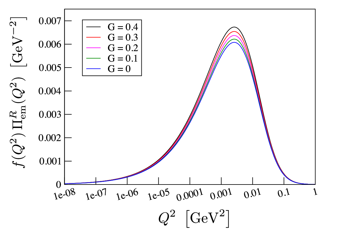
The left panel of Fig. 3 shows the integrand in Eq.(43) as a function of $Q^{2}$ varying $G$ from 0 to 0.4 with $f_{\pi}=92.4$ MeV and $M_{\rho}=775.49$ MeV fixed. We see that as $G$ increases from 0 to 0.4, the peak value at around $Q^{2}=m_{\mu}^{2}$ becomes larger, leading to the enhancement of $a_{\mu}^{\rm HLO}$. In the right panel of Fig. 3 we plot $a_{\mu}^{\rm HLO}$ as a function of $G$ for the case of $N_{f}=2$ with $f_{\pi}=92.4$ MeV and $M_{\rho}=775.49$ MeV fixed. As was expected from the enhancement of the integrand, the figure shows that the size of $a_{\mu}^{\rm HLO}$ becomes larger as $G$ increases. The values $a_{\mu}^{\rm HLO}$ at the optimal point ($G=0.25$) is estimated (in the chiral limit $m_{u}=m_{d}=m_{s}=0$) as

	$\displaystyle a_{\mu}^{\rm HLO}|_{N_{f}=2}$	$\displaystyle\simeq$	$\displaystyle 505\times 10^{-10}\qquad{\rm at}\qquad G=0.25\,,$
	$\displaystyle a_{\mu}^{\rm HLO}|_{N_{f}=3}$	$\displaystyle\simeq$	$\displaystyle 606\times 10^{-10}\qquad{\rm at}\qquad G=0.25\,.$		(49)

The predicted value for $N_{f}=2$ above is in excellent agreement with a partial hadronic contribution to $a_{\mu}^{\rm HLO}$ estimated only from $\sigma(e^{+}e^{-}\to\pi^{+}\pi^{-})$, $a_{\mu}^{\rm HLO}|_{\pi^{+}\pi^{-}}=(504.2\pm 3.0)\times 10^{-10}$ [15]. The size of $a_{\mu}^{\rm HLO}|_{N_{f}=3}$ is compared with the full hadronic contributions, $a_{\mu}^{\rm HLO}|_{\rm full}=(694.9\pm 4.3)\times 10^{-10}$ [15]. Agreements are quite impressive, considering that our estimate is only at chiral limit $m_{u}=m_{d}=m_{s}=0$.

The above results can be compared to the value of $a_{\mu}^{\rm HLO}$ obtained without gluon condensation effect [14], which can be realized by setting $G=0$:

	$\displaystyle a_{\mu}^{\rm HLO}|_{N_{f}=2}$	$\displaystyle\simeq$	$\displaystyle 476\times 10^{-10}\qquad{\rm at}\qquad G=0,$
	$\displaystyle a_{\mu}^{\rm HLO}|_{N_{f}=3}$	$\displaystyle\simeq$	$\displaystyle 571\times 10^{-10}\qquad{\rm at}\qquad G=0\,.$		(50)

We see that the inclusion of gluonic effect results in enhancement of the value of $a_{\mu}^{\rm HLO}$ by about 6%, and in both $N_{f}=2$ and $3$ cases, the agreement between holographic prediction and experimental value becomes better at $G=0.25$ compared to the results obtained from holographic model without gluonic effect.

Before closing this section, we show the results of similar holographic calculations for the HLO contribution to the anomalous magnetic moment of the electron and the tau lepton. The formulae for $a_{e}^{\rm HLO}$ and $a_{\tau}^{\rm HLO}$ can be obtained simply by replacing $m_{\mu}$ in Eq. (42) by $m_{e}$ and $m_{\tau}$, respectively. In Table 2, we show the results in the case of $N_{f}=2,3$ and $G=0,0.25$. The values for $a_{\mu}^{\rm HLO}$ are also listed as well.

The resultant value of $a_{e}^{\rm HLO}$ can be compared to the value $\sim 186.6(\pm 1.1)\times 10^{-14}$, which was obtained in Ref. [25] by using the same $e^{+}e^{-}\rightarrow$ hadrons data as those used in Ref. [15]. As for $a_{\tau}^{\rm HLO}$, it is roughly $(200-400)\times 10^{-8}$. (See, for example, Table 1 in Ref. [26] for a nice summary of various estimations of $a_{\tau}^{\rm HLO}$.) It is remarkable that the holographic predictions of the HLO contribution to $g-2$ are quite consistent with the known values for all leptons. Considering the fact that the energy scales which are important for determining $a_{e}^{\rm HLO}$, $a_{\mu}^{\rm HLO}$ and $a_{\tau}^{\rm HLO}$ are $Q^{2}\sim m_{e}^{2},m_{\mu}^{2}$ and $m_{\tau}^{2}$ respectively, the above mentioned good agreement indicates that the holographic calculation of $\Pi_{\rm em}(Q^{2})$ is quite reliable in a wide range of the continuous space-like momentum, not just in the range of the (discrete) time-like momentum where the resonance parameters are fitted in the conventional holographic studies in the zero-width approximation (large $N_{c}$ limit).

If the EW symmetry is dynamically broken by WTC, it is natural to expect that there are techni-hadronic contributions to the anomalous magnetic moment of leptons in a way analogous to the QCD HLO contributions. In this section, we estimate such effects in WTC. Throughout calculations in this section, we take $\gamma_{m}=1$ for the bulk scalar mass term, instead of $\gamma_{m}=0$ for QCD in the previous section, so that the model reproduces desired walking behavior of WTC. To be concrete, we take the one-family model[19] for the WTC as an example, in which case the number of techni-fermion is $N_{f}=8$, having $N_{D}=4$ weak doublet in the model. Actually, recent lattice results for $SU(3)$ gauge theories suggest that $N_{f}=8$ is a walking theory [27]. The techni-pion decay constant $F_{\pi}$ is related to the EW scale $v_{\rm EW}$ as $F_{\pi}=v_{\rm EW}/\sqrt{N_{D}}$, therefore, in the case of one-family WTC model, it is fixed to be $F_{\pi}=246{\rm GeV}/\sqrt{4}=123$ GeV. In order to see the dependence of physical observables on $G$ in WTC, we further fix the holographic infrared scale $z_{m}^{-1}$ at typical values $z_{m}^{-1}=2,\,4,\,6\,{\rm TeV}$, which roughly covers the phenomenologically interesting region of the $S$ parameter [16], $0.1<S<1.0$. (see discussions below).

References

- [1] J. M. Maldacena, Adv. Theor. Math. Phys. 2, 231 (1998) [Int. J. Theor. Phys. 38, 1113 (1999)].
- [2] L. Da Rold and A. Pomarol, Nucl. Phys. B 721, 79 (2005).
- [3] J. Erlich, E. Katz, D. T. Son and M. A. Stephanov, Phys. Rev. Lett. 95, 261602 (2005).
- [4] T. Sakai and S. Sugimoto, Prog. Theor. Phys. 113, 843 (2005).
- [5] K. Haba, S. Matsuzaki and K. Yamawaki, Phys. Rev. D 82, 055007 (2010).
- [6] S. Matsuzaki and K. Yamawaki, Phys. Rev. D 86, 115004 (2012).
- [7] K. Yamawaki, M. Bando and K. Matumoto, Phys. Rev. Lett. 56, 1335 (1986); M. Bando, T. Morozumi, H. So and K. Yamawaki, Phys. Rev. Lett. 59, 389 (1987).
- [8] M. Bando, K. Matumoto and K. Yamawaki, Phys. Lett. B 178, 308 (1986).
- [9] S. Chatrchyan et al. [CMS Collaboration], Phys. Lett. B 716, 30 (2012); G. Aad et al. [ATLAS Collaboration], Phys. Lett. B 716, 1 (2012).
- [10] M. Harada, M. Kurachi and K. Yamawaki, Phys. Rev. D 68, 076001 (2003); M. Kurachi and R. Shrock, JHEP 0612, 034 (2006).
- [11] S. Shuto, M. Tanabashi and K. Yamawaki, in Proc. 1989 Workshop on Dynamical Symmetry Breaking, Dec. 21-23, 1989, Nagoya, eds. T. Muta and K. Yamawaki (Nagoya Univ., Nagoya, 1990) 115-123; M. S. Carena and C. E. M. Wagner, Phys. Lett. B 285, 277 (1992); M. Hashimoto, Phys. Lett. B 441, 389 (1998).
- [12] M. Hashimoto and K. Yamawaki, Phys. Rev. D 83, 015008 (2011).
- [13] S. Matsuzaki and K. Yamawaki, Phys. Rev. D 85, 095020 (2012); Phys. Rev. D 86, 035025 (2012); Phys. Lett. B 719, 378 (2013).
- [14] D. K. Hong, D. Kim and S. Matsuzaki, Phys. Rev. D 81, 073005 (2010).
- [15] K. Hagiwara, R. Liao, A. D. Martin, D. Nomura and T. Teubner, J. Phys. G 38, 085003 (2011).
- [16] M. E. Peskin and T. Takeuchi, Phys. Rev. Lett. 65 (1990), 964; Phys. Rev. D 46 (1992), 381; B. Holdom and J. Terning, Phys. Lett. B 247 (1990), 88; M. Golden and L. Randall, Nucl. Phys. B 361 (1991), 3.
- [17] K. Haba, S. Matsuzaki and K. Yamawaki, Prog. Theor. Phys. 120, 691 (2008).
- [18] T. Blum, Phys. Rev. Lett. 91, 052001 (2003); C. Aubin and T. Blum, Phys. Rev. D 75, 114502 (2007).
- [19] E. Farhi and L. Susskind, Phys. Rev. D 20, 3404 (1979).
- [20] J. Beringer et al. [Particle Data Group Collaboration], Phys. Rev. D 86, 010001 (2012).
- [21] M. A. Shifman, A. I. Vainshtein and V. I. Zakharov, Nucl. Phys. B 147, 385 (1979); Nucl. Phys. B 147, 448 (1979).
- [22] J. Gasser and H. Leutwyler, Phys. Rept. 87, 77 (1982).
- [23] For a recent review, see W. Ochs, arXiv:1301.5183 [hep-ph].
- [24] M. Harada and K. Yamawaki, Phys. Lett. B 297, 151 (1992).
- [25] D. Nomura and T. Teubner, Nucl. Phys. B 867, 236 (2013).
- [26] S. Eidelman and M. Passera, Mod. Phys. Lett. A 22, 159 (2007).
- [27] Y. Aoki, T. Aoyama, M. Kurachi, T. Maskawa, K.-i. Nagai, H. Ohki, A. Shibata, K. Yamawaki and T. Yamazaki, Phys. Rev. D 78, 094511 (2013).
- [28] G. Cacciapaglia, C. Csaki, C. Grojean and J. Terning, Phys. Rev. D 71, 035015 (2005); R. Foadi, S. Gopalakrishna and C. Schmidt, Phys. Lett. B 606, 157 (2005); R. S. Chivukula, E. H. Simmons, H. J. He, M. Kurachi and M. Tanabashi, Phys. Rev. D 72, 016008 (2005).
- [29] G. W. Bennett et al. [Muon G-2 Collaboration], Phys. Rev. D 73, 072003 (2006).
- [30] Y. Aoki, T. Aoyama, M. Kurachi, T. Maskawa, K.-i. Nagai, H. Ohki, E. Rinaldi, A. Shibata, K. Yamawaki and T. Yamazaki, arXiv:1305.6006 [hep-lat].