Further studies on holographic insulator/superconductor phase transitions from Sturm-Liouville eigenvalue problems
Abstract
We take advantage of the Sturm-Liouville eigenvalue problem to analytically study the holographic insulator/superconductor phase transition in the probe limit. The interesting point is that this analytical method can not only estimate the most stable mode of the phase transition, but also the second stable mode. We find that this analytical method perfectly matches with other numerical methods, such as the shooting method. Besides, we argue that only Dirichlet boundary condition of the trial function is enough under certain circumstances, which will lead to a more precise estimation. This relaxation for the boundary condition of the trial function is first observed in this paper as far as we know.
pacs
11.25.Tq, 04.70.Bw, 74.20.-zI Introduction
The AdS/CFT correspondence [1, 2, 3] states that the gravity in an asymptotically AdS spacetime is dual to a field theory which sits on the boundary of the gravity. Although originally AdS/CFT correspondence was realized between a type IIB supergravity with geometry and its dual field theory with super-Yang Mills on its boundary, the AdS/CFT correspondence has been widely extended to various general cases. For example, one can have a black hole in the bulk which is corresponding to a field theory with temperature on the boundary [4]; or one can work in an asymptotic Lifshitz spacetime [5] which is dual to a non-relativistic field theory, etc. In recent years, the applications of AdS/CFT had an overwhelming development in condensed matter physics. For instance, the holographic superconductor(superfluids) phase transition [6], the holographic (non-)Fermi liquid [7, 8, 9], and holographic insulator/superconductor phase transition [10, 11, 12, 13], etc. Among these, the holographic insulator/superconductor phase transition was studied in an AdS soliton spacetime [14] which is dual to a confined gauge field theory with a mass gap on the boundary [4]. This mass gap resembles the mass gap in the insulator in condensed matter physics, which is the motivation to use AdS soliton as the background. The insulator/superconductor phase transition occurs at some critical chemical potential, beyond which the charged scalar will have a non-vanishing value which spontaneously breaks the U(1) symmetry and then induces the superconducting phenomenon.
A lot of numerical methods are developed to study the applications of the AdS/CFT correspondence, because in this case one needs to solve the coupled equations of motions of the system, which is difficult to study by analytical methods. In particular, the shooting method [6] is adopted to study the holographic superconductor phase transition, in which one requires the source term of the scalar field be vanishing on the boundary. However, this does not mean that the analytical methods have no roles in the holographic studies. In [15], the authors used the Sturm-Liouville eigenvalue problem (SL method for short) to analytically study the holographic superconductor phase transition. After this, a large number of papers, for example [16, 17, 18, 19, 20, 21, 22], appeared to analytically study the holographic systems by virtue of the SL method. In particular, the authors in [20] have investigated the holographic insulator/superconductor phase transition by three different methods, i.e., the analytical SL method, the numerical shooting method and the quasinormal mode(QNM) methods. They found that the final results obtained from these three methods were in good agreement with each other for finding the most stable modes (vacuum solutions) of the phase transition. They also studied the second stable mode and the third stable mode by virtue of the last two methods, viz, the numerical shooting method and the QNM methods. But they did not use the first method, i.e., the analytical SL method, to study the second mode of the phase transition which is the main purpose of this paper.
In this paper, we will extend our study on the holographic insulator/superconductor phase transition by virtue of the analytical SL method. Explicitly, we study the holographic insulator/superconductor phase transition for s-wave and p-wave in the probe limit in the AdS soliton background. In particular, we find that this analytical SL method can not only estimate the most stable mode of the phase transition like in [18, 20], but also can be applied to estimate the second stable mode. The critical chemical potentials for the second stable mode we obtained from the analytical SL method are in good agreement with those obtained from the shooting method and QNM method in [20]. In addition, we also argue that actually one can relax the boundary conditions of the trial function to be only of Dirichlet in some circumstances, rather than imposing both Dirichlet and Nuemann boundary conditions as in the previous papers [15, 18]. We notice that this kind of relaxation of the boundary condition for the trial function will make the estimation for the critical chemical potential more precise than before, which is first observed in this paper as far as we know. Furthermore, we argue that this analytical SL method with the one parameter trial function can hardly be used to estimate the third stable mode of the phase transition, because of the conditions of the extremal values for a smooth function. Therefore, this is the limitation of the analytical SL method compared to the shooting method or QNM method.
This paper is organized as follows: We will briefly review the Sturm-Liouville eigenvalue problem in Sec.II; In Sec.III we will adopt this SL method to study the s-wave insulator/superconductor phase transition, while p-wave case will be discussed in Sec.IV. Finally, conclusions and discussions will be drawn in Sec.V.
II Properties of the Sturm-Liouville Eigenvalue problems
Consider a 2nd-order homogeneous ordinary differential equation (ODE) as,
| (1) |
in which, . For , . Multiply to both sides of the above Eq.(1), and make integration by parts, one can reach the following Rayleigh Quotient [23],
| (2) |
One of the assertions in the Sturm-Liouville eigenvalue problem states that if Eq.(1) satisfies the following boundary condition
| (3) |
the ODE Eq.(1) will have infinite countable eigenvalues with . This means the ODE will have a positive minimal eigenvalue and no maximal eigenvalues. The eigenfunctions corresponding to the eigenvalues are complete and orthogonal. Actually, the eigenvalues can be obtained from the extremal values of the following reduced Rayleigh Quotient Eq.(2),
| (4) |
In particular, the minimal eigenvalue can be obtained from the minimum value of the above functional. In the following two sections, we will adopt the functional Eq.(4) with the boundary condition Eq.(3) to estimate the critical chemical potentials for the most stable and the second stable modes of the holographic insulator/superconductor phase transition.
III S-wave insulator/superconductor phase transition
The holographic s-wave insulator/superconductor phase transition was first studied in [10], in which the model consists of an Einstein-Maxwell-scalar action with a negative cosmological constant . The action is
| (5) |
where, is the gravitational Newton constant, is the Ricci scalar, while is the radius of the AdS spacetime. In addition, is the U(1) field strength and is the covariant derivative. In the following we will work in the probe limit , which indicates that the effect of Lagrangian of matter to the gravitation can be neglected.
We will adopt the AdS soliton geometry[14] as the background, in which the line-element is
| (6) |
where, . The background (6) has a compact spatial direction with in order for the regularity of the geometry. For simplicity, the AdS soliton geometry can be obtained from double Wick rotation of the AdS Schwarzschild black hole[14, 24], and it looks like a cigar where the tip is located at . From [4] we know that AdS soliton is dual to a confined gauge field theory where a mass gap exists. Because of this mass gap which resembles the mass gap in the insulator in condensed matter physics, we can model the holographic insulator/superconductor phase transition in AdS soliton geometry. In particular, because there is no horizon in AdS soliton the temperature of it is zero.
For simplicity, we will only turn on the -component of the gauge field and assume the scalar field be real. The ansatz is
| (7) |
Therefore, from the above action, line-element and the ansatz, we can readily get the equations of motions (EoMs) as:
| (8) | |||||
| (9) |
The asymptotic behaviors of and near are
| (10) |
in which, from the dictionary of AdS/CFT correspondence, are corresponding to the condensation values of the operator on the boundary field theory while and can be interpreted as chemical potential and charge density of the dual field theory, respectively. We will impose all the fields be finite at the tip rather than the ingoing boundary conditions near the horizon in black hole geometry.
There is a trivial solution to the above EoMs (8) and (9), in this case the solution of will be
| (11) |
In order for the be regular at the tip , one should impose which mean when . However, there is another non-trivial solution when is greater than a critical value . In this case, will develop a non-vanishing value in the bulk and it will spontaneously break the U(1) symmetry of the gauge field and then induce the superconducting phenomenon. This is the general concept of the holographic insulator/superconductor phase transition.
The critical point is just an onset of the phase transition, at which the scalar field is very small and the gauge field is nearly a constant. In the following, we are going to adopt the SL method [15, 18] to find the critical chemical potential of the phase transition analytically. Technically, we will set be a constant rather than a dynamical field, meanwhile is still a dynamical field which satisfies Eq.(8). For convenience, in the rest parts of this section we will work in coordinate, then the EoM of Eq.(8) becomes:
| (12) |
According to the dictionary of AdS/CFT correspondence, the conformal dimensions of the operator dual to the scalar field is , in which is corresponding to operator while corresponding to . It was pointed out [25] that when , there exist two different quantizations in the field theory which are related by a Legendre transformation. Explicitly, when the operator and are both normalizable, so we can regard each of or as the source and the other as the corresponding expectation value. However, when is out of this range only operator is normalizable while is non-normalizable. Therefore, we will investigate the critical behaviors of the phase transitions separately with respect to different condensations of the operator in the following two subsections.
III.1 Condensation of operator
First, let us discuss the case in which operator condensates when . Near the infinite boundary , the expansion of can be read from Eq.(10) as, (We have set , because it has the role as the source which we do not want to turn on.)
| (13) |
where is independent of . We have introduced a trial function into the expansion in order to estimate the critical value of the chemical potential of the phase transition. It is obvious that at the infinite boundary should satisfy . Therefore, substituting expansion (13) into Eq.(12), we reach,
Following the steps in [15, 18], we can multiply
| (15) |
to both sides of Eq.(III.1) and write it in the standard SL method form as
| (16) |
where,
Please note that and satisfy the conditions of the SL method discussed in Sec.II. Therefore, we can take advantage of the SL method to analytically estimate the eigenvalues of . We notice that when , the leading order in for is , in which for the range of . Therefore, in order to satisfy the condition Eq.(3)
| (18) |
one should impose . Therefore, we can assume as the polynomial in as
| (19) |
in which is a constant parameter. It can be easily checked that the form of above indeed satisfies the condition (18) and the Dirichlet boundary condition . Therefore, the eigenvalues of can be achieved from the extremal values of the following functional by virtue of the Rayleigh Quotient (2),
| (20) | |||||


In the left panel of Fig.1, we plot the 3D version of as a function of and . The blue line is corresponding to the minimal values of while the red line is corresponding to the maximal values of . Actually, these minimums and maximums of are corresponding to the critical chemical potentials of the most stable modes and second stable modes of the solutions, respectively [20]. Moreover, the critical chemical potentials can be written as one parameter functions of , which are plotted in the right panel of Fig.1. In the right panel of Fig.1, the range of the is which lies in the range . The black dots are calculated from the shooting method to solve the EoMs (8) and (9) together by imposing at infinite boundary. The values of the black dots are corresponding to the values of the chemical potentials in Fig.2.
Therefore, the blue line here is related to the most stable mode of the solution, while the red line is related to the second stable mode. This is very similar to the marginally stable modes in [20], in which the lowest lying mode is related to the blue line solution while the second lowest lying mode is related to the red line solution. The most stable mode is always regarded as node zero () solution, while the second stable mode is regarded as node one () solution from the language of QNMs. In Fig.2, we explicitly plot the profiles of with respect to various and from the numerical shooting method. We can intuitively see that solution has no intersecting points to the line, while solution has only one intersecting point to the line, except at . The black dots in the right panel of Fig.1 are exactly the values of the critical chemical potential obtained from Fig.2. We can find that ’s obtained from the SL method are perfectly in agreement with the ones got from the shooting method. The discrepancies of ’s obtained from these two approaches are within . Therefore, we can see that the analytical SL method is not only suitable to estimate the critical chemical potential of the most stable mode, but also viable for the second stable mode.
As a bonus, we find that the critical chemical potential will decrease with respect to , please refer to Fig.1. However, please keep in mind that the conformal dimension of operator is . Therefore, actually will increase with respect to the conformal dimensions of the operator .
III.2 Condensation of operator
In this subsection, we will study the condensation for operator while setting . The conformal dimension for is . Following the steps in the previous subsection, we will introduce a trial function into the expansion of as
| (21) |
It is apparent that . Thus the EoM of Eq.(12) becomes
| (22) |
Multiply to both sides of the above equation, we reach
| (23) |
where
Please note that in this case, the leading order of in near is , in which for . Therefore, the boundary condition (3) is naturally satisfied from the properties of , i.e.,
| (25) |
Therefore, in this case we will just require to satisfy the Dirichlet boundary condition rather than imposing the Neumann boundary condition as in the above subsection or in [15, 18]. For simplicity, we can set
| (26) |
The eigenvalues of can be obtained from the extremal values of the following functional
| (27) | |||||
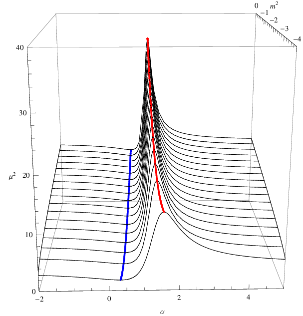

The profiles of functions are given in the left panel of Fig.3. The blue line is corresponding to the most stable mode of the solution while the red line is the second stable mode. On the right panel of Fig.3 we show the critical chemical potential as a function of , which is extracted from the left panel. The black dots are obtained from the shooting method in [20]. We can find that the values obtained from the two methods perfectly match each other with errors . This tiny error again indicates that the SL method can not only find the most stable mode, but also can find the second stable mode just like the shooting methods did in [20]. In addition, this tiny error also suggests that the trial function is very suitable to estimate the critical values of the phase transition. As a comparison, we also make use of the trial function to estimate the second stable mode. We find that in this case the errors between it and the shooting method is up to which is bigger than obtained from . Therefore, we find that only requiring the Dirichlet boundary condition of is not only viable for estimating the critical chemical potentials, but also makes the estimations more precise. The reason for the more precision is that for the Dirichlet boundary condition , the leading terms in the Taylor expansions of is rather than . In the next section, we give another exercise on p-wave insulator/superconductor phase transition in order to verify that the choice of is better than in estimating the critical values, if the boundary condition (3) is naturally satisfied by .
IV p-wave insulator/superconductor phase transition
Following the setup in [18], the p-wave insulator/superconductor phase transition can be studied by a SU(2) Einstein-Yang-Mills action with a negative cosmological constant. We will work in the probe limit, therefore we can only focus on the SU(2) Yang-Mills gauge field action, which is
| (28) |
in which is the Yang-Mills field strength, are the indices of the SU(2) Lie algebra generators, running from to . , where are the generators of the SU(2) Lie algebra with commutations . is a totally antisymmetric tensor with .
We will adopt the conventions in [18] to denote the line-element of AdS soliton as (We have set ),
| (29) |
where . We can choose the gauge field as
| (30) |
In this ansatz, the gauge boson is along -direction which will be charged under . In this case, is dual to a vector operator on the boundary field theory, while is corresponding to the chemical potential. Therefore, the non-vanishing of will spontaneously break the U(1)3 gauge symmetry, and then induce the superconducting phenomenon on the boundary.
From the above action, line-element and the ansatz of the fields, the EoMs of and are readily obtained as
| (31) | |||||
| (32) |
The asymptotic expansions of and near are
| (33) | |||||
| (34) |
where, from the dictionary of AdS/CFT correspondence, and are respectively the source and the expectation values of the dual operator , while and can be interpreted of the chemical potential and charge density of the dual field theory, respectively. There is also a trivial solution of the above EoMs, which is . In this case, the solution of is
| (35) |
In order for the regularity of at the tip , one has to impose , i.e., . Therefore, like what we did in the above section, we will set and just consider the EoM of near the critical point of the phase transition. For convenience, we will work in coordinate. Thus the EoM of Eq.(31) becomes
| (36) |
Again, introduce a trial function into the expansions of near as
| (37) |
The boundary condition sets . Then substituting Eq.(37) into Eq.(36), we reach
| (38) |
Multiply to both sides of the above equation, the EoM becomes
| (39) |
where
| (40) |
Considering that will naturally render the boundary condition(3) satisfied, i.e.,
| (41) |
we need not impose any restrictions on . Therefore, we simply assume that to satisfy , then the eigenvalues of can be obtained from the extremal values of the following functional
| (42) |

In Fig.4, we plot the profile of as a function of . The blue point is corresponding the most stable mode to the solution, while the red point is corresponding to the second stable mode. It is easy to get that , when ; , when . These two critical chemical potentials are in good agreement with the critical values in [20], in which for the first two lowest lying modes from the shooting method. We can see that the errors between the two methods are within . We also used the trial function to estimate the critical chemical potential as a comparison, in which the errors are up to which is bigger than . We again show that the SL method is suitable to estimate not only the most stable mode but also the second stable mode, moreover, the results obtained from the trial function is more precise than those from in previous literature [18].
V Conclusions and Discussions
In this paper, we took advantage of the analytical SL method to study the holographic insulator/superconductor phase transitions both for s-wave and p-wave, in the probe limit. We found that this analytical method could not only estimate the most stable (vacuum) mode, but also it could estimate the second stable mode. The results obtained from the SL method were perfectly in agreement with the numerical methods, such as the shooting method or the QNM method. 11 1 Actually from [20] we know that the QNMs are actually the eigenvalues of the system. Besides, SL method is also an approach to calculate the eigenvalues. Therefore, theoretically there is a one-to-one corresponding relation between the eigenvalues from the SL method and from the QNM method, although in our draft we could just calculate up to the second lowest eigenvalue by introducing a trial function for estimation. Besides, we argued that actually one could relax the boundary conditions of the trial function , depending on whether the boundary condition satisfied or not. If this boundary condition is automatically fulfilled by , we should only impose the Dirichlet boundary condition of without the Neumann boundary conditions. We made use of two examples to verify that only imposing Dirichlet boundary condition of the trial function would be more precise than additionally imposing another Neumann boundary condition. We believe that this kind of SL method can be readily extended to study the holographic superconductor/metal phase transition in black hole geometry.
The problem of this analytical SL methods is that it could hardly find the third stable mode of the solution, like the shooting method and QNM method did in previous papers [20]. This is because the SL method states that the eigenvalues are countably infinite and have a sequence like . Therefore, the third stable mode should have a critical value which is greater than the first two modes and . But from the profiles of or , the denominator and the numerator of the Rayleigh Quotient are greater than zero,22 2 Because in the Rayleigh Quotient (2), for , therefore, for . Therefore, the denominator of the Rayleigh Quotient is always positive. This argument goes the same way to the numerator of it. therefore, is positive and analytical in (please consult Fig.4). So the next extremal value of should be smaller than (the red point) because the function of is a continuous and smooth function of . This contradicts with the assertion in SL method that . Therefore, the analytical SL method for introducing a trial function depending on one parameter, such as , can only be applied to estimate the most and second stable mode of the solution. For higher modes, maybe one should introduce other types of the trial function depending on various parameters, or one should directly appeal to the shooting method or QNM method.
Acknowledgement
H.F.L. would like to thank Prof.Rong-Gen Cai and Dr.Hai-Qing Zhang for their indispensable discussions and comments. This work was supported by the Young Scientists Fund of the National Natural Science Foundation of China (Grant No.11205097), in part by the National Natural Science Foundation of China (Grant Nos. 11075098, 11175109), Supported by Program for the Innovative Talents of Higher Learning Institutions of Shanxi, and the Natural Science Foundation for Young Scientists of Shanxi Province,China (Grant No.2012021003-4) and by the Shanxi Datong University doctoral Sustentation Fund(No. 2011-B-04), China.
References
- [1] J. M. Maldacena, “The large N limit of superconformal field theories and supergravity,” Adv. Theor. Math. Phys. 2, 231 (1998) [Int. J. Theor. Phys. 38, 1113 (1999)] [arXiv:hep-th/9711200].
- [2] S. S. Gubser, I. R. Klebanov and A. M. Polyakov, “Gauge theory correlators from non-critical string theory,” Phys. Lett. B 428, 105 (1998) [arXiv:hep-th/9802109].
- [3] E. Witten, “Anti-de Sitter space and holography,” Adv. Theor. Math. Phys. 2, 253 (1998) [arXiv:hep-th/9802150].
- [4] E. Witten, “Anti-de Sitter space, thermal phase transition, and confinement in gauge theories,” Adv. Theor. Math. Phys. 2, 505 (1998) [hep-th/9803131].
- [5] D. T. Son, “Toward an AdS/cold atoms correspondence: A Geometric realization of the Schrodinger symmetry,” Phys. Rev. D 78, 046003 (2008) [arXiv:0804.3972 [hep-th]].
- [6] S. A. Hartnoll, C. P. Herzog and G. T. Horowitz, “Building a Holographic Superconductor,” Phys. Rev. Lett. 101, 031601 (2008) [arXiv:0803.3295 [hep-th]].
- [7] S. -S. Lee, “A Non-Fermi Liquid from a Charged Black Hole: A Critical Fermi Ball,” Phys. Rev. D 79, 086006 (2009) [arXiv:0809.3402 [hep-th]]
- [8] H. Liu, J. McGreevy and D. Vegh, “Non-Fermi liquids from holography,” Phys. Rev. D 83, 065029 (2011) [arXiv:0903.2477 [hep-th]]
- [9] M. Cubrovic, J. Zaanen and K. Schalm, “String Theory, Quantum Phase Transitions and the Emergent Fermi-Liquid,” Science 325, 439 (2009) [arXiv:0904.1993 [hep-th]].
- [10] T. Nishioka, S. Ryu and T. Takayanagi, “Holographic Superconductor/Insulator Transition at Zero Temperature,” JHEP 1003, 131 (2010) [arXiv:0911.0962 [hep-th]].
- [11] M. Montull, O. Pujol‘as, A. Salvioa, and P. J. Silva, ”Flux Periodicities and Quantum Hair on Holographic Superconductors,” Phys. Rev. lett. 107, 181601 2011
- [12] D. Roychowdhury ”Holographic droplets in p-wave insulator/superconductor transition,” JHEP 1305, 162 (2013) [arXiv:1304.6171 [hep-th].
- [13] M. Montull, O. Pujol‘as, A. Salvioa, and P. J. Silva, ”Magnetic Response in the Holographic Insulator/Superconductor Transition” JHEP 1204, 135 (2012) [arXiv:1102.0006 [hep-th].
- [14] G. T. Horowitz and R. C. Myers, “The AdS / CFT correspondence and a new positive energy conjecture for general relativity,” Phys. Rev. D 59, 026005 (1998) [hep-th/9808079].
- [15] G. Siopsis and J. Therrien, “Analytic Calculation of Properties of Holographic Superconductors,” JHEP 1005, 013 (2010) [arXiv:1003.4275 [hep-th]].
- [16] H. -B. Zeng, X. Gao, Y. Jiang and H. -S. Zong, “Analytical Computation of Critical Exponents in Several Holographic Superconductors,” JHEP 1105, 002 (2011) [arXiv:1012.5564 [hep-th]].
- [17] H. -F. Li, R. -G. Cai and H. -Q. Zhang, “Analytical Studies on Holographic Superconductors in Gauss-Bonnet Gravity,” JHEP 1104, 028 (2011) [arXiv:1103.2833 [hep-th]].
- [18] R. -G. Cai, H. -F. Li and H. -Q. Zhang, “Analytical Studies on Holographic Insulator/Superconductor Phase Transitions,” Phys. Rev. D 83, 126007 (2011) [arXiv:1103.5568 [hep-th]].
- [19] R. -G. Cai, L. Li, H. -Q. Zhang and Y. -L. Zhang, “Magnetic Field Effect on the Phase Transition in AdS Soliton Spacetime,” Phys. Rev. D 84, 126008 (2011) [arXiv:1109.5885 [hep-th]].
- [20] R. -G. Cai, X. He, H. -F. Li and H. -Q. Zhang, “Phase transitions in AdS soliton spacetime through marginally stable modes,” Phys. Rev. D 84, 046001 (2011) [arXiv:1105.5000 [hep-th]].
- [21] D. Momeni, M. R. Setare, ”A note on holographic superconductors with Weyl Corrections,” Mod. Phys. Lett. A 26, 2889 (2011) [arXiv:1106.0431 [hep-th]].
- [22] D. Momeni, N. Majd, and R. Myrzakulov ”p-wave holographic superconductors with Weyl corrections” EPL, 97, 61001 (2012) [arXiv:1204.1246 [hep-th]].
- [23] R. Courant and D. Hilbert, Methods of Mathematical Physics, Vol. 1, (1989) John Wiley & Sons.
- [24] Y. -Q. Wang, Y. -X. Liu, R. -G. Cai, S. Takeuchi and H. -Q. Zhang, “Holographic SIS Josephson Junction,” JHEP 1209, 058 (2012) [arXiv:1205.4406 [hep-th]].
- [25] I. R. Klebanov and E. Witten, “AdS / CFT correspondence and symmetry breaking,” Nucl. Phys. B 556, 89 (1999) [hep-th/9905104].