arXiv:1306.2895[hep-ex]
SLAC-PUB-15524
BABAR-PUB-13/003
Production of charged pions, kaons and protons in annihilations into hadrons at
Abstract
Inclusive production cross sections of , and per hadronic annihilation event are measured at a center-of-mass energy of 10.54 , using a relatively small sample of very high quality data from the BABAR experiment at the PEP-II -factory at the SLAC National Accelerator Laboratory. The drift chamber and Cherenkov detector provide clean samples of identified , , and over a wide range of momenta. Since the center-of-mass energy is below the threshold to produce a pair, with a bottom-quark meson, these data represent a pure sample with four quark flavors, and are used to test QCD predictions and hadronization models. Combined with measurements at other energies, in particular at the resonance, they also provide precise constraints on the scaling properties of the hadronization process over a wide energy range.
pacs
13.66.Bc, 13.87.Fh, 12.38.QkI Introduction
The production of hadrons from energetic quarks and gluons in high-energy collisions is well described by qualitative models, but there are few quantitative theoretical predictions. Detailed experimental information about hadron production allows the confining property of the strong interaction to be probed. An empirical understanding of confinement is important to the interpretation of much current and future high-energy data, in which the observable products of interactions and decays of heavy particles, known and yet to be discovered, appear as jets of hadrons. Measurements involving identified hadrons probe the influence on this process of hadron masses and quantum numbers such as strangeness, baryon number, and spin.
The process is understood to proceed through three stages. First, the quark () and antiquark () “fragment” via the radiation of gluons (), each of which can radiate further gluons or split into a pair. This process is, in principle, calculable in perturbative quantum chromodynamics (QCD), and there are calculations for up to four final-state partons, corresponding to second order in the strong coupling [1], where by “parton” we mean either a quark or a gluon. In addition, leading-order calculations exist for as many as six partons [2], as well as calculations to all orders in in the modified leading logarithm approximation (MLLA) [3]. There are also “parton shower” Monte Carlo simulations [4] that include an arbitrary number of , and branchings, with probabilities determined up to next-to-leading logarithm level.
In the second stage, these partons “hadronize”, or transform into “primary” hadrons, a step that is not understood quantitatively. The ansatz of local parton-hadron duality (LPHD) [3], that inclusive distributions of primary hadrons are the same up to a scale factor as those for partons, allows MLLA QCD to predict properties of distributions of the dimensionless variable for different hadrons. Here, is the scaled momentum, and and are the hadron momentum and the energy, respectively, in the center-of-mass (CM) frame. Predictions include the shape of the distribution and its dependence on hadron mass and . At sufficiently high , perturbative QCD has also been used to calculate the dependence of the distributions [5].
In the third stage, unstable primary hadrons decay into more stable particles, which can reach detector elements. Although proper lifetimes and decay branching fractions have been measured for many hadron species, these decays complicate fundamental measurements because many of the stable particles are decay products rather than primary hadrons. Previous measurements at colliders [6] indicate that decays of vector mesons, strange baryons, and decuplet baryons produce roughly two thirds of the stable particles; scalar and tensor mesons and radially excited baryons have also been observed and contribute additional secondary hadrons. Ideally one would measure every hadron species and distinguish primary hadrons from decay products on a statistical basis. A body of knowledge could be assembled by reconstructing increasingly heavy states and subtracting their known decay products from the measured rates of lighter hadrons. The measurement of the stable charged hadrons constitutes a first step in such a program.
There are several phenomenological models of hadronic jet production. To model the parton production stage, the HERWIG 5.8 [7], JETSET 7.4 [8] and UCLA 4.1 [9] event generators rely on combinations of first-order matrix elements and parton-shower simulations. For the hadronization stage, the HERWIG model splits the gluons produced in the first stage into pairs, combines these quarks and antiquarks locally to form colorless “clusters”, and decays the clusters into primary hadrons. The JETSET model represents the color field between the partons by a “string”, and breaks the string according to an iterative algorithm into several pieces, each corresponding to a primary hadron. The UCLA model generates whole events according to weights derived from phase space and Clebsch-Gordan coefficients. Each model contains free parameters controlling various aspects of the hadronization process, whose values have been tuned to reproduce data from annihilations. With a large number of parameters, JETSET has the potential to model many hadron species in detail, whereas UCLA and HERWIG seek a more global description with fewer parameters, including only one or two that control the relative rates of different species.
The scaling properties, or dependences, of hadron production are of particular interest. Since the process is governed by QCD, it is expected to be scale invariant, i.e. distributions of should be independent of except for the effects of hadron masses/phase space and the running of . The quark flavor composition varies with , and may also have substantial effects. Mass effects are observed to be large unless , where is the mass of the hadron in question, although current experimental precision is limited at lower energies. At high , the expected scaling violations have been calculated [5] and found to be consistent with available data, but experimental precision is limited for specific hadron species. The scaling violation for inclusive charged tracks has been used to extract under a number of assumptions about the dependence on event flavor and particle type [10]. Improved precision at 10.54 would provide stringent tests of such assumptions and more robust measurements of .
The production of the charged hadrons , , and has been studied in annihilations at values of 10 [11], 29 [12], 34 and 44 [13], 58 [14], 91 [15, 16, 17, 18], and at several points in the range 130–200 [19]. Recently, Belle has measured and production at 10.52 [20]. Results for 91 , near the pole, include precise measurements in inclusive hadronic events, as well as measurements for separated quark flavors, quark and gluon jets, and leading particles [21, 22]. The higher- and lower-energy measurements are, however, limited in precision and coverage. Improved precision over the full range at 10.54 would probe the large scaling violations in detail and provide sensitive new tests of QCD calculations and hadronization models.
In this article, we present measurements of the inclusive normalized production cross sections of charged pions, kaons, and protons per event. We use 0.91 of data recorded by the BABAR detector at the PEP-II storage ring at SLAC in March, 2002, at a CM energy of 10.54 . This is a small fraction of the BABAR “off-resonance” data, recorded during a period dedicated to the delivery of stable beams and constant luminosity. The detector experienced relatively low backgrounds and ran in its most efficient configuration, which was not changed in this period. In parallel, we analyze 3.6 of data recorded at the resonance (10.58 ) during the remainder of this period, February–April, 2002. This “on-resonance” sample provides independent, stringent systematic checks, and the combined samples provide data-derived calibrations of the tracking and particle identification performance. The uncertainties on the results are dominated by systematic contributions.
The detector and event selection are described in sections II–III. The selection of high quality charged tracks and their identification as pions, kaons or protons is discussed in section IV. The measurement of the cross sections, including corrections for the effects of backgrounds, detector efficiency and resolution, and the boost of the system in the BABAR laboratory frame, are described in section V. The results are compared with previous results and with the predictions of QCD and hadronization models in section VI, and are summarized in section VII.
II The BABAR Detector
The system is boosted in the BABAR laboratory frame by along the beam direction. We call this direction “forward”, , and denote quantities in the CM frame with an asterisk, and those in the laboratory frame with a subscript ‘lab’. For example, denotes the magnitude of a particle’s momentum in the CM frame and its angle with respect to the beam direction, and and denote the corresponding quantities in the laboratory frame. For events at , the maximum value is , but the maximum value depends on polar angle, with values of 3.8 at and 7 at 0.9. Thus, particles with a given value have different values in different regions of the detector, and are measured with different efficiencies and systematic uncertainties.
The BABAR detector is described in detail in Ref. [23]. In this analysis, we use charged tracks measured in the silicon vertex tracker (SVT) and the drift chamber (DCH), and identified in the DCH and the detector of internally reflected Cherenkov light (DIRC). We also use energy deposits measured in the CsI(Tl) crystal calorimeter (EMC) to identify electron tracks and construct quantities used in the event selection. These subdetectors operate in a 1.5 T solenoidal magnetic field.
The SVT comprises five double-sided layers of strip detectors, each of which measures a coordinate along () and azimuthally around () the beam axis. The DCH includes 40 layers of axial and stereo wires. Their combined resolution is , where is the momentum transverse to the beam axis. The DCH measures ionization energy loss () with a resolution of 8%.
The DIRC [24] consists of 144 fused silica radiator bars that guide Cherenkov photons to an expansion volume filled with water and equipped with 10,752 photomultiplier tubes. It covers the polar angle range . The refractive index of 1.473 corresponds to Cherenkov thresholds of 0.13, 0.48 and 0.87 for , and , respectively. The Cherenkov angles of detected photons are measured with an average resolution of 10.2 . Tracks with very high yield an average of 20 detected photons at , rising to 65 photons at the most forward and backward angles.
The EMC comprises 5,760 CsI(Tl) crystals in a projective geometry that measure clusters of energy with a resolution of , An algorithm identifies electrons using track momentum combined with EMC measurements of energy and shower shape. It has better than 95% efficiency for , and hadron misidentification rates of up to 1% for and at most 0.1% for higher momenta.
III Hadronic Event Selection
The event selection is optimized for low bias across the hadron momentum spectra and event multiplicity distribution, while minimizing backgrounds from other physics processes and beam-wall and beam-gas interactions. After fitting each combination of three or more reconstructed charged tracks to a common vertex, we require:
- 1.
at least three charged tracks and one good vertex, where a good vertex has a confidence level above 0.01;
- 2.
the good vertex with the highest track multiplicity to lie within 5 of the beam axis, and within 5 of the center of the collision region in ;
- 3.
the second Fox-Wolfram moment [25] to be less than 0.9;
- 4.
the sum of the energies of the charged tracks and unassociated neutral clusters to be in the range 5–14 ;
- 5.
the polar angle of the event thrust [26] axis in the CM frame to satisfy ;
- 6.
the track with the highest not to be identified as an electron in events with fewer than six tracks, and neither of the two highest- tracks to be identified as an electron in events with only three tracks.
Criteria 3 and 6 reject leptonic events, , , and . Criteria 4 and 5 ensure that the event is well contained within the sensitive volume of the detector, resulting in smaller corrections and lower biases. These criteria select 2.2 million events in our off-resonance signal sample and 11.8 million events in our on-resonance calibration sample. About 27% of the events in the latter sample are decays.
We evaluate the performance of the event selection using the data and a number of simulations, each consisting of a generator for a certain type of event combined with a detailed simulation of the BABAR detector using the GEANT4 [27] package. For signal events, we use the JETSET [8] event generator and obtain simulated selection efficiencies of 0.68 for , and events, and 0.73 for events. As cross checks, we also use the UCLA model combined with GEANT4, and the JETSET, UCLA and HERWIG models with a fast detector simulation and several different parameter sets. These give efficiency variations of at most 0.5%. In all cases, the largest signal loss is due to the requirement on , which ensures that the event is well contained within the sensitive volume of the detector, resulting in low and multiplicity biases. We find consistency between data and simulation in a number of distributions of event and track quantities; the largest discrepancy we observe is a possible shift in the distribution (see Fig. 1), which could indicate an efficiency difference of at most 0.5%.
We use the KORALB [28] generator to simulate - and -pair events. The former provide a negligible contribution, but the latter are the largest source of background, estimated to be 4.5% of the selected events and to contribute up to 25% of the charged tracks at the highest momenta. However, the relevant properties of -pair events are well measured [29], and their contributions can be simulated and subtracted reliably.
Radiative Bhabha events () are an especially problematic background, as their cross section in the very forward and backward regions is larger than the cross section and varies rapidly with . Bremsstrahlung, photon conversions, and other interactions in the detector material are difficult to simulate in these regions, and can result in events with 3–6 tracks, most of which are from electrons or positrons. Simulations using the BHWIDE [30] generator predict that these events are reduced to a negligible level by criteria 1–5 plus a requirement that the highest- track in the 3- and 4-track events not be identified as an electron. However, a comparison of and angular distributions in the selected data indicates a larger contribution. Therefore, we impose the tighter vetoes given in criterion 6, and estimate from the data a residual radiative Bhabha event contribution of 0.1% of the selected events and up to 8% of the charged tracks at our highest momenta and values.
Initial-state radiation (ISR), , produces hadronic events with a lower effective CM energy. Low-energy ISR photons are present in all events and are simulated adequately in the JETSET model. The event selection is designed to suppress events with higher-energy ISR photons, including radiative return to the , and resonances (whose decays have very different inclusive properties from events) and events with a very energetic ISR photon recoiling against a hadronic system, which can mimic 2-jet events. Using the AFKQED generator [31], we find that the combination of the requirements on and reduces the energetic-ISR background to negligible levels, and the background to one event in .

We use the GAMGAM [32] generator to study backgrounds from 2-photon () processes, hadrons. Neither the total cross section nor those for any specific final states are known, but such events have relatively low track multiplicity and since the final-state and some of the hadrons generally go undetected along the beam direction. The distribution for events in the data satisfying all other selection criteria is shown in Fig. 1. It features a structure in the 1-5 range that is not described by the signal plus -pair simulations, but can be described qualitatively by the addition of events. Since the mixture of final states is unknown, we consider , which has the largest fraction of events with 5 of any final state with at least three tracks. The simulated distribution is shown as the shaded histogram in Fig. 1. If normalized to account for the entire excess in the data, such events would make up less than 1% of the selected sample (5 14 ), with a track momentum distribution similar to that in -pair events. We take this as an upper limit on our background and vary its contribution over a wide range in evaluating the systematic uncertainty, as discussed in Sec. V.2.
Backgrounds from beam-gas and beam-wall interactions can be studied using distributions of event vertex position in the data. From the distribution in distance from the beam axis for events satisfying all selection criteria except those on the vertex position, we conclude that the beam-wall background is negligible. From the distribution in after including the requirement that the vertex be within 5 mm of the beam axis, we estimate that four beam-gas events are selected per signal events. We neglect both of these backgrounds.
We consider a number of other possible backgrounds, including two-photon events with one or both detected and other higher-order quantum electrodynamics (QED) processes producing four charged leptons or two leptons and a pair; all are found to be negligible. We estimate that the selected sample is 95.41.1% pure in events, with the background dominated by -pairs and the uncertainty by events. The on-resonance calibration sample contains the same mixture of and background events, plus a 27% contribution from decays.
IV Charged Track Selection and Identification
The identification of charged tracks as pions, kaons or protons is performed using an algorithm that combines the momentum and ionization energy loss measured in the DCH and the velocity measured via the Cherenkov angle in the DIRC. To ensure reliable measurements of these quantities, we require tracks to have: i) at least 20 measured coordinates in the DCH; ii) at least 5 coordinates in the SVT, including at least 3 in ; iii) a distance of closest approach to the beam axis of less than 1 ; iv) a transverse momentum ; v) a polar angle satisfying ; and vi) an extrapolated trajectory that intersects a DIRC bar. The first criterion ensures good resolution, the first three criteria select tracks from particles that originate from the primary interaction and do not decay in flight or interact before reaching the DIRC, and the combination of all six criteria yields tracks well within the DIRC fiducial volume, with good momentum and polar angle resolution.
These criteria suppress tracks from decays of long-lived particles such as and hadrons, which are included in many previous measurements. Here, we report cross sections for two classes of tracks, denoted “prompt” and “conventional”. We first measure prompt hadrons, defined as primary hadrons or products of a decay chain in which all particles have lifetimes shorter than s. This includes products of all charmed hadron decays, as well as those of strongly or electromagnetically decaying strange particles, but not those of weakly decaying strange particles. We then obtain the conventional quantities by adding the decay daughters of particles with lifetimes in the range 1–310-11 s, i.e., and weakly decaying strange baryons. For this we use existing measurements of and strange baryon production [33, 34]. Either or both cross sections can be compared with other measurements, and used to test QCD and model predictions.
In selected simulated events, these criteria accept 82% of the prompt charged particles generated within the target range and with . This efficiency rises slowly from 80% at to 86% at the highest momentum, and is almost independent of particle type, polar angle, event flavor, and track multiplicity. Corrections to the simulation are discussed in Sec. V.3.
Since the system is boosted in the laboratory frame, we divide the selected tracks into six regions of : [0.78,0.33], [0.33,0.05], [0.05,0.36], [0.36,0.6], [0.6,0.77] and [0.77,0.88], denoted to , and analyze each region separately. These correspond to regions of roughly equal width in between 0.92 and 0.69. The tracks in each region arise from the same underlying distribution, but are boosted into different ranges of . Also, heavier particles are boosted to higher , with low- protons and kaons populating the forward regions preferentially. Thus we perform multiple (up to six) measurements for each value, each from a different range and in a different region of the detector. Their comparison provides a powerful set of cross checks on detector performance and material interactions, backgrounds, the true and distributions, and the boost value itself.
IV.1 Charged Hadron Identification
The measurement from the DCH provides very good separation between low- particles, i.e., between and ( and ) below about 0.5 (0.8) . There is also modest separation, of 1–3 standard deviations (), in the relativistic rise region above about 2 , and the separation varies rapidly at intermediate . For each accepted track, we calculate a set of five likelihoods , , each reflecting the degree of consistency of its measured value with hypothesis .
The Cherenkov angle measurement from the DIRC provides very good separation between particles with between the Cherenkov threshold and the resolution limit of about 4 for vs. and 6.5 for vs. . The number of expected photons varies rapidly with just above threshold, and the number detected for each track provides additional information. A track can be classified as being below threshold by counting the detected photons at the angles expected for each above-threshold particle type and comparing with the hypothesis that only background is present. To make full use of this information, we maximize a global likelihood for the set of reconstructed tracks in each event, which considers backgrounds, photons that could have been emitted by more than one track, and multiple angles from a given track. For each track, we calculate a set of five likelihoods , , assuming the best hypothesis for all other tracks. These provide - (-) separation that rises rapidly with from zero at the () Cherenkov threshold of 0.13 (0.48) , to a roughly constant value, from which it falls off above about 2.5 (4.5) .

To make use of both DCH and DIRC information, we consider the log-likelihood differences , where det DCH, DIRC, and we identify tracks by their positions in the vs. planes. The procedure is illustrated in Fig. 2 for simulated (lower left) and (upper right) with and . Here the DIRC provides clear separation for all but a few percent of the tracks (most of the entries at the left and right edges are overflows), but long tails are visible in the distributions for both and . The DCH separation is smaller, but the tails are shorter. To be identified as a , a track must lie below a line in the – plane (see Fig. 2) and below another line in the – plane. Similarly, an identified lies above a line (dashed in Fig. 2) in the – plane and below a line in the – plane, and an identified lies above lines in the – and – planes.
The parameters describing the lines vary smoothly with and , and are optimized [35] to keep the misidentification rates as low as reasonably possible, while maintaining high identification efficiencies that vary slowly with both and . The slopes are zero (i.e. only information is used) for below the lower of the two Cherenkov thresholds, begin to decrease slowly at that threshold, and become large and negative above about 2.5 ; although provides some separation in this region, the systematic uncertainties are minimized by using it only to reject outlying tracks. In some cases the two lines in a given plane are the same; in most cases they are nearly parallel and separated by a few units, and tracks in between are not identified as any hadron type. Fewer than 0.1% of the tracks are identified as more than one type, and these are reclassified as unidentified.
Electrons and muons represent only a small fraction of the tracks in hadronic events at (at most 2%), and their production is understood at the level of 10% or better (see Sec. V.5). They can be suppressed at this point using calorimeter and muon system information, and we have done this as a cross check, obtaining consistent results. However, this also rejects some signal tracks, and the total systematic uncertainties are minimized by including and in the pion category at this stage, and subtracting them later. We therefore define a sample. High-momentum and almost all are indistinguishable from in the DCH or DIRC, so are included by the criteria noted so far. The DIRC does separate from in a narrow range near 0.2 , but we use only information in this range. To accommodate low-momentum , we include tracks with below 2 that satisfy requirements in the – and – planes.
We quantify the performance of our hadron identification procedure in terms of a momentum-dependent identification efficiency matrix , where each element represents the probability that a selected track from a true -hadron is identified as a -hadron, with . The matrix predicted by the detector simulation for our most forward polar angle region, , which covers the widest range, is shown as the dashed lines in Fig. 3. The efficiencies for correct identification are predicted to be very high at low , where separation is good, then transition smoothly to a plateau where the Cherenkov angle provides good separation, then fall off at higher where the Cherenkov angles for different particles converge. The predicted probabilities for misidentifying a particle as a different type are below 2.5%. Essentially all tracks are identified as some particle type at low , 1–3% are classified as ambiguous in the plateau regions, and larger fractions are so classified as the efficiency falls off, since we choose to maintain constant or falling misidentification rates.
Similar performance is predicted in the other regions. In and , the two most backward regions, does not exceed 3.5–4 , so no fall off is visible in at high , and and drop only to 30–70% of their plateau values. Thus we are able to measure the high range well in multiple regions. In the next few subsections, however, we focus on , since it spans the widest range in efficiencies and requires the largest corrections to the simulation.

IV.2 Calibration of the Identification Efficiencies
We calibrate the efficiency matrix from the combined off- and on-resonance data set, using samples of tracks with known hadron content and characteristics as similar as possible to our selected tracks. For example, we construct candidates from tracks satisfying criteria (i) and (iv)–(vi) presented at the beginning of Sec. IV, with a less restrictive requirement of three coordinates in the SVT and an additional requirement that there be a coordinate from one of the two outer layers of the DCH. Pairs of oppositely charged tracks must have a fitted vertex more than 0.5 from the beam axis, a reconstructed total momentum direction within 50 mrad of the line between their fitted vertex and the event vertex, and an invariant mass in the range 486–506 . The percent-level non- contribution is predominantly from pions, so these tracks constitute a clean sample of that are produced in hadronic events and cross most of the tracking system. In simulated events, this sample has values within 0.5% of those of the prompt in the same events. We calculate efficiencies from this sample in both data and simulation, and use their differences to correct the prompt simulation. This sample covers up to about 1.5 with high precision.
A similar selection of and candidates provides a sample of 0.4–3.5 (and another sample of soft pions) in hadronic events. We also reconstruct two samples of decays in which either the or is identified, providing 0.2–2 and samples that are subsamples of our main sample. These samples contain substantial backgrounds, and we extract , , and from sets of simultaneous fits to the four or invariant mass distributions in which the or the other kaon is identified as a pion, kaon, proton or no type.
We obtain samples of 0.6–5 and by reconstructing candidate (and charge conjugate) decays and selecting those with a – mass difference in the range 143–148 . The invariant distribution shows a signal with a peak signal-to-background of eleven. These tracks are predominantly from decays and events, but have simulated and values within 1% and 0.5%, respectively, of those from all prompt and in hadronic events. Requiring the () candidate track to be so identified and the () track to satisfy our selection criteria, we evaluate () as the fraction of the sideband-subtracted entries in the peak in which the () is identified as type .
We select events in which one of the decays contains a single charged track (1-prong) and the other contains one or three (3-prong) charged tracks. These tracks constitute samples that are not from a hadronic jet environment and have different :: content, as well as a small but well known component. However, these samples have simulated identification efficiencies within a few percent of those for in hadronic events, and they allow us to study high- tracks and tracks that are isolated (1-prong) or relatively close together (3-prong) in the detector. We also apply independent electron and muon selectors to the 1-prong sample, in order to check that the small differences in performance between , and are simulated correctly.
Results from the different calibration samples are consistent where they overlap, as are those from positively and negatively charged tracks and from on- and off-resonance data. Considering the set of constraints provided by these samples, we derive corrections to the simulated elements that vary smoothly with and . The correction to each in each region is a continuous, piecewise-linear function of , with an uncertainty given by the statistically most precise calibration sample at each point. The resulting calibrated efficiencies in the region are shown as the gray/green bands in Fig. 3; their centers represent the calibrated efficiencies, and their half widths the uncertainties.
The pion efficiencies (left column of Fig. 3) are measured well over the full range, with corrections and uncertainties near or below the percent level for . There are substantial corrections to and in the 3–5 range, which is sensitive to the details of the DIRC geometry and backgrounds.
The kaon efficiencies (middle column of Fig. 3) are measured for with somewhat larger uncertainties than for . The corrections to and are similar at most to those on and , respectively, as expected from the near symmetry in the and Cherenkov angle measurements. They have opposite sign, as expected, in the region just above kaon threshold, 0.5–1 . The large correction to near 6 is consistent with the corrections to and with scaled by a factor of roughly 1.9, the ratio of the proton and kaon masses, as expected.
Below 0.4 , the kaon calibration samples have high backgrounds and do not yield useful results. However, the identification efficiencies are very high, we expect strong correlations between hadron types up to 0.6 , and the calibration data are consistent with full correlation between 0.4 and 0.6 . Therefore, we apply the same small corrections to as for , and to and as for at 0.2 , with the uncertainty doubled arbitrarily to account for any incomplete correlation. We apply the corrections and uncertainties from the kaon calibration samples to and at 0.6 , and vary the corrections and uncertainties linearly between 0.2 and 0.6 . Due to the higher proton mass, the corresponding region in extends to 1.0 , so we match the corrections at that value.
The proton efficiencies (right column of Fig. 3) are measured well in the range 0.8–3.5 , and the corrections show the expected correlations with the other elements. Again, we expect complete correlations at low , and we apply the same corrections to , , and as for , , and , respectively, at 0.2 , with doubled uncertainties. We then match them to their respective proton calibration values at 1 . Above 3.5 , the statistical precision of the proton calibration sample is limited, and we exploit the correlation expected between in the 2–6.5 range, and and in the corresponding 1.1–3.4 range. The three corrections are consistent in the lower part of this range, and in the upper part we average the corrections to and , scale them up in , and apply them to with an uncertainty twice that on the correction. We match to the proton calibration sample at 3.1 , where the uncertainties from the two approaches are comparable.
Due to the low value of the proton fraction, the criteria for proton identification are more stringent than for pion or kaon identification at high , so that and are smaller than the other misidentification rates, as are the corrections.
Corrections to the efficiencies in the other regions are similar in form and generally smaller than those shown in Fig. 3. Even though the uncertainties of some misidentification rates are relatively large, they result in small systematic uncertainties of the result, since the rates themselves are sufficiently low. The uncertainties of the correct identification efficiencies are important, especially at high . However, high- particles are measured well in the more backward regions, and the final result is an average over the six regions.
V Measurement of the Differential Cross Sections
The objects of this measurement are the production cross sections per unit , ), , normalized to the total hadronic event cross section at our CM energy of 10.54 . We present these in the equivalent and conventional form , where and are the numbers of hadronic events and -particles, respectively.
From our samples of identified , and , we use the corrected identification efficiency matrices described in the preceding section to construct the raw production rates , , defined as the numbers of reconstructed particles per selected event per unit momentum in the laboratory frame. We subtract backgrounds and apply corrections to account for the effects of detector efficiency and resolution, and the event selection procedure. We do this separately in each of the six regions, and also in the on-resonance sample for control purposes.
We transform each corrected rate into a cross section in the CM frame, where we compare and combine the results from the six regions. Subtracting the expected contributions from leptons, we obtain our prompt results, . We add the expected contributions from decays of and weakly decaying strange baryons to obtain conventional cross sections, and we calculate ratios of cross sections and charged hadron fractions. Each of these steps is described in detail in the following subsections, and each involves a number of systematic checks and uncertainties. The systematic uncertainties are summarized in the final subsection.
V.1 Cross Sections in the Laboratory Frame
In each bin, we count , the number of tracks identified as type . These can be related to the true fractions of tracks that are of type by , where is the total number of selected tracks and the efficiency matrix is described in Sec. IV. We first solve this set of equations in each bin for the three values, and check that their sum is consistent with unity. This check is sensitive to many systematic effects on , and if we apply no corrections to the simulated , we find significant differences from unity in several places, most notably in the DCH-DIRC crossover region near 0.7 and at the highest momenta in the forward polar angle regions. The on-resonance control sample shows the same differences. After the corrections, the sum is consistent with unity in all bins within the systematic uncertainties obtained by propagating the uncertainties on the nine . The fractions and their sum in the most forward region, , are shown in Fig. 4. Neighboring points are correlated due to the efficiency correction procedure.

We then recalculate the fractions with the added constraint that their sum be unity. The recalculated fractions are also shown in Fig. 4, and are almost indistinguishable from the unconstrained fractions. In the systematic error propagation, we account for the constraint by varying the three efficiencies independently, and in each case varying both corresponding misidentification rates in the opposite direction. Both the statistical and systematic uncertainties decrease slightly with the addition of the constraint. It also introduces strong statistical correlations between the three particle types, but since the results are dominated by systematic effects, we neglect these.
Several additional systematic checks are performed, including varying the misidentification rates by three times their uncertainties, changing the ranges over which we fit the corrections to , using different event flavor mixtures in the simulation, and using the efficiencies measured in the control samples directly, rather than using them to correct the simulation. We find no change in the results larger than the relevant systematic uncertainty.
Each fraction is multiplied by the number of accepted tracks in that bin and divided by the number of selected hadronic events and by the bin width to obtain raw normalized cross sections.
V.2 Background Subtraction
We subtract backgrounds due to other physics processes, interactions in the detector material, and strange-particle decay products. As discussed in Sec. III, there are three physics processes with non-negligible background contributions to our event sample: -pair, two-photon and radiative Bhabha events. Figure 5 shows the simulated fractional contributions to the selected tracks in region from these three sources.
The contribution from -pair events is small at low , but grows steadily to over 20% at higher momenta. There are similar contributions in the other regions. The simulation of -pair production and decay is reliable at the sub-percent level, and our detector simulation is reliable (after the corrections described in Sec. V.3) to 1–2%. However, since we normalize per selected event, we must consider the relative event selection efficiency. Here, our simulation is also quite reliable for -pairs, but less so for hadronic events, discussed in Sec. V.6, and the uncertainty corresponds to a roughly constant 10% relative uncertainty on the tracks from -pair events. We therefore subtract the absolute prediction of the simulation with a 10% relative uncertainty.

The contribution from two-photon events is not well understood, but we can set an upper limit by scaling our simulated sample to account for the structure observed at low , discussed in Sec. III and shown in Fig. 1. The resulting contribution is shown by the triangles in Fig. 5. Due to the kinematics of events and the detector acceptance, this background is highest in , somewhat smaller in , and about half as large in the central regions. Most events contain more charged and neutral hadrons than the final state, some of which are outside the acceptance, yielding smaller values of . Therefore, we expect to select far fewer events than indicated by this sample, containing mostly lower- tracks, and Fig. 5 shows a substantial overestimate at high and an upper bound at lower . This limit is at most 4% and well below the -pair contribution, so we make no correction, but assign a systematic uncertainty corresponding to one half of the limit in each bin.
As discussed in Sec. III, the simulation predicts a negligible contribution from radiative Bhabha events, but may be unreliable, especially in the forward and backward directions. Due to the -channel contribution to their production process, such events would exhibit a charge asymmetry with a characteristic dependence on and . In our selected sample, we observe significant differences between positively and negatively charged tracks that reach 10% and 4% at the highest in the most backward and forward regions, respectively, and show an angular dependence consistent with radiative Bhabha events. We make a smooth parametrization of this difference, and subtract it from our cross section. The effect is a few percent at high momenta in the forward (see Fig. 5) and backward regions, but below 1% in the central regions. This procedure also accounts for any residual events from or other higher-order QED processes with forward-peaking cross sections.
After subtracting these -pair and radiative Bhabha backgrounds, we normalize by the estimated number of hadronic events in the selected sample, to obtain background-subtracted differential cross sections.
Interactions of particles with the detector material can lead to tracking inefficiencies, which are discussed in Sec. V.3, and also to the production of extraneous charged tracks that satisfy the signal-track criteria. Most interaction products fail the selection criteria, but two categories require care: a highly asymmetric photon conversion can produce an electron or positron that points back to the event vertex; and a pion interacting with a nucleon through a resonance can produce a proton nearly collinear with the pion. Figure 6 shows the simulated fractional contributions from interaction products. Photon conversions account for the vast majority, as much as 1.5% of the selected tracks at the lowest value, but well below 1% over most of the range. We have measured the photon conversion rate in our data, and the simulated rate lies within 20% of this rate for all , so we subtract the simulated fractional contribution to the sample, shown in the right plot of Fig. 6. Since the measurement uses conversions with two tracks that fail our selection criteria, and the chance of passing depends on details of the detector simulation, we assign an arbitrary and conservative systematic uncertainty equal to 50% of the correction.

Protons produced in the detector material represent a small fraction of all selected tracks, but as much as 4% and 15% of those identified as protons in the lowest kinematically allowed bins in (shown in Fig. 6) and , respectively. There is a concentration of material in the BABAR detector between the SVT and the DCH, and protons produced in this region can be studied using tracks that are identified by our algorithm as protons, but have measured in the SVT inconsistent with a proton and consistent with a pion. Our study revealed a problem with the simulation of the resonances in our version of GEANT, for which we apply a correction. We subtract the corrected simulated contributions of such protons and apply a uniform 50% relative uncertainty, which is slightly larger than the statistical uncertainty on the study in each region.
Very few antiprotons are produced in material interactions, but they suffer from similar uncertainties in the loss rate (see Sec. V.3). We measure and cross sections separately, and the results are consistent within these systematic uncertainties. The simulation predicts a very small number of kaons from detector interactions, and we subtract the predicted fraction with an arbitrary 50% uncertainty. The simulation also includes tracks arising from beam-related backgrounds and noise in the detector, by overlaying untriggered events from beam crossings close in time to triggered events. These are a small fraction of the tracks in Fig. 6, and are included in the correction.
There are also residual tracks in the sample from weak decays of strange particles that we must exclude from our prompt sample. We evaluate these by reweighting our simulated and spectra to reproduce the average of the measured spectra at or near our CM energy [33, 34], reweighting our simulated spectrum to match the measured spectrum [33, 34], and applying the same weights to our simulated baryon spectra. The weighted simulation predicts that at the lowest , about 2% of the selected tracks are from decays and a further 3% from strange baryon decays, with both contributions falling rapidly as increases. About 13% of the selected tracks in the lower half of the range are from strange baryon decays, and this falls slowly toward 4% at the highest . There are also smaller contributions of from , and decays, and from decays.
We subtract the simulated fractions of these tracks from each cross section, and assign systematic uncertainties to the and strange baryon contributions based on the uncertainties on the corresponding measured spectra [33, 34]. The assigned uncertainties are parametrized with smooth functions that vary with between 5% and 35% over the bulk of distributions, and increase toward 100% at zero and the kinematic limits, where the contributions vanish. We assign an arbitrary 50% relative uncertainty to all other sources.
V.3 Track Selection Efficiency
Next, we correct the background-subtracted cross sections for the track and event selection efficiencies, to obtain corrected cross sections, per hadronic event, for each hadron type. Figure 7 shows these efficiencies for the three particle types as functions of in region .
The solid lines in Fig. 7 represent the simulated fractions of particles within this region that are in a selected event. They are well below unity here, since is near the edge of our acceptance, but peak near 95% in the central regions. Most of the dependence arises from the two-jet topology of events. Softer tracks are farther, on average, from the thrust axis, and their distribution becomes nearly isotropic at very low , where all three fractions approach the average event selection efficiency of 72%. The highest- tracks tend to define the thrust axis, and the fractions drop at high in and , which span our thrust axis requirement. The track multiplicity and electron veto criteria introduce smaller biases against high- tracks in all regions.

These biases depend on several aspects of the hadronization process, which is the object of this measurement. Since it is not understood in detail, especially in extreme cases such as events with one very high-momentum track, we compare a number of inclusive track momentum and polar angle distributions in the data and simulation. We find a number of inconsistencies, some of which are described in Sec. VI. We address these by reweighting the simulated distributions to match the data, and by comparing a number of different generators and parameter values without detector simulation. We find changes in the event selection bias that are much smaller than the other uncertainties.
The dashed lines in Fig. 7 represent the simulated efficiencies for a particle in a selected event to produce a selected track. They are zero by definition for tracks with below 0.2 . The efficiency rises rapidly to 80% at 1 , then increases slowly to an asymptotic value of about 85%. The kaon and proton efficiencies rise more slowly due to decays in flight and interactions in the detector material, respectively, then show behavior similar to the pions. This strong similarity is present for prompt particles, but the pion and proton efficiencies would decrease by up to 10% if and strange baryon decay products were included. These efficiencies vary little with polar angle.
We perform a number of studies to check and correct the simulated efficiencies [36]. A study of high quality tracks reconstructed in the SVT alone and extrapolated into the DCH gives information on both the intrinsic efficiency of the DCH and losses in the material between them. The simulation is found to be consistent with the data at high , but corrections of up to 3% are needed at lower . A similar study uses pairs of DCH tracks that form a or candidate with a reconstructed vertex inconsistent with the event vertex but within the innermost layer of the SVT. This gives information on the SVT efficiency, indicating the need for 1-3% corrections at low and 0.5% corrections overall. A further study [37] of identified tracks with a kink (which revealed the problem in GEANT4 noted in Sec. V.2) provides a check of the simulation of decays in flight, and indicates different material interaction corrections for pions, kaons and protons.
We also compare the fraction of tracks in the data and simulation that satisfy each of the selection criteria after all combinations of the other criteria have been applied. An overall difference could arise from a deficiency in either the physics or the detector simulation, so is of limited use. However, by studying differences as a function of identified track type, charge and polar angle, a number of potential problems with the detector simulation can be corrected or limited. We find consistency overall, but we confirm the discrepancies found in the studies just described, and also identify a problem with the simulation of the DCH hit thresholds that affects particles with small . The effect is small except at values near the minimum of the curve in the most central region, where it is as large as 1.3%.
Combining this information, we derive a set of corrections to the simulated efficiencies. These are shown as bands in Fig. 7, where the half-widths indicate the total uncertainties. The corrections are below 1% with uncertainties of 0.8% for . At lower momenta, the correction to the kaon efficiency is at the percent level, but the pion (proton) efficiency is reduced (increased) by as much as 6.5% (9%) with uncertainties of up to one-third of the correction. The corrections have the same form in the other regions, but are smaller in proportion to the amount of material traversed.
The simulated interaction rates are different for positively and negatively charged particles, as are some of the corrections. We perform the analysis separately for the two charges up to this point, and compare their cross sections at each stage in each region. Without the efficiency correction, we observe differences consistent with expectations. The fully corrected cross sections are consistent with each other within the relevant systematic uncertainties.
V.4 Cross Sections in the CM Frame
At this point we have cross sections for hadrons produced in six regions as functions of their measured . The measured value can differ from the true value because of finite momentum resolution, and low- particles can suffer energy loss before the DCH that reduces the measured . These are both small effects on this measurement, and it is convenient to include corrections for them in the transformation to the CM frame, discussed in this section. We verify the quality of our simulation by comparing the masses and widths of the , , and signals with those measured in the data (see Ref. [38]). The small differences have negligible effects on this measurement, and we assign no systematic uncertainty from this source.
Differential cross sections in the laboratory frame can, in principle, be transformed into the CM frame in a model-independent way. However, large nonlinearities for low- and particles make this challenging, and we choose instead a method that is explicitly model dependent, but allows us to check the simulation at each stage and evaluate systematic uncertainties reliably.
For each particle type and each region, we first calculate production fractions and an inverse migration matrix from the simulation, where: is the fraction of particles produced in the bin that are boosted into this region; and is the fraction of those boosted into the bin that arise from the bin. The transformation can then be written as
| (1) |
The widths of the regions are such that 4–5 bins contribute to each bin at most momenta. At low , this increases to as many as 9 bins for 0.3 protons in .
The matrix is sensitive to the shape of the true distribution, and the transformation is incorrect if that is not modeled well. The effect is small (zero) if the distribution varies smoothly (linearly) over the relevant range, but can be large near a peak or inflection point and at high where distributions fall exponentially. We use an iterative procedure in which we reweight the simulation to match the measured distribution, redo the transformation, and repeat until the changes are sufficiently small. This procedure is reliable if the initial differences are not too large. In each case we find a measured distribution with statistically significant differences in shape from the simulation, but the first iteration produces changes smaller than the statistical uncertainties, and changes from the second iteration are negligible. We assign no systematic uncertainty from this source.


is insensitive to the true distribution, whereas the are quite sensitive to but almost insensitive to the true distribution. The distribution must therefore be modeled sufficiently well. It has the approximate form with , where is small for low but approaches 1 for high . We compare the cross sections measured in the six regions, which are shown for the on-resonance data in Fig. 8 divided by their weighted average value (see below) in each bin. The uncertainties are statistical only, and are correlated with their 2–3 nearest neighbors as a result of the transformation to the CM frame. The solid (dashed) lines indicate (twice) the root-mean-square (RMS) variation expected from the systematic uncertainties discussed so far. The largest contribution to this is from the particle identification efficiencies, which are evaluated independently in each region, but are correlated over ranges of several bins. Below 0.5 , uncertainties of the tracking efficiency are also important; these are similar among regions for a given value, but vary at a given , and are correlated within each region.
Overall, the data are consistent within the expected variation, and the off-resonance data show a similar set of variations. An incorrectly simulated would be visible here as a specific pattern of differences between the at that , roughly parabolic in with (or the reverse). The amplitude of this pattern would be expected to vary slowly with over several bins, or perhaps across the full range. No such pattern is visible in Fig. 8, and we set limits on any mismodeling by fitting the expected pattern to the in each bin. For each particle we find the largest amplitude averaged over three neighboring bins. They correspond to 0.5%, 1% and 2% shifts in , or 1%, 2% and 4% spreads between the and points in Fig. 8, for pions, kaons and protons, respectively. We take these limiting shifts in as conservative systematic uncertainties in each region and at all . The corresponding shifts in the other are smaller, and those in , and are of opposite sign; we take this correlation into account in the average, leading to a partial cancellation.
This comparison also limits several other systematic effects. For example, it is sensitive to an incorrect boost value, which would give with the differences increasing linearly with ; the data limit any such effect to a negligible level. A poor simulation of material interactions or soft-track efficiencies would appear as a spread in the , with a particular ordering, as approaches its lowest value. We observe up to 6% spreads without the corrections described in Sec. V.3, but no significant spread is visible in Fig. 8. In the plot, the highest- points for – are low. This may be due to a systematic effect in the kaon identification efficiencies, but the uncertainties for these points are large and they contribute little to the average. We check for the characteristic ordering and dependence expected from residual mismodeling of the distribution, and we observe no significant effects.
In each bin, we average the values from the regions weighted by their total uncertainties. Due to the low identification efficiencies at high , some measurements have very large uncertainties, and we do not use the data above values of 5.00, 4.75, 4.50, and 4.25 in , , , and , respectively. The uncertainties are relatively large just below these cutoff points, so that the high- measurements are dominated by the backward regions where the momenta are boosted downward and identification efficiencies are high. Low- protons are boosted very far forward, and only contributes below 0.30 , with , , , , and starting at 0.30, 0.45, 0.60, 0.70, and 0.75 . Three (five) regions contribute to the lowest- kaon (pion) point, with the others coming in at 0.25, 0.35, and 0.45 (0.30 ). All six regions contribute over most of the range.
The particle-identification uncertainties in different regions are independent of each other, since they are derived from distinct control samples. These and the statistical uncertainties are therefore reduced according to the number of regions contributing to the average in each bin. The uncertainties due to the distributions are common to all regions, but are anticorrelated between the central and forward/backward regions, so they are also reduced accordingly. We take all other uncertainties to be completely correlated between the regions and average them, but the weighting takes advantage of the variations with and/or .
V.5 Cross Sections for Prompt and Conventional Hadrons

The leptons in the cross section are from the decays of hadrons produced in the fragmentation process, such as Dalitz decays of and semileptonic decays of hadrons. This cross section is included in the supplementary material [39]; we now subtract the leptons to obtain the cross section. We show our simulated , , and total lepton contributions as fractions of the cross section in Fig. 9. Charmed hadron decays produce most of the leptons, with a maximum contribution of 4% near 1.5 , and decays produce most of the at low .
The cross section has been measured in events at higher energies [29], and the simulation reproduces these results to within 10%. Charmed hadron spectra in events have been measured well at our [40, 41, 42]. Our simulated spectra are slightly too soft, which has a small effect on the peak positions in the lepton spectra. Of greater concern is the variation in peak position among different charmed hadrons, whose relative production rates are uncertain at the few percent level [29]. We subtract the simulated fractional lepton contributions and assign a set of systematic uncertainties sufficient to cover all these effects. We vary the normalization of the contribution by 10%, and consider an independent shape variation by reweighting the distribution linearly in so as to change the contribution by 50% at 0.5 . We assign a 10% normalization uncertainty to the charm decay contribution, and also consider a shift in the peak position of 0.2 .
The resulting differential cross sections for prompt particles are shown in Fig. 10. The statistical uncertainties are smaller than the symbol size, and systematic uncertainties are discussed in the next subsection. Our measurement covers the bulk of the kaon and proton spectra, as well as the peak and high side of the pion spectrum.

We calculate cross sections for the conventional set of decay chains by including the simulated contributions from and strange baryon decays, reweighted and with uncertainties as described Sec. V.2. These conventional cross sections are also shown in Fig. 10. The prompt and conventional cross sections are indistinguishable, since the dominant difference is from decays of baryons, which are produced at a very low rate. The other cross sections converge at high where decays cannot contribute. The conventional cross section is a few percent higher overall than the prompt cross section due to decays, and as much as 13% higher at the lowest due to strange baryon decays. The conventional cross section is 50% higher over much of the range, due to strange baryon decays.
V.6 Summary of Systematic Uncertainties
Most of the systematic uncertainties and checks are described above. We also consider possible mismodeling of the absolute event selection efficiency by varying the selection criteria described in Sec. III and using alternative event generators. We find negligible changes in the shapes of the cross sections, but some of the variations give changes in the overall normalization of 0.3–0.5%. We assign an overall uncertainty of 0.5%, corresponding to the largest variation seen. We also propagate statistical uncertainties on simulated quantities as a category of systematic uncertainty.
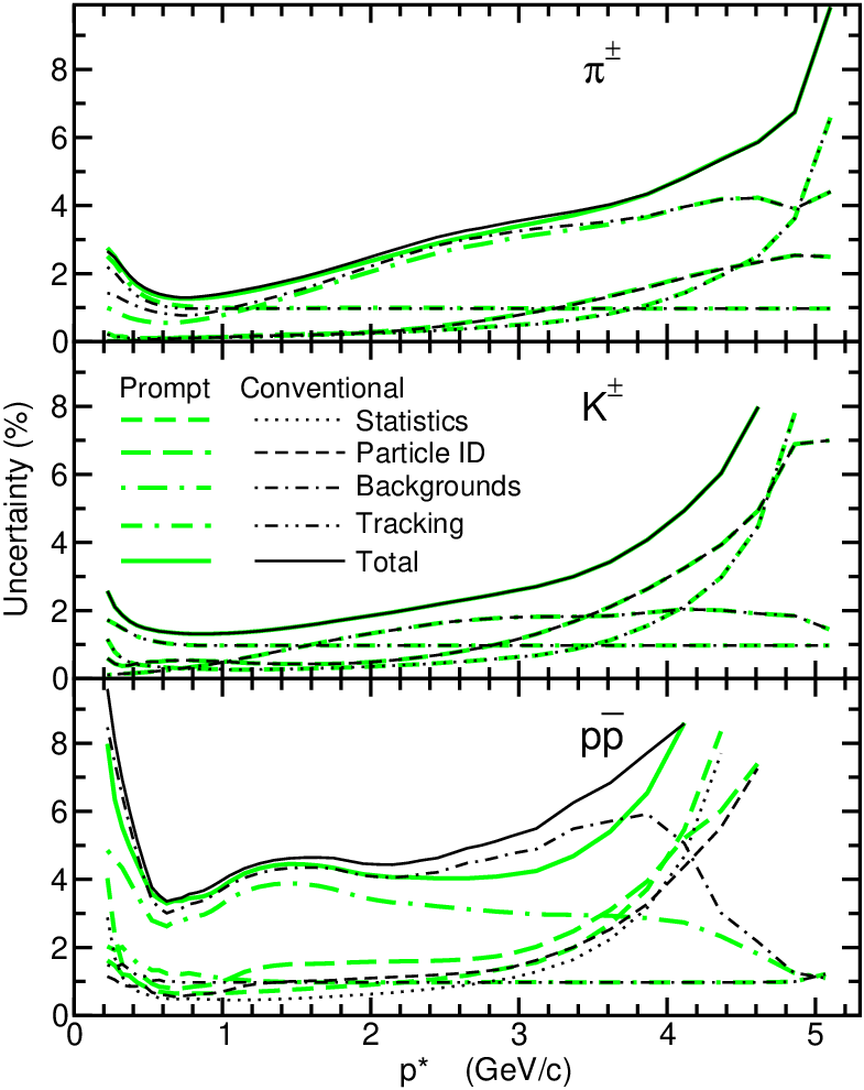
We summarize the relative uncertainties on our cross sections in Fig. 11. A few become large at high , where the cross sections become low, and we do not show those that are off the vertical scale. The statistical uncertainties are much smaller than the systematic uncertainties except at the highest values, and on the lowest- points. The samples with full detector simulation are similar in size to the data samples, and the corresponding uncertainties (not shown) are the largest systematic uncertainties at the highest values. The total uncertainties are as small as 1.2%, 1.4%, and 3.2% (1.3%, 1.4%, and 3.6% ) for prompt (conventional) , and , respectively, in the 0.6–0.8 range. They increase at lower due mostly to tracking efficiency, and at higher due to particle identification and backgrounds. The latter are dominated by -pairs for and , and by strange decays for .
All of the systematic uncertainties have strong point-to-point correlations. There is an overall normalization uncertainty of 0.98% from the event selection and part of the track-finding efficiency, which does not affect the shape of any cross section. The uncertainties due to most backgrounds, strange particle decays, distributions, and leptons are correlated over wide ranges, and can have broad effects on the shape. Those due to particle identification are correlated strongly over short ranges, typically 1–2 neighboring bins, and more weakly over 2–4 additional bins, and the simulation has been smoothed so that its statistical uncertainty is correlated over 4–6 bins. These can lead to apparent structures in the cross sections over ranges of several bins. The remaining uncertainties on the tracking efficiencies and those due to interactions in the detector material (radiative Bhabha background) are fully correlated over the entire range, but are non-negligible only in the 6–10 lowest (highest) bins. Overall, the correlation coefficients for neighboring bins are 92–99% near the centers of the measured ranges and 72–96% (15–73%) toward the low-(high-) end. They are over 50% for bin separations of 12 or fewer. The full correlation matrices are given in the supplementary material [39].
VI Results and Interpretation
| Momentum | |||||||||||||
|---|---|---|---|---|---|---|---|---|---|---|---|---|---|
| Range () | value | stat. | syst. | Value | stat. | syst. | value | stat. | syst. | ||||
| 0.20 – | 0.25 | 8.01 | 0.02 | 0.22 | 0.291 | 0.003 | 0.007 | 0.0479 | 0.0019 | 0.0033 | |||
| 0.25 – | 0.30 | 8.25 | 0.01 | 0.21 | 0.382 | 0.003 | 0.007 | 0.0672 | 0.0016 | 0.0040 | |||
| 0.30 – | 0.35 | 8.04 | 0.01 | 0.17 | 0.468 | 0.003 | 0.008 | 0.0879 | 0.0013 | 0.0047 | |||
| 0.35 – | 0.40 | 7.52 | 0.01 | 0.14 | 0.538 | 0.003 | 0.009 | 0.1046 | 0.0012 | 0.0050 | |||
| 0.40 – | 0.45 | 6.93 | 0.01 | 0.11 | 0.591 | 0.002 | 0.009 | 0.1167 | 0.0011 | 0.0051 | |||
| 0.45 – | 0.50 | 6.36 | 0.01 | 0.10 | 0.633 | 0.002 | 0.009 | 0.1237 | 0.0011 | 0.0048 | |||
| 0.50 – | 0.55 | 5.78 | 0.01 | 0.08 | 0.669 | 0.002 | 0.009 | 0.1296 | 0.0010 | 0.0045 | |||
| 0.55 – | 0.60 | 5.21 | 0.01 | 0.07 | 0.682 | 0.002 | 0.009 | 0.1356 | 0.0009 | 0.0045 | |||
| 0.60 – | 0.65 | 4.69 | 0.01 | 0.06 | 0.689 | 0.002 | 0.009 | 0.1380 | 0.0009 | 0.0044 | |||
| 0.65 – | 0.70 | 4.21 | 0.01 | 0.05 | 0.687 | 0.002 | 0.009 | 0.1384 | 0.0009 | 0.0046 | |||
| 0.70 – | 0.75 | 3.781 | 0.005 | 0.048 | 0.676 | 0.002 | 0.009 | 0.1363 | 0.0009 | 0.0045 | |||
| 0.75 – | 0.80 | 3.402 | 0.004 | 0.043 | 0.658 | 0.002 | 0.008 | 0.1331 | 0.0009 | 0.0045 | |||
| 0.80 – | 0.85 | 3.065 | 0.004 | 0.039 | 0.636 | 0.002 | 0.008 | 0.1292 | 0.0008 | 0.0044 | |||
| 0.85 – | 0.90 | 2.765 | 0.004 | 0.035 | 0.616 | 0.002 | 0.008 | 0.1256 | 0.0008 | 0.0043 | |||
| 0.90 – | 0.95 | 2.495 | 0.003 | 0.032 | 0.593 | 0.002 | 0.008 | 0.1200 | 0.0008 | 0.0042 | |||
| 0.95 – | 1.00 | 2.258 | 0.003 | 0.030 | 0.568 | 0.002 | 0.007 | 0.1135 | 0.0008 | 0.0041 | |||
| 1.00 – | 1.10 | 1.948 | 0.002 | 0.027 | 0.531 | 0.001 | 0.007 | 0.1033 | 0.0007 | 0.0040 | |||
| 1.10 – | 1.20 | 1.603 | 0.002 | 0.023 | 0.482 | 0.001 | 0.006 | 0.0919 | 0.0006 | 0.0038 | |||
| 1.20 – | 1.30 | 1.332 | 0.002 | 0.020 | 0.435 | 0.001 | 0.006 | 0.0823 | 0.0006 | 0.0035 | |||
| 1.30 – | 1.40 | 1.106 | 0.002 | 0.018 | 0.389 | 0.001 | 0.006 | 0.0734 | 0.0005 | 0.0032 | |||
| 1.40 – | 1.50 | 0.926 | 0.002 | 0.016 | 0.347 | 0.001 | 0.005 | 0.0655 | 0.0005 | 0.0029 | |||
| 1.50 – | 1.60 | 0.780 | 0.002 | 0.014 | 0.3080 | 0.0009 | 0.0047 | 0.0588 | 0.0005 | 0.0026 | |||
| 1.60 – | 1.70 | 0.659 | 0.001 | 0.013 | 0.2731 | 0.0008 | 0.0043 | 0.0526 | 0.0004 | 0.0023 | |||
| 1.70 – | 1.80 | 0.559 | 0.001 | 0.012 | 0.2427 | 0.0008 | 0.0040 | 0.0466 | 0.0004 | 0.0020 | |||
| 1.80 – | 1.90 | 0.475 | 0.001 | 0.010 | 0.2161 | 0.0007 | 0.0037 | 0.0416 | 0.0004 | 0.0017 | |||
| 1.90 – | 2.00 | 0.404 | 0.001 | 0.009 | 0.1921 | 0.0007 | 0.0034 | 0.0374 | 0.0003 | 0.0015 | |||
| 2.00 – | 2.10 | 0.343 | 0.001 | 0.008 | 0.1698 | 0.0006 | 0.0031 | 0.0331 | 0.0003 | 0.0013 | |||
| 2.10 – | 2.20 | 0.294 | 0.001 | 0.007 | 0.1503 | 0.0006 | 0.0029 | 0.0293 | 0.0003 | 0.0012 | |||
| 2.20 – | 2.30 | 0.251 | 0.001 | 0.007 | 0.1323 | 0.0005 | 0.0026 | 0.0259 | 0.0003 | 0.0010 | |||
| 2.30 – | 2.40 | 0.216 | 0.001 | 0.006 | 0.1167 | 0.0005 | 0.0024 | 0.0227 | 0.0002 | 0.0009 | |||
| 2.40 – | 2.50 | 0.186 | 0.001 | 0.005 | 0.1031 | 0.0005 | 0.0022 | 0.0201 | 0.0002 | 0.0008 | |||
| 2.50 – | 2.60 | 0.1610 | 0.0006 | 0.0048 | 0.0909 | 0.0004 | 0.0020 | 0.0176 | 0.0002 | 0.0007 | |||
| 2.60 – | 2.70 | 0.1394 | 0.0005 | 0.0043 | 0.0802 | 0.0004 | 0.0018 | 0.0154 | 0.0002 | 0.0006 | |||
| 2.70 – | 2.80 | 0.1213 | 0.0005 | 0.0038 | 0.0704 | 0.0004 | 0.0016 | 0.0133 | 0.0002 | 0.0005 | |||
| 2.80 – | 2.90 | 0.1048 | 0.0005 | 0.0034 | 0.0622 | 0.0004 | 0.0015 | 0.01146 | 0.00015 | 0.00044 | |||
| 2.90 – | 3.00 | 0.0910 | 0.0004 | 0.0030 | 0.0546 | 0.0003 | 0.0014 | 0.00979 | 0.00014 | 0.00038 | |||
| 3.00 – | 3.25 | 0.0706 | 0.0004 | 0.0024 | 0.0436 | 0.0003 | 0.0011 | 0.00733 | 0.00011 | 0.00029 | |||
| 3.25 – | 3.50 | 0.0497 | 0.0003 | 0.0018 | 0.0306 | 0.0003 | 0.0009 | 0.00448 | 0.00009 | 0.00019 | |||
| 3.50 – | 3.75 | 0.0350 | 0.0003 | 0.0014 | 0.0209 | 0.0002 | 0.0007 | 0.00260 | 0.00007 | 0.00012 | |||
| 3.75 – | 4.00 | 0.0246 | 0.0003 | 0.0010 | 0.0139 | 0.0002 | 0.0005 | 0.00143 | 0.00005 | 0.00008 | |||
| 4.00 – | 4.25 | 0.0167 | 0.0002 | 0.0008 | 0.00910 | 0.00019 | 0.00041 | 0.00073 | 0.00004 | 0.00005 | |||
| 4.25 – | 4.50 | 0.0107 | 0.0002 | 0.0005 | 0.00568 | 0.00017 | 0.00030 | 0.00036 | 0.00003 | 0.00003 | |||
| 4.50 – | 4.75 | 0.00681 | 0.00017 | 0.00036 | 0.00324 | 0.00015 | 0.00021 | 0.00017 | 0.00002 | 0.00002 | |||
| 4.75 – | 5.00 | 0.00418 | 0.00015 | 0.00024 | 0.00149 | 0.00012 | 0.00015 | 0.00007 | 0.00002 | 0.00001 | |||
| 5.00 – | 5.27 | 0.00153 | 0.00010 | 0.00011 | 0.00050 | 0.00007 | 0.00007 | 0.00001 | 0.00001 | 0.00001 | |||
| 0.20 – | 5.27 | 5.364 | 0.002 | 0.080 | 0.946 | 0.001 | 0.012 | 0.1819 | 0.0003 | 0.0058 | |||
| Momentum | |||||||||||||
|---|---|---|---|---|---|---|---|---|---|---|---|---|---|
| Range () | value | stat. | syst. | Value | stat. | syst. | value | stat. | syst. | ||||
| 0.20 – | 0.25 | 9.25 | 0.02 | 0.24 | 0.291 | 0.003 | 0.007 | 0.068 | 0.002 | 0.006 | |||
| 0.25 – | 0.30 | 9.45 | 0.01 | 0.23 | 0.383 | 0.003 | 0.007 | 0.094 | 0.002 | 0.007 | |||
| 0.30 – | 0.35 | 9.14 | 0.01 | 0.20 | 0.468 | 0.003 | 0.008 | 0.122 | 0.001 | 0.008 | |||
| 0.35 – | 0.40 | 8.51 | 0.01 | 0.16 | 0.538 | 0.003 | 0.009 | 0.145 | 0.001 | 0.009 | |||
| 0.40 – | 0.45 | 7.82 | 0.01 | 0.14 | 0.591 | 0.002 | 0.009 | 0.161 | 0.001 | 0.008 | |||
| 0.45 – | 0.50 | 7.15 | 0.01 | 0.11 | 0.633 | 0.002 | 0.009 | 0.171 | 0.001 | 0.007 | |||
| 0.50 – | 0.55 | 6.47 | 0.01 | 0.10 | 0.669 | 0.002 | 0.009 | 0.180 | 0.001 | 0.007 | |||
| 0.55 – | 0.60 | 5.83 | 0.01 | 0.08 | 0.683 | 0.002 | 0.009 | 0.188 | 0.001 | 0.007 | |||
| 0.60 – | 0.65 | 5.23 | 0.01 | 0.07 | 0.689 | 0.002 | 0.009 | 0.192 | 0.001 | 0.006 | |||
| 0.65 – | 0.70 | 4.69 | 0.01 | 0.06 | 0.687 | 0.002 | 0.009 | 0.193 | 0.001 | 0.007 | |||
| 0.70 – | 0.75 | 4.21 | 0.01 | 0.05 | 0.677 | 0.002 | 0.009 | 0.191 | 0.001 | 0.007 | |||
| 0.75 – | 0.80 | 3.778 | 0.004 | 0.049 | 0.658 | 0.002 | 0.008 | 0.187 | 0.001 | 0.007 | |||
| 0.80 – | 0.85 | 3.401 | 0.004 | 0.044 | 0.636 | 0.002 | 0.008 | 0.183 | 0.001 | 0.007 | |||
| 0.85 – | 0.90 | 3.067 | 0.004 | 0.041 | 0.616 | 0.002 | 0.008 | 0.179 | 0.001 | 0.007 | |||
| 0.90 – | 0.95 | 2.768 | 0.003 | 0.038 | 0.593 | 0.002 | 0.008 | 0.173 | 0.001 | 0.006 | |||
| 0.95 – | 1.00 | 2.504 | 0.003 | 0.035 | 0.568 | 0.002 | 0.007 | 0.165 | 0.001 | 0.006 | |||
| 1.00 – | 1.10 | 2.159 | 0.003 | 0.031 | 0.531 | 0.001 | 0.007 | 0.153 | 0.001 | 0.006 | |||
| 1.10 – | 1.20 | 1.775 | 0.002 | 0.027 | 0.482 | 0.001 | 0.006 | 0.139 | 0.001 | 0.006 | |||
| 1.20 – | 1.30 | 1.472 | 0.002 | 0.024 | 0.435 | 0.001 | 0.006 | 0.126 | 0.001 | 0.006 | |||
| 1.30 – | 1.40 | 1.221 | 0.002 | 0.021 | 0.389 | 0.001 | 0.006 | 0.113 | 0.001 | 0.005 | |||
| 1.40 – | 1.50 | 1.020 | 0.002 | 0.018 | 0.347 | 0.001 | 0.005 | 0.1006 | 0.0005 | 0.0046 | |||
| 1.50 – | 1.60 | 0.857 | 0.002 | 0.016 | 0.3080 | 0.0009 | 0.0047 | 0.0900 | 0.0005 | 0.0042 | |||
| 1.60 – | 1.70 | 0.723 | 0.001 | 0.015 | 0.2731 | 0.0008 | 0.0043 | 0.0799 | 0.0004 | 0.0037 | |||
| 1.70 – | 1.80 | 0.611 | 0.001 | 0.013 | 0.2427 | 0.0008 | 0.0040 | 0.0704 | 0.0004 | 0.0032 | |||
| 1.80 – | 1.90 | 0.518 | 0.001 | 0.012 | 0.2161 | 0.0007 | 0.0037 | 0.0620 | 0.0004 | 0.0028 | |||
| 1.90 – | 2.00 | 0.439 | 0.001 | 0.011 | 0.1921 | 0.0007 | 0.0034 | 0.0548 | 0.0003 | 0.0024 | |||
| 2.00 – | 2.10 | 0.372 | 0.001 | 0.009 | 0.1698 | 0.0006 | 0.0031 | 0.0480 | 0.0003 | 0.0021 | |||
| 2.10 – | 2.20 | 0.317 | 0.001 | 0.008 | 0.1503 | 0.0006 | 0.0029 | 0.0419 | 0.0003 | 0.0018 | |||
| 2.20 – | 2.30 | 0.270 | 0.001 | 0.008 | 0.1323 | 0.0005 | 0.0026 | 0.0364 | 0.0003 | 0.0016 | |||
| 2.30 – | 2.40 | 0.231 | 0.001 | 0.007 | 0.1167 | 0.0005 | 0.0024 | 0.0315 | 0.0002 | 0.0014 | |||
| 2.40 – | 2.50 | 0.198 | 0.001 | 0.006 | 0.1031 | 0.0005 | 0.0022 | 0.0275 | 0.0002 | 0.0012 | |||
| 2.50 – | 2.60 | 0.170 | 0.001 | 0.005 | 0.0909 | 0.0004 | 0.0020 | 0.0237 | 0.0002 | 0.0011 | |||
| 2.60 – | 2.70 | 0.1471 | 0.0006 | 0.0048 | 0.0802 | 0.0004 | 0.0018 | 0.0206 | 0.0002 | 0.0010 | |||
| 2.70 – | 2.80 | 0.1276 | 0.0005 | 0.0042 | 0.0704 | 0.0004 | 0.0016 | 0.0176 | 0.0002 | 0.0009 | |||
| 2.80 – | 2.90 | 0.1099 | 0.0005 | 0.0037 | 0.0622 | 0.0004 | 0.0015 | 0.0150 | 0.0002 | 0.0008 | |||
| 2.90 – | 3.00 | 0.0950 | 0.0004 | 0.0033 | 0.0546 | 0.0003 | 0.0014 | 0.0128 | 0.0001 | 0.0007 | |||
| 3.00 – | 3.25 | 0.0734 | 0.0004 | 0.0026 | 0.0436 | 0.0003 | 0.0011 | 0.00926 | 0.00012 | 0.00049 | |||
| 3.25 – | 3.50 | 0.0513 | 0.0003 | 0.0019 | 0.0306 | 0.0003 | 0.0009 | 0.00564 | 0.00009 | 0.00034 | |||
| 3.50 – | 3.75 | 0.0359 | 0.0003 | 0.0014 | 0.0209 | 0.0002 | 0.0007 | 0.00324 | 0.00007 | 0.00021 | |||
| 3.75 – | 4.00 | 0.0251 | 0.0003 | 0.0011 | 0.0139 | 0.0002 | 0.0005 | 0.00173 | 0.00005 | 0.00012 | |||
| 4.00 – | 4.25 | 0.0169 | 0.0002 | 0.0008 | 0.00910 | 0.00019 | 0.00041 | 0.00087 | 0.00004 | 0.00006 | |||
| 4.25 – | 4.50 | 0.0108 | 0.0002 | 0.0005 | 0.00568 | 0.00017 | 0.00030 | 0.00040 | 0.00003 | 0.00003 | |||
| 4.50 – | 4.75 | 0.00682 | 0.00017 | 0.00036 | 0.00324 | 0.00015 | 0.00021 | 0.00017 | 0.00002 | 0.00002 | |||
| 4.75 – | 5.00 | 0.00418 | 0.00015 | 0.00024 | 0.00149 | 0.00012 | 0.00015 | 0.00007 | 0.00002 | 0.00001 | |||
| 5.00 – | 5.27 | 0.00153 | 0.00010 | 0.00011 | 0.00050 | 0.00007 | 0.00007 | 0.00001 | 0.00001 | 0.00001 | |||
| 0.20 – | 5.27 | 6.002 | 0.002 | 0.092 | 0.946 | 0.001 | 0.012 | 0.2612 | 0.0003 | 0.0095 | |||
Our results for prompt and conventional hadrons are listed in Tables 1 and 2. Several other tables, including breakdowns of the uncertainties and their correlations, are available in the supplementary material [39]. In this section, we compare the cross section results with previous measurements, models of hadronization, and predictions of QCD. We also calculate average event multiplicities, ratios of differential production cross sections, and charged hadron fractions.
VI.1 Cross Sections in Events
We compare our results with previous measurements from the ARGUS experiment [11] of differential , and production cross sections in events at the slightly lower . Figure 12 shows their tabulated results for prompt particles, along with ours, in terms of the scaled momentum , over the range of their measurements. Total uncertainties are shown for both data sets. Although our results are far more precise statistically, the systematic uncertainties are comparable and are correlated over significant ranges in both cases. The ARGUS and data extend to lower values, whereas ours extend up to , so that most of the relevant range is covered between the two experiments.

For , the two data sets are consistent. As decreases, the ARGUS data fall systematically below ours, as might be expected from a mass-driven scaling violation. The differences are consistent with those expected by the hadronization models described in Sec. VI.2. However, when the correlations between the systematic uncertainties are taken into account, the significance of these differences is only a few standard deviations for and , and below 2 for . ARGUS also presents results including and decay products. A comparison with our conventional results yields the same conclusions.
VI.2 Comparison with Hadronization Models
In Fig. 13, we compare our cross sections for prompt particles with the predictions of the three hadronization models discussed in Sec. I. These models represent the three different mechanisms for hadronization currently available. In each case we use the default parameter values, which have been chosen based on previous data, mostly at higher energies but including the ARGUS data. All three models describe the bulk of the spectra qualitatively, but no model describes any spectrum in detail. The peak positions are consistent with the data, except for the HERWIG , which is too low. The peak amplitudes are low by 9–20% for , high by 8–11% for , and either 30% low or 30–50% high for .

The HERWIG peaks are too narrow, and the high- tails are much too long; in particular, the spectrum shows a pronounced structure at high , and also drops to zero in the highest- bin. In contrast, the JETSET and UCLA and peaks are slightly too broad, and the tails too short, although both models describe the shape well in the 0.2–0.7 range. UCLA also reproduces the amplitude of the spectrum in this range. JETSET’s spectrum has the correct shape for , but then drops too slowly. UCLA’s spectrum is distorted relative to the data in a manner similar to HERWIG’s and spectra. A comparison of the conventional cross sections (not shown) gives similar results.
Similar discrepancies with these models have been reported at higher energies [12, 13, 14, 15, 16, 17, 18], although earlier versions of the models were often used and some parameter values differed. Most differences from the data were of the same sign and similar in size to those we observe, suggesting that the scaling with might be well simulated. In some cases, simple changes to parameters in JETSET produced improvements in the agreement with data, and some experiments implemented global tuning. We do not attempt to tune any of the models, but we test some simple modifications of JETSET parameters: changing the probability of producing a diquark-antidiquark, rather than a , pair at each string break modifies the amplitude of the simulated proton spectrum, but does not change the shape; similarly, the probability to produce an , rather than or , pair controls the amplitude, but not the shape, of the kaon spectrum.


We test the scaling properties of the models by generating samples with each at various energies, comparing them with available data, and looking for changes in the type or magnitude of any differences. In the top plot in Fig. 14 we show our conventional cross section along with those from the TASSO and SLD experiments. At high , these two experiments provide the most precise data and/or widest coverage for near 30 and the peak. Data from other experiments are consistent and yield the same conclusions, but are omitted for clarity. Strong scaling violations are evident, both at low due to the pion mass and at high as expected from the running of the strong coupling strength . Also shown are the predictions of the JETSET model at these three energies, using default parameter values. JETSET provides a good description of all three data sets for , and hence describes the high- scaling violation well. The other two models also reproduce this dependence, though they do not describe the spectrum well at any energy.
The middle plot in Fig. 14 shows a similar test for the cross section. Here we show the UCLA model predictions, as they describe our results best at high . The different flavor composition of the three samples is important for and modifies the expected scaling violation. Kaons from events, which are absent from our data, contribute strongly to the TASSO cross section in the 0.1–0.3 region, but little at higher . Since the cross sections are normalized per event, the expected scaling violation is reduced relative to that in the cross sections in the 0.1–0.3 range, and increased at higher . At the energy, the relative production of up- and down-type quarks is quite different, and the combination of more from and events and fewer from events pushes the simulated high- cross section up to nearly the same level as for the TASSO energy.
The flavor dependence has been shown [18, 15] to be accurately modeled at the energy to the level of about 10%. The UCLA model describes the shape of the SLD cross section at high well, but is too low by about 15%. The other models also predict about 15% more scaling violation than is observed. However, it is difficult to draw any conclusion in light of the flavor dependence.
For protons, shown in the bottom plot in Fig. 14, we compare with the JETSET model in which we have changed one parameter value, the diquark production probability , from 0.1 to 0.085. This provides a good description of the SLD and TASSO data at all , although the latter are sparse at high . The simulated high- scaling violation between 10.54 and 34 is similar to that for , but that between 34 and 91 is slightly larger since fast protons are expected to be produced predominantly in and events. The prediction for 10.54 is consistent with the BABAR data for below 0.07, but then rises well above the data, exceeding it by as much as a factor of 3 at . We see similar behavior for JETSET with default parameter values, HERWIG, and UCLA. Thus none of these models predicts the correct scaling properties for protons, even though they describe the properties of pions well.
VI.3 Tests of MLLA QCD
We test the predictions of QCD in the modified leading logarithm approximation (MLLA) [3], combined with the ansatz of local parton-hadron duality (LPHD) [3], using our cross sections in the variable . Figure 15 shows the distributions for prompt particles; the conventional distributions are similar in shape. The error bars are statistical. Because of their strong correlations, the systematic uncertainties are shown as bands. The normalization uncertainty is not included, as it does not affect the shapes.
This representation emphasizes the low- (large ) region and most of each spectrum is visible on a linear vertical scale. The spectra exhibit slow rises from zero at (the beam momentum) and the “humpbacked plateau” predicted by MLLALPHD. The MLLALPHD hypothesis also predicts that Gaussian functions should describe these spectra over ranges of 0.5–1 units about the peak position , and that slightly distorted Gaussian functions should fit the data over substantially wider ranges. Furthermore, should decrease exponentially with increasing hadron mass at a given , and increase logarithmically with for a given hadron type.

Following convention, we first estimate by fitting Gaussian functions over a set of ranges each about one unit wide and centered within one bin of the peak. Given our binning, we consider nine such ranges for , and four for and . We average the mean values and statistical and systematic uncertainties of the set of fits, and include the RMS deviation among the means as an additional systematic uncertainty. The fits use the full systematic error matrix and all have acceptable ; the resulting values are listed in Table 3 with their total uncertainties. The statistical uncertainties are negligible, and the RMS uncertainties are small except for the , where they are about half the other systematics. Adding more ranges to any set of fits has little effect on the results.
| Prompt | 2.3370.009 | 1.6220.006 | 1.6470.019 |
|---|---|---|---|
| Conventional | 2.3530.009 | 1.6220.006 | 1.6040.013 |
To test the prediction regarding the Gaussian shape, we first find the largest range centered near over which the Gaussian fit is acceptable, i.e., yields a with a confidence level exceeding 0.01. We then extend the fit range to either lower or higher values, if possible, to find a maximum range over which this function gives an acceptable fit. These ranges are listed in Table 4 and the fits are shown as the lines on Fig. 15. In each case we obtain a good fit over a range more than one unit wide, consistent with the prediction. For and the maximum ranges are centered near the peak and span nearly two units in width. The maximum range for pions extends to the end of our coverage, which is just under one unit above the peak. It extends more than 1.5 units below the peak, but data at higher might constrain this more tightly.
| Prompt | Conventional | |||||||||
| Hadron | Gaussian | Distorted | Gaussian | Distorted | ||||||
| 0.92–3.27 | 0.22–3.27 | 0.87–3.27 | 0.67–3.27 | |||||||
| 0.63–2.58 | 0.34–3.05 | 0.63–2.58 | 0.34–3.05 | |||||||
| 0.56–3.27 | 0.48–3.27 | 0.71–2.58 | 0.48–3.27 | |||||||
Next, we add approximate skewness () and kurtosis () terms to our fitting function, following Ref. [43]:
where , and is the standard deviation. We repeat the exercise of finding the maximum range for which a fit of this function is acceptable. The results are listed in Table 4 and shown as the dashed lines on Fig. 15. The prompt (conventional) range can be extended to substantially (somewhat) lower values, consistent with the prediction. However, the fitted skewness and kurtosis values increase rapidly as the range is extended, to 0.37 (0.11) and 0.43 (0.30), respectively, at the widest range, and it is unknown how additional data on the high side of the peak might affect the fits. The and ranges can be extended somewhat in both directions with similar and values. Given our relatively low and hence narrow range, this should also be considered consistent with the prediction.
We find to be 0.8 units higher than , consistent with the predicted decrease with hadron mass, but is not lower than . This is similar to the behavior observed at higher energies where mesons and baryons appear to follow different trajectories, but measurements for more particles at our would be needed to draw firm conclusions. In Fig. 16 we show a compilation of measurements for , and as a function of CM energy. Our precise values and those from the provide strong constraints on the trajectories, and the lines on the plot simply join the points at these two energies. The other data are consistent with the lines, and hence with the predicted energy dependence, but more precise data at other energies are needed to test the form of the increase. The slopes of the lines for pions and protons are similar, but that for the kaons is quite different. This could be due to the changing flavor composition.

VI.4 Average Multiplicities, Ratios and Fractions
To estimate the average numbers of pions, kaons and protons produced per event, we integrate the differential cross sections over the measured range, and correct for the unmeasured parts of the spectra. The integrals take all systematic uncertainties and their correlations into account, and are listed in the second column of Table 5. The uncertainties are dominated by the normalization and fully correlated tracking systematics; there are also substantial contributions to the conventional and results from the and strange baryon cross sections.
| Measured | Yield per Event | |||||||||||
|---|---|---|---|---|---|---|---|---|---|---|---|---|
| Particle | Integral | Coverage | BABAR | CLEO | ARGUS | JETSET | UCLA | HERWIG | ||||
| 5.51 | 0.08 | 0.8760.018 | 6.29 | 0.09 | 0.13 | 5.84 | 5.88 | 5.73 | ||||
| Prompt | 5.36 | 0.08 | 0.8840.019 | 6.07 | 0.09 | 0.13 | 5.6940.108 | 5.59 | 5.62 | 5.49 | ||
| 0.946 | 0.012 | 0.9730.016 | 0.972 | 0.012 | 0.016 | 0.8880.030 | 1.01 | 1.02 | 1.01 | |||
| 0.182 | 0.006 | 0.9840.007 | 0.185 | 0.006 | 0.001 | 0.2120.017 | 0.28 | 0.14 | 0.31 | |||
| 6.15 | 0.10 | 0.8670.019 | 7.09 | 0.11 | 0.16 | 6.58 | 6.60 | 6.55 | ||||
| Conventional | 6.00 | 0.10 | 0.8740.020 | 6.87 | 0.11 | 0.16 | 8.30.4 | 6.380.12 | 6.33 | 6.34 | 6.31 | |
| 0.946 | 0.012 | 0.9730.016 | 0.972 | 0.012 | 0.016 | 1.30.2 | 0.8880.030 | 1.01 | 1.02 | 1.01 | ||
| 0.261 | 0.008 | 0.9840.008 | 0.265 | 0.008 | 0.002 | 0.400.06 | 0.2710.018 | 0.37 | 0.20 | 0.46 | ||
From Fig. 15, it is clear that the coverage, i.e. the fraction of the spectrum covered by our measurement, is over 95% for and . However, it is smaller for , and in no case is it clear a priori how to account for this reliably. We consider four estimates of our coverage, one from each of the three hadronization models and one from an ensemble of distorted Gaussian fits. We consider fits over all ranges that include the ten highest- points and give an acceptable calculated from only the bins above the peak plus the five bins just below the peak. The average of these four coverage values is given in the third column of Table 5, with an uncertainty that corresponds to their RMS deviation. The spread among the fits is smaller than this, as are variations obtained by running any simulation with different parameter values. We divide each measured integral by the corresponding coverage to obtain the average event multiplicity listed in column four of Table 5.
Previous results from CLEO at 10.49 [33] and ARGUS at 9.98 are also listed in Table 5, as are the predictions of the three hadronization models. Our prompt (conventional) rate is 7% (8%) and 2.0 (2.2) higher than the ARGUS rate. A difference of this size is expected from the difference. Our and rates are also slightly higher than the ARGUS rates. The CLEO rates are substantially higher than ours, but their uncertainties are large. With default parameter values, all three models give conventional rates close to the ARGUS value and 8-9% below ours, even though the simulations are run at our . The models predict rates that are slightly too high, and widely varying rates, none of which is consistent with the data. The total charged hadron rates from ARGUS and CLEO are among the main inputs to the tuning of these models.


From our cross sections we can derive production ratios for pairs of hadrons, in which many of the systematic uncertainties cancel at least partly. The remaining uncertainties are dominated by particle identification systematics. Previous experiments have presented this information in the form of the fractions of all charged hadrons that are pions, kaons and protons, , and . We show our fractions for prompt and conventional hadrons in Fig. 17, and tabulate them in the supplementary material [39]. The prompt and conventional fractions are quite similar, and converge at high . Strange hadron decay products cause the conventional and to be larger than their prompt counterparts at low , with correspondingly smaller.
The dominance of pions at low is expected due to their lower mass and the contributions from decays of heavier hadrons. The plateau values of and near , of about 0.35 and 0.08, respectively, might reflect the intrinsic relative production of strange particles and baryons in the hadronization process. The decrease of at high might be kinematic – a proton must be produced along with an antibaryon, and the mass of the pair is a large fraction of /2. The from events are also kinematically limited, whereas those from and events become more important as increases, until perhaps the very highest- bins.
The predictions of the three models are also shown, and do not describe the data well. JETSET and UCLA provide reasonable qualitative descriptions but underpredict and overpredict at high . In particular does not decrease early or quickly enough. HERWIG’s description of is poor, and this affects and , which might otherwise be described reasonably well.
VII Summary
We present measurements of the differential production cross sections for charged pions, kaons, and protons in annihilations at , both excluding (prompt) and including (conventional) decay products of mesons and weakly decaying strange baryons. The measurements cover the CM momentum () range from 0.2 to the beam momentum. Comparing with previous measurements at the nearby of 9.98 , we find consistency for in the 1–3 range, and evidence for scaling violations below 1 .
These data can be used to test and tune models of the hadronization process. We find that the JETSET, UCLA, and HERWIG models, which were tuned to previous data between 9.98 and 35 , reproduce the and spectra to within 15% over most of the range, but do not describe their shapes in detail. All three models provide poor descriptions of the spectra. Comparing the same models with data at higher , we find that they reproduce the high- scaling properties of the cross section to within a few percent and the spectrum to within 15%, but predict about twice the scaling violation observed for .
The shape of the spectrum predicted by MLLA QCD is consistent with our data in all cases, and the peak positions are lower for than , as predicted. However, the for are not lower than those for . This is consistent with the behavior observed at higher , where the predicted mass dependence holds for mesons and baryons separately, but not together. The predicted dependence is consistent with the world’s data, with the slopes being similar for and ; the slope is lower, perhaps due to the changing flavor composition with increasing .
We integrate over the measured ranges, and extrapolate into the unmeasured regions, to measure a total of , , and prompt (, , and conventional) , and , respectively, per hadronic event. We also provide hadron fractions, in which many of the systematic uncertainties cancel. These measurements are also consistent with previous results and provide additional information that can be used to test models.
Acknowledgements
We are grateful for the extraordinary contributions of our PEP-II colleagues in achieving the excellent luminosity and machine conditions that have made this work possible. The success of this project also relies critically on the expertise and dedication of the computing organizations that support BABAR. The collaborating institutions wish to thank SLAC for its support and the kind hospitality extended to them. This work is supported by the US Department of Energy and National Science Foundation, the Natural Sciences and Engineering Research Council (Canada), the Commissariat à l’Energie Atomique and Institut National de Physique Nucléaire et de Physique des Particules (France), the Bundesministerium für Bildung und Forschung and Deutsche Forschungsgemeinschaft (Germany), the Istituto Nazionale di Fisica Nucleare (Italy), the Foundation for Fundamental Research on Matter (The Netherlands), the Research Council of Norway, the Ministry of Education and Science of the Russian Federation, Ministerio de Economía y Competitividad (Spain), and the Science and Technology Facilities Council (United Kingdom). Individuals have received support from the Marie-Curie IEF program (European Union) and the A. P. Sloan Foundation (USA).
References
- [1] See, e.g., R.K. Ellis, D.A. Ross and A.E. Terrano, Nucl. Phys. B 178, 421 (1981).
- [2] See, e.g., S. Moretti, Phys. Lett. B 420, 367 (1998).
- [3] Y.I. Azimov, Y.L. Dokshitzer, V.A. Khoze, and S.I. Troian, Z. Phys. C 27, 65 (1985).
- [4] G. Marchesini and B.R. Webber, Nucl. Phys. B 238, 1 (1984).
- [5] S. Albino, B.A. Kniehl, and G. Kramer, Nucl. Phys. B 803, 42 (2008); D. de Florian, R. Sassot, and M. Stratmann, Phys. Rev. D 75, 114010 (2007); M. Hirai, S. Kumano, T.H. Nagai, and K. Sudoh, Phys. Rev. D 75, 094009 (2007).
- [6] See, e.g., A. Böhrer, Phys. Rep. 291, 107 (1997); G.D. Lafferty, P.J. Reeves and M.R. Whalley, J. Phys. G21, A1 (1995); D.H. Saxon, in High Energy Electron-Positron Physics Vol. 1, Eds. A. Ali and P. Söding, World Scientific (1988) 539.
- [7] G. Corcella et al., JHEP 0101, 010 (2001); G. Marchesini et al., Comput. Phys. Commun. 67, 465 (1992).
- [8] T. Sjöstrand, Comput. Phys. Commun. 82, 74 (1994).
- [9] S. Chun and C. Buchanan, Phys. Rep. 292, 239 (1998).
- [10] P. Abreu et al. (DELPHI Collaboration), Phys. Lett. B 398, 194 (1997).
- [11] H. Albrecht et al. (ARGUS Collaboration), Z. Phys. C 44, 547 (1989).
- [12] H. Aihara et al. (TPC-2Gamma Collaboration), Phys. Rev. Lett. 61, 1263 (1988).
- [13] W. Braunschweig et al. (TASSO Collaboration), Z. Phys. C 42, 189 (1989).
- [14] R. Itoh et al. (TOPAZ Collaboration), Phys. Lett. B 345, 335 (1995).
- [15] P. Abreu et al. (DELPHI Collaboration), Eur. Phys. J. C 5, 585 (1998).
- [16] R. Akers et al. (OPAL Collaboration), Z. Phys. C 63, 181 (1994).
- [17] D. Buskulic et al. (ALEPH Collaboration), Z. Phys. C 66, 355 (1995).
- [18] K. Abe et al. (SLD Collaboration), Phys. Rev. D 59, 052001 (1999); Phys. Rev. D 69, 072003 (2004).
- [19] P. Abreu et al. (DELPHI Collaboration), Eur. Phys. J. C 18 (2000) 203; [Erratum-ibid. C 25 (2002) 493].
- [20] M. Leitgab, et al. (Belle Collaboration), Phys. Rev. Lett. 111 (2013) 062002.
- [21] K. Abe et al. (SLD Collaboration), Phys. Rev. Lett. 78 (1997) 3442; [Erratum-ibid. 79 (1997) 959].
- [22] G. Abbiendi et al. (OPAL Collaboration), Eur. Phys. J. C 16, 407 (2000).
- [23] B. Aubert et al. (BABAR Collaboration), Nucl. Instr. Methods A 479, 1 (2002); arXiv:1305.3560 [hep-ex], submitted to Nucl. Instr. Methods.
- [24] I. Adam et al. (BABAR DIRC Collaboration), Nucl. Instr. Methods A 538, 281 (2005).
- [25] G.C. Fox and S. Wolfram, Phys. Rev. Lett. 41, 1581 (1978); Nucl. Phys. B 149, 413 (1979).
- [26] S. Brandt et al., Phys. Lett. 12, 57 (1964); E. Farhi, Phys. Rev. Lett. 39, 1587 (1977).
- [27] S. Agostinelli et al. (GEANT4 Collaboration), Nucl. Instr. Methods A 506, 250 (2003).
- [28] S. Jadach and Z. Was, Comput. Phys. Commun. 64, 267 (1991).
- [29] J. Beringer, et al. (Particle Data Group), Phys. Rev. D 86, 010001 (2012).
- [30] S. Jadach, W. Placzek, and B.F.L. Ward, Phys. Lett. B 390, 298 (1997).
- [31] H. Czyz and J.H. Kühn, Eur. Phys. J. C 18, 497 (2001).
- [32] H. Paar and M. Sivertz, (unpublished), based on V.M. Budnev, et al., Phys. Rep. 15, 181 (1975).
- [33] S. Behrends et al. (CLEO Collaboration), Phys. Rev. D 31, 2161 (1985).
- [34] H. Albrecht et al. (ARGUS Collaboration), Z. Phys. C 62, 371 (1994).
- [35] B.L. Hartfiel, Ph.D. Thesis, Univ. of California-Los Angeles (2004); SLAC-R-823 (unpublished).
- [36] T. Allmendinger et al., Nucl. Instr. Methods Phys. Res. Sect. A 704 (2013) 44.
- [37] S. Christ, Ph.D. Thesis, Universität Rostock (2003) (unpublished).
- [38] B. Aubert, et al. (BABAR Collaboration), Phys. Rev. D 72, 052006 (2005).
- [39] Tables of charged hadron fractions, uncertainties and correlation matrices are available through Phys. Rev.
- [40] M. Artuso et al. (CLEO Collaboration), Phys. Rev. D 70, 112001 (2004).
- [41] R. Seuster et al. (Belle Collaboration), Phys. Rev. D 73, 032002 (2006).
- [42] B. Aubert, et al. (BABAR Collaboration), Phys. Rev. D 75, 012003 (2007).
- [43] Y.L. Dokshitzer, V.A. Khoze, and S.I. Troian, Int. J. Mod. Phys. A 7, 1875 (1992); C.P. Fong and B.R. Webber, Phys. Lett. B 229, 289 (1989).