3D test particle simulations of the Galactic disks. The kinematical effects of the bar.

Below we give a detailed description of the individual components contributing to the axisymmetric part of the potential. Table 1 lists their characteristic parameters.

The bulge follows a Hernquist (1990) potential,

with $a_{\mathrm{b}}=1\ \mathrm{kpc}$. We choose two different values for the mass of the bulge (and, therefore, of the bar): $M_{\mathrm{b}}=10^{10}M_{\odot}$ (B1) and $M_{\mathrm{b}}=2\times 10^{10}M_{\odot}$ (B2, see Section 2.2).

We represent the thin and thick disk potentials with Miyamoto & Nagai (1975) models,

where “$i$” stands for “thin” or “thick”. The mass ratio between the two disks is $20\%$ and this gives a thick-to-thin disk density normalization of $\sim 10\%$ near the Sun, similarly to what is observed in our Galaxy (Jurić et al., 2008). We have chosen the Miyamoto-Nagai functional form to represent the disks because of their mathematical simplicity which results in computational convenience. Since in reality the Galactic disks follow more closely an exponential form in the density (Binney & Tremaine 2008), we set the characteristic parameters of the Miyamoto-Nagai model to resemble the gravitational potential of two exponential disks with radial scale lengths $R_{h}=3\ \mathrm{kpc}$ (for both disks) and vertical scale lengths $z_{\mathrm{thin}}=0.3\ \mathrm{kpc}$ and $z_{\mathrm{thick}}=1\ \mathrm{kpc}$. Although the potentials are similar, the forces differ. At $R=8\ \mathrm{kpc}$ the Miyamoto-Nagai thin disk overestimates the exponential disk vertical force $f_{z}$ up to $30\%$ at $\left|z\right|\lesssim 0.3\ \mathrm{kpc}$, while it underestimates the force by $\sim 15\%$ at $|z|\gtrsim 0.3\ \mathrm{kpc}$. The exponential thick disk force in the Miyamoto-Nagai model is underestimated $\sim 10-15\%$ at all heights we consider. These small differences in the force field can presumabxly be regarded as being smaller than the uncertainties in the true form and values of the characteristic parameters of the Milky Way gravitational field.

The dark halo follows the NFW potential (Navarro et al. 1997)

with $M_{\mathrm{h}}=8\times 10^{11}M_{\odot}$, $a_{\mathrm{h}}=15.84$ and $c=18$ (Battaglia et al. 2005).

The axisymmetric potential consisting of halo, thin and thick disks is referred as “A0” (and is the same for all models explored), while when the bulge is added we refer to A0+B1 or A0+B2 depending on the mass of the bulge.

The 3D bar used in our simulations is a Ferrers (1870) bar, whose density profile is given by

where $m^{2}\equiv a^{2}\left(x^{2}/a^{2}+y^{2}/b^{2}+z^{2}/c^{2}\right)$. We choose $n=2$ and explore two sets of axis lengths taken from Bissantz & Gerhard (2002) and López-Corredoira et al. (2007), respectively. We dub them “Galactic Bar” (GB) and “Long Bar” (LB), in the same fashion as Gardner & Flynn (2010). The bar parameters are listed in Table 2.

For the pattern speed of the bar we use the value $\Omega_{\mathrm{b}}=50\ \mathrm{km}\ \mathrm{s}^{-1}\ \mathrm{kpc}^{-1}$, i.e. in the range of current determinations, which is between $35$ and $60\ \mathrm{km}\ \mathrm{s}^{-1}\ \mathrm{kpc}^{-1}$ (Gerhard 2011). It is important to notice that the effects on the velocity distribution in a certain volume are mainly set by the proximity to the main resonances. This implies that a faster (slower) pattern speed yields similar effects as the original bar in outer (inner) volumes.

As anticipated, the bar potential grows adiabatically in the simulations. Specifically, each simulation starts with an axisymmetric potential (either A0+B1 or A0+B2), and the mass of the bulge is transferred to the bar using the function

which runs smoothly from $\eta(0)=0$ to $\eta(t_{1})=1$ (Dehnen 2000). In particular:

• •

  for $t\in[0,t_{1}]$, $M_{\mathrm{bar}}(t)=\eta(t)M_{\mathrm{b}}(0)$ and $M_{\mathrm{b}}(t)=[1-\eta(t)]M_{\mathrm{b}}(0)$,

• •

  for $t>t_{1}$, $M_{\mathrm{bar}}(t)=M_{\mathrm{b}}(0)$ and $M_{\mathrm{b}}(t)=0$.

In our models $M_{\mathrm{b}}(0)=M_{\mathrm{bar}}(t\geq t_{1})=10^{10}M_{\odot}$ (B1) and $M_{\mathrm{b}}(0)=M_{\mathrm{bar}}(t\geq t_{1})=2\times 10^{10}M_{\odot}$ (B2), which is consistent with the mass estimates by Dwek et al. (1995) and Zhao & Mao (1996).

In all our simulations the bar grows following Eq. (5), up to time $t_{1}$. The choice of $t_{1}$ is not particularly relevant, as it was shown in Minchev et al. (2010) that a longer growth time of the bar only linearly delays the effects of the bar (in this case, the formation of the kinematic structures). Throughout this paper we always use $t_{1}=2T_{\mathrm{bar}}\simeq 246\ \mathrm{Myr}$ as in Fux (2001), where $T_{\mathrm{bar}}=2\pi/\Omega_{\mathrm{b}}$.

In Fig. 1 we show the circular velocity curves of the components of A0 and of the bulge B2. In the same figure we plot the circular velocity of the $m=0$ term of the Fourier decomposition of the bar potential GB2 (GB with $M_{\mathrm{bar}}=2\times 10^{10}M_{\odot}$). Note that, although the total mass of the bulge and the bar are the same, inside $R=20\ \mathrm{kpc}$ their velocity curves (blue and purple lines, respectively) differ because the enclosed masses are different. While the Hernquist bulge extends to infinity, all the bar’s mass is confined inside a radius equal to its semi-major axis (see Eq. 4). As a consequence, when the bar growth has been completed, the resulting circular velocity curve has changed. For this reason, for our analysis we use the circular velocity curve $v_{\mathrm{c}}(R)$ obtained by adding the contributions of the dark halo, thin and thick disk and $m=0$ component of the bar potential (A0+GB2). This curve is represented by the black line in Fig. 1. We see how the total rotation curve is mostly influenced by the bar for approximately $R<5\ \mathrm{kpc}$, by the thin disk for $5\ \mathrm{kpc}<R<10\ \mathrm{kpc}$ and by the dark halo for $R>10\ \mathrm{kpc}$. The value of the circular velocity at Solar radius, and for $z=0$ is $v_{\mathrm{c}}(8\ \mathrm{kpc})\simeq 222\ \mathrm{km}\ \mathrm{s}^{-1}$ for A0+GB1 and $v_{\mathrm{c}}(8\ \mathrm{kpc})\simeq 234\ \mathrm{km}\ \mathrm{s}^{-1}$ for A0+GB2.

We use two sets of initial conditions for our simulations: ICTHIN and ICTHICK. ICTHIN mimics the typical kinematics and density distribution of the intermediate age population of the thin disk, while ICTHICK represents the thick disk. We generate low (LR) and high resolution (HR) realizations, that have $N=5\times 10^{7}$ and $N=10^{9}$ particles respectively. We perform HR simulations for our standard Galactic model (A0+GB2, see below), to help to distinguish the resonant features that are in the wings of the distribution and often hidden in the noise.

The positions $(R,\phi,z)$ of the particles in both disks are distributed following Miyamoto-Nagai densities, corresponding to the potentials described in Section 2.1. The density distribution of each disk, $\rho_{\mathrm{d},i}$, is derived from Eq. (2) through Poisson’s equation (for the complete expression see Miyamoto & Nagai 1975). The $(R,z)$ positions of the particles are randomly drawn from these profiles with a method based on the Von Neumann’s rejection technique (Press et al. 1992) and $\varphi$ is generated uniformly between $0$ and $2\pi$.

Once the positions are generated, the velocities are assigned in the following way. We describe the radial velocity dispersion $\sigma_{R,i}$, as

(Hernquist 1993), which implies that, far enough from the center, $\sigma_{R,i}^{2}\propto\exp(-R/R_{\mathrm{h}})$. In the center the smoothing parameter $a_{\mathrm{s}}$ reduces the velocity dispersion. Hernquist (1993) uses $a_{\mathrm{s}}=R_{\mathrm{h}}/4$. We prefer $a_{\mathrm{s}}=R_{\mathrm{h}}$, which makes the smoothing much more gradual. We relate the tangential velocity dispersion $\sigma_{\phi,i}$ to the radial $\sigma_{R,i}$ through the epicyclic approximation, i.e.,

where $\Omega(R)$ and $\kappa(R)$ are the circular and epicyclic frequencies (Binney & Tremaine 2008).

Finally, the vertical velocity dispersion $\sigma_{z,i}$ is obtained by solving the following Jeans equation for an axisymmetric system

where $\Phi(R,z)$ is the total potential of the Galaxy. Assuming a velocity ellipsoid aligned with the $R$ and $z$ axes, i.e., $(\overline{v_{R}v_{z}})_{i}=0$, the first term in the left-hand side of Eq. (8) vanishes, and

In practice, we compute Eq. (9) on a discrete grid of equispaced points on the meridional plane and, to obtain $\sigma_{z,i}(R,z)$ in a generic $(R,z)$ point, we linearly interpolate between the nearest grid points.

Each velocity component of a particle is assigned by drawing a random number from a Gaussian distribution with the respective dispersion. The tangential component of the velocity, $v_{\phi,i}$, is corrected for the asymmetric drift $v_{\mathrm{a},i}$,

(Binney & Tremaine 2008) where, again, we set $(\overline{v_{R}v_{z}})_{i}=0$.

The initial conditions generated in this way are not fully consistent with the potential. In particular we have assumed the velocity distribution to be locally Gaussian. Therefore we expect these to change in time, while reaching equilibrium with the potential. These transient effects are described in Minchev et al. (2009) and produce kinematic arcs in the Solar Neighbourhood. To avoid confusion between these effects and those induced by the bar we first let our initial conditions evolve in the axisymmetric potential for a time $t_{\mathrm{r}}$. We find that $t_{\mathrm{r}}\sim 8\ \mathrm{Gyr}$ suffices to reach a stationary state around and inside the Solar radius. We use these evolved initial conditions as effective initial conditions for our simulations with the bar.

The evolution of the velocity dispersions for ICTHIN and ICTHICK is shown in Fig. 2 for the axisymmetric potential A0+B2 (the results for A0+B1 are similar). We see that the radial and tangential velocity dispersions increase in the outer parts of the Galaxy and decrease in the inner regions, both for ICTHIN and ICTHICK. In contrast, the vertical velocity dispersion does not evolve for ICTHIN and only slightly increases for ICTHICK. This is likely because the vertical velocity dispersion is obtained directly by solving the Jeans equation, while the radial dispersion and tangential profiles are only imposed later using Eq. (7) and related through the epicyclic approximation .

An intermediate age population in the thin disk ($\sim 5\ \mathrm{Gyr}$) has local velocity dispersions $(\sigma_{R},\sigma_{\phi},\sigma_{z})\sim(40,26,17)\ \mathrm{km}\ \mathrm{s}^{-1}$ (Robin et al., 2003; Holmberg et al., 2007). After evolution, our set of initial conditions ICTHIN has comparable characteristics with slightly larger $\sigma_{\phi}$ and smaller $\sigma_{z}$. The measured local dispersions of the stars in the thick disc are $(\sigma_{R},\sigma_{\phi},\sigma_{z})\sim(67,51,42)\ \mathrm{km}\ \mathrm{s}^{-1}$ according to Robin et al. (2003) or smaller in the $\phi$ and $z$ directions $(\sigma_{R},\sigma_{\phi},\sigma_{z})\sim(67,38,35)\ \mathrm{km}\ \mathrm{s}^{-1}$ as reported in Bensby et al. (2003). Our initial conditions ICTHICK after the evolution in the imposed potential are consistent with these measurements.

Let us, for a moment, consider orbits in an axisymmetric potential. In the epicyclic approximation (that is a good description only of orbits that are almost circular and with small vertical motion amplitudes) the azimuthal velocity of a star, located at $R$ in the Galaxy, is

where $R_{\mathrm{g}}$ is the radius of the guiding center of its orbit. When higher order terms are considered, $v_{\phi}$ depends also on the value of $v_{R}$ (e.g., Dehnen 1999). Of particular interest are the orbits with $R_{\mathrm{g}}$ such that

where $l_{1}$ and $l_{2}$ are two integer numbers. For these orbits the epicyclic frequency resonates with the frequency of the circular orbit at $R_{\mathrm{g}}$, in the reference frame rotating with pattern speed $\Omega_{\mathrm{b}}$. In other words, orbits well described by the epicyclic approximation (i.e., not too eccentric) that satisfy this condition are closed in this reference frame. Important for the rest of the paper are, especially, the Outer Lindblad Resonance (OLR, $R_{\mathrm{g}}=R_{\mathrm{OLR}}$) where $l_{1}=-2$ and $l_{2}=1$, the $-1:1$ Resonance ($R_{\mathrm{g}}=R_{-1:1}$), where $l_{1}=-1$ and $l_{2}=1$, and the Corotation Resonance ($R_{\mathrm{g}}=R_{\mathrm{COR}}$), where $l_{2}=0$ (i.e., $\Omega(R_{\mathrm{g}})=\Omega_{\mathrm{b}}$). In Fig. 3 we show the positions of the main resonances for the A0 +GB2 potential but considering only the $m=0$ Fourier component of GB2, for $\Omega_{\mathrm{b}}=50\ \mathrm{km}\ \mathrm{s}^{-1}\ \mathrm{kpc}^{-1}$ (Table 2).

Now, let us assume a small non-axisymmetric perturbation (the bar) to the axisymmetric potential, rotating with pattern speed $\Omega_{\mathrm{b}}$. If the perturbation is small, the motion of most stars will still be approximately described by the epicyclic theory. However, some stars will be more strongly affected by the perturbation, namely those that satisfy Eq. (12) in the axisymmetric potential. As stated by Binney & Tremaine (2008), at the resonances the “perturbation is acting with one sign for a long time. If the effects of a perturbation can accumulate for long enough, they can become important, even if the perturbation is weak”.

The simple dynamical picture that we described in the previous section is complicated in two ways in the Milky Way: Galactic disks are 3D structures, i.e. stars have vertical motions, and especially the thick disk population is kinematically hot.

The epicyclic approximation assumes that the orbits of the stars are not too eccentric and that the amplitudes of the vertical motions are so small that horizontal and vertical motions are nearly decoupled. In an axisymmetric potential the motion is exactly decoupled when the radial and vertical force ($f_{R}$ and $f_{z}$) are respectively functions of $R$ and $z$ only. This is only true very near to the Galactic plane. In Fig. 4 we have plotted the radial (top) and vertical (bottom) forces for the total potential (colour) and the contribution of the bar ($m>0$ terms of the Fourier decomposition, black solid lines) for model A0+GB2. The bottom panel shows, as just discussed, that $f_{z}$ is independent of $R$ only at small $z$ (where it runs parallel to the cylindrical radius axis). However, already beyond $z\sim 0.3\ \mathrm{kpc}$, it varies significantly with $R$, over the range explored by many orbits that visit the Solar Neighbourhood. On the other hand, the top panel shows that the $f_{R}$ isocontours are less curved and that this force decreases more slowly with $z$ (and this is even more true if we consider the bar’s radial force only as indicated by the black curves). For this reason the radial motion may be expected to be more similar with height, than the vertical motion with radius. Furthermore, it is important also to note that orbits with angular momentum $L_{z}$ and vertical oscillations larger than $\sim 0.3\ \mathrm{kpc}$ live in a range of $R$ that is hundred of parsecs different from that of a planar orbit with the same $L_{z}$ angular momentum (see Binney & McMillan 2011).

Also interesting is that for all our models the bar induces horizontal forces that, at $R\sim 8\ \mathrm{kpc}$, are almost independent on $z$ (top panel of Fig. 4, solid black curves). In fact, the relative importance of the perturbation due to the bar slightly increases with $z$, as a consequence of the decreasing radial force of the axisymmetric part of the potential. Therefore, we expect stars far from the Galactic plane to experience a slightly stronger relative effect of the bar compared to those on the plane.

The exact details of how the vertical motions, particularly for the populations with larger kinematic temperature, affect the simple dynamical picture previously sketched, require however, as especially the bottom panel of Fig. 4 shows, suitable and fully 3D orbital integrations.

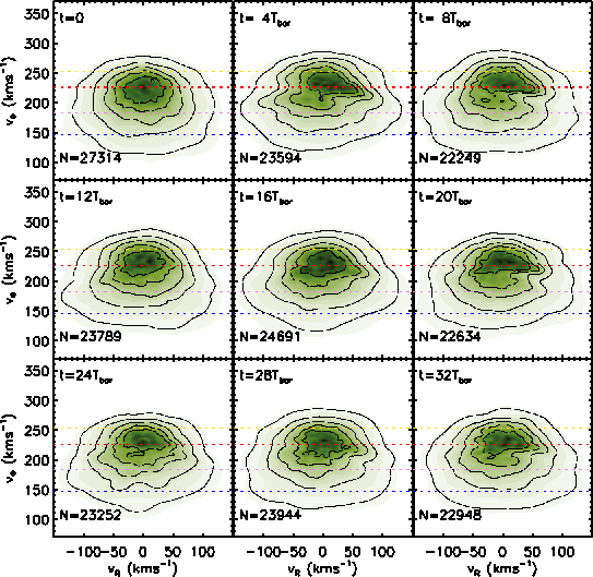
In Fig. 5 we show the evolution in time of the kinematics in the Solar Neighbourhood volume for the model A0+GB2 and the LR thin disk initial conditions (LR ICTHIN). Specifically, to describe the kinematics we use a probability density function of $(v_{R},v_{\phi})$, determined with the modified Breiman estimator, described in Ferdosi et al. (2011), with optimal pilot window $\sigma^{\mathrm{opt}}=9.6\ \mathrm{km}\ \mathrm{s}^{-1}$. We show $5$ density contours that enclose (from inside to outside) $0.25p_{1\sigma}\times i\ \%,\ i=1,...,5$ of the probability, where $p_{1\sigma}=68.268$. The $4$-th contour from inside out corresponds, therefore, to the $1\sigma$ contour. The evolution seen in Fig. 5 is qualitatively similar for all the other potentials (and respective values of the parameters) explored. As we can see, the form of the distribution changes with time (see Minchev et al. 2010 for a colder disk). Initially, the distribution of stars is featureless, symmetric in $v_{R}$, and with a tail of stars at low $v_{\phi}$ due to the asymmetric drift. At $t=4T_{\mathrm{bar}}$ the distribution has changed completely: it is split up in two regions and presents other deformations that make it asymmetric, both in $v_{R}$ and $v_{\phi}$.

Before proceeding with the analysis of the evolution in this plane, it will be useful for the rest of the paper to introduce a terminology describing the features seen in velocity space. In Fig. 5 we have indicated the $v_{\phi}$ of four important families of resonant orbits, using Eq. (11) for $R=8\ \mathrm{kpc}$: $v_{\phi,\mathrm{-1:1}}$ (yellow dashed line), $v_{\phi,\mathrm{OLR}}$ (red dashed line), $v_{\phi,\mathrm{-3:1}}$ (purple dashed line) and $v_{\phi,\mathrm{-4:1}}$ (blue dashed line). As we can see, the diagonal valley in the velocity distribution corresponds roughly to $v_{\phi,\mathrm{OLR}}$, confirming the large effect of the Outer Lindblad Resonance on the kinematics of the stars. Following Dehnen (2000), we call the peak in the density of stars above the valley the “LSR Mode”, and the one below the “OLR Mode”. Furthermore, in the right part of the LSR Mode, at $(v_{R},v_{\phi})\sim(75\ \mathrm{km}\ \mathrm{s}^{-1},220\ \mathrm{km}\ \mathrm{s}^{-1})$, there is an elongation in $v_{R}$, which we call “Horn”.

Previous studies have used default integration times of $t_{2}=4T_{\mathrm{bar}}$ (Dehnen 2000). We notice here that between $t=4T_{\mathrm{bar}}$ and $t=16T_{\mathrm{bar}}$ there is still significant evolution of the distribution, which only reaches a stationary configuration later. For instance, the valley between the LSR Mode and the OLR is progressively filled with stars. The OLR and LSR Modes change shape in time.

In general, it is clear from Fig. 5 that all the features associated to the bar are most prominent for short integration times. The features that we find in the velocity distribution for these times are similar to those observed by Dehnen (2000) in 2D integrations with a quadrupole bar. This is the first time that they are seen in 3D simulations. On the other hand, the time evolution confirms, again in 3D, the results obtained by Fux (2001) in his study of the phase-mixing of orbits in 2D and with the quadrupole bar.

As our thin disk corresponds to an intermediate-old population of stars, it is unlikely that they experienced the effects of the bar only for $4T_{\mathrm{bar}}$ ($\approx 492\ \mathrm{Myr}$). On the other hand, Cole & Weinberg (2002), using properties of infrared carbon stars from the Two Micron All Sky survey, state that the Milky Way Bar is likely to be younger than $3\ \mathrm{Gyr}$, fixing an upper limit for its formation to $6\ \mathrm{Gyr}$ ago (however studies of the bulge indicate that it is dominated by a stellar population older than $10\ \mathrm{Gyr}$, e.g., Minniti & Zoccali 2008). Given this, we decide to choose a default integration time of $t_{2}=24T_{\mathrm{bar}}\sim 3\ \mathrm{Gyr}$, when the kinematics have roughly reached stationarity. Note that we are effectively assuming that the properties of the bar, such as its pattern speed did not change much during this time.

Fig. 6 shows the kinematics of the thin disk in the Solar Neighbourhood and in two nearby volumes aligned with the Solar Neighbourhood ($\phi=-20^{\circ}$) but at different radii ($R=8.5\ \mathrm{kpc}$ and $R=7.5\ \mathrm{kpc}$) for various potentials and LR simulations. The first and second column show the distributions with the bar potential with $M_{\mathrm{bar}}=10^{10}M_{\odot}$ and $M_{\mathrm{bar}}=2\times 10^{10}M_{\odot}$, respectively. Not surprisingly, the effect of the least massive bar is weaker compared to a bar twice as massive. The density contrast between the OLR Mode and the LSR Mode is smaller, and the Horn is slightly less prominent for the least massive bar. The overall distribution has also a more symmetric appearance. These small differences are explainable by simply noting that the force of the perturbation only slightly smaller in the case of the least massive bar. The non-axisymmetric part of the force (i.e. excluding the monopole term associated to the bar) differs only by $\sim 30\%$ at $R=8\ \mathrm{kpc}$ between the GB1 and GB2. Some of the differences between the distributions may also be ascribed to the difference between the circular velocity curves of A0+B1 and A0+B2, which have the resonances at slightly different positions. For instance, for $\Omega_{\mathrm{b}}=50\ \mathrm{km}\ \mathrm{s}^{-1}\ \mathrm{kpc}^{-1}$, for A0+GB1 and for A0+GB2 (see Table 2). Since the resonances are mostly responsible for the effects of the bar on the kinematics of the stars, we expect some differences at fixed $R$ ²² 2 These differences may also reflect a dissimilar evolution of the distributions. As explained in Minchev et al. (2010), the typical time of libration of the stars trapped to the resonances depends on the bar strength; since the shape of the distributions is defined mostly by the resonances, we may expect, at the same snapshot, different evolutionary stages for different bar strengths..

The second and third columns of Fig. 6 allow us to compare more massive bar models ($M_{\mathrm{bar}}=2\times 10^{10}M_{\odot}$) with different geometrical properties (GB and LB). The Long Bar (third column) has slightly different effects on the thin disk velocity distributions than the less elongated Galactic Bar. It produces sharper features such as a Horn with a more defined lower edge, especially for $R=8.5\ \mathrm{kpc}$ and $R=8\ \mathrm{kpc}$. This was already noticed by Gardner & Flynn (2010) when they compared the responses to these two Ferrers bar models, but we confirm here their results in our 3D simulations. Nevertheless, we stress that, for this long integration time, the differences between the effect of the different bars on the kinematics inside the various volumes explored is much less significant than for shorter integration times. Furthermore, for short integration times the structures are much more evident in all our bar models.

Given the uncertainties in having a satisfactory model for the bar (recent studies even suggest that it could be a superposition of something similar to our Galactic Bar and Long Bar, see Robin et al. 2012), we use from now on as a default model the Galactic Bar and the potential A0+GB2, confident that the effects will be similar for all the other models, especially for long integration times, as illustrated in Fig. 6.

Since most works so far have used 2D simulations, it is important to understand if significant differences exist for the kinematics near the plane in the 2D vs 3D simulations. To this end we consider a subset of the HR 3D thin disk simulation in the potential A0+GB2, constituted by those particles that, at $t=0$, have $|z|<0.05\ \mathrm{kpc}$ and $|v_{z}|<5\ \mathrm{km}\ \mathrm{s}^{-1}$. These are the particles whose vertical oscillations have the smallest amplitude in the simulation: at $t=24T_{\mathrm{bar}}$ their $z$ dispersion is still less than $0.04\ \mathrm{kpc}$ and their $v_{z}$ dispersion less than $4\ \mathrm{km}\ \mathrm{s}^{-1}$. It is then reasonable to expect they behave in a similar fashion to particles in a 2D simulation, distributed on the Galactic plane with similar $(R,\phi)$ density and kinematics at $t=0$, and subject to the same potential A0+GB2.

Fig. 7 shows the kinematics of the subset of most “planar” particles (left panel) and the kinematics of a random subsample of the whole 3D simulation with the same number of stars (right panel), in the Solar Neighbourhood volume at the default integration time. We note that there are no large differences between the velocity distributions for these two data sets. The two sets do have slightly differing velocity dispersions: the planar particles are slightly colder ($\sigma_{R}=42\ \mathrm{km}\ \mathrm{s}^{-1}\ \mathrm{kpc}^{-1}$, while $\sigma_{R}=44\ \mathrm{km}\ \mathrm{s}^{-1}\ \mathrm{kpc}^{-1}$ for the 3D subsample), but this is a reflection of the initial conditions. This agreement stems likely from the fact that the planar and vertical motions are decoupled for most thin disk particles. Since our 3D thin disk is particularly cold in $v_{z}$ ($\sigma_{z}\sim 12\ \mathrm{km}\ \mathrm{s}^{-1}$ at $R=8\ \mathrm{kpc}$), it is also possible that this is more true in our simulations than in reality since the observed local $\sigma_{z}\sim 17\ \mathrm{km}\ \mathrm{s}^{-1}$ (Robin et al., 2003; Holmberg et al., 2007).

In Fig. 8 we show the kinematics of the thin disk in the vicinity of the Solar Neighbourhood at $t=24T_{\mathrm{bar}}$ and in HR. From left to right, the columns correspond to volumes centered at angles $\phi=-40^{\circ}$, $\phi=-20^{\circ}$ and $\phi=0$ (aligned with the bar). From bottom to top, the rows correspond to different Galactocentric radii from $R=7\ \mathrm{kpc}$ to $R=9\ \mathrm{kpc}$ in steps of $\Delta R=0.5\ \mathrm{kpc}$. The yellow, red, purple and blue dashed lines represent $v_{\phi}$ of the main resonances (as in Fig. 5), obtained by using Eq. (11) with the $R$ of the corresponding volume. This figure shows that the main kinematic features associated to the bar vary as a function of position in the Galaxy, similarly to the effects already reported in the literature for 2D simulations. First, we note that the main features shift in $v_{\phi}$ as $R$ varies. At $R=9\ \mathrm{kpc}$ (first row), $v_{\phi,\mathrm{OLR}}$ is in the low $v_{\phi}$ tail of the distribution ($v_{\phi}\sim 180\ \mathrm{km}\ \mathrm{s}^{-1}$), the OLR Mode has a small extension, and the Horn is placed at the lower right edge of the $1\sigma$ contour ($4$-th contour). For $R\sim 7.5$ and $8\ \mathrm{kpc}$ $v_{\phi,\mathrm{OLR}}$, and in consequence the separation between LSR Mode and OLR Mode, lies at the center of the $v_{\phi}$ distribution ($v_{\phi}\sim 220\ \mathrm{km}\ \mathrm{s}^{-1}$), and the LSR Mode and OLR Mode become clearly separated. For $R=7\ \mathrm{kpc}$ (bottom row), the LSR mode can hardly be seen and the Horn is now at the upper right edge of the distribution. Since these features are mostly associated with the resonant orbits, their shift can be explained in light of Eq. (11), for each of the resonant families ($R_{\mathrm{g}}$ constant).

We can also observe a change in the mean the $v_{R}$ of the OLR Mode as the orientation of the volume with respect to the bar ($\phi$) is varied. While the OLR Mode is almost completely symmetric with respect to the $v_{R}$ axis for $\phi=0$, it moves towards $v_{R}<0$ for more negative $\phi$. At $\phi=-40^{\circ}$ the OLR Mode is completely in the $v_{R}<0$ half plane at almost all radii. We quantify this change in Fig. 9. The red solid line shows the mean $v_{R}$ for particles with $v_{\phi}<v_{\phi,\mathrm{OLR}}$, in volumes at $R=8\ \mathrm{kpc}$ as function of $\phi$ (plotted in steps $\Delta\phi=2.5^{\circ}$). The black solid line represents the same quantity, but for the axisymmetric initial conditions and averaged between all the angles. The dashed lines represents twice the standard deviation of the set of means obtained for all the angles. This figure shows that the OLR Mode varies periodically in $v_{R}$ as a function of $\phi$, and that the amplitude of this oscillation is significantly above the noise level. Notice however how the curve is not perfectly symmetric: there is a wiggle for $-40^{\circ}<\phi<0$, and the amplitude is different between positive and negative $\langle v_{R}\rangle$. Because of the symmetry of the potential, we would expect instead $\langle v_{R}\rangle(\phi)=-\langle v_{R}\rangle(\pi-\phi)$, for each $\phi$. This happens because the disk has not reached a fully stationary equilibrium configuration at $R=8\ \mathrm{kpc}$ at this time (Fux 2001; Mühlbauer & Dehnen 2003). A much longer (and unrealistic) integration time of $120T_{\mathrm{bar}}$ ($\sim 15\ \mathrm{Gyr}$) is required to reach complete symmetry (Fig. 9, blue line). For volumes approximately aligned or perpendicular to the bar the OLR Mode has a null mean, that is the OLR Mode is centered. For these cases, however, the behaviour is still significantly different from the axisymmetric case, as one can see directly in the right column of Fig. 8, at $R=8\ \mathrm{kpc}$, where the bimodality, despite being centered with respect to $v_{R}$, is still present, and as shown in Fig. 10. In this figure we restrict the attention to those stars with $\left|v_{R}\right|<30\ \mathrm{km}\ \mathrm{s}^{-1}$, where the differences from the axisymmetric initial conditions are enhanced.

The vertex deviation $l_{v}$ quantifies the orientation of the velocity ellipsoid on the $z=0$ plane. Following Binney & Merrifield (1998) this is:

The corresponding values are quoted in all panels of Fig. 8. In the Solar Neighbourhood vicinity $l_{\mathrm{v}}$ is generally small. This means that the velocity ellipsoid is only slightly misaligned with the respect to the $v_{R}$ and $v_{\phi}$ axis. The vertex deviation behaviour is fully quantified in Fig. 11. For $R=8\ \mathrm{kpc}$, we see that $l_{\mathrm{v}}$ is positive for $\phi<0$, null for $\phi=0$ (volumes aligned with the bar), and negative for $\phi>0$, until it changes again sign at $\phi=90^{\circ}$. This is consistent with the results of Mühlbauer & Dehnen (2003), who showed that the bar can cause significant periodic perturbations in the velocity moments throughout the Galaxy for the 2D case.

Our 3D simulations offer us the unique opportunity to trace the disk kinematics far from the Galactic plane. In Fig. 12 we show the velocity distribution of the thin disk for the default bar model, for volumes at $R=8\ \mathrm{kpc}$, at angles $\phi=-20^{\circ}$ (top row) and $\phi=-40^{\circ}$ (bottom row), but centered at different $z$. For both angles it is possible to trace the characteristic features (LSR and OLR Mode, Horn) present at $z=0$, at least up to $z=0.5\ \mathrm{kpc}$. This is confirmed by the periodic oscillation of the average $v_{R}$ of the OLR Mode which is significant, even at this height. Periodicity is present also at $z=1\ \mathrm{kpc}$ (see lower panel of Fig. 9).

We mentioned in earlier sections how the relative strength of the bar slightly increases with $z$. It might be then not surprising to see effects of the bar at these heights. However the volumes at these heights are populated very differently than the ones located on the plane: the orbits are more eccentric, they have larger vertical amplitudes and they rotate more slowly in average ($\langle v_{\phi}\rangle(8\ \mathrm{kpc},20^{\circ},0)-\langle v_{\phi}\rangle(8\ \mathrm{kpc},20^{\circ},1\ \mathrm{kpc})\sim 20\ \mathrm{km}\ \mathrm{s}^{-1}$). It seems, however, that the differences in the velocity distributions at various heights are not much driven by the different types of orbits but mostly by the much smaller numbers of stars (and related Poisson noise) far from the plane.

Even in a hot and vertically extended population like the thick disk, it is still possible to recognize the dynamical imprints of the bar on its kinematics. Fig. 13 (equivalent for the thick disk to Fig. 8) shows that, for $\phi\leq 20^{\circ}$, we can find the Horn in all volumes (see the $1\sigma$ contour) at larger $v_{\phi}$ for decreasing $R$. At the same time, we can recognize the OLR Mode as a distinct feature with the respect to the LSR mode in several volumes. Specifically, for $R=8\ \mathrm{kpc}$ and $R=8.5\ \mathrm{kpc}$ the fourth contour shows a lack of stars at positive $v_{R}$ in the range $150\ \mathrm{km}\ \mathrm{s}^{-1}<v_{\phi}<220\ \mathrm{km}\ \mathrm{s}^{-1}$.

Fig. 13 also confirms that the bar effects are systematic and vary with the location of the volumes in the Galaxy. We see that the main structures associated with the OLR Resonance (Horn, separation between LSR and OLR Mode), are still present as deformations in the 3rd, 4th and 5th contours of the distributions. Fig. 14 (equivalent to Fig. 9 for the thin disk) indicates that, also in this case, the $v_{R}$ of the OLR Mode varies significantly, as a function of $\phi$. However, in the cases of volumes aligned with the bar ($\phi=0$ and $\phi=90^{\circ}$), where $\langle v_{R}\rangle\sim 0$ as in the axisymmetric case, the imprints of the bar on the $v_{\phi}$ distribution are not so clear as in the thin disk case, as Fig. 15 shows.

The vertical coherence of the kinematic structures in the thick disk is depicted in Fig. 16. The vertical extent of the thick disk allows us to have enough stars, even at $z=1\ \mathrm{kpc}$. The distributions are similar on the plane and for $z=0.5\ \mathrm{kpc}$ and $z=1\ \mathrm{kpc}$. The Horn and the OLR Mode are present at the two angles, visible especially in the 2nd, 3rd and 4th contours. This is confirmed by the analysis of the mean $v_{R}$ of the OLR Mode (shown in the lower panels of Fig. 14). Even for $z=2\ \mathrm{kpc}$, the periodicity of the mean $v_{R}$ of the OLR Mode is still noticeable.

We have repeated these analyses on the OLR Mode, both for the bar models GB1 and LB2, and found that the same periodicity can be observed, with a larger amplitude of the oscillations in the LB2 case.

In practice, surveys generally have a mix of both the thin and thick disk populations. This is why in Fig. 17 we show the velocity distribution of the thin and the thick disk together. Since the thick disk has $20\%$ of the mass of the thin disk (Section 2.1), we combine the $5\times 10^{7}$ particles of the thin disk for the A0+GB2 potential, with a random subsample of $10^{7}$ thick disk particles run in the same potential. As a result, in the volumes on the Galactic plane the number of stars of the thick disk is $\sim 10\%$ that of the thin disk. Fig. 17 shows how, in a sample of stars selected independently of the parent disk population, the imprints of the dynamics of the bar are easily detectable. In particular, we see how for $z=0$ the distribution completely resembles that of the thin disk, while the thick disk, dominates the distribution at $z\geq 1\ \mathrm{kpc}$. All the main features, described in the previous figures (Horn, OLR Mode, LSR Mode) are easily detectable at every height.