跳到论文正文
W Papers独立论文阅读器 arXiv:1306.2534 论文正文 计算阅读时间 · 0%
引用这篇论文根据当前论文元数据生成,正式投稿前建议核对。


License: arXiv.org perpetual non-exclusive license
arXiv:1306.2534v1 [cond-mat.quant-gas] 11 Jun 2013

Coupling vortex dynamics with collective excitations in Bose-Einstein Condensates

R. P. Teles, V. S. Bagnato and F. E. A. dos Santos Affiliation: Instituto de Física de São Carlos, USP, Caixa Postal 369, 13560-970 São Carlos, São Paulo, Brazil
Abstract

Here we analyze the collective excitations as well as the expansion of a trapped Bose-Einstein condensate with a vortex line at its center. To this end, we propose a variational method where the variational parameters have to be carefully chosen in order to produce reliable results. Our variational calculations agree with numerical simulations of the Gross-Pitaevskii equation. The system considered here turns out to exhibit four collective modes of which only three can be observed at a time depending of the trap anisotropy. We also demonstrate that these collective modes can be excited using well stablished experimental methods such as modulation of the s-wave scattering length.

I Introduction

In this work, we are interested in the dynamics of a trapped Bose-Einstein condensate (BEC) containing a line vortex at its center. Here we are particularly interested in obtaining the collective oscillation modes of the system which couples the vortex core oscillations with the oscillations of the condensate external dimensions. The interest in this problem is motivated by the fact that these oscillations can be measured in the laboratory by moving the atomic cloud out of its equilibrium configuration by using the Feshbach resonance in order to modulate the scattering length [1, 2, 3, 4, 5]. These oscillations are also studied in other physical systems such as two-species condensates [6], BCS-BEC crossover [7, 8, 9], and superfluid Helium [10]. From the theoretical point of view, we are interested on how the size of the vortex core oscillates with respect to the external dimensions of the cloud. The mode with the smallest oscillation frequency is the quadrupole mode which occurs when the longitudinal and radial sizes of condensate oscillate out phase. The breathing mode requires more energy to be excited since the change in the density of the atomic cloud imposes a greater resistance against deviation from its equilibrium configuration than in the case of quadrupole excitations [11, 12].

In Refs. [13, 14, 15], the dynamics of normal modes for a single vortex has been studied using hydrodynamic models, which focus on the vortex motion with respect to the center-of-mass of the condensate. This concept was also used in the case of multicomponent Bose-Einstein condensates [16].

Preliminary calculations using a variational calculation with a Gaussian Ansatz, which does not take into account the independent variation of the vortex core size [17, 3, 6, 16], shows a small shift in the frequencies of the aforementioned modes (Figure 1). This shift has already been obtained via a hydrodynamic approximation in Refs. [12] and [18].

Refer to caption
Figure 1: (Color online) Oscillation frequencies from Gaussian Ansatz without taking into account the independent variation of the vortex core size. Upper lines correspond the frequencies of the breathing mode as a function of the harmonic trap anisotropy, whereas lower lines represent the frequencies of the quadrupole mode. Solid (black) lines correspond to a vortex-free Gaussian-profile while dotted (blue) lines describe a profile with a singly charged vortex. Note that ϖ\varpi is normalized by the frequency of the radial direction ωρ\omega_{\rho}.

Thus we can expect the frequency of the monopole (breathing) mode to decrease while the quadrupole frequency increases in the presence of the vortex.

To calculate the dynamics of a vortex with charge ℓ\ell in a more consistent way with the physical reality, which allows for the coupling between vortex core and the external dimensions of condensate, we could naïvely use a Thomas-Fermi (TF) Ansatz [19]

ψ⁡(ρ,φ,z,t)=A⁡(t)​[ρ2ρ2+ξ​(t)2]12​1−ρ2Rρ​(t)2−z2Rz​(t)2​exp⁡[i​ℓ​φ+i​Bρ​(t)​ρ22+i​Bz​(t)​z22],\psi\left(\rho,\varphi,z,t\right)=A\left(t\right)\left[\frac{\rho^{2}}{\rho^{2}+\xi\left(t\right)^{2}}\right]^{\frac{1}{2}}\sqrt{1-\frac{\rho^{2}}{R_{\rho}\left(t\right)^{2}}-\frac{z^{2}}{R_{z}\left(t\right)^{2}}}\exp\left[i\ell\varphi+iB_{\rho}\left(t\right)\frac{\rho^{2}}{2}+iB_{z}\left(t\right)\frac{z^{2}}{2}\right], (1)

and then calculate the equations of motion for the five variational parameters (ξ\xi, RρR_{\rho}, RzR_{z}, BρB_{\rho}, BzB_{z}). Following these calculations, the equations of motion would be linearized. For the Ansatz (1), this procedure leads to imaginary frequencies which are not consistent with the stable configuration where a singly charged (ℓ=1\ell=1) vortex resides at the center of the condensate. The linearized equations of motion can be written in a matrix form according to

M​δ¨+V​δ=0,M\ddot{\delta}+V\delta=0, (2)

where δ\delta is the vector with components given by deviations of the variational parameters from their equilibrium values. The solution of (2) is a linear combination of oscillatory modes whose oscillation frequencies obey the equation

∏nϖn2=det(M−1​V)=detVdetM.\prod_{n}\varpi_{n}^{2}=\det\left(M^{-1}V\right)=\frac{\det V}{\det M}. (3)

In order to ensure that all frequencies ϖn\varpi_{n} are real, we must have detV/detM>0\det V/\det M>0. We know that detV>0\det V>0 since its sign reflects the sign of the variational parameters which represents the external dimensions of the cloud in the stationary situation. Therefore detM\det M must also be positive. In the case of Ansatz (1) with ℓ=1\ell=1, such conditions are not satisfied since detM<0\det M<0, which indicates that there is something wrong with Ansatz (1). In previous works [16, 20, 15, 21], since the authors did not consider the size of the vortex core as a variational parameter, this problem did not appear. Indeed, the problem relies on the fact that the phase of the wave function have to be modified.

In Section II, the necessary requirements for the wave function phase are discussed in order to give support to our variational method. Section III has the calculation based on the new Ansatz and the corresponding equations of motion are obtained. The collective modes considering the coupling between vortex and atomic cloud are obtained via linearization of the equations of motion, thus resulting in new collective oscillations (section IV). In section V, we showed that such excitation modes can be excited using the scattering length modulation. The free expansion was also calculated in order to complement a previous work [21]. Finally, section VII contains the conclusions on our subject of study.

II Wave-function phase

We start with the Lagrangian density,

ℒ=i​ℏ2​(ψ∗​∂ψ∂t−ψ​∂ψ∗∂t)−ℏ22​m​|∇ψ|2−V⁡(𝐫)​|ψ|2−g2​|ψ|4,\mathcal{L}=\frac{i\hbar}{2}\left(\psi^{*}\frac{\partial\psi}{\partial t}-\psi\frac{\partial\psi^{*}}{\partial t}\right)-\frac{\hbar^{2}}{2m}\left|\nabla\psi\right|^{2}-V\left(\mathbf{r}\right)\left|\psi\right|^{2}-\frac{g}{2}\left|\psi\right|^{4}, (4)

whose extremization leads to the Gross-Pitaevskii equation (GPE):

i​ℏ​∂ψ∂t=[−ℏ22​m​∇2+V⁡(𝐫)+g​|ψ|2]​ψ,i\hbar\frac{\partial\psi}{\partial t}=\left[-\frac{\hbar^{2}}{2m}\nabla^{2}+V\left(\mathbf{r}\right)+g\left|\psi\right|^{2}\right]\psi, (5)

where V⁡(𝐫)=12​m​ωρ2​(ρ2+λ2​z2)V\left(\mathbf{r}\right)=\frac{1}{2}m\omega_{\rho}^{2}\left(\rho^{2}+\lambda^{2}z^{2}\right) is an external potential, the trap anisotropy is λ=ωz/ωρ\lambda=\omega_{z}/\omega_{\rho}, and gg is the coupling constant. The complex field ψ⁡(𝐫,t)\psi\left(\mathbf{r},t\right) can be written as an amplitude profile multiplied by a respective phase, as follows:

ψ⁡(𝐫,t)=f⁡(wl,𝐫)​ei​S​(χl,𝐫),\psi\left(\mathbf{r},t\right)=f\left(w_{l},\mathbf{r}\right)e^{iS\left(\chi_{l},\mathbf{r}\right)}, (6)

where

S⁡(χl,𝐫)=ℓ​φ+∑lχl​ϕl​(𝐫).S\left(\chi_{l},\mathbf{r}\right)=\ell\varphi+\sum_{l}\chi_{l}\phi_{l}(\mathbf{r}). (7)

We denoted both, wl=wl​(t)w_{l}=w_{l}\left(t\right) and χl=χl​(t)\chi_{l}=\chi_{l}\left(t\right), respectively, as the amplitude and phase variational parameters. In principle, {ϕl​(𝐫)}\left\{\phi_{l}\left(\mathbf{r}\right)\right\} should be a complete set of functions but in our present approximation, we use only a representative incomplete set of functions. Substituting (6) and (7) into (4), the Lagrangian L=∫ℒ​d3​𝐫L=\int\mathcal{L}d^{3}\mathbf{r} becomes

L=−ℏ∑lχl˙∫d3𝐫f2ϕl−ℏ22​m∑lχl2∫d3𝐫f2|∇ϕl|2−∫d3𝐫(ℏ22​m|∇f|2+Vf2+g2f4).L=-\hbar\sum_{l}\dot{\chi_{l}}\int d^{3}\mathbf{r}f^{2}\phi_{l}-\frac{\hbar^{2}}{2m}\sum_{l}\chi_{l}^{2}\int d^{3}\mathbf{r}f^{2}\left|\nabla\phi_{l}\right|^{2}-\int d^{3}\mathbf{r}\left(\frac{\hbar^{2}}{2m}\left|\nabla f\right|^{2}+Vf^{2}+\frac{g}{2}f^{4}\right). (8)

In order to account for the dynamics of all three variational parameter in ff we include a variational phase which also contains three variational parameters. This way we chose the following trial function:

S⁡(ρ,z,t)=ℓ​φ+Bρ​(t)​ρ22+C⁡(t)​ρ44+Bz​(t)​z22.S(\rho,z,t)=\ell\varphi+B_{\rho}(t)\frac{\rho^{2}}{2}+C(t)\frac{\rho^{4}}{4}+B_{z}(t)\frac{z^{2}}{2}. (9)

As the superfluid current is connected to the density variation, it is desirable that both, amplitude and phase, have the same number of variational parameters. The Ansatz (9) also leads to linearized equations of motion (2) with detM>0\det M>0 which is consistent with the stability of the condensate with a singly charged vortex at its center.

III Equations of motion

Now we correct the Thomas-Fermi Ansatz according to the discussion in section II. This leads to the following trial function:

ψ⁡(𝐫,t)=\displaystyle\psi\left(\mathbf{r},t\right)= NRρ​(t)2​Rz​(t)​A0​[ξ⁡(t)/Rρ​(t)]​[ρ2ρ2+ξ​(t)2]ℓ2​1−ρ2Rρ​(t)2−z2Rz​(t)2\displaystyle\sqrt{\frac{N}{R_{\rho}(t)^{2}R_{z}(t)A_{0}\left[\xi\left(t\right)/R_{\rho}\left(t\right)\right]}}\left[\frac{\rho^{2}}{\rho^{2}+\xi\left(t\right)^{2}}\right]^{\frac{\ell}{2}}\sqrt{1-\frac{\rho^{2}}{R_{\rho}\left(t\right)^{2}}-\frac{z^{2}}{R_{z}\left(t\right)^{2}}}
×exp⁡[i​ℓ​φ+i​Bρ​(t)​ρ22+i​C​(t)​ρ44+i​Bz​(t)​z22],\displaystyle\times\exp\left[i\ell\varphi+iB_{\rho}\left(t\right)\frac{\rho^{2}}{2}+iC(t)\frac{\rho^{4}}{4}+iB_{z}\left(t\right)\frac{z^{2}}{2}\right], (10)

with

A0​(α)=\displaystyle A_{0}(\alpha)= 2​π3/2​(ℓ)!15​α2​ℓ​(32+ℓ)![(3+2ℓα2)F12(ℓ,1+ℓ;52+ℓ;−1α2)\displaystyle\frac{2\pi^{3/2}\left(\ell\right)!}{15\alpha^{2\ell}\left(\frac{3}{2}+\ell\right)!}\left[\left(3+2\ell\alpha^{2}\right){}_{2}F_{1}\left(\ell,1+\ell;\frac{5}{2}+\ell;-\frac{1}{\alpha^{2}}\right)\right.
−2ℓ(1+α2)F12(1+ℓ,1+ℓ;52+ℓ;−1α2)],\displaystyle\left.-2\ell\left(1+\alpha^{2}\right){}_{2}F_{1}\left(1+\ell,1+\ell;\frac{5}{2}+\ell;-\frac{1}{\alpha^{2}}\right)\right], (11)

where, for simplicity we define α⁡(t)=ξ⁡(t)/Rρ​(t)\alpha\left(t\right)=\xi\left(t\right)/R_{\rho}\left(t\right), Fqp​(a1,…,ap,b1,…,bq,x){}_{p}F_{q}\left(a_{1},\ldots,a_{p};b_{1},\ldots,b_{q};x\right) are the hypergeometric functions, ξ⁡(t)\xi(t) is the size of the vortex core, Rρ​(t)R_{\rho}(t) is the condensate size in radial direction (ρ^\hat{\rho}), and Rz​(t)R_{z}(t) is the condensate size in axial direction (z^\hat{z}). The wave function (10) has integration domain defined by 1−ρ2Rρ2−z2Rz2≥01-\frac{\rho^{2}}{R_{\rho}^{2}}-\frac{z^{2}}{R_{z}^{2}}\geq 0, where the wave function is approximately an inverted parabola (TF-shape), except for the central vortex. The trapping potential shape sets the condensate dimensions. To organize our calculations, we split the Lagrangian so that it is a sum L=Lt​i​m​e+Lk​i​n+Lp​o​t+Li​n​tL=L_{time}+L_{kin}+L_{pot}+L_{int} of the following terms:

Lt​i​m​e=\displaystyle L_{time}= i​ℏ2​∫d3​𝐫​[ψ∗​(𝐫,t)​∂ψ⁡(𝐫,t)∂t−ψ⁡(𝐫,t)​∂ψ∗​(𝐫,t)∂t]\displaystyle\frac{i\hbar}{2}\int d^{3}\mathbf{r}\left[\psi^{*}\left(\mathbf{r},t\right)\frac{\partial\psi\left(\mathbf{r},t\right)}{\partial t}-\psi\left(\mathbf{r},t\right)\frac{\partial\psi^{*}\left(\mathbf{r},t\right)}{\partial t}\right]
=\displaystyle= −N​ℏ2​(D1​Bρ˙​Rρ2+D2​Bz˙​Rz2+12​D3​C˙​Rρ4),\displaystyle-\frac{N\hbar}{2}\left(D_{1}\dot{B_{\rho}}R_{\rho}^{2}+D_{2}\dot{B_{z}}R_{z}^{2}+\frac{1}{2}D_{3}\dot{C}R_{\rho}^{4}\right), (12)
Lk​i​n=\displaystyle L_{kin}= −ℏ22​m∫d3𝐫[∇ψ∗(𝐫,t)][∇ψ(𝐫,t)]\displaystyle-\frac{\hbar^{2}}{2m}\int d^{3}\mathbf{r}\left[\nabla\psi^{*}\left(\mathbf{r},t\right)\right]\left[\nabla\psi\left(\mathbf{r},t\right)\right]
=\displaystyle= −N​ℏ22​m​[D1​Bρ2​Rρ2+D2​Bz2​Rz2+2​D3​Bρ​C​Rρ4+Rρ−2​(ℓ2​D4+D5)+D6​C2​Rρ6],\displaystyle-\frac{N\hbar^{2}}{2m}\left[D_{1}B_{\rho}^{2}R_{\rho}^{2}+D_{2}B_{z}^{2}R_{z}^{2}+2D_{3}B_{\rho}CR_{\rho}^{4}+R_{\rho}^{-2}\left(\ell^{2}D_{4}+D_{5}\right)+D_{6}C^{2}R_{\rho}^{6}\right], (13)
Lp​o​t=\displaystyle L_{pot}= −12mωρ2∫d3𝐫(ρ2+λ2z2)ψ∗(𝐫,t)ψ(𝐫,t)\displaystyle-\frac{1}{2}m\omega_{\rho}^{2}\int d^{3}\mathbf{r}\left(\rho^{2}+\lambda^{2}z^{2}\right)\psi^{*}\left(\mathbf{r},t\right)\psi\left(\mathbf{r},t\right)
=\displaystyle= −N2​m​ωρ2​(D1​Rρ2+λ2​D2​Rz2),\displaystyle-\frac{N}{2}m\omega_{\rho}^{2}\left(D_{1}R_{\rho}^{2}+\lambda^{2}D_{2}R_{z}^{2}\right), (14)
Li​n​t=\displaystyle L_{int}= −g2∫d3𝐫[ψ∗(𝐫,t)ψ(𝐫,t)]2\displaystyle-\frac{g}{2}\int d^{3}\mathbf{r}\left[\psi^{*}\left(\mathbf{r},t\right)\psi\left(\mathbf{r},t\right)\right]^{2}
=\displaystyle= −N2​g​D72​Rρ2​Rz,\displaystyle-\frac{N^{2}gD_{7}}{2R_{\rho}^{2}R_{z}}, (15)

with the functions Di​(α)D_{i}\left(\alpha\right) given by

D1​(α)=\displaystyle D_{1}\left(\alpha\right)= A0(α)−12​π3/2​(1+ℓ)!21​α2​ℓ​(52+ℓ)![(3+2ℓα2)F12(ℓ,2+ℓ;72+ℓ;−1α2)\displaystyle A_{0}\left(\alpha\right)^{-1}\frac{2\pi^{3/2}\left(1+\ell\right)!}{21\alpha^{2\ell}\left(\frac{5}{2}+\ell\right)!}\left[\left(3+2\ell\alpha^{2}\right){}_{2}F_{1}\left(\ell,2+\ell;\frac{7}{2}+\ell;-\frac{1}{\alpha^{2}}\right)\right.
−2ℓ(1+α2)F12(1+ℓ,2+ℓ;72+ℓ;−1α2)],\displaystyle\left.-2\ell\left(1+\alpha^{2}\right){}_{2}F_{1}\left(1+\ell,2+\ell;\frac{7}{2}+\ell;-\frac{1}{\alpha^{2}}\right)\right], (16)
D2​(α)=\displaystyle D_{2}\left(\alpha\right)= A0(α)−1π3/2​(ℓ)!4​α2​ℓ​(72+ℓ)![(7+2ℓ)F12(ℓ,1+ℓ;72+ℓ;−1α2)\displaystyle A_{0}\left(\alpha\right)^{-1}\frac{\pi^{3/2}\left(\ell\right)!}{4\alpha^{2\ell}\left(\frac{7}{2}+\ell\right)!}\left[\left(7+2\ell\right){}_{2}F_{1}\left(\ell,1+\ell;\frac{7}{2}+\ell;-\frac{1}{\alpha^{2}}\right)\right.
−(5+2ℓ)F23(ℓ,1+ℓ,72+ℓ;52+ℓ,92+ℓ;−1α2)],\displaystyle\left.-\left(5+2\ell\right){}_{3}F_{2}\left(\ell,1+\ell,\frac{7}{2}+\ell;\frac{5}{2}+\ell,\frac{9}{2}+\ell;-\frac{1}{\alpha^{2}}\right)\right], (17)
D3​(α)=\displaystyle D_{3}\left(\alpha\right)= A0(α)−12​π3/2​(2+ℓ)!27​α2​ℓ​(72+ℓ)![(3+2ℓ)F12(ℓ,3+ℓ;92+ℓ;−1α2)\displaystyle A_{0}\left(\alpha\right)^{-1}\frac{2\pi^{3/2}\left(2+\ell\right)!}{27\alpha^{2\ell}\left(\frac{7}{2}+\ell\right)!}\left[\left(3+2\ell\right){}_{2}F_{1}\left(\ell,3+\ell;\frac{9}{2}+\ell;-\frac{1}{\alpha^{2}}\right)\right.
−2ℓ(1+α2)F12(1+ℓ,3+ℓ;92+ℓ;−1α2)],\displaystyle\left.-2\ell\left(1+\alpha^{2}\right){}_{2}F_{1}\left(1+\ell,3+\ell;\frac{9}{2}+\ell;-\frac{1}{\alpha^{2}}\right)\right], (18)
D4​(α)=\displaystyle D_{4}\left(\alpha\right)= A0(α)−12​π3/2​(ℓ−1)!3​α2​ℓ​(12+ℓ)![(1−2ℓα2)F12(ℓ,2+ℓ;32+ℓ;−1α2)\displaystyle A_{0}\left(\alpha\right)^{-1}\frac{2\pi^{3/2}\left(\ell-1\right)!}{3\alpha^{2\ell}\left(\frac{1}{2}+\ell\right)!}\left[\left(1-2\ell\alpha^{2}\right){}_{2}F_{1}\left(\ell,2+\ell;\frac{3}{2}+\ell;-\frac{1}{\alpha^{2}}\right)\right.
+2ℓ(1+α2)F12(1+ℓ,2+ℓ;32+ℓ;−1α2)],\displaystyle\left.+2\ell\left(1+\alpha^{2}\right){}_{2}F_{1}\left(1+\ell,2+\ell;\frac{3}{2}+\ell;-\frac{1}{\alpha^{2}}\right)\right], (19)
D5​(α)=\displaystyle D_{5}\left(\alpha\right)= A0(α)−12​π3/2​(ℓ−1)!9​α2​ℓ​(12+ℓ)![(3+2ℓα2)F12(ℓ,ℓ;32+ℓ;−α2)\displaystyle A_{0}\left(\alpha\right)^{-1}\frac{2\pi^{3/2}\left(\ell-1\right)!}{9\alpha^{2\ell}\left(\frac{1}{2}+\ell\right)!}\left[\left(3+2\ell\alpha^{2}\right){}_{2}F_{1}\left(\ell,\ell;\frac{3}{2}+\ell;-\alpha^{2}\right)\right.
−2ℓ(1+α2)F12(ℓ,1+ℓ;32+ℓ;−1α2)],\displaystyle\left.-2\ell\left(1+\alpha^{2}\right){}_{2}F_{1}\left(\ell,1+\ell;\frac{3}{2}+\ell;-\frac{1}{\alpha^{2}}\right)\right], (20)
D6​(α)=\displaystyle D_{6}\left(\alpha\right)= A0(α)−12​π3/2​(3+ℓ)!33​α2​ℓ​(92+ℓ)![(3+2ℓα2)F12(ℓ,4+ℓ;112+ℓ;−1α2)\displaystyle A_{0}\left(\alpha\right)^{-1}\frac{2\pi^{3/2}\left(3+\ell\right)!}{33\alpha^{2\ell}\left(\frac{9}{2}+\ell\right)!}\left[\left(3+2\ell\alpha^{2}\right){}_{2}F_{1}\left(\ell,4+\ell;\frac{11}{2}+\ell;-\frac{1}{\alpha^{2}}\right)\right.
−2ℓ(1+α2)F12(1+ℓ,4+ℓ;112+ℓ;−1α2)],\displaystyle\left.-2\ell\left(1+\alpha^{2}\right){}_{2}F_{1}\left(1+\ell,4+\ell;\frac{11}{2}+\ell;-\frac{1}{\alpha^{2}}\right)\right], (21)
D7​(α)=\displaystyle D_{7}\left(\alpha\right)= A0​(α)−2​2​π3/2​(2​ℓ)!α4​ℓ​(72+ℓ)!​F12​(2​ℓ,1+2​ℓ,92+2​ℓ,−1α2).\displaystyle A_{0}\left(\alpha\right)^{-2}\frac{2\pi^{3/2}\left(2\ell\right)!}{\alpha^{4\ell}\left(\frac{7}{2}+\ell\right)!}{}_{2}F_{1}\left(2\ell,1+2\ell;\frac{9}{2}+2\ell;-\frac{1}{\alpha^{2}}\right). (22)

For simplicity we can scale the variational parameters of the Lagrangian as well as the time in order to make them dimensionless,

Rρ​(t)→\displaystyle R_{\rho}(t)\rightarrow ao​s​c​rρ​(t),\displaystyle a_{osc}r_{\rho}(t),
Rz​(t)→\displaystyle R_{z}(t)\rightarrow ao​s​c​rz​(t),\displaystyle a_{osc}r_{z}(t),
ξ⁡(t)→\displaystyle\xi(t)\rightarrow ao​s​c​rξ​(t),\displaystyle a_{osc}r_{\xi}(t),
Bρ​(t)→\displaystyle B_{\rho}(t)\rightarrow ao​s​c−2​βρ​(t),\displaystyle a_{osc}^{-2}\beta_{\rho}(t),
Bz​(t)→\displaystyle B_{z}(t)\rightarrow ao​s​c−2​βz​(t),\displaystyle a_{osc}^{-2}\beta_{z}(t),
C⁡(t)→\displaystyle C(t)\rightarrow ao​s​c−4​ζ​(t),\displaystyle a_{osc}^{-4}\zeta(t),
t→\displaystyle t\rightarrow ωρ−1​τ,\displaystyle\omega_{\rho}^{-1}\tau,

where the harmonic oscillator length is ao​s​c=ℏ/m​ωρa_{osc}=\sqrt{\hbar/m\omega_{\rho}} and the dimensionless interaction parameter is γ=N​as/ao​s​c\gamma=Na_{s}/a_{osc}. Thus the Lagrangian becomes

L=\displaystyle L= −N​ℏ​ωρ2[D1rρ2(βρ˙+βρ2+1)+D2rz2(βz˙+βz2+λ2)\displaystyle-\frac{N\hbar\omega_{\rho}}{2}\left[D_{1}r_{\rho}^{2}\left(\dot{\beta_{\rho}}+\beta_{\rho}^{2}+1\right)+D_{2}r_{z}^{2}\left(\dot{\beta_{z}}+\beta_{z}^{2}+\lambda^{2}\right)\right.
+D3rρ4(12ζ˙+2βρζ)+ℓ2rρ−2(D4+D5)+D6ζ2rρ6+D74​π​γrρ2​rz].\displaystyle\left.+D_{3}r_{\rho}^{4}\left(\frac{1}{2}\dot{\zeta}+2\beta_{\rho}\zeta\right)+\ell^{2}r_{\rho}^{-2}\left(D_{4}+D_{5}\right)+D_{6}\zeta^{2}r_{\rho}^{6}+D_{7}\frac{4\pi\gamma}{r_{\rho}^{2}r_{z}}\right]. (23)

The Euler-Lagrange equations

dd​t​(∂L∂qi˙)−∂L∂qi=\displaystyle\frac{d}{dt}\left(\frac{\partial L}{\partial\dot{q_{i}}}\right)-\frac{\partial L}{\partial q_{i}}= 0,\displaystyle 0, (24)

for each one of the six variational parameters from Lagrangian (23) lead to the six differential equations:

βρ−rρ˙rρ−D1′​α˙2​D1+D3​rρ2​ζD1\displaystyle\beta_{\rho}-\frac{\dot{r_{\rho}}}{r_{\rho}}-\frac{D_{1}^{\prime}\dot{\alpha}}{2D_{1}}+\frac{D_{3}r_{\rho}^{2}\zeta}{D_{1}} =0,\displaystyle=0, (25)
βz−rz˙rz−D2′​α˙2​D2\displaystyle\beta_{z}-\frac{\dot{r_{z}}}{r_{z}}-\frac{D_{2}^{\prime}\dot{\alpha}}{2D_{2}} =0,\displaystyle=0, (26)
ζ−D3​rρ˙D6​rρ−D3​α˙4​D6​rρ2+D3​βρD6​rρ2\displaystyle\zeta-\frac{D_{3}\dot{r_{\rho}}}{D_{6}r_{\rho}}-\frac{D_{3}\dot{\alpha}}{4D_{6}r_{\rho}^{2}}+\frac{D_{3}\beta_{\rho}}{D_{6}r_{\rho}^{2}} =0,\displaystyle=0, (27)
D1​rρ​(βρ˙+βρ2+1)+D3​rρ3​(ζ˙+4​βρ​ζ)−\displaystyle D_{1}r_{\rho}\left(\dot{\beta_{\rho}}+\beta_{\rho}^{2}+1\right)+D_{3}r_{\rho}^{3}\left(\dot{\zeta}+4\beta_{\rho}\zeta\right)-
ℓ2rρ3​(D4+D5)+3​D6​ζ2​rρ5−D7​4​π​γrρ3​rz\displaystyle\frac{\ell^{2}}{r_{\rho}^{3}}\left(D_{4}+D_{5}\right)+3D_{6}\zeta^{2}r_{\rho}^{5}-D_{7}\frac{4\pi\gamma}{r_{\rho}^{3}r_{z}} =0,\displaystyle=0, (28)
D2​rz​(βz˙+βz2+λ2)−D7​2​π​γrρ2​rz2\displaystyle D_{2}r_{z}\left(\dot{\beta_{z}}+\beta_{z}^{2}+\lambda^{2}\right)-D_{7}\frac{2\pi\gamma}{r_{\rho}^{2}r_{z}^{2}} =0,\displaystyle=0, (29)
D1′​rρ2​(βρ˙+βρ2+1)+D2′​rz2​(βz˙+βz2+λ2)+D3′​rρ4​(12​ζ˙+2​βρ​ζ)+\displaystyle D_{1}^{\prime}r_{\rho}^{2}\left(\dot{\beta_{\rho}}+\beta_{\rho}^{2}+1\right)+D_{2}^{\prime}r_{z}^{2}\left(\dot{\beta_{z}}+\beta_{z}^{2}+\lambda^{2}\right)+D_{3}^{\prime}r_{\rho}^{4}\left(\frac{1}{2}\dot{\zeta}+2\beta_{\rho}\zeta\right)+
ℓ2rρ2​(D4′+D5′)+D6′​ζ2​rρ6−D7′​4​π​γrρ2​rz\displaystyle\frac{\ell^{2}}{r_{\rho}^{2}}\left(D_{4}^{\prime}+D_{5}^{\prime}\right)+D_{6}^{\prime}\zeta^{2}r_{\rho}^{6}-D_{7}^{\prime}\frac{4\pi\gamma}{r_{\rho}^{2}r_{z}} =0.\displaystyle=0. (30)

Solving these equations for the parameters in the wave function phase, we have:

βρ=\displaystyle\beta_{\rho}= rρ˙rρ+F1​α˙,\displaystyle\frac{\dot{r_{\rho}}}{r_{\rho}}+F_{1}\dot{\alpha}, (31)
βz=\displaystyle\beta_{z}= rz˙rz+F2​α˙,\displaystyle\frac{\dot{r_{z}}}{r_{z}}+F_{2}\dot{\alpha}, (32)
ζ=\displaystyle\zeta= F3​α˙rρ2,\displaystyle F_{3}\frac{\dot{\alpha}}{r_{\rho}^{2}}, (33)

where

F1=\displaystyle F_{1}= D3′​D3−2​D1′​D64​(D32−D1​D6),\displaystyle\frac{D_{3}^{\prime}D_{3}-2D_{1}^{\prime}D_{6}}{4\left(D_{3}^{2}-D_{1}D_{6}\right)}, (34)
F2=\displaystyle F_{2}= D2′2​D2,\displaystyle\frac{D_{2}^{\prime}}{2D_{2}}, (35)
F3=\displaystyle F_{3}= 2​D1′​D3−D1​D3′4​(D32−D1​D6).\displaystyle\frac{2D_{1}^{\prime}D_{3}-D_{1}D_{3}^{\prime}}{4\left(D_{3}^{2}-D_{1}D_{6}\right)}. (36)

Replacing (31), (32), and (33) into equations (28), (29), and (30), we reduce our six coupled equations to only three, which are given by:

D1​(rρ¨+rρ)+G1​rρ​α¨+G2​rρ​α˙2+G3​rρ˙​α˙−G4​ℓ2rρ3−D7​4​π​γrρ3​rz\displaystyle D_{1}\left(\ddot{r_{\rho}}+r_{\rho}\right)+G_{1}r_{\rho}\ddot{\alpha}+G_{2}r_{\rho}\dot{\alpha}^{2}+G_{3}\dot{r_{\rho}}\dot{\alpha}-G_{4}\frac{\ell^{2}}{r_{\rho}^{3}}-D_{7}\frac{4\pi\gamma}{r_{\rho}^{3}r_{z}} =0,\displaystyle=0, (37)
D2​(rz¨+λ2​rz)+G5​rz​α¨+G6​rz​α˙2+G7​rz˙​α˙−D7​2​π​γrρ2​rz2\displaystyle D_{2}\left(\ddot{r_{z}}+\lambda^{2}r_{z}\right)+G_{5}r_{z}\ddot{\alpha}+G_{6}r_{z}\dot{\alpha}^{2}+G_{7}\dot{r_{z}}\dot{\alpha}-D_{7}\frac{2\pi\gamma}{r_{\rho}^{2}r_{z}^{2}} =0,\displaystyle=0, (38)
D1′​rρ​(rρ¨+rρ)+D2′​rz​(rz¨+λ2​rz)+(G8​rρ2+G9​rz2)​α¨+(G10​rρ2+G11​rz2)​α˙2\displaystyle D_{1}^{\prime}r_{\rho}\left(\ddot{r_{\rho}}+r_{\rho}\right)+D_{2}^{\prime}r_{z}\left(\ddot{r_{z}}+\lambda^{2}r_{z}\right)+\left(G_{8}r_{\rho}^{2}+G_{9}r_{z}^{2}\right)\ddot{\alpha}+\left(G_{10}r_{\rho}^{2}+G_{11}r_{z}^{2}\right)\dot{\alpha}^{2}
+(G12​rρ​rρ˙+G13​rz​rz˙)​α˙+G14​ℓ2rρ2+D7′​4​π​γrρ2​rz\displaystyle+\left(G_{12}r_{\rho}\dot{r_{\rho}}+G_{13}r_{z}\dot{r_{z}}\right)\dot{\alpha}+G_{14}\frac{\ell^{2}}{r_{\rho}^{2}}+D_{7}^{\prime}\frac{4\pi\gamma}{r_{\rho}^{2}r_{z}} =0,\displaystyle=0, (39)

with

G1=\displaystyle G_{1}= D1​F1+D3​F3,\displaystyle D_{1}F_{1}+D_{3}F_{3}, (40)
G2=\displaystyle G_{2}= D1​(F12+F1′)+D3​(4​F1​F3+F3′)+3​D6​F32,\displaystyle D_{1}\left(F_{1}^{2}+F_{1}^{\prime}\right)+D_{3}\left(4F_{1}F_{3}+F_{3}^{\prime}\right)+3D_{6}F_{3}^{2}, (41)
G3=\displaystyle G_{3}= 2​(D1​F1+D3​F3)=2​G1,\displaystyle 2\left(D_{1}F_{1}+D_{3}F_{3}\right)=2G_{1}, (42)
G4=\displaystyle G_{4}= D4+D5,\displaystyle D_{4}+D_{5}, (43)
G5=\displaystyle G_{5}= D2​F2,\displaystyle D_{2}F_{2}, (44)
G6=\displaystyle G_{6}= D2​(F22+F2′),\displaystyle D_{2}\left(F_{2}^{2}+F_{2}^{\prime}\right), (45)
G7=\displaystyle G_{7}= 2​D2​F2=2​G5,\displaystyle 2D_{2}F_{2}=2G_{5}, (46)
G8=\displaystyle G_{8}= D1′​F1+12​D3′​F3,\displaystyle D_{1}^{\prime}F_{1}+\frac{1}{2}D_{3}^{\prime}F_{3}, (47)
G9=\displaystyle G_{9}= D2′​F2,\displaystyle D_{2}^{\prime}F_{2}, (48)
G10=\displaystyle G_{10}= D1′​(F12+F1′)+D3′​(12​F3′+2​F1​F3)+D6′​F32,\displaystyle D_{1}^{\prime}\left(F_{1}^{2}+F_{1}^{\prime}\right)+D_{3}^{\prime}\left(\frac{1}{2}F_{3}^{\prime}+2F_{1}F_{3}\right)+D_{6}^{\prime}F_{3}^{2}, (49)
G11=\displaystyle G_{11}= D2′​(F22+F2′),\displaystyle D_{2}^{\prime}\left(F_{2}^{2}+F_{2}^{\prime}\right), (50)
G12=\displaystyle G_{12}= 2​D1′​F1+D3′​F3,\displaystyle 2D_{1}^{\prime}F_{1}+D_{3}^{\prime}F_{3}, (51)
G13=\displaystyle G_{13}= 2​D2′​F2=2​G9,\displaystyle 2D_{2}^{\prime}F_{2}=2G_{9}, (52)
G14=\displaystyle G_{14}= D4′+D5′.\displaystyle D_{4}^{\prime}+D_{5}^{\prime}. (53)

The terms D1​rρD_{1}r_{\rho}, D2​λ2​rzD_{2}\lambda^{2}r_{z}, D1′​rρ2D_{1}^{\prime}r_{\rho}^{2}, and D2′​rz2D_{2}^{\prime}r_{z}^{2} come from the trapping term Lp​o​tL_{pot}, which can be neglected in the case of a freely expanding condensate. The parameter γ\gamma indicates the terms generated by the atomic interaction potential, while the fractions proportional to rρ−2r_{\rho}^{-2} and rρ−3r_{\rho}^{-3} come from the kinetic energy contribution due to the presence of the vortex with charge ℓ\ell. The remaining factors represent the coupling between the outer dimensions of the condensate and the vortex core.

Making the velocities (rρ˙\dot{r_{\rho}}, rz˙\dot{r_{z}} ,α˙\dot{\alpha}) and accelerations (rρ¨\ddot{r_{\rho}}, rz¨\ddot{r_{z}}, α¨\ddot{\alpha}) equal to zero leads to the equations for the stationary solution:

D1​rρ​0\displaystyle D_{1}r_{\rho 0} =G4​ℓ2rρ​03+D7​4​π​γrρ​03​rz​0,\displaystyle=G_{4}\frac{\ell^{2}}{r_{\rho 0}^{3}}+D_{7}\frac{4\pi\gamma}{r_{\rho 0}^{3}r_{z0}}, (54)
D2​λ2​rz​0\displaystyle D_{2}\lambda^{2}r_{z0} =D7​2​π​γrρ​02​rz​02,\displaystyle=D_{7}\frac{2\pi\gamma}{r_{\rho 0}^{2}r_{z0}^{2}}, (55)
D1′​rρ​02+D2′​λ2​rz​02\displaystyle D_{1}^{\prime}r_{\rho 0}^{2}+D_{2}^{\prime}\lambda^{2}r_{z0}^{2} =−G14​ℓ2rρ​02−D7′​4​π​γrρ​02​rz​0,\displaystyle=-G_{14}\frac{\ell^{2}}{r_{\rho 0}^{2}}-D_{7}^{\prime}\frac{4\pi\gamma}{r_{\rho 0}^{2}r_{z0}}, (56)

where rρr_{\rho}, rzr_{z}, and rξr_{\xi} take their respective equilibrium values rρ​0r_{\rho 0}, rz​0r_{z0}, and rξ​0r_{\xi 0}. We apply the Newton’s method to solve the coupled stationary equations (54)–(56). The value of the atomic interaction parameter used from now on in this paper is γ=800\gamma=800, which is close to the value used in Rubidium experiments [22].

IV Collective excitations

For small deviations from the equilibrium configuration, we assume rρ​(t)→rρ​0+δ​ρ​(t)r_{\rho}\left(t\right)\rightarrow r_{\rho 0}+\delta\rho\left(t\right), rz​(t)→rz​0+δ​z​(t)r_{z}\left(t\right)\rightarrow r_{z0}+\delta z\left(t\right), α⁡(t)→α0+δ​α​(t)\alpha\left(t\right)\rightarrow\alpha_{0}+\delta\alpha\left(t\right), and neglect all terms of order two or higher in (37)–(39). This leads to the linearized matrix equation

(D10G1​rρ​00D2G5​rz​0D1′​rρ​0D2′​rz​0G8​rρ​02+G9​rz​02)​(δ​ρ¨δ​z¨δ​α¨)+\displaystyle\!\!\begin{pmatrix}D_{1}&0&G_{1}r_{\rho 0}\\ 0&D_{2}&G_{5}r_{z0}\\ D_{1}^{\prime}r_{\rho 0}&D_{2}^{\prime}r_{z0}&G_{8}r_{\rho 0}^{2}\!\!+\!\!G_{9}r_{z0}^{2}\end{pmatrix}\!\!\!\!\begin{pmatrix}\ddot{\delta\rho}\\ \ddot{\delta z}\\ \ddot{\delta\alpha}\end{pmatrix}+
(D1+3​G4​ℓ2rρ​04+D7​12​π​γrρ​04​rz​0D7​4​π​γrρ​03​rz​02D1′​rρ​0−G4′​ℓ2rρ​03−D7′​4​π​γrρ​03​rz​0D7​4​π​γrρ​03​rz​02D2​λ2+D7​4​π​γrρ​02​rz​03D2′​λ2​rz​0−D7′​2​π​γrρ​02​rz​022​D1′​rρ​0−2​G14​ℓ2rρ​03−D7′​8​π​γrρ​03​rz​02​D2′​λ2​rz​0−D7′​4​π​γrρ​02​rz​02D1′′​rρ​02+D2′′​λ2​rz​02+G14′​ℓ2rρ​02+D7′′​4​π​γrρ​02​rz​0)​(δ​ρδ​zδ​α)\displaystyle\!\!\begin{pmatrix}D_{1}\!\!+\!\!3G_{4}\frac{\ell^{2}}{r_{\rho 0}^{4}}\!\!+\!\!D_{7}\frac{12\pi\gamma}{r_{\rho 0}^{4}r_{z0}}&D_{7}\frac{4\pi\gamma}{r_{\rho 0}^{3}r_{z0}^{2}}&D_{1}^{\prime}r_{\rho 0}\!\!-\!\!G_{4}^{\prime}\frac{\ell^{2}}{r_{\rho 0}^{3}}\!\!-\!\!D_{7}^{\prime}\frac{4\pi\gamma}{r_{\rho 0}^{3}r_{z0}}\\ D_{7}\frac{4\pi\gamma}{r_{\rho 0}^{3}r_{z0}^{2}}&D_{2}\lambda^{2}\!\!+\!\!D_{7}\frac{4\pi\gamma}{r_{\rho 0}^{2}r_{z0}^{3}}&D_{2}^{\prime}\lambda^{2}r_{z0}\!\!-\!\!D_{7}^{\prime}\frac{2\pi\gamma}{r_{\rho 0}^{2}r_{z0}^{2}}\\ 2D_{1}^{\prime}r_{\rho 0}\!\!-\!\!2G_{14}\frac{\ell^{2}}{r_{\rho 0}^{3}}\!\!-\!\!D_{7}^{\prime}\frac{8\pi\gamma}{r_{\rho 0}^{3}r_{z0}}&2D_{2}^{\prime}\lambda^{2}r_{z0}\!\!-\!\!D_{7}^{\prime}\frac{4\pi\gamma}{r_{\rho 0}^{2}r_{z0}^{2}}&D_{1}^{\prime\prime}r_{\rho 0}^{2}\!\!+\!\!D_{2}^{\prime\prime}\lambda^{2}r_{z0}^{2}\!\!+\!\!G_{14}^{\prime}\frac{\ell^{2}}{r_{\rho 0}^{2}}\!\!+\!\!D_{7}^{\prime\prime}\frac{4\pi\gamma}{r_{\rho 0}^{2}r_{z0}}\end{pmatrix}\!\!\!\!\begin{pmatrix}\delta\rho\\ \delta z\\ \delta\alpha\end{pmatrix}
=0,\displaystyle=0, (57)

which defines the matrices MM and VV, appearing in Eq.(2). Solving the characteristic equation,

det(M−1​V−ϖ2​I)=0,\det\left(M^{-1}V-\varpi^{2}I\right)=0, (58)

results in the frequency of the collective modes of oscillation. Now the determinants detM\det M and detV\det V are both positive for ℓ=1\ell=1. Meaning that we are in the lower energy state for the case of a central vortex in a Bose-Einstein condensate.

Refer to caption
Figure 2: Excitation spectrum obtained from a numerical simulation of the GPE [23]. We set γ=800\gamma=800, ℓ=1\ell=1, μ~=20.74\tilde{\mu}=20.74, and λ=0.9\lambda=0.9.ϖn\varpi_{n} are the frequencies of the oscillation modes from less energetic (ϖz\varpi_{z}) to more energetic (ϖξ\varpi_{\xi}). The analytical values are ϖz=1.317\varpi_{z}=1.317, ϖρ=2.166\varpi_{\rho}=2.166, and ϖξ=8.874\varpi_{\xi}=8.874.
Refer to caption
(a) ℓ=1\ell=1
Refer to caption
(b) ℓ=2\ell=2
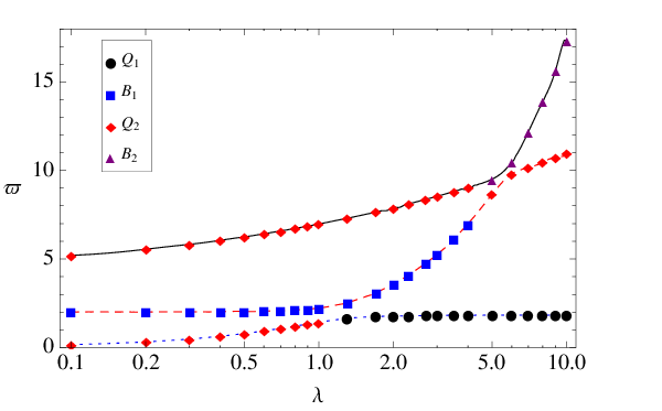
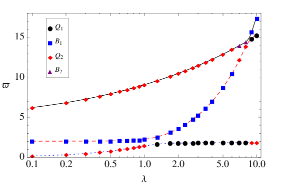
Figure 3: (Color online) Oscillation frequencies as a function of trap anisotropy in a condensate containing a singly (a) and doubly (b) charged vortex at its center. Solid (black) line is ϖξ\varpi_{\xi}, dashed (red) line is ϖρ\varpi_{\rho}, and dotted (blue) line is ϖz\varpi_{z}.
Refer to caption
(a) B1B_{1}
Refer to caption
(b) Q1Q_{1}
Refer to caption
(c) B2B_{2}
Refer to caption
(d) Q2Q_{2}
Figure 4: (Color online) Schematic representation of collective modes. B1B_{1} mode has all components oscillating in phase. B2B_{2} mode has rξr_{\xi} oscillating out of phase with rρr_{\rho} and rzr_{z}. Q1Q_{1} mode has rzr_{z} oscillation out of phase with rξr_{\xi} and rρr_{\rho}. Q2Q_{2} mode has rρr_{\rho} oscillation out of phase with rξr_{\xi} and rzr_{z}.

Since (58) is a cubic equation of ϖ2\varpi^{2}, we have three pair of frequencies ±ϖn\pm\varpi_{n} (n=z,ρ,ξn=z,\rho,\xi). There are three frequencies ϖn\varpi_{n} and four modes of oscillation in total, of which only three modes can be simultaneously observed depending on the anisotropy λ\lambda of harmonic potential as shown in fig.3. Among these four modes, two of them represent monopole oscillations while the other two represent quadrupole oscillations of the atomic cloud. The B1B_{1} mode (fig.4a) is characterized by having all condensate components rir_{i} (i=z,ρ,ξi=z,\rho,\xi) oscillating in phase, however B2B_{2} mode (fig.4c) presents rξr_{\xi} oscillating out of phase with rρr_{\rho} and rzr_{z}. The Q1Q_{1} mode (fig.4b) shows that rzr_{z} oscillation is out of phase with rξr_{\xi} and rρr_{\rho}, which are in phase with each other. However, in Q2Q_{2} mode (fig.4d) the oscillations of rzr_{z} and rξr_{\xi} are in phase with each other, being the rρr_{\rho} oscillation out of phase. Extrapolating to an ideal situation where γ=0\gamma=0, the equations of motions (37)–(39) can be decoupled. This way, the ϖz\varpi_{z} (lower frequency) represents only a rzr_{z} oscillation, ϖρ\varpi_{\rho} (middle frequency) represents only a rρr_{\rho} oscillation, and ϖξ\varpi_{\xi} (upper frequency) represents only a rξr_{\xi} oscillation.

Numerical simulations where performed in order to validate our results (fig.2). Frequency values ϖn\varpi_{n} in the variational calculations differ from numerical values by less than 1%.

In fig.3a, for 0.1≤λ≤10.1\leq\lambda\leq 1, exist two Q2Q_{2}-like modes. The difference between them comes from the fact that vortex core oscillation amplitude which is two orders of magnitude lower at the less energetic mode. The same happens when ℓ=2\ell=2 (fig.3b), i.e., the vortex core is almost still for the lower frequency in the same interval of λ\lambda.

The solid lines in fig.3 correspond to the mode with largest amplitude for the vortex-core oscillations. As can be seen, the excitation frequency ϖξ\varpi_{\xi} of this mode lowers as the vortex circulation increases. It means that the energy necessary to excite it will be lower if ℓ\ell is increased. However, we must point out that our results apply only for the cases where rξ≪rρr_{\xi}\ll r_{\rho}.

V Scattering length modulation

One of the mechanisms used for exciting collective modes is via modulation of the s-wave scattering length. This technique has been already applied to excite the lowest-lying quadrupole mode in a Lithium experiment [1]. Therefore, we consider the time-dependent scattering length:

as​(t)=a0+δ​a​cos⁡(Ω​t).a_{s}(t)=a_{0}+\delta a\cos\left(\Omega t\right). (59)

This is equivalent to make γ→γ⁡(τ)\gamma\rightarrow\gamma(\tau), thus giving:

γ⁡(τ)=γ0+δ​γ​cos⁡(Ω​τ).\gamma(\tau)=\gamma_{0}+\delta\gamma\cos\left(\Omega\tau\right). (60)

Where γ0\gamma_{0} is the average value of the interaction parameter γ⁡(τ)\gamma\left(\tau\right), δ​γ\delta\gamma is the modulation amplitude, and Ω\Omega is the excitation frequency. Substituting (60) into (57) and keeping only first-order terms (δ​ρ\delta\rho, δ​z\delta z, δ​α\delta\alpha, and δ​γ\delta\gamma), we obtain a nonhomogeneous linear equation

M​δ¨+V​δ=P​cos⁡(Ω​τ)M\ddot{\delta}+V\delta=P\cos\left(\Omega\tau\right) (61)

with

P=2​π​δ​γ​(2​D7rρ​03​rz​0D7rρ​02​rz​02D7′rρ​02​rz​0).P=2\pi\delta\gamma\begin{pmatrix}\frac{2D_{7}}{r_{\rho 0}^{3}r_{z0}}\\ \frac{D_{7}}{r_{\rho 0}^{2}r_{z0}^{2}}\\ \frac{D_{7}^{\prime}}{r_{\rho 0}^{2}r_{z0}}\end{pmatrix}. (62)

A particular solution of (61) is

δγ​(τ)=(M−1​V−Ω2)−1​M−1​P​cos⁡(Ω​τ).\delta_{\gamma}\left(\tau\right)=\left(M^{-1}V-\Omega^{2}\right)^{-1}M^{-1}P\cos\left(\Omega\tau\right). (63)

Projecting the vector δγ​(τ)\delta_{\gamma}\left(\tau\right) in the base δn\delta_{n} (n=z,ρ,ξn=z,\rho,\xi) of the eigenvectors of the homogenous equation associated to Eq.(61), we obtain

⟨δn|δγ​(τ)⟩=⟨δn|M−1​P⟩ϖn2−Ω2​cos⁡(Ω​τ).\left\langle\delta_{n}|\delta_{\gamma}\left(\tau\right)\right\rangle=\frac{\left\langle\delta_{n}|M^{-1}P\right\rangle}{\varpi_{n}^{2}-\Omega^{2}}\cos\left(\Omega\tau\right). (64)

Since |⟨δn|M−1​P⟩|>0\left|\left\langle\delta_{n}|M^{-1}P\right\rangle\right|>0 (fig.5), it shows that specific collective modes can be excited using a scattering length modulation with small amplitude δ​γ\delta\gamma and frequency Ω\Omega close to one of the resonance frequency ϖn\varpi_{n}. In fig.6, we see the results from a numerical solution of Eqs.(37)–(39) considering a time-dependent interaction γ⁡(τ)\gamma\left(\tau\right) according to Eq.(60). There we can see the beat behavior corresponding to a superposition of the frequencies Ω=6\Omega=6 and ϖξ=6.13\varpi_{\xi}=6.13.

Refer to caption
Figure 5: (Color online) Overlap between |M−1P⟩\left|M^{-1}P\right\rangle and normal modes |δn⟩\left|\delta_{n}\right\rangle as a function of the trap anisotropy with circulation ℓ=1\ell=1. The scalar product |⟨δn|M−1​P⟩|\left|\left\langle\delta_{n}|M^{-1}P\right\rangle\right| is always positive.
Refer to caption
(a)
Refer to caption
(b)
Refer to caption
(c)
Refer to caption
(d)
Figure 6: Numerical solution of Eqs.(37)–(39) with a time-dependent interaction γ⁡(τ)\gamma\left(\tau\right) (a, b, and c). (d) is the excitation spectrum obtained from variational calculation, where ϖξ≈6.13\varpi_{\xi}\approx 6.13 is close to the value calculated in Eq.(58). We excited the collective mode Q2Q_{2} (ϖξ=6.21\varpi_{\xi}=6.21) of a condensate with cigar shape (λ=0.1\lambda=0.1, γ0=800\gamma_{0}=800) via scattering modulation with amplitude δ​γ=0.4\delta\gamma=0.4 and frequency Ω=6\Omega=6.

VI Free expansion

Refer to caption
(a) ℓ=1\ell=1
Refer to caption
(b) ℓ=2\ell=2
Figure 7: (Color online) Ratio between vortex core size and radial cloud size for different trap anisotropies while in free expansion. The solid (black) line corresponds to a prolate condensate (λ=0.1\lambda=0.1), the dashed (blue) line to the isotropic case (λ=1\lambda=1), and the dotted (red) line to a oblate condensate (λ=8\lambda=8).

The time-of-flight pictures constitute the most common method to measure vortices in BEC. This method of switch off the magneto-optical trap and letting atomic cloud expand freely for some time, typically ten milliseconds and then taking a picture of the expanded cloud [5, 24, 25, 26, 27, 28]. For this purpose we use the equations of motion (37)–(39) without the terms arising from the harmonic potential, i.e.,

D1​rρ¨+G1​rρ​α¨+G2​rρ​α˙2+G3​rρ˙​α˙−G4rρ3−4​D7​γrρ3​rz\displaystyle D_{1}\ddot{r_{\rho}}+G_{1}r_{\rho}\ddot{\alpha}+G_{2}r_{\rho}\dot{\alpha}^{2}+G_{3}\dot{r_{\rho}}\dot{\alpha}-\frac{G_{4}}{r_{\rho}^{3}}-\frac{4D_{7}\gamma}{r_{\rho}^{3}r_{z}} =0,\displaystyle=0, (65)
D2​rz¨+G5​rz​α¨+G6​rz​α˙2+G7​rz˙​α˙−2​D7​γrρ2​rz2\displaystyle D_{2}\ddot{r_{z}}+G_{5}r_{z}\ddot{\alpha}+G_{6}r_{z}\dot{\alpha}^{2}+G_{7}\dot{r_{z}}\dot{\alpha}-\frac{2D_{7}\gamma}{r_{\rho}^{2}r_{z}^{2}} =0,\displaystyle=0, (66)
D1′​rρ​rρ¨+D2′​rz​rz¨+(G8​rρ2+G9​rz2)​α¨+(G10​rρ2+G11​rz2)​α˙2\displaystyle D_{1}^{\prime}r_{\rho}\ddot{r_{\rho}}+D_{2}^{\prime}r_{z}\ddot{r_{z}}+\left(G_{8}r_{\rho}^{2}+G_{9}r_{z}^{2}\right)\ddot{\alpha}+\left(G_{10}r_{\rho}^{2}+G_{11}r_{z}^{2}\right)\dot{\alpha}^{2}
+(G12​rρ​rρ˙+G13​rz​rz˙)​α˙+G14rρ3+4​D7′​γrρ2​rz\displaystyle+\left(G_{12}r_{\rho}\dot{r_{\rho}}+G_{13}r_{z}\dot{r_{z}}\right)\dot{\alpha}+\frac{G_{14}}{r_{\rho}^{3}}+\frac{4D_{7}^{\prime}\gamma}{r_{\rho}^{2}r_{z}} =0,\displaystyle=0, (67)

whose initial conditions are given by the stationary equations (54)–(56). This result agrees with our preview work [21], where the free expansion of the vortex core is given in fig.7. In [21], the fig.7b could not be calculated since the authors considered the healing length as an approximation to the vortex core radius which is only valid for ℓ=1\ell=1.

VII Conclusions

In this paper we proposed a modification in the wave function phase commonly used with the variational method which corrects the imaginary frequencies of collective modes when we have a parameter describing non-physical vortex core dynamics with ℓ=1\ell=1.

Here we consider variational phase parameters corresponding to each parameter in wave function amplitude, respectively. This way, we were able to describe the dynamics of both vortex core and the external dimensions of the condensate which agrees with the numerical simulations of the GPE. Although we observe four modes of oscillation in total, only three of them can be simultaneously observed depending on the trap anisotropy.

We also demonstrate that these oscillation modes can be excited by modulating the s-wave scattering length using the same experimental techniques as in Ref. [1].

Finally, we analyzed the time-of-flight dynamics of the vortex core with different circulations in order to complement the results in Ref. [21].

Acknowledgements.
We acknowledge the financial support of from the National Council for the Improvement of Higher Education (CAPES) and from the State of São Paulo Foundation for Research Support (FAPESP).

References

  • [1] S. E. Pollack, D. Dries, R. G. Hulet, K. M. F. Magalhães, E. A. L. Henn, E. R. F. Ramos, M. A. Caracanhas, and V. S. Bagnato, Physical Review A 81, 053627 (2010).
  • [2] S. Stringari, Physical Review Letters 77, 2360 (1996).
  • [3] V. M. Pérez-García, H. Michinel, J. I. Cirac, M. Lewenstein, and P. Zoller, Physical Review Letters 77, 5320 (1996).
  • [4] F. Dalfovo, S. Giorgini, L. P. Pitaevskii, and S. Stringari, Reviews of Modern Physics 71, 463 (1999).
  • [5] P. W. Courteille, V. S. Bagnato, and V. I. Yukalov, Laser Physics 11, 659 (2001).
  • [6] T. Busch, J. I. Cirac, V. M. Pérez-García, and P. Zoller, Physical Review A 56, 2978 (1997).
  • [7] Z. Zhang and W. V. Liu, Physical Review A 83, 023617 (2011).
  • [8] H. Heiselberg, Physical Review Letters 93, 040402 (2004).
  • [9] A. Altmeyer, S. Riedl, C. Kohstall, M. J. Wright, R. Geursen, M. Bartenstein, C. Chin, J. H. Denschlag, and R. Grimm, Physical Review Letters 98, 040401 (2007).
  • [10] M. Človečko, E. Gažo, M. Kupka, and P. Skyba, Physical Review Letters 100, 155301 (2008).
  • [11] C. J. Pethick and H. Smith, Bose-einstein condensation in dilute gases (Cambridge University Press, Cambridge, 2008), 2nd ed.
  • [12] L. P. Pitaevskii and S. Stringari, Bose-Einstein Condensation (Oxford University Press Inc, 2003), first edition ed.
  • [13] A. A. Svidzinsky and A. L. Fetter, Physical Review A 62, 063617 (2000a).
  • [14] A. A. Svidzinsky and A. L. Fetter, Physical Review Letters 84, 5919 (2000b).
  • [15] M. Linn and A. L. Fetter, Physical Review A 61, 063603 (2000).
  • [16] V. M. Pérez-García and J. J. García-Ripoll, Physical Review A 62, 033601 (2000).
  • [17] V. M. Pérez-García, H. Michinel, J. I. Cirac, M. Lewenstein, and P. Zoller, Physical Review A 56, 1424 (1997).
  • [18] A. A. Svidzinsky and A. L. Fetter, Physical Review A 58, 3168 (1998).
  • [19] D. H. J. O’Dell and C. Eberlein, Physical Review A 75, 013604 (2007).
  • [20] F. Dalfovo and M. Modugno, Physical Review A 61, 023605 (2000).
  • [21] R. P. Teles, F. E. A. dos Santos, M. A. Caracanhas, and V. S. Bagnato, Physical Review A 87, 033622 (2013).
  • [22] E. A. de Lima Henn, Ph.D. thesis, Instituto de Física de São Carlos, Universidade de São Paulo, São Carlos (2008).
  • [23] G. R. Dennis, J. J. Hope, and M. T. Johnsson, Computer Physics Communications 184, 201 (2013).
  • [24] W. Ketterle, MIT Physics Annual pp. 44–49 (2001).
  • [25] E. A. L. Henn, J. A. Seman, E. R. F. Ramos, M. Caracanhas, P. Castilho, E. P. Olímpio, G. Roati, D. V. Magalhães, K. M. F. Magalhães, and V. S. Bagnato, Physical Review A 79, 043618 (2009a).
  • [26] E. A. L. Henn, J. A. Seman, G. Roati, K. M. F. Magalhães, and V. S. Bagnato, Physical Review Letters 103, 045301 (2009b).
  • [27] F. Chevy, K. W. Madison, and J. Dalibard, Physical Review Letters 85, 2223 (2002).
  • [28] B. P. Anderson and P. C. Haljan, Physical Review Letters 85, 2857 (2000).