Metric Dimension for Gabriel Unit Disk Graphs is NP-Complete
Abstract
We show that finding a minimal number of landmark nodes for a unique virtual addressing by hop-distances in wireless ad-hoc sensor networks is NP-complete even if the networks are unit disk graphs that contain only Gabriel edges. This problem is equivalent to Metric Dimension for Gabriel unit disk graphs. The Gabriel edges of a unit disc graph induce a planar distance and an optimal energy spanner. This is one of the most interesting restrictions of Metric Dimension in the context of wireless multi-hop networks.
Keywords:
metric dimension , unit disk graph , gabriel graph , virtual address , wireless multi-hop network , sensor network1 Introduction
Wireless radio networks in which all nodes have the same radio range are often modeled as unit disc graphs. An undirected graph is a unit disk graph (UDG) if its vertices can be embedded in the Euclidean plane by an embedding such that two vertices are connected by an edge if and only if their Euclidean distance is at most . The vertices represent the sensor nodes and the undirected edges the symmetric communication channels between them. Two sensor nodes can communicate with each other, if they are close enough.
A widely used idea to reduce the complexity of distributed algorithms for wireless ad-hoc sensor networks is to consider only some of the available connections. The strongest restriction that preserves connectivity is a spanning tree. A spanning tree unfortunately does not allow efficient routing through the network. A slightly weaker restriction is the Gabriel graph [13]. An edge of an embedded graph is a Gabriel edge, if there is no vertex such that . The Gabriel edges induce a planar distance and optimal energy spanner of , see [3]. That is, the ratio between the length of a shortest path in and is of if the costs of the edges are , and if the costs of the edges are for some .
Many routing algorithms for wireless ad-hoc sensor networks are based on virtual coordinates, see for example VCap [5], JUMPS [2], GLIDER [11], VCost [10], BVR [12], and HBR [15]. The virtual coordinates are computed from the distances to specific nodes called landmarks, anchors, or beacons [12, 18]. The setup of the virtual addressing starts by selecting some landmark nodes that flood large parts of the network. After that every node defines its virtual coordinates depending on the distances to the landmark nodes.
The virtual coordinates can be used to route a message through the network. Most routing algorithms require the virtual addresses to be unique. Packet delivery is also only guaranteed if different nodes have different virtual coordinates. The length of the virtual addresses increases with the number of landmark nodes. Since every landmark node has to flood large parts of the network during initialization, the number of landmark nodes should be as small as possible to reduce the amount of consumed energy. These conditions cause the question of how to determine a minimum set of landmark nodes that provides a unique virtual addressing.
From a graph theoretical point of view, the decision version of the problem above is called Metric Dimension. A set of vertices of a graph is called a resolving set, if for every vertex pair there is at least one vertex such that the distance between and differs from the distance between and . A graph has metric dimension at most if there is a resolving set of size at most . Metric Dimension is known to be NP-complete for general graphs as well as for planar graphs [9, 14, 18]. For a fixed number of landmarks it is decidable in polynomial time. It is also decidable in polynomial time for special classes of graphs like trees, wheels, complete graphs, -regular bipartite graphs and outerplanar graphs [7, 9, 18, 19, 20]. The approximability of Metric Dimension by centralized algorithms has been studied for bounded degree, dense, and general graphs in [16]. There are also boundaries for the metric dimension of some special classes of graphs, see [6, 8].
In this paper, we prove that Metric Dimension is NP-complete even for unit disk graphs that contain only Gabriel edges. This is the most interesting restriction of the problem in the context of computing unique virtual addresses in wireless ad-hoc sensor networks. We show how to construct in polynomial time for an arbitrary instance of a special satisfiability problem a Gabriel unit disk graph and an integer such that there is a satisfying truth assignment for if and only if there is a resolving set for of size at most .
2 Definitions and terminology
Let be a directed or undirected graph. That is, is the set of vertices and is the set of directed edges or undirected edges , respectively. A graph is a subgraph of if and . It is an induced subgraph of if or , respectively.
A sequence of vertices of is called a directed path if is directed and for . It is called an undirected path if is undirected and for .
2.1 Gabriel unit disk graphs
For a vector , let be its Euclidean norm.
Definition 1
An undirected graph is a unit disk graph (UDG) if there is a UDG embedding such that , and .
Definition 2
For an undirected graph and an embedding of its vertices an edge is a Gabriel edge if there is no vertex with
An undirected graph is a Gabriel UDG (GUDG) if there is a UDG embedding for which all edges in are Gabriel edges. Such an embedding is called a GUDG embedding.
Definition 3
A graph is planar if there is an embedding with the following two properties:
- 1.
, and
- 2.
for every edge between two vertices and there is a line in connecting the points and such that no two lines for two different edges intersect except at a common endpoint.
2.2 Metric Dimension
The distance between two nodes in a graph is the smallest integer for which there is a path between and with edges.
Definition 4
In this paper, we consider the complexity of the following decision problem.
GUDG Metric Dimension
| Given: | A GUDG and a positive integer . |
|---|---|
| Question: | Is there a resolving set for of size at most ? |
2.3 Satisfiability
Let be a set of boolean variables. A truth assignment for is a function . If then we say variable is true under ; if then we say variable is false under . If is a variable of then and are literals over ; is called a positive literal, is called a negative literal. The positive literal is true under if and only if variable is true under ; negative literal is true under if and only if variable is false under . A clause over is a set of literals over . It represents the disjunction of literals which is satisfied by a truth assignment if and only if at least one of its literals is true under . A collection of clauses over is satisfiable if and only if there is a truth assignment that simultaneously satisfies all clauses of .
Definition 5
Let be a set of boolean variables and be a collection of clauses over . The directed clause variable graph of has a vertex for every variable and a vertex for every clause . There is a directed edge from variable vertex to clause vertex if and only if contains literal or .
The following problem is NP-complete as shown in Corollary 3 of [9].
-Negative Planar 3-Sat
| Given: | A set of boolean variables and a collection of clauses over such that • every variable occurs in exactly two or three clauses, once as a negative literal, and once or twice as a positive literal, • the clause variable graph for is planar, • every clause contains two or three literals and • every clause with three literals contains at least one negative literal. |
|---|---|
| Question: | Is there a satisfying truth assignment for ? |
Definition 6
Let be a directed planar graph and be an embedding of the vertices of . An edge path of length for an edge is a sequence of points for which
- 1.
,
- 2.
, , and
- 3.
for , if then
.
A planar orthogonal grid drawing of a directed graph is a pair where
- •
is an embedding of the vertices of ,
- •
is a collection of edge paths, one for every edge of , and
- •
no two distinct edge paths and of have a common point unless the corresponding two edges and have a common vertex and .
3 Main result
Theorem 1
GUDG Metric Dimension is NP-complete.
The membership to NP is obvious, because it is easy to verify in polynomial time whether a given set of vertices is a resolving set. The NP-hardness is shown by a reduction from -Negative Planar 3-Sat.Every directed planar graph with vertex degree at most four has a planar orthogonal grid drawing, whose size (determined by the number of grid points used for the edge paths) is polynomially bounded in the number of vertices. Such a drawing can be computed in polynomial time using the algorithms described in [21, 22]. Let be a planar clause variable graph for . Since the vertices of have a degree of at most three, we can assume that we have a planar orthogonal grid drawing for .
The following preprocessing phase modifies into an equivalent instance for which there is a planar orthogonal grid drawing for the clause variable graph whose edge paths have a length of at most two. This upper bound on the length of the edge paths is necessary, because the gadget that is going to represent the edge paths cannot be embedded across arbitrarily large areas.
Let be an edge of the clause variable graph whose edge path in is with length . Assume clause contains a positive literal (the case for a negative literal runs analogously). Then a new variable and a new clause are inserted and the positive literal in clause is replaced by the positive literal . The new sets of variables and clauses again define an instance for -Negative Planar 3-Sat that has a satisfying truth assignment if and only if the original instance has a satisfying truth assignment. The original planar orthogonal grid drawing for is modified for the new clause variable graph as follows. Define , , , , and . The old edge path of length is now replaced by two edge paths of length and one edge path of length . This splitting step is repeated until all edge paths have length at most two. See Figure 1 for an example.

3.1 The construction of
The GUDG is assembled using copies of the following 6 graphs called gadgets. Some of these gadgets are similar to the gadgets used in [9] for the proof that Planar Metric Dimension is NP-complete. The modifications are done to obtain GUDGs. Every gadget has two or three special path pairs called -path pairs. The -path pairs are used to represent the edges of the clause variable graph . The end-vertices of degree one of a -path pair are called a -vertex pair.
- 1.
There are three variable gadgets , and for the variables of , see Figure 2. The first variable gadget is used for the case that the corresponding variable is contained in three clauses, once as a negative literal and twice as a positive literal. The other two are used for the case that the corresponding variable is contained in two clauses, once as a negative literal and once as a positive literal.
These three gadgets have two different types of -path pairs marked by for the negative literal and for the positive literals. The --vertex pair is , the --vertex pairs are and .
- 2.
There are two clause gadgets for the clauses of , see Figure 3 to the left and in the middle. The first clause gadget is used for clauses with three literals. The second clause gadget is an induced subgraph of . It is used for clauses with two literals.
The -vertex pairs are , and .
- 3.
There is an edge gadget for the edges of , see Figure 3 to the right. It is used to connect variable gadgets with clause gadgets and consists of two disjoint paths with 37 vertices each.
These two paths represent one -path pair with two -vertex pairs and .


Graph contains for every variable with two positive literals and one negative literal in the clauses of a copy of . It contains for every variable with one positive and one negative literal in the clauses of a copy of or . Then contains for every clause of with three literals one copy of and for every clause of with two literals one copy of . Finally it contains for every edge of one copy of .
The gadgets are connected to each other by identifying -vertex pairs as follows. Let be a variable gadget for variable , a clause gadget for clause , and the edge gadget for the edge . One -vertex pair of is identified with one -vertex pair of and the other -vertex pair of is identified with one -vertex pair of . If clause contains the positive literal , then a --vertex pair is used, otherwise, a --vertex pair is used.
Identifying two -vertex pairs and means that all vertices adjacent to are connected to , all vertices adjacent to are connected to , and then the two vertices and their incident edges are removed.
3.2 A GUDG embedding for
In this section, it is shown that can be assembled such that there is a GUDG embedding for . For each gadget we present several different GUDG embeddings. In every of these embeddings the vertices of the gadget are mapped to positions inside a polygon. The -vertices are placed at the border of the polygon. The non--vertices, i.e. all vertices not belonging to a -vertex pair, are placed at positions with a distance to all positions outside the polygon.
Definition 7
A tile is a pair , where is one of the gadgets defined above and is a GUDG embedding for , called tile embedding, such that for every -vertex pair ,
The -vertices are placed at the border of the square with side length and center .
All other vertices of the gadget are mapped to positions of the square that have a distance to all positions of outside the square .
We consider several different tile embeddings for gadget . These are the three tile embeddings shown in Figure 4 and all tile embeddings obtained by , , or degree rotations and/or a horizontal or vertical mirroring. The rotations by , , and degree and the horizontal and vertical mirroring can be performed by the mappings


We also consider several different tile embeddings for every gadget , , , , and , see Figures 5, 6, and 7.


The tile embeddings resulting from the last embedding of Figure 7 for edge gadget are only used for edges whose edge paths have length 1. For edge paths of length 2, the following definition is used.
Let be the square of side length and center translated by . The vertices of are mapped to positions of one of the following polygons , , formed by the union of squares.


Definition 8
A tile triple is a pair , where is the edge gadget defined above and for some is a GUDG embedding for , called tile triple embedding, such that is either ,
,
,
,
,
or , respectively.
Every non--vertex is mapped to a position of with a distance to all positions outside of .


Definition 9
The orientation of a -vertex pair inside a tile (triple) is TF, if is encounter before on a clockwise traversal of the corresponding polygon and FT otherwise.
Definition 10
The connection vector of a tile is a -tuple consisting of components , where is the orientation of the -vertex pair on the -th side of the square
or , if none exists. The sides of the square are enumerated clockwise, starting from the top. If is a variable gadget and , then denotes whether is an --vertex pair or an --vertex pair. For all other cases set .
Now define the equivalence relation on the space of connection vectors as follows:
if and only if there exists a , such that for all , . The type of a tile is the equivalence class of its connection vector, denoted by one representative in square brackets. Table 1 lists the types of all available tile embeddings.
type gadget tile embedding fig.4 () fig.4 (), mirrored fig.4 () fig.4 (), mirrored fig.4 () fig.4 (), mirrored fig.5 () fig.5 (), mirrored fig.5 () fig.5 (), mirrored fig.5 () fig.5 (), mirrored fig.6 () fig.6 (), mirrored fig.6 () fig.6 (), mirrored fig.6 () fig.6 (), mirrored fig.7 () fig.7 (), mirrored fig.7 () fig.7 () fig.7 (), mirrored fig.7 () fig.7 (), mirrored fig.7 ()
Next we place the tiles and tile triples according to the planar orthogonal grid drawing of the clause variable graph .
Let be an edge of with edge path . Edge is from-left, from-right, from-top, or from-bottom if , , , or , respectively. Analogously it is to-left, to-right, to-top, or to-bottom if , , , or . Edge is a -edge or a -edge if variable occurs in clause as a positive or negative literal.
A tile or tile triple has a left-, right-, top-, or bottom--vertex pair if gadget has a -vertex pair mapped to such that , , , or , respectively.
Let be a variable vertex of and be the copy of the gadget for . Then a tile for is chosen whose -vertices are arranged according to the directions of the edges from in the following sense. If, for example, is a -from-left edge then tile has a right---vertex pair. If is a -from-top edge then tile has a bottom---vertex pair, etc.
Let be a clause vertex of and be the copy of the gadget for . Then a tile for is chosen whose -vertices are arranged according to the directions of the edges to in the following sense. If, for example, is a to-left edge then tile has a right--vertex pair. If is a to-top edge then tile has a bottom--vertex pair, etc.
Let be an edge of and be the copy of the gadget for . Then a tile or tile triple for is chosen whose -vertices are arranged according to the direction of edge in the following sense. If, for example, is a from-left-to-right edge then has a left- and a right--vertex pair. If is a from-top-to-bottom edge then has a top- and bottom--vertex pair, etc.
To construct a GUDG embedding for we place the vertices of the gadgets as follows.
- 1.
Let be a gadget inserted into for a variable or clause vertex of the clause variable graph , and let be the selected tile. Then the GUDG embedding for the vertices from gadget is defined by .
- 2.
Let be a gadget inserted into for an edge path
of length , and let be the selected tile for gadget . Then the GUDG embedding for the vertices from gadget is defined by . - 3.
Let be a gadget inserted into for an edge path
of length , and let be the selected tile triple for gadget . Then the GUDG embedding for the vertices from gadget is defined by .
Figure 9 shows an example of the placed tiles for the clause variable graph of Figure 1.
Graph is defined by the union of gadgets through identification of their -vertices. Thus we have to show that it is always possible to select a tile (or tile triple) for every inserted copy of a gadget such that identified vertices are placed at the same position.
Every tile and tile triple embedding is a GUDG embedding. A GUDG embedding for the inner part used in the variable gadgets is shown in Figure 9. The distance between non--vertices from different tiles is always greater than . Thus, the resulting embedding is a GUDG embedding for .


If is identified with and is identified with then there only are the following two cases left to be considered due to the restrictions for the placement of -vertex pairs inside tiles and tile triples. Either or . In the first case there is no problem, the second case is called an orientation conflict. is a valid embedding if it has no orientation conflicts.
Lemma 1
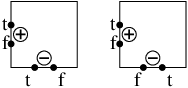
Let be a variable tile. Then there also is a variable tile with:
- 1.
- 2.
for all --vertex pairs in there is a --vertex pair in
such that .

Lemma 2
Let be a clause tile and , two distinct -vertex pairs in . Then there also are three other tiles , and with:
-
,
-
,
-
,
Lemmata 1 and 2 can easily be verified using table 1. Note that the tile in Lemma 1 may contain a different variable gadget. This is the case for a variable that occurs only once as a positive literal.
Theorem 2
is a GUDG if the correct gadgets for all variables are chosen during the assembly. The assembly can be computed in polynomial time.
Proof 1
The only ambiguity during the assembly of is the selection of either or for a variable that occurs once as a positive literal. To decide which gadget has to be used, we start with any selection of tiles for the variable and clause vertices that fit the directions of the edges of as described above. By selecting tiles and tile triples for the edge gadgets that do not cause an orientation conflict with the adjacent variable tile, we can assume w.l.o.g. that all orientation conflicts are directly between clause and variable tiles. Now resolve all existing orientation conflicts as follows: By Lemma 2 we can select a clause tile for every clause containing two literals that does not cause any orientation conflicts with the adjacent two variable tiles. For every clause containing three literals we can select a clause tile that causes at most one orientation conflict. Since every clause with three literals contains at least one negative literal we can restrict this orientation conflict to the variable tile for variable . By Lemma 1, we can then select a variable tile that causes neither this orientation conflict nor one with another adjacent clause tile. is the variable gadget that has to be used for variable during the assembly of . Since every orientation conflict is solved by at most three local replacements of tiles and tile triples that never cause new orientation conflicts to appear the tile selection for a valid GUDG embedding, and by extend the GUDG , can be computed in polynomial time.
3.3 Correctness
In this section, we prove that there is a resolving set for of size at most if and only if there is a satisfying truth assignment for .
Definition 11
Let be an undirected graph. A vertex resolves a vertex pair if . A vertex pair is called unsolved by set , if no vertex of resolves .
Lemma 3
Every resolving set for contains at least three vertices of each copy of a variable gadget . contains vertex or for , see Figure 2.
Proof 2
Suppose neither nor is in for some . Since all shortest paths from any vertex of to and contain and , there is no vertex that resolves the pair .
Let be a set of vertices consisting of one vertex from , , for every copy of a variable gadget, i.e., . The vertices in are called forced landmarks.
Lemma 4
Every vertex pair and from the same copy of a variable gadget and every vertex pair from the same copy of a clause gadget are unsolved by . For all other vertex pairs , there is a forced landmark of that resolves .
Proof 3
Let be an arbitrary vertex pair of .
Case 1
and belong to the same gadget copy .
Case 1.1
is a variable gadget copy. Vertex pair is unsolved by , because every shortest path from a landmark of to and passes one of the vertices and for . Analogously, vertex pair is unsolved by , since for . The vertex pairs , , are resolved by the forced landmarks from the variable gadgets connected to this -path pair via one clause gadget and two edge gadgets. All other vertex pairs are resolved by one of the forced landmarks of , see table 2.
Case 1.2
is an edge gadget copy. All edge gadgets are basically extensions of the -path pairs inside the clause and variable gadgets, so this case has already been covered in case 1.1.
Case 1.3
is a clause gadget copy. The vertex pair is unsolved by , because all shortest paths from the forced landmarks to and enter via an path and pass vertex . All other vertex pairs are resolved by at least one forced landmark in an adjacent variable gadget copy, see table 3.
Case 2
and belong to different gadget copies.
Case 2.1
and belong to variable gadget copies and , respectively. All forced landmarks of resolve the pair : The distance from a forced landmark of to any vertex of is at most (e.g. ) while the distance to any vertex of is greater than , because any shortest path has to traverse at least two edge gadgets and one clause gadget.
Case 2.2
and both belong to edge gadget copies. Let and be the forced landmarks closest to and , respectively. Also for all forced landmarks , because all vertices at distance from are either in a clause gadget, an edge gadget or the variable gadget that belongs to, hence none of them being another forced landmark. Now suppose that neither nor resolves the pair , meaning and . Together we get , which contradicts to the assumption that is the landmark closest to .
Case 2.3
and belong to the clause gadget copies and for the clauses and , respectively.
Case 2.3.1
There is a variable such that contains literal or and does contain neither nor . The forced landmarks of variable gadget for resolve the pair : All shortest paths from forced landmarks of to vertices of the adjacent clause gadget have a length of at most (e.g. ), while all shortest paths to vertices of a non-adjacent clause gadget have a length greater than , since they have to traverse three edge gadgets, one clause gadget and one variable gadget.
Case 2.3.2
All variables that occur as a literal in also occur as a literal in and vice versa. Since there is one variable such that and or and . W.l.o.g. let , . Furthermore let and be the forced landmarks in closest to and , respectively. Then and . Now assume is unsolved by . Then and . Together we get which is a contradiction.
Case 2.4
belongs to variable gadget copy and to edge gadget copy .
Case 2.4.1
is adjacent to . See case 1.1.
Case 2.4.2
is not adjacent to . Every forced landmarks in resolves : The distance from to any vertex in is at most while the distance to any vertex in is greater than , since the shortest path has to traverse at least one other edge gadget and one clause gadget.
Case 2.5
belongs to variable gadget copy and to clause gadget copy . See case 2.4.2.
Case 2.6
belongs to clause gadget copy and to edge gadget copy .
Case 2.6.1
is adjacent to . See case 1.3.
Case 2.6.2
is not adjacent to . If belongs to a -vertex pair of then this case has already been covered in one of the previous cases, because has been identified with a vertex from a clause or variable gadget. So we can assume that . Let be the forced landmark closest to inside a variable gadget adjacent to . Then resolves , because while the distance from to any vertex in is at least .
Lemma 5
The vertex pair can only be resolved by , , , or of the same gadget copy .
Proof 4
Anyone of these vertices obviously resolves and except for they also resolve . Furthermore there are shortest paths from and to any other vertex in that cross either or , meaning that does not resolve , because .
Theorem 3
GUDG Metric Dimension is NP-complete.
Proof 5
Let be an instance for -Negative Planar 3-Sat and , the instance for GUDG Metric Dimension as described above. Then is satisfiable resolving set .
: Because is satisfiable, the altered instance with variable set and clause set is also satisfiable. Let be a satisfying truth assignment for . For every variable choose of the corresponding variable gadget copy as a landmark if and otherwise. Together with this set of vertices is a resolving set: According to Lemmata 4 and 5 all pairs are resolved except for of each clause gadget copy. Since satisfies each clause gadget copy is connected to either the --path pair of a variable gadget copy in which has been chosen as a landmark or to one of the --path pairs of a variable gadget copy in which has been chosen as a landmark. In both cases, for some , the shortest path from this landmark to enters the clause gadget through the path while the shortest path to enters the gadget through the path, thus resolving .
: Let be a resolving set for with vertices. According to Lemmata 3 and 5 contains forced landmarks and one of the vertices , , , or for every variable in . Now construct a truth assignment for by setting to if the fourth landmark in ’s variable gadget copy is and otherwise. Then satisfies : resolves in every clause gadget copy, so there is one landmark for each copy such that . This implies that the shortest path from to either or does not contain and enters the clause gadget through the adjacent path. So has to be inside the variable gadget that is connected to the clause gadget through one edge gadget:
Assume that it is not. Then has to traverse an entire clause gadget and another variable gadget first. Independent of where enters , on a shortest path to a vertex outside of it is never shorter to leave through a path than crossing ’s node and leaving through the path. So enters through an path, maybe contains the node of and leaves through another path, hence not resolving .
Since enters the clause gadget through the path and also resolves in its variable gadget, has been set to if the clause gadget is connected to the --path pair of the variable gadget and otherwise. So every clause contains at least one positive literal whose variable is set to or one negative literal whose variable is set to , meaning that is satisfied. And because is satisfiable, the original instance is satisfiable.
References
- [1] INFOCOM 2005. 24th Annual Joint Conference of the IEEE Computer and Communications Societies, 13-17 March 2005, Miami, FL, USA. IEEE, 2005.
- [2] F Benbadis, J.-J. Puig, M. Dias de Amorim, C. Chaudet, T. Friedman, and D. Simplot-Ryl. Jumps: Enhancing hop-count positioning in sensor networks using multiple coordinates. CoRR, abs/cs/0604105, 2006.
- [3] P. Bose, L. Devroye, W.S. Evans, and D.G. Kirkpatrick. On the spanning ratio of gabriel graphs and -skeletons. SIAM Journal on Discrete Mathematics, 20(2):412–427, 2006.
- [4] D.L. Boutin. Determining sets, resolving sets, and the exchange property. Graphs and Combinatorics, 25(6):789–806, 2009.
- [5] A. Caruso, S. Chessa, S. De, and A. Urpi. Gps free coordinate assignment and routing in wireless sensor networks. In INFOCOM [1], pages 150–160.
- [6] G.G. Chappell, J.G. Gimbel, and C. Hartman. Bounds on the metric and partition dimensions of a graph. Ars Comb., 88, 2008.
- [7] G. Chartrand, L. Eroh, M.A. Johnson, and O. Oellermann. Resolvability in graphs and the metric dimension of a graph. Discrete Applied Mathematics, 105(1-3):99–113, 2000.
- [8] G. Chartrand, C. Poisson, and P. Zhang. Resolvability and the upper dimension of graphs. Computers and Mathematics with Applications, 39(12):19–28, 2000.
- [9] J. Diaz, O.M. Pottonen, M. Serna, and E.J. van Leeuwen. On the complexity of metric dimension. In Algorithms â ESA 2012, volume 7501 of Lecture Notes in Computer Science, pages 419–430. Springer Berlin Heidelberg, 2012.
- [10] E. H. Elhafsi, N. Mitton, and D. Simplot-Ryl. Cost over progress based energy efficient routing over virtual coordinates in wireless sensor networks. In WOWMOM, pages 1–6. IEEE, 2007.
- [11] Q. Fang, J. Gao, L.J. Guibas, V. de Silva, and L. Zhang. GLIDER: gradient landmark-based distributed routing for sensor networks. In INFOCOM [1], pages 339–350.
- [12] R. Fonseca, S. Ratnasamy, J. Zhao, C.T. Ee, D.E. Culler, S. Shenker, and I. Stoica. Beacon vector routing: Scalable point-to-point routing in wireless sensornets. In NSDI. USENIX, 2005.
- [13] R.K. Gabriel and R.R. Sokal. A new statistical approach to geographic variation analysis. Systematic Zoology, 18(3):259–278, 1969.
- [14] M.R. Garey and D.S. Johnson. Computers and Intractability: A Guide to the Theory of NP-Completeness. W.H. Freeman, 1979.
- [15] D. Gaußmann, S. Hoffmann, and E. Wanke. Hierarchical bipartition routing for delivery guarantee in sparse wireless ad hoc sensor networks with obstacles. In ICWN, pages 3–9. CSREA Press, 2012.
- [16] M. Hauptmann, R. Schmied, and C. Viehmann. On approximation complexity of metric dimension problem. In Proceedings of the 21st international conference on Combinatorial algorithms, IWOCA’10, pages 136–139, Berlin, Heidelberg, 2011. Springer-Verlag.
- [17] M.C. Hernando, M. Mora, I.M. Pelayo, C. Seara, J. Cáceres, and M.L. Puertas. On the metric dimension of some families of graphs. Electronic Notes in Discrete Mathematics, 22:129–133, 2005.
- [18] S. Khuller, B. Raghavachari, and A. Rosenfeld. Landmarks in graphs. Discrete Applied Mathematics, 70(3):217–229, 1996.
- [19] S.W. Saputro, E.T. Baskoro, A.N.M. Salman, D. Suprijanto, and A.M. Baca. The metric dimension of regular bipartite graphs. arXiv/1101.3624, 2011.
- [20] B. Shanmukha, B. Sooryanarayana, and K.S. Harinath. Metric dimension of wheels. Far East Journal of Applied Mathematics, 8(3):217–229, 2002.
- [21] R. Tamassia. On embedding a graph in the grid with the minimum number of bends. SIAM Journal on Computing, 16(3):421–444, 1987.
- [22] R. Tamassia and I.G. Tollis. Planar grid embedding in linear time. IEEE Transactions on Circuits and Systems, 36(9):1230–1234, 1989.