Zeno dynamics in quantum open systems

We define the projective measurement applied in the quantum Zeno dynamics as $\mathcal{P}[\circ]=M\circ M$ with $M=|\psi_{0}\rangle_{S}\langle\psi_{0}|$. A sequence of $m$ observations can repeatedly bring the system to the initial state with survival probability $P(t)=\textrm{Tr}\left(\mathcal{V}(\tau)^{m}[\rho_{S}(0)]\right)$, in which we define that $\mathcal{V}(\tau)=\mathcal{P}\mathcal{U}(\tau)\mathcal{P}$ and the interval is $\tau=t/m$. For the case of small time intervals $\tau\ll t$ with a large enough number of trials $m\rightarrow\infty$, the survival probability can be expanded in terms of intervals $\tau$ as

where

is called the dissipative Fisher information (d-FI)[23] because $\mathcal{F}^{\textrm{d}}\simeq{[\partial_{\tau}P(\tau)]^{2}}/\{P(\tau)[1-P(\tau)]\}$. Here, $\textrm{Cov}_{\rho}(X,Y)\equiv\textrm{Tr}(XY\rho)-\textrm{Tr}(X\rho)\textrm{Tr}(Y\rho)$ is the covariance of observables $X$ and $Y$ with respect to the state $\rho$ and $(\Delta X)^{2}=\textrm{Cov}_{\rho}(X,X)$ denotes the variance. The first term of $\mathcal{F}^{\textrm{d}}$ represents the contribution from the system and the second term represents that from the dissipative bath. $\tau_{Z}^{\textrm{d}}=2/\sqrt{m\mathcal{F}^{\textrm{d}}}$ is called as the dissipative quantum Zeno time (d-ZT) which coincides with the largest interval such that the two states remain indistinguishable[17]. We can conclude that the larger d-FI is, the shorter d-ZT will be and the harder quantum Zeno dynamics is to be realized.

Then, we consider an exactly solvable model, the damped Jaynes-Cummings model (JCM)[22], to study the Zeno dynamics in non-Markovian environments. A Hamiltonian of the total system is given by $H_{\textrm{tot}}=H_{S}+H_{B}+H_{I}$ where the system’s Hamiltonian is $H_{S}=\omega_{0}\sigma_{+}\sigma_{-}$, the Hamiltonian of vacuum reservoir is $H_{B}=\sum_{k}\omega_{k}b_{k}^{{\dagger}}b_{k}$, and $H_{I}=\sigma_{+}B+\sigma_{-}B^{{\dagger}}$ denotes the interaction Hamiltonian given that $B=\sum_{k}g_{k}b_{k}$ with $b_{k}$ ($b_{k}^{\dagger}$) the boson annihilation (creation) operator for the $k$th mode. Here, $\omega_{0}$ denotes the transition frequency of the atom with ground state $|0\rangle$ and excited state states $|1\rangle$; $\sigma_{x,y,z}$ are Pauli operators and $\sigma_{\pm}$ are the raising and lowering operators. The initial state is given as $|\psi_{0}\rangle=(|0\rangle+|1\rangle)/\sqrt{2}$. Given the Lorentzian spectral density $J(\omega)={\lambda W^{2}}/\{{\pi[(\omega-\omega_{0})^{2}+\lambda^{2}]}\}$ with $W$ the transition strength and $\lambda$ the spectral width of the coupling, we can obtain the master equation $\dot{\rho}^{I}_{S}(t)=\gamma(t)[\sigma_{-}\rho_{S}^{I}(t)\sigma_{+}-\frac{1}{2}\{\sigma_{+}\sigma_{-},\rho_{S}^{I}(t)\}]$ where the time-dependent decay rate $\gamma(t)$ is written in two conditional forms:

with $d=\sqrt{|\lambda^{2}-4W^{2}|}$. In the weak coupling regime $W<\lambda/2$, $\gamma(t)$ is always positive which corresponds to the Markovian process, while in the strong coupling regime $W\geq\lambda/2$, the function $\gamma(t)$ becomes negative within certain intervals of time, which displays the non-Markovianity[24]. For both Markovian and non-Markovian regimes, we obtain the same results as $\dot{\gamma}(0)=4W^{2}$. The d-FI is calculated as $\mathcal{F}^{\textrm{d}}=\omega_{0}^{2}+W^{2}$ which leads to $\tau_{Z}^{\textrm{d}}=2/\sqrt{m(\omega_{0}^{2}+W^{2})}$. If there is no noise $W=0$, the result will reduce to the unitary evolution case as discussed in Ref. [17]. When the transition strength becomes larger, d-FI grows and d-ZT decreases, which makes the Zeno dynamics more difficult. Moreover, given a definite value of transition strength $W$, d-FI is independent of $\lambda$ and the result stays unchanged for both Markovian and non-Markovian noise. The interpretation of this extraordinary result may be that in this example the initial dynamics characteristics of the open system do not depend on Markovianity or non-Markovianity.

Next, for the same initial state, we consider another exactly solvable model, the independent boson model, with $H_{S}=\omega_{0}\sigma_{z}/2$, $H_{B}=\sum_{k}\omega_{k}b_{k}^{{\dagger}}b_{k}$ and $H_{I}=\sum_{k}\sigma_{z}(g_{k}b_{k}^{{\dagger}}+g_{k}^{*}b_{k})$. We consider the general Ohmic-like spectral density with exponential cutoff $J(\omega)=\alpha\omega_{c}^{1-s}\omega^{s}e^{-\omega/\omega_{c}}$: for $s=1$ it is Ohmic; for $s>1$ it is super-Ohmic; for $s<1$ it is sub-Ohmic[22]. The bath is assumed to be initially in a thermal state: $\rho_{B}=\exp(-H_{B}/T)/\textrm{Tr}[{\exp(-H_{B}/T)}]$ given $T$ the temperature. Then we can obtain the master equation as $\dot{\rho}^{I}_{S}(t)=\gamma(t)\left[\sigma_{z}\rho_{S}^{I}(t)\sigma_{z}-\rho_{S}^{I}(t)\right]$ where $\gamma(t)=2\int_{0}^{\infty}d\omega J(\omega)\coth\left(\frac{\omega}{2T}\right)\frac{\sin(\omega t)}{\omega}$. For zero temperature, the time-dependent decay rate can be carefully calculated as $\gamma(t)=2\frac{\alpha\omega_{c}\Gamma(s)\sin[s\arctan(\omega_{c}t)]}{(1+\omega_{c}^{2}t^{2})^{s/2}}$ where $\Gamma(s)$ is the Euler Gamma function. If we consider non-zero temperature cases, the first derivative of decay rate for $t=0$ can be exactly obtained as

where $\zeta(s,a)=\sum_{k=0}^{\infty}(k+a)^{-s}$ is the Hurwitz zeta function (a generalized Riemann zeta function). The d-FI and d-ZT may be calculated as $\mathcal{F}^{\textrm{d}}=\omega_{0}^{2}+2\dot{\gamma}(0)$ and $\mathcal{\tau}_{Z}^{\textrm{d}}=2/\sqrt{m(\omega_{0}^{2}+2\dot{\gamma}(0))}$, where first derivative of decay rate for $t=0$ is shown in FIG. 1 given the parameters $\alpha=0.005$ and $\omega_{c}=3$. It is shown that, as the temperature of bath becomes higher, $\dot{\gamma}(0)$ increases, which makes the quantum Zeno dynamics more difficult. Moreover, we find that for a definite temperature $T$, $\dot{\gamma}(0)$ declines first and increases then as $s$ increases. Thus, to realize the Zeno dynamics for this model depends on the temperature and the spectral density function of the bath.

After a sequence of $m$ observations using measurement operator ${M}=|\psi_{0}\rangle_{S}\langle\psi_{0}|\otimes\mathbb{I}_{E}$ with $\mathbb{I}_{E}$ the identity of environment $E$, the state of the system $S$ stays unchange with a survival probability $P(t)=\textrm{Tr}[{V}(\tau)^{m}\rho_{SE}(0){V}^{{\dagger}}(\tau)^{m}]$, where ${V}(\tau)={M}{U}_{SE}(\tau){M}$ and still the interval is $\tau=t/m$. For infinitesimal time intervals $\tau\ll t$ with a large enough number of trials $m\rightarrow\infty$, the survival probability can be expanded in terms of intervals $\tau$ (See Methods for details.)

in which the Hermitian operator ${\mathcal{H}}\equiv{H}_{SE}-{M}{H}_{SE}{M}$ and the Hermitian generator of displacement in parameter $t$ is[25] ${H}_{SE}\equiv-i[{d{U}_{SE}(t)}/{dt}]_{t\rightarrow 0}$. Here, $\mathcal{C}_{Q}(\tau,\mathcal{H})=\Delta\mathcal{H}^{2}$ can be regarded as the QFI for the Hermitian generator $\mathcal{H}$ of the enlarged system $S+E$. The information about the interval $\tau$ when system $S$ and environment $E$ are monitored together is larger or equal to that obtained when merely the system $S$ is monitored. Therefore, the QFI of the enlarged system $S+E$ gives an achievable upper bound of the QFI of system $S$[19, 20]: $\mathcal{F}_{Q}(\tau)\leq\mathcal{C}_{Q}(\tau,{\mathcal{H}})$. The ZT of the enlarged system $S+E$ has a time scale that is upper bounded by the smallest path interval of QFI of system alone such that two states are statistically distinguishable[16, 18]

where $\tau_{m}$ is the largest interval for QZE of the noisy quantum channel. The achievable maximum of $\tau_{Z}$ is obtained when $\mathcal{C}_{Q}(\tau,{\mathcal{H}})$ reaches its minimum, which is tantamount to calculating the QFI of a noisy quantum channel $\mathcal{F}_{Q}(\tau)$ corresponding to the entire unitary time evolution $\tilde{U}_{SE}(t)=\exp(-i{\mathcal{H}}t)$[20].

The QFI of a noisy quantum channel can be achieved over all the possible and effective operator ${h}_{E}(\tau)\equiv i\frac{d{u}_{E}^{{\dagger}}(\tau)}{d\tau}{u}_{E}(\tau)$ with unitary operator ${u}_{E}(\tau)$ acting solely on the space of environment $E$[20, 21] (see Methods for details). Therefore, we can obtain [20]

where we define the Hermitian operator as $\tilde{\mathcal{H}}(\tau)\equiv{\mathcal{H}}+\tilde{h}(\tau)$ and $\tilde{h}(\tau)\equiv\tilde{U}_{SE}^{{\dagger}}(\tau){h}_{E}(\tau)\tilde{U}_{SE}(\tau)$. The unitary time evolution ${u}_{E}(t){U}_{SE}(t)$ of environment $E$ together with system $S$ does not lead to more information about parameter $\tau$ than that obtained by system $S$ itself. We are also able to find a set of equations for the optimum effective Hermitian operator ${h}_{E}^{\textrm{opt}}$ that minimizes $C_{Q}(\tau,\tilde{\mathcal{H}}(\tau))$.

There are, in fact, infinite different unitary evolutions of the enlarged system $S+E$ corresponding to the same operator-sum representation of system $S$, since it has the unitary freedom ${u}_{E}(t)$[21, 26]. Each one gives a different value of QFI $C_{Q}(\tau,\tilde{\mathcal{H}}(\tau))$. Even so, the maximum ZT $\tau_{m}$ leads to an interesting and important physical insight: there is always an environment $E$ making the quantum Zeno dynamics most accessible. This result is promising to protect quantum information from decoherence, especially for entangled states.

We consider an $N$-qubit system of which each qubit merely interacts with a corresponding environmental qubit. It can be described as a unitary operator onto an enlarged system $S+E$ by tracing out all the environmental qubits:

where ${\sigma}^{i}_{z,S}$ is the Pauli matrix acting on the $i$th system qubit and ${\sigma}^{i}_{x,E}$ is on its environment qubit. The initial state of the environment qubits is set as $|0\rangle^{\otimes N}_{E}$. Given the system’s initial state a maximal entangled state $(|0\rangle_{S}^{\otimes{N}}+|1\rangle_{S}^{\otimes{N}})/\sqrt{2}$, we can obtain the QFI as (See Methods.):

which has a limit $\mathcal{F}^{\textrm{en}}_{Q}(\tau)\rightarrow{N}[\omega_{0}^{2}\cot^{2}(\Gamma\tau)+\Gamma^{2}]$ as $N\rightarrow\infty$. It leads to the upper bound of ZT $\tau_{Z}^{\textrm{en}}\leq\tau_{m}^{\textrm{en}}=2/\sqrt{m}\mathcal{F}^{\textrm{en}}_{Q}(\tau)$. The QFI of a separable initial state of the system with form $[(|0\rangle_{S}+|1\rangle_{S})/\sqrt{2}]^{\otimes{N}}$ for the same quantum dynamical map is

and $\tau_{Z}^{\textrm{se}}\leq\tau_{m}^{\textrm{se}}=2/\sqrt{m}\mathcal{F}^{\textrm{se}}_{Q}(\tau)$. We can conclude that the ratio $\mathcal{F}^{\textrm{en}}_{Q}(\tau)/\mathcal{F}^{\textrm{se}}_{Q}(\tau)$ is independent of $N$ for an infinitely great $N$, no matter how small the interaction between system and environment is. This result conforms to the conclusions of entanglement-enhanced parameter estimation in open systems: the use of maximal entangled states fails to provide higher resolution as compared to using separable states where decoherence exists[27, 28, 29, 30, 31].

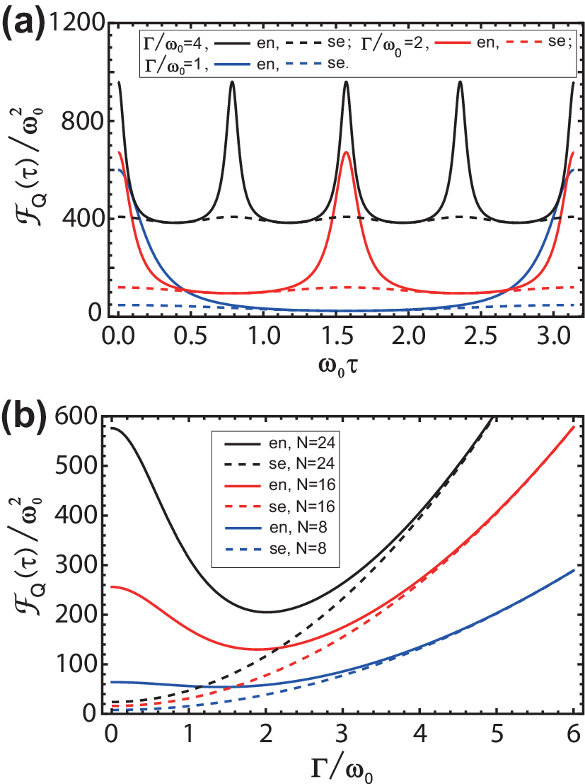
Specifically, we can obviously see from FIG. 2(a) that $\mathcal{F}^{\textrm{en}}_{Q}(\tau)\simeq\mathcal{F}^{\textrm{se}}_{Q}(\tau)$ for some time interval. In FIG. 2(b) we find that when the strength of environment $\Gamma$ is weak, $\mathcal{F}^{\textrm{en}}_{Q}(\tau)$ is larger than $\mathcal{F}^{\textrm{se}}_{Q}(\tau)$, i.e., quantum Zeno dynamics of entangled states may be harder to realize. As the increase of $\Gamma$, quantum Zeno dynamics of both cases are equally accessible. However, given “strong environment” $\Gamma/\omega_{0}\ll 1$, both $\mathcal{F}^{\textrm{en}}_{Q}(\tau)$ and $\mathcal{F}^{\textrm{se}}_{Q}(\tau)$ tend to be infinity and the ZT is confined to be so small that it makes the quantum Zeno dynamics nearly accessible as predicted in Ref. [18]. It is thus significant that the appropriate environmental interaction can be favourable for realizing QZE of entangled states compared with the case of unitary time evolution in closed system. This effect may be explained by the fact that some decoherence acts like an effective further continuous measurement on the system, therefore making the QZE more accessible. Besides, we can also figure out the optimal model of environment given the definite form of states and the definite noisy channel, which is shown in Methods. Our theory is also able to settle the case for states which are not maximally entangled but may bring new interesting results of QZE in open system.

We have investigated the accessibility of quantum Zeno dynamics in quantum open systems. The quantum Zeno dynamics in non-Markovian noise has been studied with d-FI and d-ZT when the exact master equations are used to describe the quantum open system. The more general description using operator-sum representation of the open system has also been considered and investigated. Due to the external unitary freedom of this description, an achievable upper bound of ZT is deduced via the variational methods. Although entanglement will enhance the speed of evolution and hinder QZE for unitary process[33], we have been examplified that the quantum Zeno dynamics of maximal entangled states can be realized much easier when they interacts with the proper environment than without noise. That is, the noise affecting the accuracy in the quantum parameter estimation can conversely be favorable for the accessibility of quantum Zeno dynamics of entangled states. Our work will help to stablize the system of entangled states against time evolution and noise in many quantum systems[31, 12, 7, 9].

Generally, if the survival probability for intevals, $\tau\ll 1$, can be expanded as $P(\tau)=1-F\tau^{2}/4+\mathcal{O}(\tau^{3})$, we can calculate the FI as $\mathcal{F}=[\partial_{\tau}P(\tau)]^{2}/\{P(\tau)[1-P(\tau)]\}\simeq F$. For the master equation approach, the survival probability $P(t)=\textrm{Tr}\left(\mathcal{V}(\tau)^{m}[\rho_{S}(0)]\right)={}_{S}\langle\psi_{0}|\rho_{S}(\tau)|\psi_{0}\rangle_{S}^{m}$ and we can expand the density operator $\rho_{S}(\tau)=\rho_{S}(0)+\dot{\rho}_{S}(0)\tau+\ddot{\rho}_{S}(0)\frac{\tau^{2}}{2}+\mathcal{O}(\tau^{3})$ for small time intervals. We can obtain the first order derivative as $\dot{\rho}_{S}(0)=-i[H_{S},\rho_{S}(0)]+\dot{\rho}_{S}^{I}(0)$ and for most physical cases without the Markovian approximation, $\gamma_{k}(0)=S_{k}(0)=0$ and $\dot{\rho}^{I}_{S}(0)=0$ hold for all spectral densities [22, 27, 36] with which we obtain $\langle\psi|\dot{\rho}_{S}(0)|\psi\rangle=0$. For the second order derivative, we have $\langle\psi|\ddot{\rho}_{S}(0)|\psi\rangle=-2\Delta H^{2}_{S}-\sum_{k}\dot{\gamma}_{k}(0)\textrm{Cov}_{\rho_{S}(0)}(A_{k}^{{\dagger}},A_{k})$, with which Eq. (1) can be proved.

With the optimal parametric equations, we are still able to obtain the exact form of the optimal environment that maximizes the ZT. With the optimal Hermitian operator $h_{E}^{\textrm{opt}}(\tau)=\sum_{i=1}^{N}\beta^{\textrm{opt}}(\tau)\sigma_{y,E}^{i}$, the optimal unitary time evolution is written as ${U}^{\textrm{opt}}_{SE}={u}^{\textrm{opt}}_{E}{U}_{SE}$ with ${u}^{\textrm{opt}}_{E}=\exp[{-i\int_{0}^{\tau}{h}^{\textrm{opt}}(s)ds}]$.

We would like to thank Augusto Smerzi, Wei-Bin Yan and Ying-Jie Zhang for useful discussions. This work was supported by the “973” Program (2010CB922904), NSFC (11175248) grants from the Chinese Academy of Sciences.

Y.-R. Z. and H.F. proposed the model. Y.-R.Z. calculates the results. Y.-R.Z.and H.F. analyzed the results. Y.-R.Z. and H.F. wrote the paper.

The authors declare no competing financial interests.

References

- [1] Misra, B. & Sudarshan, E. C. G. The Zeno’s paradox in quantum theory. J. Math. Phys. 18, 756 (1997).
- [2] Koshino, K. & Shimizu, A. Quantum Zeno effect by general measurements. Phys. Rep. 412, 191 (2005).
- [3] Facchi, P. & Pascazio, S. Quantum Zeno subspaces. Phys. Rev. Lett. 89, 080401 (2002).
- [4] Paz-Silva, G. A., Rezakhani, A. T., Dominy, J. M. & Lidar, D. A. Zeno effect for quantum computation and control. Phys. Rev. Lett. 108, 080501 (2012).
- [5] Maniscalco, S., Francica, F., Zaffino, R. L., Gullo, N. L. & Plastina, F. Protecting entanglement via the quantum Zeno effect. Phys. Rev. Lett. 100, 090503 (2008).
- [6] Wang, S. C., Li Y., Wang, X. B. & Kwek, L. C. Operator quantum Zeno effect: protecting quantum information with noisy two-qubit interactions. Phys. Rev. Lett. 110, 100505 (2013).
- [7] Stannigel, K., Hauke, P., Marcos, D., Hafezi, M., Diehl, S., Dalmonte, M. & Zoller, P. Constrained dynamics via the Zeno effect in quantum simulation: implementing non-Abelian lattice gauge theories with cold atoms. Phys. Rev. Lett. 112, 120406 (2014).
- [8] Zhu, B. et al. Suppressing the loss of ultracold molecules via the continuous quantum Zeno effect. Phys. Rev. Lett. 112, 070404 (2014).
- [9] Schafer, F., Herrera, I., Cherukattil, S., Lovecchio, C., Cataliotti, F. S., Caruso, F. & Smerzi, A. Experimental realization of quantum zeno dynamics. Nature Commnun. 5, 3194 (2014).
- [10] Signoles, A., Facon, A., Grosso, D., Dotsenko, I., Haroche, S., Raimond, J. M., Brune, M. & Gleyzes, S. Confined quantum Zeno dynamics of a watched atomic arrow. Nature Phys. 10, 715 (2014).
- [11] McCusker, K. T., Huang, Y. P., Kowligy, A. S. & Kumar, P. Experimental demonstration of interaction-free all-optical switching via the quantum Zeno effect. Phys. Rev. Lett. 110, 240403 (2013).
- [12] Itano, W. M., Heinzen, D. J., Bollinger, J. J. & Wineland, D. J. Quantum Zeno effect. Phys. Rev. A 41, 2295 (1990).
- [13] Bernu, J., Deléglise, S., Sayrin, C., Kuhr, S., Dotsenko, I., Brune, M., Raimond, J. M. & Haroche, S. Freezing coherent field growth in a cavity by the quantum Zeno effect. Phys. Rev. Lett. 101, 180402 (2008).
- [14] Wilkinson, S. R., Bharucha, C. F., Fischer, M. C., Madison, K. W., Morrow, P. R., Niu, Q., Sundaram, B. & Raizen, M. G. Experimental evidence for non-exponential decay in quantum tunnelling. Nature 387, 575 (1997).
- [15] Fischer, M. C., Gutierrez-Medina, B. & Raizen, M. G. Observation of the quantum Zeno and anti-Zeno effects in an unstable system. Phys. Rev. Lett. 87, 040402 (2001).
- [16] Wootters, W. K. Statistical distance and Hilbert space. Phys. Rev. D 23, 357 (1981).
- [17] Pezzé, L. & Smerzi, A. Entanglement, nonlinear dynamics, and the Heisenberg limit. Phys. Rev. Lett. 102, 100401 (2009).
- [18] Smerzi, A. Zeno dynamics, indistinguishability of state, and entanglement. Phys. Rev. Lett. 109, 150410 (2012).
- [19] Escher, B. M., de Matos Filho, R. L. & Davidovich, L. General framework for estimating the ultimate precision limit in noisy quantum-enhanced metrology. Nature Phys. 7, 406 (2011).
- [20] Escher, B. M., Davidovich, L., Zagury, N. & de Matos Filho, R. L. Quantum metrological limits via a variational approach. Phys. Rev. Lett. 109, 190404 (2012).
- [21] Nelsen, A. S. & Chuang, I. L. Quantum Computation and Quantum Information (Cambridge University Press, Cambridge, England, 2000).
- [22] Breuer, H.-P. & Petruccione, F. The Theory of Open Quantum System (Oxford University Press, New York, United States, 2003).
- [23] Alipour, S., Mehboudi, M. & Rezakhani, A. T. Quantum metrology in open systems: dissipative Cramér-Rao bound. Phys. Rev. Lett. 112, 120405 (2014).
- [24] Lu, X. M., Wang, X. G. & Sun, C. P. Quantum Fisher information flow and non-Markovian processes of open systems. Phys. Rev. A 82, 042103 (2010).
- [25] Boixo, S., Flammia, S. T., Caves, C. M. & Geremia, J. M. Generalized limits for single-parameter quantum estimation. Phys. Rev. Lett. 98, 090401 (2007).
- [26] Demkowicz-Dobrzański, R., Kołodyński, J. & Guţǎ, M. The elusive Heisenberg limit in quantumenhanced metrology. Nature Commun. 3, 1063 (2012).
- [27] Chin, A. W., Huelga, S. F. & Plenio, M. B. Quantum Metrology in Non-Markovian Environments. Phys. Rev. Lett. 109, 233601 (2012).
- [28] Huelga, S. F., Macchiavello, C., Pellizzari, T., Ekert, A. K., Plenio, M. B. & Cirac, J. I. Improvement of frequency standards with quantum entanglement. Phys. Rev. Lett. 79, 3865 (1997).
- [29] Chin, A. W., Huelga, S. F. & Plenio, M. B. Quantum metrology in non-Markovian environments. Phys. Rev. Lett. 109, 233601 (2012).
- [30] Dorner, U., Demkowicz-Dobrzański, R., Smith, B. J., Lundeen, J. S., Wasilewski, W., Banaszek, K. & Walmsley, I. A. Optimal quantum phase estimation. Phys. Rev. Lett. 102, 040403 (2009).
- [31] Kacprowicz, M., Demkowicz-Dobrzański, R., Wasilewski, W. Banaszek, K. & Walmsley, I. A. Experimental quantum-enhanced estimation of a lossy phase shift. Nature Photon. 4, 357 (2010).
- [32] Taddei, M. M., Escher, B. M., Davidovich, L. & de Matos Filho, R. L. Quantum speed limit for physical processes. Phys. Rev. Lett. 110, 050402 (2013).
- [33] del Campo, A., Egusquiza, I. L., Plenio, M. B. & Huelga, S. F. Quantum speed limits in open system dynamics. Phys. Rev. Lett. 110, 050403 (2013).
- [34] Braunstein, S. L. & Caves, C. M. Statistical distance and the geometry of quantum states. Phys. Rev. Lett. 72, 3439 (1994).
- [35] Giovannetti, V., Lloyd, S. & Maccone, L. Advances in quantum metrology. Nature Photon. 5, 222 (2011).
- [36] Facchi, P., Nakazato, H. & Pascazio, S. From the quantum Zeno to the inverse quantum Zeno effect. Phys. Rev. Lett. 86, 2699 (2001).
I Acknowledgments