CSI Feedback Reduction for MIMO Interference Alignment Thanks: The authors are with the ECE Department of the Hong Kong University of Science and Technology, Hong Kong (e-mails: {xrao,stevenr,eeknlau}@ust.hk).

Xiongbin Rao Liangzhong Ruan Student Member, IEEE and Affiliation: Vincent K.N. Lau, Fellow IEEE

Abstract

Interference alignment (IA) is a linear precoding strategy that can achieve optimal capacity scaling at high SNR in interference networks. Most of the existing IA designs require full channel state information (CSI) at the transmitters, which induces a huge CSI signaling cost. Hence it is desirable to improve the feedback efficiency for IA and in this paper, we propose a novel IA scheme with a significantly reduced CSI feedback. To quantify the CSI feedback cost, we introduce a novel metric, namely the feedback dimension. This metric serves as a first-order measurement of CSI feedback overhead. Due to the partial CSI feedback constraint, conventional IA schemes can not be applied and hence, we develop a novel IA precoder / decorrelator design and establish new IA feasibility conditions. Via dynamic feedback profile design, the proposed IA scheme can also achieve a flexible tradeoff between the degree of freedom (DoF) requirements for data streams, the antenna resources and the CSI feedback cost. We show by analysis and simulations that the proposed scheme achieves substantial reductions of CSI feedback overhead under the same DoF requirement in MIMO interference networks.

I Introduction

Due to the broadcast nature of wireless communication, interference is one of the most serious performance bottlenecks in modern wireless networks. Conventional interference management schemes either treat interference as noise or use channel orthogonalization to avoid interference. However, these schemes are far from optimal in general [1]. Interference alignment (IA), which aligns the aggregate interference from different transmitters (Txs) into a lower dimensional subspace at each receiver (Rx), achieves the optimal capacity scaling with respect to (w.r.t.) signal to noise ratio (SNR) under a broad range of network topologies [2, 3]. For instance, in a $K$ -user MIMO interference channel with $N$ antennas at each node, the IA processing achieves the throughput $\mathcal{O}(\frac{KN}{2}\cdot\log\textrm{SNR})$ [4]. This scaling law significantly dominates that achieved by conventional orthogonalization schemes ( $\mathcal{O}(N\cdot\log\textrm{SNR}$ )). As such, there has been a resurgence of research interest in IA.

Classical IA designs [5, 6, 7] assume all cross link channel state information are perfectly known at the Tx side (CSIT). In practice, it is very difficult to obtain very accurate CSIT estimation due to the limited feedback capacity and the performance of IA is highly sensitive to CSIT error [8]. This motivates the need to reduce the CSI feedback for IA in MIMO interference networks. For instance, composite Grassmannian codebooks are deployed in [9, 10] to quantize and feedback the CSI matrices for IA in MIMO interference networks. Schemes which reduce feedback overhead by adapting to the spatial/temporal correlation of CSI are proposed in [11, 12]. While the aforementioned works try to quantize and feedback entire CSI matrices, [13, 14] propose more efficient schemes by exploiting an interesting fact that IA algorithms do not need full knowledge of these matrices and hence CSI matrices can be truncated before quantization. Besides these approaches, a greedy algorithm is also proposed in [15] to reduce the size of the CSI submatrices feedback in MIMO interference networks with single stream transmission.

In this paper, we propose a novel CSI feedback scheme (with no quantization) to reduce the CSI feedback cost in MIMO interference networks under a given number of data streams (DoF) requirement. Instead of CSI truncation in [13, 14, 15], we consider a more holistic set of CSI reduction strategies by selectively feeding back the essential parts of the CSI knowledge to achieve the IA interference nulling requirements for all the data streams. We first define a novel metric, namely the feedback dimension, to quantify the cost of CSI feedback in interference networks. This metric represents the sum dimension of the Grassmannian manifolds [16, 17] that contain the CSI feedback matrices. We will illustrate in Section II that this metric serves as a first-order measurement of the CSI feedback overhead¹¹ 1 The feedback dimension measures the amount of CSI information to feedback, but it does not account for the quantization. As a result, it is proportional to the total number of bits for CSI feedback in the interference networks. Please refer to Section II for details.. We consider IA design under the proposed partial CSI feedback scheme and develop a novel precoder / decorrelator algorithm to achieve the IA interference nulling in MIMO interference networks. By introducing a dynamic feedback profile²² 2 Feedback profile refers to a parametrization of the feedback functions that determine how the CSI matrices are fed back to the Txs in the interference networks. Please refer to Section II for details. design, the proposed scheme achieves a flexible tradeoff between the performance, i.e. DoFs, and the CSI feedback cost in interference networks. To achieve these goals, there are several first order technical challenges to tackle.

•

Feedback Profile Design: To reduce the CSI feedback cost, only part of the CSI matrices can be fed back, but which part of the CSI matrices to feedback (feedback profile design) is a challenging problem. As illustrated in Example 1, a good feedback profile design can significantly reduce the feedback cost to achieve IA in interference networks. The feedback profile design in interference networks is not widely studied in the literature. In [18], the authors propose a two-hop centralized feedback profile, but the framework relies heavily on closed form precoder solutions for IA. As such, the approach in [18] can only be applied to very limited interference network topologies. In general, the feedback profile design is combinatorial and is very challenging.
•

IA Feasibility Condition: Given a number of antennas and data streams, the IA problem is well known to be not always feasible, and the feasibility condition is still not fully understood in general. The pioneering work [19] gives the feasibility condition for the single stream case by using the Bernshtein’s Theorem [20]. This work is extended to the multiple stream case in [21] by analyzing the dimension of the Algebraic Varieties [20]. In [22], a sufficient feasibility condition, which applies to general MIMO interference networks, is proposed. However, all these existing works have assumed feedback of entire CSI matrices in the interference networks. The feasibility condition of IA under partial CSI feedback in interference networks is still an open problem.
•

IA Precoder / Decorrelator Design: Conventional IA precoder algorithms [5, 6, 7] require full CSI matrices of the interference networks, and both the precoders and decorrelators are functions of the entire CSI matrices in the MIMO interference networks. However, to reduce the CSI feedback cost, only partial CSI matrices will be available at the Txs and hence, the precoders can only be a function of the partial CSI. As a result, conventional solutions for IA precoder and decorrelator designs cannot be applied in our case.

In this paper, we will address the challenges listed above by exploiting the unique features of the IA precoder / decorrelator design, and tools from Algebraic Geometry [21, 22], to reduce the CSI feedback cost without affecting the DoF performance of the network. Based on the proposed interference profile design mechanism, we derive closed form tradeoff results between the number of data streams, the antenna configuration and the CSI feedback dimension in a symmetric MIMO interference network. We also show that the proposed scheme achieves significant savings in CSI feedback cost compared with various state-of-the-art baselines.

Notations: Uppercase and lowercase boldface denote matrices and vectors respectively. The operators $(\cdot)^{T}$ , $(\cdot)^{\dagger}$ , $\textrm{rank}(\cdot)$ , $|\cdot|$ , $\textrm{tr}(\cdot)$ , $\textrm{dim}_{s}(\cdot)$ , $\textrm{dim}_{c}(\cdot)$ , $\otimes$ and $\textrm{vec}(\cdot)$ are the transpose, conjugate transpose, rank, cardinality, trace, dimension of subspace, dimension of complex manifolds [16], Kronecker product and vectorization respectively, $\mathbf{I}_{d}$ denotes $d\times d$ identity matrix, $\textrm{span}(\{\mathbf{A}_{i}\})$ denotes the vector space spanned by all the column vectors of the matrices in $\{\mathbf{A}_{i}\}$ and $d\mid M$ denotes that integer $M$ is divisible by integer $d$ .

II System Model

II-A MIMO Interference Networks

Consider a $K$ -user MIMO interference network where the $i$ -th Tx and Rx are equipped with $N_{i}$ and $M_{i}$ antennas respectively, and $d_{i}$ data streams are transmitted between the $i$ -th Tx-Rx pair. Denote the fading matrix from Tx $i$ to Rx $j$ as $\mathbf{H}_{ji}\in\mathbb{C}^{M_{j}\times N_{i}}$ .

Assumption 1 (Channel Matrices)

We assume the elements of $\mathbf{H}_{ji}$ are i.i.d. Gaussian random variables with zero mean and unit variance. The CSI $\{\mathbf{H}_{j1},\mathbf{H}_{j2},\cdots\mathbf{H}_{jK}\}$ are observable at the $j$ -th Rx and the feedback from the $j$ -th Rx will be received error-free by all the $K$ Txs.

II-B CSI Feedback Functions and Feedback Dimension

In this section, we define the partial CSI feedback as well as the notion of feedback dimension in MIMO interference networks. Since we are interested in IA, which aims at nulling off interferences between the data streams in the network, only the channel direction information³³ 3 For example, in IA designs, if $\mathbf{\mathbf{U}}^{\dagger}\mathbf{H}\mathbf{V}=\mathbf{0}$ , then we have $\mathbf{\mathbf{U}}^{\dagger}(a\mathbf{H})\mathbf{V}=0$ , $\forall a\in\mathbb{C}$ . Hence, it is sufficient to feeding back the direction information of $\mathbf{H}\in\mathbb{C}^{N\times M}$ for IA, i.e., $\{a\mathbf{H}:a\in\mathbb{C}\}$ , which is a linear space contained in $\mathbb{G}(1,MN)$ [17]. [23] is relevant, and hence, we restrict ourselves to the CSI feedback over the Grassmannian manifold. Denote $\mathbb{G}(A,B)$ as the Grassmannian manifold [17] of all $A$ -dimensional linear subspaces in $\mathbb{C}^{B\times 1}$ . Let $\mathcal{H}_{j}=(\mathbf{H}_{j1},\cdots\mathbf{H}_{jj-1},\mathbf{H}_{jj+1},\cdots\mathbf{H}_{jK})\in\prod_{\underset{\neq j}{i=1}}^{K}\mathbb{C}^{M_{j}\times N_{i}}$ be the tuple of local cross-link CSI matrices observed at the $j$ -th Rx in the MIMO interference network. To reduce CSI feedback overhead, we introduce the idea of CSI filtering, which is formulated in the following model.

Definition 1 (CSI Feedback Function)

The partial CSI feedback generated by the $j$ -th Rx is a $k_{j}$ -tuple, which can be characterized by a feedback function $F_{j}$ : $\prod_{\underset{\neq j}{i=1}}^{K}\mathbb{C}^{M_{j}\times N_{i}}\rightarrow\prod_{i=1}^{k_{j}}\mathbb{G}(A_{ji},B_{ji})$ . That is:

\mathbb{\mathcal{H}}_{j}^{fed}=F_{j}(\mathcal{H}_{j}),

(1)

where $k_{j}$ denotes the number of subspaces in $\mathbb{\mathcal{H}}_{j}^{fed}$ , $\mathbb{\mathcal{H}}_{j}^{fed}\in\mathbb{G}(A_{j1},B_{j1})\times\mathbb{G}(A_{j2},B_{j2})\times\cdots\mathbb{G}(A_{jk_{j}},B_{jk_{j}})$ is the partial CSI fed back by the $j$ -th Rx, and $\mathbb{G}(A_{jm},B_{jm})$ is the associated Grassmannian manifold with parameters $(A_{jm},B_{jm})$ containing the $m$ -th element in the CSI feedback tuple $\mathbb{\mathcal{H}}_{j}^{fed}$ . ∎

In other words, the outputs of the feedback function are a tuple of subspaces where each subspace corresponds to a point in the associated Grassmannian manifold [17]. For instance, consider two cross link CSIs $\mathbf{H}_{1},\mathbf{H}_{2}\in\mathbb{C}^{2\times 3}$ at certain Rx. If we feedback the null spaces of $\mathbf{H}_{1}$ and $\mathbf{H}_{2}$ , then this corresponds to the feedback function $F=\left(\begin{array}[]{cc}\{\mathbf{v}_{1}:\mathbf{H}_{1}\mathbf{v}_{1}=\mathbf{0}\},&\{\mathbf{v}_{2}:\mathbf{H}_{2}\mathbf{v}_{2}=\mathbf{0}\}\end{array}\right)\in\mathbb{G}(1,3)\times\mathbb{G}(1,3)$ ; If we feedback the row space of the concatenated matrix $\begin{array}[]{cc}[\mathbf{H}_{1}&\mathbf{H}_{2}]\end{array}$ , this corresponds to the feedback function $F=\textrm{span}\left([\begin{array}[]{cc}\mathbf{H}_{1}&\mathbf{H}_{2}\end{array}]^{T}\right)\in\mathbb{G}(2,6)$ . Note under given feedback functions $\{F_{j}\}$ , the partial CSI $\{F_{j}(\mathcal{H}_{j})\}$ that is fed back to the Tx side for precoder design will be known.

First, we define the feedback cost generated from the above partial CSI feedback by the feedback dimension below.

Definition 2 (Feedback Dimension)

Define the feedback dimension $D$ as the sum of the dimension of the Grassmannian manifolds [17] $\{\mathbb{G}(A_{ji},B_{ji}):i=1,\cdots k_{j},j=1,\cdots K\}$ , i.e.,

D=\sum_{j=1}^{K}\sum_{i=1}^{k_{j}}A_{ji}(B_{ji}-A_{ji}).

(2)

∎

Remark 1 (Significance of Feedback Dimension)

Note a Grassmannian manifold of dimension $D$ is locally homeomorphic [16] to $\mathbb{C}^{D\times 1}$ , and hence the feedback dimension $D$ denotes the number of complex scalars required to feedback to the Tx side. Hence, the feedback dimension serves as a first order metric of the CSI feedback overhead. For instance, given $B$ bits to feedback a CSI contained in a Grassmannian manifold with dimension $D$ , it is shown that the CSI quantization distortion scales on $\mathcal{O}\left(2^{-\frac{B}{D}}\right)$ [24, 17]. In other words, to keep a constant CSI distortion $\Delta$ , the CSI feedback bits $B$ should scale linearly with $D$ as $B=\mathcal{O}(D\log\frac{1}{\Delta})$ . Therefore, the feedback dimension is directly proportional to the total number of bits for CSI feedback.

II-C CSI Feedback Profile

In this section, we shall define the notion of feedback profile, which is a parametrization of the feedback functions $\mathcal{F}=\{F_{1},\cdots F_{K}\}$ defined in (1). We first formally define the IA problem subject to general feedback functions $\mathcal{F}$ , which is essentially a feasibility⁴⁴ 4 We are concerned with the existence of a solution in Problem 1 as well as finding it. problem [21, 22].

Problem 1 (IA Design with Partial CSI Feedback $\mathcal{F}$ )

Given the feedback functions $\mathcal{F}$ . The IA problem is to find the set of precoders $\left\{\mathbf{V}_{i}\in\mathbb{C}^{N_{i}\times d_{i}}:\forall i\right\}$ as a function of $\{F_{j}(\mathcal{H}_{j}):\forall j\}$ and decorrelator $\mathbf{U}_{j}\in\mathbb{C}^{M_{j}\times d_{j}}$ based on local CSIR (i.e., $\{\mathbf{H}_{ji}\mathbf{V}_{i}:\forall i\}$ ) $\forall j$ such that

\textrm{rank}(\mathbf{U}_{j}^{\dagger}\mathbf{H}_{jj}\mathbf{V}_{j})=d_{j},\quad\forall j,

(3)

\mathbf{U}_{j}^{\dagger}\mathbf{H}_{ji}\mathbf{V}_{i}=\mathbf{0},\;\forall i,j,\;i\neq j.

(4)

∎

Compared with conventional IA problems [19, 21, 22], Problem 1 is different and difficult because it has a new constraint on the available CSI knowledge for precoder design, i.e., $\{\mathbf{V}_{i}\}$ can only be functions of the partial CSI $\{F_{j}\}$ that is fed back. This reflects the motivation to reduce the CSI feedback cost while maintaining the IA performance in MIMO interference networks. In most conventional works of feedback designs for IA in MIMO interference network [11, 12], it has been considered that the full channel direction is fed back, (i.e., $F_{j}(\mathcal{H}_{j})=\left(\begin{array}[]{ccc}\cdots,&\{a\mathbf{H}_{ji}:a\in\mathbb{C}\},&\cdots\end{array}\right)_{i\neq j}$ ), which corresponds to a feedback dimension of $\sum_{i,j:i\neq j}(M_{j}N_{i}-1)$ in the MIMO interference networks. In the case of full channel direction feedback, the solution to Problem 1 has been widely studied [5, 6, 7], and under some sufficient conditions [19, 21, 22], Problem 1 above is feasible. However, the challenge comes when the CSI direction are not fully fed back.

Yet, for a given number of DoF requirements and antennas setups in MIMO interference networks, the full CSI direction might not always be required while IA can still be achieved. As illustrated by three motivating examples in Figure 1 (a)-(c), we show that Problem 1 can still be feasible with a much smaller feedback dimension. Denote $\mathbb{N}^{t}(\cdot)$ and $\mathbb{N}^{r}(\cdot)$ as the null space and left null space respectively, i.e., $\mathbb{N}^{t}(\mathbf{A})=\{\mathbf{u}\mid\mathbf{A}\mathbf{u}=\mathbf{0}\}$ , $\mathbb{N}^{r}(\mathbf{A})=\{\mathbf{u}\mid\mathbf{u}^{\dagger}\mathbf{A}=\mathbf{0}\}$ .

Example 1 (CSI Feedback Design I)

Consider a MIMO interference network as illustrated in Fig. 1 (a). Suppose the CSI feedback functions are given by: $F_{1}(\mathcal{H}_{1})=\mathbb{N}_{1}^{t}(\mathbf{H}_{12})$ , $F_{2}(\mathcal{H}_{2})=\mathbb{N}^{t}(\mathbf{H}_{23})$ , $F_{3}(\mathcal{H}_{3})=\mathbb{N}^{t}(\mathbf{H}_{31})$ . The precoders $\mathbf{V}_{1}$ , $\mathbf{V}_{2}$ , $\mathbf{V}_{3}$ $\in\mathbb{C}^{6\times 2}$ are designed as: $\textrm{span}(\mathbf{V}_{1})=\mathbb{N}_{1}^{t}(\mathbf{H}_{31})$ , $\textrm{span}(\mathbf{V}_{2})=\mathbb{N}^{t}(\mathbf{H}_{12})$ , $\textrm{span}(\mathbf{V}_{3})=\mathbb{N}^{t}(\mathbf{H}_{23})$ , the decorrelators $\mathbf{U}_{1}$ , $\mathbf{U}_{2}$ , $\mathbf{U}_{3}$ $\in\mathbb{C}^{4\times 2}$ are designed as: $\textrm{span}(\mathbf{U}_{1})=\mathbb{N}^{r}\left(\mathbf{H}_{13}\mathbf{V}_{3}\right)$ , $\textrm{span}(\mathbf{U}_{2})=\mathbb{N}^{r}\left(\mathbf{H}_{21}\mathbf{V}_{1}\right)$ , $\textrm{span}(\mathbf{U}_{3})=\mathbb{N}^{r}\left(\mathbf{H}_{32}\mathbf{V}_{2}\right)$ . Consequently, Problem 1 is almost surely feasible, and the feedback dimension is only 24 compared with 138 under full channel direction feedback.

Example 2 (CSI Feedback Design II)

Consider a MIMO interference network as illustrated in Fig. 1 (b). Suppose the CSI feedback functions are given by: $F_{1}(\mathcal{H}_{1})=\mathbb{N}^{t}\left((\mathbf{S}_{1}^{r})^{\dagger}\mathbf{H}_{12}\right)$ , $F_{2}(\mathcal{H}_{2})=\mathbb{N}^{t}\left((\mathbf{S}_{2}^{r})^{\dagger}\mathbf{H}_{21}\right)$ , $F_{3}(\mathcal{H}_{3})=\left(\mathbb{N}^{t}(\mathbf{H}_{32}),\mathbb{N}^{t}(\mathbf{H}_{31})\right)$ , where $\textrm{span}(\mathbf{S}_{1}^{r})=\mathbb{N}^{r}(\mathbf{H}_{13})$ and $\textrm{span}(\mathbf{S}_{2}^{r})=\mathbb{N}^{r}(\mathbf{H}_{23})$ . The precoders are designed as: $\textrm{span}(\mathbf{V}_{1})=\mathbb{N}^{t}\left((\mathbf{S}_{2}^{r})^{\dagger}\mathbf{H}_{21}\right)\bigcap\mathbb{N}^{t}(\mathbf{H}_{31})$ , $\textrm{span}(\mathbf{V}_{2})=\mathbb{N}^{t}\left((\mathbf{S}_{1}^{r})^{\dagger}\mathbf{H}_{12}\right)\bigcap\mathbb{N}^{t}(\mathbf{H}_{32})$ and $\mathbf{V}_{3}=\mathbf{I}_{2}$ . Problem 1 is also almost surely feasible, and the feedback dimension is only 32 compared with 82 under under full channel direction feedback.

Example 3 (CSI Feedback Design III)

Consider a MIMO interference network as illustrated in Fig. 1 (c). Suppose the CSI feedback functions are given by: $F_{1}(\mathcal{H}_{1})=\textrm{span}\left(\left[\begin{array}[]{cc}\mathbf{H}_{12}^{s}&\mathbf{H}_{13}^{s}\end{array}\right]^{T}\right)$ , $F_{2}(\mathcal{H}_{2})=\textrm{span}\left(\left[\begin{array}[]{cc}\mathbf{H}_{21}^{s}&\mathbf{H}_{23}^{s}\end{array}\right]^{T}\right)$ and $F_{3}(\mathcal{H}_{3})=\textrm{span}\left(\left[\begin{array}[]{cc}\mathbf{H}_{31}^{s}&\mathbf{H}_{32}^{s}\end{array}\right]^{T}\right)$ , where $\mathbf{H}_{ji}^{s}=\left[\begin{array}[]{cc}\mathbf{I}_{4}&\mathbf{0}\end{array}\right]\mathbf{H}_{ji}$ , $\forall j,i.$ Problem 1 is also almost surely feasible, and the feedback dimension is only 48 compared with 114 under full channel direction feedback.

Refer to caption — Fig. 1: Example of feedback topology design

Feedback Dimension	In Fig. 1(a)	In Fig. 1(b)	In Fig. 1(c)
Full Channel Direction Feedback	138	82	114
Proposed Feedback Schemes	24	32	48

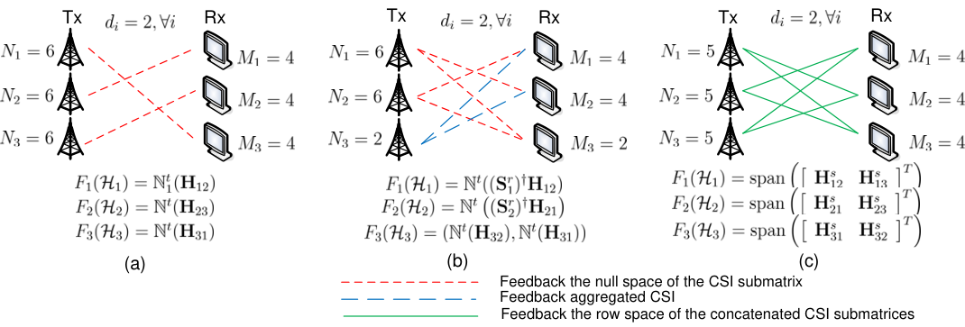
In the above three examples, Problem 1 is feasible even if the total feedback dimension are 24, 32 and 48 respectively. This represents an 83, 69 and 58 % reduction in the feedback cost compared with full channel direction feedback. The following four insights can be obtained from these three examples on how to reduce the feedback dimension at each Rx:

•

Strategy I (No Feedback for a Subset of Cross Links): In practice, IA may be achieved with no feedback for a subset of the cross links. For instance, in Example 1, cross links $\mathbf{H}_{13}$ , $\mathbf{H}_{21}$ and $\mathbf{H}_{32}$ are not fed back at all. With this strategy, Problem 1 is still feasible and the feedback dimension is significantly reduced.
•

Strategy II (Feedback of Aggregate CSI for a Subset of Cross Links): In practice, IA may be achieved by feeding back the aggregate CSI for a subset of cross links. For instance, in Example 2, link $\mathbf{H}_{13}$ is canceled by designing the decorrelator of Rx 1 in the space of $\mathbb{N}^{r}(\mathbf{H}_{13})$ . Hence, the necessary feedback information for that link is $\mathbf{S}_{1}^{r}$ ( $\textrm{span}(\mathbf{S}_{1}^{r})=\mathbb{N}^{r}(\mathbf{H}_{13})$ ), which is aggregated in the feedback CSI of the other subsets of cross links (e.g., the CSI feedback for the link from Tx 2 to Rx 1 has the form $(\mathbf{S}_{1}^{r})^{\dagger}\mathbf{H}_{12}$ ). With this strategy, Problem 1 is still feasible and the feedback dimension is reduced.
•

Strategy III (Feedback of Null Space of CSI Submatrix for a Subset of Cross Links): In practice, IA may be achieved by feeding back the null spaces for a subset of cross links. This is because the Tx can design the precoder in the channel null space to cancel that link. For instance, in Example 2, only the null spaces of $(\mathbf{S}_{1}^{r})^{\dagger}\mathbf{H}_{12}$ are fed back at Rx 1. With this strategy, Problem 1 is still feasible and the feedback dimension is reduced.
•

Strategy IV (Feedback of Row Space of CSI Submatrices for a Subset of Cross Links): In practice, IA can be achieved by feeding back the row space of the concatenated CSI submatrices for a subset of cross links. For instance, in Example 3, only $\textrm{span}\left(\left[\begin{array}[]{cc}\mathbf{H}_{12}^{s}&\mathbf{H}_{13}^{s}\end{array}\right]^{T}\right)$ is fed back at Rx 1. With this strategy, Problem 1 is still feasible and the feedback dimension is reduced.

Note that it is possible to use only one of the above strategies or apply them together and how to use these strategies depends on the DoF requirements and the antenna configurations. Furthermore, different combinations of these strategies may have significantly different IA feasibility result and final feedback cost. To begin with, we assume some structure forms for the feedback functions that can embrace all these 4 strategies. Based on the above insights, we shall first partition the cross links seen by the $j$ -th Rx into four subsets defined below.

Definition 3 (Partitioning of Cross Links)

The set of cross links seen by the $j$ -th Rx is partitioned into four subsets, namely, $\Omega_{j}^{I}$ , $\Omega_{j}^{II}$ , $\Omega_{j}^{III}$ and $\Omega_{j}^{IV}$ , according to the four strategies illustrated above. Note that $\underset{m=\{I,II,III,IV\}}{\mathbf{\bigcup}}\Omega_{j}^{m}=\{1,\cdots j-1,j+1,\cdots K\}$ , $\Omega_{j}^{m}\bigcap\Omega_{j}^{n}=\emptyset,\forall m\neq n,m,n\in\{I,II,III,IV\}$ . ∎

The feedback functions $\mathcal{F}$ are assumed to have the following structure.

Assumption 2 (Structure of Feedback Functions $\mathcal{F}$ )

The feedback functions $\mathcal{F}_{j}$ in (1) for the MIMO interference networks have the following structure:

F_{j}(\mathcal{H}_{j})=\left(\underset{\forall p\in\Omega_{j}^{III}}{\underbrace{\cdots,\mathbb{N}^{t}\left((\mathbf{S}_{j}^{r})^{\dagger}\mathbf{H}_{jp}^{s}\right),\cdots,}}\textrm{span}\left(\left[\underset{\forall q\in\Omega_{j}^{IV}}{\underbrace{\begin{array}[]{ccc}\cdots&(\mathbf{S}_{j}^{r})^{\dagger}\mathbf{H}_{jq}^{s}&\cdots\end{array}}}\right]^{T}\right)\right),

(5)

where $\mathbf{S}_{j}^{r}\in\mathbb{C}^{M_{j}^{s}\times M_{j}^{e}}$ , $(\mathbf{S}_{j}^{r})^{\dagger}\mathbf{S}_{j}^{r}=\mathbf{I}_{M_{j}^{e}}$ ,

\textrm{span}(\mathbf{S}_{j}^{r})=\mathbb{N}^{r}\left(\underset{\forall i\in\Omega_{j}^{II}}{\underbrace{\left[\begin{array}[]{ccc}\cdots&\mathbf{H}_{ji}^{s}&\cdots\end{array}\right]}}\right),

(6)

M_{j}^{e}=M_{j}^{s}-\sum_{i\in\Omega_{j}^{II}}N_{i}^{s},\forall j.

(7)

\mathbf{H}_{ji}^{s}=\left[\begin{array}[]{cc}\mathbf{I}_{M_{j}^{s}}&\mathbf{0}\end{array}\right]\mathbf{H}_{ji}\left[\begin{array}[]{c}\mathbf{I}_{N_{j}^{s}}\\ \mathbf{0}\end{array}\right],\forall j,i.

(8)

and $\{M_{i}^{s},N_{i}^{s}\}$ are parameters that characterize the feedback functions $\mathcal{F}$ . ∎

The feedback function structure is also illustrated in Fig. 2. Note that the length of the tuple $\mathbb{\mathcal{H}}_{j}^{fed}$ is $k_{j}=|\Omega_{j}^{III}|+1$ . Denote $\Omega_{j}^{III}\triangleq\{p_{1},\cdots,p_{i},\cdots\}$ , then $\mathbb{N}^{t}\left((\mathbf{S}_{j}^{r})^{\dagger}\mathbf{H}_{jp_{i}}^{s}\right)\in\mathbb{G}(A_{ji},B_{ji})$ , where $A_{ji}=M_{j}^{e}$ , $B_{ji}=N_{p_{i}}^{s}$ , $1\leq i\leq|\Omega_{j}^{III}|$ and $\textrm{span}\left(\left[\begin{array}[]{ccc}\cdots&(\mathbf{S}_{j}^{r})^{\dagger}\mathbf{H}_{jq}^{s}&\cdots\end{array}\right]_{\forall q\in\Omega_{j}^{IV}}^{T}\right)\in\mathbb{G}(A_{jk_{j}},B_{jk_{j}})$ , where $A_{jk_{j}}=\min\left(M_{j}^{e},\sum_{v\in\Omega_{j}^{IV}}N_{v}^{s}\right)$ , $B_{jk_{j}}=\sum_{v\in\Omega_{j}^{IV}}N_{v}^{s}$ , as in (1).

Note that the structural form of $\mathcal{F}$ in (5) embraces all four strategies of CSI feedback dimension reduction inspired by examples 1-3. Based on the structural form of $\mathcal{F}$ , we define the notion of feedback profile of $\mathcal{F}$ , which gives a parametrization of $\mathcal{F}$ .

Definition 4 (Feedback Profile of $\mathcal{F}$ )

Define the feedback profile of $\mathcal{F}$ as a set of parameters:

\mathcal{L}=\left\{\left\{M_{i}^{s},N_{i}^{s}:\forall i\right\},\left\{\Omega_{j}^{I},\Omega_{j}^{II},\Omega_{j}^{III},\Omega_{j}^{IV}:\forall j\right\}\right\}.

(9)

∎

Note that $\{M_{j}^{s},N_{i}^{s}\}$ controls the size of the CSI submatrices to feedback and $\left\{\Omega_{j}^{m}:m\in\{I,II,III,IV\}\}\right\}$ defines the partitioning of the cross links w.r.t. the four feedback strategies at the $j$ -th Rx. In fact, there is a 1-1 correspondence between the feedback profile $\mathcal{L}$ and the feedback function in (5). For a given feedback profile $\mathcal{L}$ (or feedback function $\mathcal{F}$ ), the total feedback dimension is given by,

D(\mathcal{L})=\sum_{j=1}^{K}M_{j}^{e}\left(\sum_{i\in\Omega_{j}^{IV}}N{}_{i}^{s}-M_{j}^{e}\right)^{+}+\sum_{j=1}^{K}\sum_{i\in\Omega_{j}^{III}}M_{j}^{e}\left(N{}_{i}^{s}-M_{j}^{e}\right).

(10)

In fact, the CSI feedback function in (6) and the associated feedback profile in (9) cover a lot of existing CSI feedback designs in the literature, and we mention a few below.

•

Special case I (Feedback Truncated CSI): In [13, 14], a truncated CSI feedback scheme is proposed in MIMO interference network. The feedback scheme corresponds to the feedback profile $\mathcal{L}$ : $M_{i}^{s}=M_{i}$ , $N_{i}^{s}=N_{i}$ , $\Omega_{j}^{I}=\Omega_{j}^{II}=\Omega_{j}^{III}=\emptyset$ , $\Omega_{j}^{IV}=\{1,\cdots,j-1,j+1,\cdots K\}$ , $\forall j$ , and feedback function $F_{j}=\textrm{span}\left(\left[\begin{array}[]{ccc}\cdots&\mathbf{H}_{ji}&\cdots\end{array}\right]_{i:\,i\neq j}^{T}\right)$ , $\forall j$ .
•

Special case II (Two-hop Centralized CSI Feedback): In [18], a centralized two-hop feedback scheme is proposed based on the closed form solutions of IA in MIMO interference network. The feedback scheme corresponds to the feedback profile $\mathcal{L}$ : $M_{i}^{s}=M_{i}$ , $N_{i}^{s}=N_{i}$ , $\Omega_{j}^{II}=\Omega_{j}^{III}=\emptyset$ , $\Omega_{j}^{IV}=\{a_{j},b_{j}\}$ , $\Omega_{j}^{I}=\{1,\cdots,j-1,j+1,\cdots K\}/\Omega_{j}^{IV}$ , $\forall j$ , where $(a_{1},b_{1})=(2,3),$ $(a_{2},b_{2})=(3,4),$ … $(a_{K-1},b_{K-1})=(K,1)$ , $(a_{K},b_{K})=(1,2)$ , and the feedback function $F_{j}=\textrm{span}\left(\left[\begin{array}[]{cc}\mathbf{H}_{ja_{j}}&\mathbf{H}_{jb_{j}}\end{array}\right]^{T}\right)=\textrm{span}\left(\left[\mathbf{H}_{jb_{j}}^{-1}\begin{array}[]{cc}\mathbf{H}_{ja_{j}}&\mathbf{I}\end{array}\right]^{T}\right)$ , $\forall j$ .

III Design of IA Precoders and Decoders under a Feedback Profile

In this section, we focus on solving the IA precoders and decorrelators design in Problem 1 for a given feedback profile $\mathcal{L}$ . Specifically, we first impose some structural properties on the precoders / decorrelators so as to satisfy the constraints of partial CSI feedback. Based on the proposed structures, we transform Problem 1 into an equivalent bi-convex problem and derive an iterative solution.

III-A Structure of IA Precoders / Decorrelators

One unique challenge of the IA precoders / decorrelators design in Problem 1 is that the precoders can only be adaptive to the partial CSI knowledge at the Txs. This is fundamentally different from conventional IA precoders / decorrelators design in which both can be adaptive to the entire CSI matrices. To address this challenge, we shall first impose some structures in the precoders / decorrelators so as to utilize the partial CSI obtained from combinations of feedback strategies⁵⁵ 5 Notice that Strategy I does not feedback the CSI for the chosen subset of cross links. I-IV.

•

Utilization of Partial CSI from Feedback Strategy II: From feedback strategy II, we can obtain the aggregated CSI with $\mathbf{S}_{j}^{r}$ , which spans $\mathbb{N}^{r}\left(\left[\begin{array}[]{ccc}\cdots&\mathbf{H}_{ji}^{s}&\cdots\end{array}\right]_{\forall i\in\Omega_{j}^{II}}\right)$ . Hence, we can design the decorrelator of Rx $j$ in the space of $\textrm{span}(\mathbf{S}_{j}^{r})$ , and consequently, all interference from Tx $i$ to Rx $j$ , where $i\in\Omega_{j}^{II}$ , is eliminated (note $(\mathbf{S}_{j}^{r})^{\dagger}\mathbf{H}_{ji}^{s}=\mathbf{0}$ , $\forall j,i\in\Omega_{j}^{II}$ ).

•

Utilization of Partial CSI from Feedback Strategy III: From feedback strategy III, we obtain the following set of spaces $\left\{\mathbb{N}^{t}\left((\mathbf{S}_{j}^{r})^{\dagger}\mathbf{H}_{ji}^{s}\right):\forall j,i\in\Omega_{j}^{III}\right\}$ . Based on this information, we obtain the set of matrices $\{\mathbf{S}_{i}^{t}\in\mathbb{C}^{N_{i}^{s}\times N_{i}^{e}}:\forall i\}$ , where $(\mathbf{S}_{i}^{t})^{\dagger}\mathbf{S}_{i}^{t}=\mathbf{I}_{N_{i}^{e}}$ ,

\textrm{ span }\left(\mathbf{S}_{i}^{t}\right)=\underset{\forall j:\,i\in\Omega_{j}^{III}}{\bigcap}\mathbb{N}^{t}\left((\mathbf{S}_{j}^{r})^{\dagger}\mathbf{H}_{ji}^{s}\right)

(11)

and

N_{i}^{e}=N_{i}^{s}-\sum_{j:\,i\in\Omega_{j}^{III}}M_{j}^{e},\forall i.

(12)

Hence, we can design the precoder of Tx $i$ in the space of $\textrm{span}(\mathbf{S}_{i}^{t})$ , and consequently, all the interference from Tx $i$ to Rx $j$ , where $i\in\Omega_{j}^{III}$ , is eliminated (note $(\mathbf{S}_{j}^{r})^{\dagger}\mathbf{H}_{ji}^{s}\mathbf{S}_{i}^{t}=\mathbf{0}$ , $\forall j,i\in\Omega_{j}^{III}$ ).

•

Utilization of Partial CSI from Feedback Strategy IV: From feedback strategy IV, we obtain the following set of spaces, i.e., $\left\{\textrm{span}\left(\left[\begin{array}[]{ccc}\cdots&(\mathbf{S}_{j}^{r})^{\dagger}\mathbf{H}_{ji}^{s}&\cdots\end{array}\right]_{i\in\Omega_{j}^{IV}}^{T}\right):\forall j\right\}$ . Based on this information, we find the set of matrices $\{\mathbf{\tilde{H}}_{j}:\forall j\}$ , where $\textrm{span}(\mathbf{\tilde{H}}_{j}^{T})=\textrm{span}\left(\left[\begin{array}[]{ccc}\cdots&(\mathbf{S}_{j}^{r})^{\dagger}\mathbf{H}_{ji}^{s}&\cdots\end{array}\right]_{i\in\Omega_{j}^{IV}}^{T}\right)$ , and there must exist an invertible matrix $\mathbf{R}_{j}\in\mathbb{C}^{M_{j}^{e}\times M_{j}^{e}}$ such that

\mathbf{\tilde{H}}_{j}=\mathbf{R}_{j}\left[\begin{array}[]{ccc}\cdots&(\mathbf{S}_{j}^{r})^{\dagger}\mathbf{H}_{ji}^{s}&\cdots\end{array}\right]_{i\in\Omega_{j}^{IV}}.

(13)

Hence, we can obtain $\left\{\mathbf{R}_{j}(\mathbf{S}_{j}^{r})^{\dagger}\mathbf{H}_{ji}^{s}:\forall j,i\in\Omega_{j}^{IV}\right\}$ , and the precoders / decorrelators can be designed based on these effective CSI matrices such that the interference from Tx $p$ to Rx $q$ , $\forall(p,q)\in\{(j,i):\forall j,i\in\Omega_{j}^{IV}\}$ can be aligned into a lower dimensional subspace at the Rxs.

Based on these insights, we propose the following structures for $\{\mathbf{V}_{i},\mathbf{U}_{j}\}$ in the MIMO interference networks.

Definition 5 (IA Precoders / Decorrelators Structure)

The IA solutions $\{\mathbf{V}_{i},\mathbf{U}_{j}\}$ for Problem 1 have the following structure:

\mathbf{V}_{i}=\left[\begin{array}[]{c}\mathbf{S}_{i}^{t}\mathbf{V}_{i}^{a}\\ \mathbf{0}\end{array}\right],\quad\mathbf{U}_{j}=\left[\begin{array}[]{c}\mathbf{S}_{j}^{r}(\mathbf{R}_{j})^{\dagger}\mathbf{U}_{j}^{a}\\ \mathbf{0}\end{array}\right],

(14)

where $\mathbf{V}_{i}^{a}\in\mathbb{C}^{N_{i}^{e}\times d_{i}}$ , $\mathbf{U}_{j}^{a}\in\mathbb{C}^{M_{j}^{e}\times d_{j}}$ , $M_{j}^{e}$ and $N_{i}^{e}$ are given in (7) and (12) respectively. ∎

Note the above solution structures (14) automatically satisfy the IA constraints (4) for links from Tx $i$ to Rx $j$ , where $i\in\Omega_{j}^{II}\Omega_{j}^{III}$ , $\forall j$ and they satisfy the partial CSI feedback constraints in Problem 1. However, the constraints that $\{\mathbf{H}_{ji}:\forall j,i\in i\in\Omega_{j}^{I}\}$ are not fed back and hence can not be utilized to design the precoders, still make it hard to apply classical Algebraic Geometry theory [21, 22] to the study of Problem 1. To cope with this, we further transform Problem 1 to the following feasibility problem in which all the hidden constraints on the available CSI knowledge are explicitly handled.

Problem 2 (Transformed IA Problem)

Find $\mathbf{V}_{i}^{a}\in\mathbb{C}^{N_{i}^{e}\times d_{i}}$ , $\forall i$ and $\mathbf{U}_{j}^{b}\in\mathbb{C}^{M_{j}^{e}\times d_{j}^{0}}$ , $\forall j$ such that $\{\mathbf{V}_{i}^{a},\mathbf{U}_{j}^{b}\}$ satisfy

\textrm{rank}(\mathbf{V}_{i}^{a})=d_{i},\;\forall i,\,\textrm{rank}(\mathbf{U}_{j}^{b})=d_{j}^{0},\;\forall j,

(15)

(\mathbf{U}_{j}^{b})^{\dagger}\mathbf{G}_{ji}\mathbf{V}_{i}^{a}=\mathbf{0},\,\forall j,i\in\Omega^{IV},

(16)

where $\mathbf{G}_{ji}=\mathbf{R}_{j}(\mathbf{S}_{j}^{r})^{\dagger}\mathbf{H}_{ji}^{s}\mathbf{S}_{i}^{t}$ , $d_{j}^{0}=d_{j}+\sum_{i\in\Omega_{j}^{I}}d_{i}$ , $\forall j,i\in\Omega^{IV}$ . ∎

Lemma 1 (Equivalence of Problem 1 and Problem 2)

For a given feedback profile $\mathcal{L}$ , under the precoders / decorrelators structures in (14), we have almost surely that Problem 1 is feasible iff Problem 2 is feasible. Furthermore, if $\{\mathbf{V}_{i}^{a},\mathbf{U}_{j}^{b}\}$ are the solution of Problem 2, then

\mathbf{V}_{i}=\left[\begin{array}[]{c}\mathbf{S}_{i}^{t}\mathbf{V}_{i}^{a}\\ \mathbf{0}\end{array}\right],\mathbf{U}_{j}=v_{d_{j}}\left(\sum_{i\neq j}\left(\mathbf{H}_{ji}\mathbf{V}_{i}\right)\left(\mathbf{H}_{ji}\mathbf{V}_{i}\right)^{\dagger}\right),\forall i,j

(17)

are solution of Problem 1, where $v_{(d)}(\mathbf{A})$ is the matrix of eigenvectors corresponding to the $d$ least eigenvalues of a Hermitian matrix $\mathbf{A}$ .

Proof:

Please See Appendix -A. ∎

Note that Lemma 1 simplifies the original Problem 1 by eliminating the IA constraints on all links from Tx $i$ to Rx $j$ , where $i\in\Omega_{j}^{I}\cup\Omega_{j}^{II}\Omega_{j}^{III}$ , $\forall j$ . Furthermore, the solutions obtained will automatically satisfy the partial CSI knowledge constraints.

III-B IA Precoders / Decorrelators Design

In this section, we will derive solutions for Problem 1 by solving Problem 2. Note that Problem 2 is a bi-convex problem w.r.t. $\{\mathbf{V}_{i}^{a}\}$ and $\{\mathbf{U}_{j}^{b}\}$ . As a result, we shall apply alternating optimization techniques [5, 7] to obtain a local optimal solution. The algorithm details are outlined below:

\min_{\{\mathbf{U}_{j}^{b}\in\mathbb{C}^{M_{j}^{e}\times d_{j}^{0}}:(\mathbf{U}_{j}^{b})^{\dagger}\mathbf{U}_{j}^{b}=\mathbf{I}_{d_{j}^{0}},\forall j\}}I=\underset{j,i:\,i\in\Omega_{j}^{IV}}{\sum}\textrm{tr}\left(\left(\mathbf{U}_{j}^{b}\mathbf{G}_{ji}\mathbf{V}_{i}^{a}\right)\left(\mathbf{U}_{j}^{b}\mathbf{G}_{ji}\mathbf{V}_{i}^{a}\right)^{\dagger}\right).

(18)

\min_{\{\mathbf{V}_{i}^{a}\in\mathbb{C}^{N_{i}^{e}\times d_{i}}:(\mathbf{V}_{j}^{a})^{\dagger}\mathbf{V}_{j}^{a}=\mathbf{I}_{d_{j}},\forall i\}}I=\underset{j,i:\,i\in\Omega_{j}^{IV}}{\sum}\textrm{tr}\left(\left(\mathbf{U}_{j}^{b}\mathbf{G}_{ji}\mathbf{V}_{i}^{a}\right)\left(\mathbf{U}_{j}^{b}\mathbf{G}_{ji}\mathbf{V}_{i}^{a}\right)^{\dagger}\right).

(19)

Algorithm 1 (Iterative Precoder / Decorrelator Design):

•

Step 1 (Initialization): Randomly initialize $\mathbf{V}_{i}^{a}\in\mathbb{C}^{N_{i}^{e}\times d_{i}}$ , $\mathbf{U}_{i}^{b}\in\mathbb{\mathbb{C}}^{M_{i}^{e}\times d_{i}^{0}}$ , $\forall i$ . Initialize $\mathbf{G}_{ji}=\mathbf{R}_{j}(\mathbf{S}_{j}^{r})^{\dagger}\mathbf{H}_{ji}^{s}\mathbf{S}_{i}^{t}$ , $\forall j,i\in\Omega_{j}^{IV}$ , where $\mathbf{S}_{i}^{t}$ is given in (11).
•

Step 2 (Update $\{\mathbf{U}_{j}^{b}\}$ by Solving (18)): Update $\mathbf{U}_{j}^{b}=v_{d_{j}^{0}}(\mathbf{E}_{j})$ where $\mathbf{E}_{j}=\underset{i:i\in\Omega_{j}^{IV}}{\sum}\left(\mathbf{G}_{ji}\mathbf{V}_{i}^{a}\right)\left(\mathbf{G}_{ji}\mathbf{V}_{i}^{a}\right)^{\dagger}$ , $\forall j$ .
•

Step 3 (Update $\{\mathbf{V}_{i}^{a}\}$ by Solving (19)): Update $\mathbf{V}_{i}^{a}=v_{d_{i}}(\mathbf{T}_{i})$ , where $\mathbf{T}_{i}=\underset{j:\,i\in\Omega_{j}^{IV}}{\sum}\left(\mathbf{G}_{ji}^{\dagger}\mathbf{U}_{j}^{b}\right)\left(\mathbf{G}_{ji}^{\dagger}\mathbf{U}_{j}^{b}\right)^{\dagger}$ , $\forall i$ .
•

Repeat Step 2 and Step 3 until convergence. From the converged solution of $\{\mathbf{V}_{i}^{a},\mathbf{U}_{j}^{b}\}$ above, we can get the overall solution $\{\mathbf{V}_{i},\mathbf{U}_{j}\}$ of Problem 1 using (17). ∎

Remark 2 (Characterization of Algorithm 1)

Note Algorithm 1 can automatically adapt to the partial CSI feedback constraint in Problem 1 for a given $\mathcal{L}$ . On the other hand, Algorithm 1 converges almost surely because the total interference leakage $I$ in (18) and (19) is non-negative and it is monotonically decreasing in the alternating updates of Step 2 and Step 3. Note that if the total interference leakage $I$ at the converged local optimal point is 0, then the solution is a feasible solution of Problem 1.

IV Feasibility Conditions and Feedback Profile Design

In this section, we study the feasibility conditions of Problem 1 under a feedback profile $\mathcal{\mathcal{L}}$ and the precoder / decorrelator structure in (14). Based on the feasibility conditions, a low complexity greedy algorithm is further proposed to derive a feedback profile $\mathcal{L}$ for a given DoF requirements in the interference network. The derived feedback profile can achieve substantial savings in the total CSI feedback dimension required to achieve the given DoFs.

IV-A Feasibility Conditions under Feedback Profile $\mathcal{L}$

In this section, we extend the results in Algebraic Geometry [21, 22] and establish new feasibility conditions for IA under reduced CSI feedback dimension. We first have the following property regarding Problem 2.

Lemma 2 (Transformation Invariant Property)

The invertible matrices $\{\mathbf{R}_{j}\}$ do not affect the feasibility conditions of Problem 2, i.e., Problem 2 is feasible when $\mathbf{R}_{j}=\mathbf{I}$ , $\forall j$ iff it is feasible under any invertible matrix $\mathbf{R}_{j}$ , $\forall j$ .

Proof:

Please see Appendix -B for details.∎

Remark 3 (Role of Lemma 2)

From Lemma 2, we further conclude that it is sufficient to feedback the row space of the concatenated CSI matrices, i.e., $\textrm{span}\left(\left[\begin{array}[]{ccc}\cdots&(\mathbf{S}_{j}^{r})^{\dagger}\mathbf{H}_{ji}^{s}&\cdots\end{array}\right]_{i\in\Omega_{j}^{IV}}^{T}\right)$ at each Rx in order to satisfy the IA constraints in (15)-(16). This is illustrated in the IV-th feedback strategy in our proposed feedback structure in (6). In general, the feedback dimension will be reduced by adopting feedback strategy IV, while the feasibility of Problem 2 is not affected (i.e., the same as feeding back $\left[\begin{array}[]{ccc}\cdots&(\mathbf{S}_{j}^{r})^{\dagger}\mathbf{H}_{ji}^{s}&\cdots\end{array}\right]_{i\in\Omega_{j}^{IV}}$ ).

Since $\{\mathbf{R}_{j}\}$ do not affect the problem feasibility, we investigate the feasibility conditions under $\mathbf{R}_{j}=\mathbf{I}$ , $\forall j$ without loss of generality. The necessary feasibility conditions are established as follows.

Theorem 1 (Necessary Feasibility Conditions)

Given a feedback profile $\mathcal{L}$ and the precoder / decorrelator structure in (14), if Problem 1 is feasible, then the following three conditions must be satisfied: 1) $N_{i}^{e}\geq d_{i}$ , $\forall i$ ; 2) $M_{j}^{e}\geq d_{j}^{0}$ , $\forall j$ ; 3) Denote $V_{i}=d_{i}(N_{i}^{e}-d_{i})$ , $\forall i$ , $U_{j}=d_{j}^{0}(M_{j}^{e}-d_{j}^{0})$ , $\forall j$ ; $C_{ji}=d_{j}^{0}d_{i}$ , and $V_{i}$ , $U_{j}$ and $C_{ji}$ satisfy

\sum_{j:\,(j,i)\in\Omega_{sub}}U_{i}+\sum_{i:\,(j,i)\in\Omega_{sub}}V_{i}\geq\sum_{j,i:\,(j,i)\in\Omega_{sub}}C_{ji},\quad\forall\Omega_{sub}\subseteq\{(j,i):\,\forall j,i\in\Omega_{j}^{IV}\}.

(20)

Proof:

Please see Appendix -C for details. ∎

Next, we try to study the sufficient feasibility conditions for Problem 1. To ensure that $\textrm{rank}(\mathbf{V}_{i}^{a})=d_{i}$ and $\textrm{rank}(\mathbf{U}_{j}^{b})=d_{j}^{0}$ in Problem 2, it is sufficient to assume that the first $d_{i}\times d_{i}$ , $d_{j}^{0}\times d_{j}^{0}$ submatrix of $\mathbf{V}_{i}^{a}$ , $\mathbf{U}_{j}^{b}$ , denoted by $\mathbf{V}_{i}^{(1)}$ , $\mathbf{U}_{j}^{(1)}$ , are invertible $\forall i,\>j$ . Under this assumption, we further denote $\mathbf{\tilde{V}}_{i}\in\mathbb{C}^{(N_{i}^{e}-d_{i})\times d_{i}}$ , $\mathbf{\tilde{U}}_{j}\in\mathbb{C}^{(M_{j}^{e}-d_{j}^{0})\times d_{j}^{0}}$ , and the four submatrices of $\mathbf{G}_{ji}$ in (16), i.e., $\mathbf{G}_{ji}^{(1)}\in\mathbb{C}^{d_{j}^{0}\times d_{i}}$ , $\mathbf{G}_{ji}^{(2)}\in\mathbb{C}^{(M_{j}^{e}-d_{j}^{0})\times d_{i}}$ , $\mathbf{G}_{ji}^{(3)}\in\mathbb{C}^{d_{j}^{0}\times(N_{i}^{e}-d_{i})}$ , $\mathbf{G}_{ji}^{(4)}\in\mathbb{C}^{(M_{j}^{e}-d_{j}^{0})\times(N_{i}^{e}-d_{i})}$ , as follows:

\left[\begin{array}[]{c}\mathbf{I}_{d_{i}}\\ \mathbf{\tilde{V}}_{i}\end{array}\right]=\mathbf{V}_{i}^{a}\left(\mathbf{V}_{i}^{(1)}\right)^{-1},\left[\begin{array}[]{c}\mathbf{I}_{d_{j}^{0}}\\ \mathbf{\tilde{U}}_{j}\end{array}\right]=\mathbf{U}_{j}^{b}\left(\mathbf{U}_{j}^{(1)}\right)^{-1},\mathbf{G}_{ji}=\left[\begin{array}[]{cc}\mathbf{G}_{ji}^{(1)}&\mathbf{G}_{ji}^{(3)}\\ \mathbf{G}_{ji}^{(2)}&\mathbf{G}_{ji}^{(4)}\end{array}\right].

Hence, equation (16) becomes

\mathbf{G}_{ji}^{(1)}+\mathbf{\tilde{U}}_{j}^{\dagger}\mathbf{G}_{ji}^{(2)}+\mathbf{G}_{ji}^{(3)}\mathbf{\tilde{V}}_{i}+\mathbf{\tilde{U}}_{j}^{\dagger}\mathbf{G}_{ji}^{(4)}\mathbf{\tilde{V}}_{i}=\mathbf{0},\;\forall j,i\in\Omega_{j}^{IV}.

(21)

Based on the equation sets in (21), the sufficient feasibility conditions are established as follows.

Theorem 2 (Sufficient Feasibility Conditions)

Given a feedback profile $\mathcal{L}$ and the precoder / decorrelator structure structure in (14), if $N_{i}^{e}\geq d_{i}$ , $M_{i}^{e}\geq d_{i}^{0}$ $\forall i$ , and the row vectors of all the matrices $\{\mathbf{X}_{ji}:\forall j,i\in\Omega_{j}^{IV}\}$ are linearly independent, then Problem 1 is feasible almost surely, where

\begin{array}[]{ccccccc}\underset{d_{i}d_{j}^{0}\times\overline{M}}{\underbrace{\mathbf{X}_{ji}}}&=&\underset{d_{i}d_{j}^{0}\times m_{ji}}{[\underbrace{\mathbf{0}}}&(\mathbf{G}_{ji}^{(2)})^{T}\otimes\mathbf{I}_{d_{j}^{0}}&\underset{d_{i}d_{j}^{0}\times n_{ji}}{\underbrace{\mathbf{0}}}&\mathbf{I}_{d_{i}}\otimes\mathbf{G}_{ji}^{(3)}&\underset{d_{i}d_{j}^{0}\times k_{ji}}{\underbrace{\mathbf{0}}]}\end{array}

(22)

and $\overline{M}=\sum_{i=1}^{K}\left(d_{i}^{0}(M_{i}^{e}-d_{i}^{0})+d_{i}(N_{i}^{e}-d_{i})\right)$ , $m_{ji}=\sum_{p=1}^{j-1}d_{p}^{0}(M_{p}^{e}-d_{p}^{0})$ , $n_{ji}=\sum_{p=j+1}^{K}d_{p}^{0}(M_{p}^{e}-d_{p}^{0})+\sum_{q=1}^{i-1}d_{q}(N_{q}^{e}-d_{q})$ , $k_{ji}=\sum_{q=i+1}^{K}d_{q}(N_{q}^{e}-d_{q})$ .

Moreover, under a given feedback profile $\mathcal{L}$ , if the matrices $\{\mathbf{X}_{ji}\}$ under a random channel realization $\{\mathbf{H}_{ji}:\forall j,i\}$ have linearly independent row vectors, Problem 1 is feasible for all channel realizations almost surely.

Proof:

Please See Appendix -D. ∎

Corollary 1 (Feasibility Conditions in Divisible Cases)

When $d_{i}=d$ , $\forall i$ , and all $M_{i}^{s}$ , $N_{i}^{s}$ are divisible by the data stream, i.e., $d\mid M_{i}^{s}$ , $d\mid N_{i}^{s}$ , $\forall\,i$ , the three conditions in Theorem 1 are also sufficient.

Proof:

Please see Appendix -E. ∎

Remark 4 (Backward Compatibility with Previous Results)

If the row space of the concatenated channel matrices of all cross links are fed back, i.e., $M_{i}^{s}=M_{i}$ , $N_{i}^{s}=N_{i}$ , $\forall i$ , $\Omega_{j}^{I}=\Omega_{j}^{II}=\Omega_{j}^{III}=\emptyset$ , $\Omega_{j}^{IV}=\{1,\cdots j-1,j+1,\cdots K\}$ $\forall j$ , then $M_{i}^{e}=M_{i}$ , $d_{j}^{0}=0$ , $N_{j}^{e}=N_{j}$ , $\forall i,\,j$ , and Corollary 1 reduces to the results (Theorem 2) in [21].

IV-B CSI Feedback Profile Design $\mathcal{L}$

In this section, we focus on the design of the feedback profile to reduce the total CSI feedback cost (feedback dimension) required to achieve a given DoF requirement of the $K$ data streams $\{d_{1},d_{2},\cdots d_{K}\}$ in the MIMO interference networks. Specifically, we would like to find a feedback profile $\mathcal{L}$ that satisfies the following constraints:

Problem 3 (Feedback Profile Design $\mathcal{L}$ )

	$\displaystyle\bigcup_{m\in\{I,II,III,IV\}}\Omega_{j}^{m}=\{1,\cdots K\}/\{j\},\,\forall j,$		(23)
	$\displaystyle\Omega_{j}^{m}\bigcap\Omega_{j}^{n}=\emptyset,\forall m\neq n,\,\forall j,$		(24)
	$\displaystyle N_{i}^{e}\geq d_{i},\,M_{i}^{e}\geq d_{i}^{0},\,\forall i,$		(25)
	$\displaystyle\{\mathbf{X}_{ji}\}\textrm{ have linearly independent row vectors,}\,\forall j,i\in\Omega_{j}^{IV}$		(26)

where $\{\mathbf{X}_{ji}\}$ are given in Theorem 2 and $N_{i}^{e}$ , $M_{i}^{e}$ and $d_{i}^{0}$ are given in (7), (12) and (15) respectively. ∎

Note that constraints (23), (24) come from the feedback profile structure in Assumption 2, constraints (25) and (26) come from the the feasibility conditions of Problem 1 (Theorem 2).

A feedback profile that satisfies the above constraints is called a feasible feedback profile. Ideally, we would like to find a feasible feedback profile $\mathcal{L}$ that induces a small feedback dimension. However, the design of feedback profile $\mathcal{L}$ is highly non-trivial due to the combinatorial nature, and doing exhaustive search has exponential complexity in $\mathcal{O}\left((N)^{2K}4^{K(K-1)}(KN)^{3}\right)$ (see equation (31)). In the following, we propose a low complexity greedy algorithm to derive a feasible feedback profile $\mathcal{L}$ . We show in Section V and VI that the associated feedback cost is quite small compared with conventional state-of-the-art baselines.

The details of the greedy algorithm are summarized as follows:

Algorithm 2 (Greedy Feedback Profile Design $\mathcal{L}$ ):

•

Step 1 (Initialization and Antenna Pruning): Initialize $t=1$ , $\Omega_{j}^{I}=\Omega_{j}^{II}=\Omega_{j}^{III}=\emptyset$ , $\Omega_{j}^{IV}=\{1,\cdots j-1,j+1,\cdots K\}$ , $\forall j$ , $M_{i}^{s}=\min(M_{i},\sum_{i}d_{i})$ , $N_{i}^{s}=\min(N_{i},\sum_{i}d_{i})$ , $\forall i$ in $\mathcal{L}(t)$ .

•

Step 2 (Priority Computation): Compute the priority $p(s)$ of update strategy $s$ on current $\mathcal{L}(t)$ as

p(s)=\left(I_{\underset{\Delta V(s)\leq 0\}}{\{\Delta D(s)\geq 0}}\Delta D(s)\left(-\Delta V(s)+1\right)\alpha+I_{\underset{\Delta V(s)>0\}}{\{\Delta D(s)\geq 0}}\frac{\Delta D(s)}{\Delta V(s)}\right),\forall s\in\mathcal{P}\left(\mathcal{L}(t)\right)

(27)

where $\mathcal{P}\left(\mathcal{L}(t)\right)$ is the space of the update strategies on current $\mathcal{L}(t)$ and is given by

\mathcal{P}(\mathcal{L}(t))=\left\{\left\{S^{I}(j,i),S^{II}(j,i),S^{III}(j,i):\forall j,i\in\Omega_{j}^{IV}\right\},\{S^{IV}(i),S^{V}(i),S^{VI}(i):\forall i\}\right\},

(28)

$S^{I}(\cdot)\cdots S^{VI}(\cdot)$ are different types of update operations described in Table I (note that all these update strategies could potentially reduce the feedback dimension); $I_{\{\cdot\}}$ denotes the indicator function and $\Delta D(s)$ denotes the dimension reduction via $s$ , i.e.,

\Delta D(s)=D\left(\mathcal{L}(t+1\mid s)\right)-D\left(\mathcal{L}(t)\right),

(29)

where $D(\mathcal{L})$ is in (10) and $\mathcal{L}(t+1\mid s)$ is the feedback profile obtained by updating $\mathcal{L}(t)$ with $s$ ; $\Delta V(s)$ is the consumed free variables with strategy $s$ , i.e.,

\Delta V(s)=V\left(\mathcal{L}(t+1\mid s)\right)-V\left(\mathcal{L}(t)\right),

(30)

where $V(\mathcal{L})=\sum_{j}U_{j}+\sum_{i}V_{i}-\sum_{j,i:\,\Omega_{j}^{IV}=1}C_{ji}$ , and $U_{j}$ , $V_{i}$ , $C_{ji}$ are in Theorem 1; $\alpha$ is chosen to be $\alpha=K(\sum d_{i})^{2}$ .

•

Step 3 (Priority Sorting): Sort $\left\{p(s):\forall s\in\mathcal{P}\left(\mathcal{L}(t)\right)\right\}$ in descending order, i.e., $\mathcal{P}\left(\mathcal{L}(t)\right)\triangleq\{s_{1},\cdots s_{J}\}$ , $J=|\mathcal{P}\left(\mathcal{L}(t)\right)|$ and $p(s_{1})\geq p(s_{2})\geq\cdots\geq p(s_{J})$ . Initialize the index $k=1$ .
•

Step 4 (Greedy Update on $\mathcal{L}$ ):
- –
  
  A (Update Trial and Stopping Condition): If $k\leq|\mathcal{P}\left(\mathcal{L}(t)\right)|$ and $p(s_{k})\geq 0$ , then choose $s=s_{k}$ and update $\mathcal{L}$ as: $\mathcal{L}(t)\overset{s}{\rightarrow}\mathcal{L}(t+1\mid s)$ ; Else, exit the algorithm.
- –
  
  B (Feasibility Checking): If $\mathcal{L}(t+1\mid s)$ is feasible by Theorem 2, then set $t=t+1$ , $\mathcal{L}(t+1)=\mathcal{L}(t+1\mid s)$ and go to Step 2; Else, set $k=k+1$ and go to Step 4 A. ∎

update strategy	update $\mathcal{L}(t)$ as
$S^{I}(j,i)$	$\Omega_{j}^{I}=\Omega_{j}^{I}\bigcup\{i\},\Omega_{j}^{IV}=\Omega_{j}^{IV}/\{i\}$
$S^{II}(j,i)$	$\Omega_{j}^{II}=\Omega_{j}^{II}\bigcup\{i\},\Omega_{j}^{IV}=\Omega_{j}^{IV}/\{i\}$
$S^{III}(j,i)$	$\Omega_{j}^{III}=\Omega_{j}^{III}\bigcup\{i\},\Omega_{j}^{IV}=\Omega_{j}^{IV}/\{i\}$
$S^{IV}(i)$	$N_{i}^{s}=d_{i},\Omega_{j}^{IV}=\emptyset,\Omega_{j}^{II}=\Omega_{j}^{II}\bigcup\Omega_{j}^{IV}$
$S^{V}(i)$	$M_{i}^{s}=M_{i}^{s}-1$
$S^{VI}(i)$	$N_{i}^{s}=N_{i}^{s}-1$

TABLE I: Description of different update strategies on

\mathcal{L}

Remark 5 (Design Motivation of Algorithm 2)

Given current feedback profile $\mathcal{L}(t)$ , different strategies in $\mathcal{P}(\mathcal{L}(t))$ in (28) have different features. For instance, they reduce the feedback dimension differently (i.e., $\Delta D(s)$ ) and consume different numbers of free variables (i.e., $\Delta V(s)$ ). Intuitively, a strategy with a larger ratio of dimension reduction versus variables consumption (i.e., $\frac{\Delta D(s)}{\Delta V(s)}$ ) should have higher priority, as in this way, we may achieve more aggregate feedback dimension reduction. On the other hand, strategies with $\Delta D(s)>0$ , $\Delta V(s)\leq 0$ are given relatively higher priority, as illustrated in (27) (due to the factor $\alpha$ in (27)), because these strategies reduce the feedback dimension (i.e., $\Delta D(s)>0$ ) while they do not consume the free variables (i.e., $\Delta V(s)\leq 0$ ).

Remark 6 (Complexity of Greedy Feedback Profile Design)

We compare the complexity of exhaustive search and the proposed design algorithm as follows. For simplicity, assume that $M_{i}=N_{i}=N$ , $\forall i$ . The overall complexity of exhaustive search is

\mathcal{O}\left(\underset{(c_{1})}{\underbrace{(N)^{2K}}}\underset{(c_{2})}{\underbrace{4^{K(K-1)}}}\underset{(c_{3})}{\underbrace{(KN)^{3}}}\right)

(31)

where $(c_{1})$ is from the combinations of submatrix sizes, i.e., $M_{i}^{s},N_{i}^{s}\in\{1,\cdots\cdot,N\},\forall i$ , $(c_{2})$ is from the combinations of cross link partitions, i.e., $i\in\Omega_{j}^{I}$ , $\Omega_{j}^{II}$ , $\Omega_{j}^{III}$ or $\Omega_{j}^{IV}$ , $\forall i\neq j$ , $\forall j$ and $(c_{3})$ is from the feasibility checking (See Appendix -G). The overall worst-case complexity of Algorithm 2 is

\mathcal{O}\left(\underset{(c_{4})}{\underbrace{K^{2}}}\underset{(c_{5})}{\underbrace{\left(K^{2}+KN\right)}}\underset{(c_{6})}{\underbrace{(KN)^{3}}}\right)

(32)

where $(c_{4})$ is from each update on $\mathcal{L}$ having at most $3K(K-1)+3K$ trials ( $|\mathcal{P}\left(\mathcal{L}(t)\right)|\leq 3K(K-1)+3K$ ), $(c_{5})$ is from there being less than $K(K-1)+2KN$ updates on $\mathcal{L}$ , and $(c_{6})$ is from the feasibility checking (See Appendix -G).

V Tradeoff Analysis of DoF and CSI Feedback dimension

In this section, we analyze the tradeoff between the DoF, antenna resource and feedback cost for MIMO interference network under the proposed feedback profile design. To obtain some simple insights, we shall give a closed form expression on the tradeoff for a symmetric MIMO interference network.

Theorem 3 (Performance-Cost Tradeoff on a Symmetric MIMO Interference Network)

Consider a $K$ -user MIMO interference network where $d_{i}=d$ , $M_{i}=M$ , $N_{i}=N$ , $\forall i$ and $M$ , $N$ , $d$ satisfy $2\mid M$ , $M\leq 2K+1$ , $N=\frac{1}{2}KM$ , $d\mid M$ . The tradeoff between the data stream $d$ and the feedback dimension $D_{p}$ is summarized below:

Data Stream $d$	Feedback dimension $D_{p}$	Feedback Profile $\mathcal{L}$
$d\leq\frac{M}{K},d\mid M$	0	$\begin{array}[]{c}N_{i}^{s}=d,\,M_{i}^{s}=M,\forall i;\\ \Omega_{j}^{I}=\{1,\cdots j-1,j+1,\cdots K\};\\ \Omega_{j}^{II}=\Omega_{j}^{III}=\Omega_{j}^{IV}=\emptyset,\forall j.\end{array}$
$\begin{array}[]{c}d=\frac{M}{K-\kappa},\\ 1\leq\kappa\leq K-2\end{array}$	$\begin{array}[]{c}\left((K+1)d^{2}-Md\right)\\ \cdot(K-1)^{2}\end{array}$	$\begin{array}[]{c}N_{i}^{s}=Kd,\;M_{i}^{s}=M,\forall i\in\{1,\cdots\kappa+1\};\\ N_{i}^{s}=d,\;M_{i}^{s}=M-d,\forall i\in\{\kappa+2,\cdots K\};\\ \Omega_{j}^{I}=\Omega_{j}^{IV}=\emptyset;\\ \Omega_{j}^{II}=\{\kappa+2,\cdots K\}/\{j\};\\ \Omega_{j}^{III}=\{1\cdots\kappa+1\}/\{j\}.\end{array}$

Proof:

See Appendix -H. ∎

Remark 7 (Interpretation of Theorem 3)

From the tradeoff expression between the DoF, antenna resource, and feedback cost in Theorem 3, we can obtain the following insights:

•

Feedback Dimension versus DoF $d$ : Since $D_{p}=\left((K+1)d^{2}-Md\right)(K-1)^{2}$ , $\frac{M}{K-1}\leq d\leq\frac{M}{2},d\mid M$ , we observe that given the number of antennas $M$ , there is a quadratic increase of $D_{p}$ w.r.t. $d$ . Hence the feedback cost tends to increase faster as $d$ becomes larger.
•

Feedback Dimension versus Number of Antennas $M$ : Since $D_{p}=\left((K+1)d^{2}-Md\right)(K-1)^{2}$ , $\frac{M}{K-1}\leq d\leq\frac{M}{2},d\mid M$ , we observe that given a DoF requirement $d$ , the feedback cost tends to decrease as the number of antennas $M$ increases. This is because as $M$ gets larger, we obtain larger freedom for the feedback profile design, and hence a better feedback profile could be obtained.

We further compare the result derived in Theorem 3 with a common baseline, which feedbacks the full channel direction of all the cross links in the symmetric MIMO interference network [10, 9]. In this baseline, the feedback function is given by $F_{j}(\mathcal{H}_{j})=\left(\begin{array}[]{ccc}\cdots,&\{a\mathbf{H}_{ji}:a\in\mathbb{C}\},&\cdots\end{array}\right)_{\forall i\neq j}$ , $\forall j$ , and the feedback dimension is given by⁶⁶ 6 Note that under full channel direction feedback, the maximum achievable data stream $d$ is given by $d=\textrm{min}\left(\left\lfloor\frac{M+N}{K+1}\right\rfloor,M,N\right)=\frac{M}{2}$ [21, 22]. $D_{full}=K(K-1)(\frac{1}{2}KM^{2}-1)$ , $1\leq d\leq\frac{M}{2}$ , $d\mid M$ . Under the same DoF requirement $d$ , the ratio of the feedback dimension achieved by the proposed feedback profile and the baseline is

\frac{D_{p}}{D_{full}}\leq\frac{d}{M},\,1\leq d\leq\frac{M}{2},d\mid M.

Hence, the proposed feedback profile requires a much lower feedback dimension when $d\ll M$ .

VI Numerical Results

In this section, we verify the performance of the proposed feedback-saving scheme in MIMO interference networks through simulation. We consider limited feedback with Grassmannian codebooks [17] to quantize the partial CSI $\{F_{j}\}$ at each Rx. The precoders / decorrelators are designed using the Algorithm 1 developed in Section III-B. We consider $10^{4}$ i.i.d. Rayleigh fading channel realizations and compare the performance of the proposed feedback scheme with the following 3 baselines.

•

Baseline 1 (Feedback Full CSI Direction [10, 9]): Rxs quantize and feedback full CSI direction of all the cross links using the Grassmannian codebooks [10, 9].
•

Baseline 2 (Feedback Truncated CSI [13, 14]): Rxs first truncate the part of the concatenated CSI that does not affect classical IA feasibility [13, 14], and then quantize and feedback the truncated CSI using the Grassmannian codebooks.
•

Baseline 3 (Feedback Critical Amount of Truncated CSI): Rxs first select the submatrices $\{\mathbf{H}_{ji}^{s}:\forall j,i,i\neq j\}$ , where $\mathbf{H}_{ji}^{s}=\left[\begin{array}[]{cc}\mathbf{I}_{M_{j}^{s}}&\mathbf{0}\end{array}\right]\mathbf{H}_{ji}\left[\begin{array}[]{c}\mathbf{I}_{N_{i}^{s}}\\ \mathbf{0}\end{array}\right]$ and $\{M_{i}^{s},N_{i}^{s}\}$ are chosen to make the network tightly IA feasible⁷⁷ 7 Tightly IA feasible means that the IA feasible network would become IA infeasible if we further reduce any of $\{M_{i}^{s},N_{i}^{s}\}$ .. Rxs then adopt the algorithm proposed in [13, 14] to quantize and feedback the submatrices $\{\mathbf{H}_{ji}^{s}:\forall j,i,i\neq j\}$ .

In Fig. 3 and Fig. 4, we consider a $K=4$ , $[N_{1},\cdots N_{4}]=[5,4,4,3],$ $[M_{1},\cdots M_{4}]=[4,3,2,4]$ , $[d_{1},\cdots d_{4}]=[2,1,1,1]$ MIMO interference network. The obtained sum feedback dimension for the proposed scheme, baseline 3, baseline 2 and baseline 1 are 38, 86, 111 and 144 respectively.

Fig. 3 plots the network throughput versus the sum limited feedback bits under transmit SNR 25 dB. The proposed scheme outperforms all the baselines. This is because the proposed scheme significantly reduces the CSI feedback dimension while preserving the IA feasibility, and hence more feedback bits can be utilized to reduce the quantization error per dimension. The dramatic performance gain highlights the importance of optimizing the feedback dimension in MIMO interference networks with limited feedback.

Fig. 3: Throughput versus sum feedback bits under a

K=4

[N_{1},\cdots N_{4}]=[5,4,4,3],

[M_{1},\cdots M_{4}]=[4,3,2,4]

[d_{1},\cdots d_{4}]=[2,1,1,1]

MIMO interference network and the average transmit SNR is 25 dB.

Fig. 4 illustrates the network throughput versus the transmit SNR under a total of $B=400$ feedback bits. The proposed scheme achieves substantial throughput gain over the baselines in a wide SNR region. The gain is larger at high SNR because residual interference, which is the major performance bottleneck in high SNR region, is significantly reduced by the proposed scheme.

Fig. 4: Throughput versus SNR under a

K=4

[N_{1},\cdots N_{4}]=[5,4,4,3],

[M_{1},\cdots M_{4}]=[4,3,2,4]

[d_{1},\cdots d_{4}]=[2,1,1,1]

MIMO interference network and the sum feedback bit constraint is

400

Obtained Feedback Dimension	Fig. 3, 4	Fig. 5, 6
Proposed Scheme	38	20
Baseline 3	86	56
Baseline 2	111	72
Baseline 1	144	96

TABLE II: Feedback dimension comparision

In Fig. 5 and Fig. 6, a $K=4$ , $N_{i}=M_{i}=3,$ $d_{i}=1$ , $\forall i$ MIMO interference network is also simulated for performance comparison. The obtained sum feedback dimension for the proposed scheme, baseline 3, baseline 2 and baseline 1 are 20, 56, 72 and 96 respectively. Fig. 5 plots the network throughput versus the sum limited feedback bits under transmit SNR 25 dB and Fig. 6 illustrates the network throughput versus the transmit SNR under a total of $B=200$ feedback bits. The proposed feedback scheme also demonstrates significant performance advantages under this network topology setup.

Fig. 5: Throughput versus sum feedback bits under a

K=4

N_{i}=M_{i}=3,

d_{i}=1

\forall i

MIMO interference network and the average transmit SNR is 25 dB.

Fig. 6: Throughput versus SNR under a

K=4

N_{i}=M_{i}=3,

d_{i}=1

\forall i

MIMO interference network and the sum feedback bits constraint is

200

VII Conclusions

In this paper, we have proposed a low complexity IA design to achieve a flexible tradeoff between the DoFs and CSI feedback cost. We characterize the feedback cost by the feedback dimension. By exploiting the unique features of IA algorithms, we propose a flexible feedback profile design, which enables the Rxs to substantially reduce the feedback cost by selecting the most critical part of CSI to feedback. We then establish new feasibility conditions of IA under the proposed feedback profile design. Finally, a low complexity algorithm for feedback profile design is developed to reduce feedback dimension while preserving IA feasibility. Both analytical and simulation results show that the proposed scheme can significantly reduce the CSI feedback cost of IA in MIMO interference networks.

-A Proof of Lemma 1

By substituting the transceiver structure (14) into (4), we have that the constraints (4) in Problem 1 are satisfied for all links from Tx $p$ to Rx $q$ , where $(q,p)\in\{(j,i):\,\forall j,i\in\Omega_{j}^{II}\bigcup\Omega_{j}^{III}\}$ . Hence, the remaining constraints in Problem 1 are reduced to

\textrm{rank}(\mathbf{V}_{i}^{a})=d_{i},\quad\forall i,\textrm{rank}(\mathbf{U}_{j}^{a})=d_{j},\quad\forall j;

(33)

(\mathbf{U}_{j}^{a})^{\dagger}\left[\begin{array}[]{ccc}\cdots&\mathbf{G}_{ji}\mathbf{V}_{i}^{a}&\cdots\end{array}\right]_{i\in\Omega_{j}^{I}\bigcup\Omega_{j}^{IV}}=\mathbf{0},\quad\forall j.

(34)

Note that (a) $\mathbf{V}_{i}^{a}$ , $\mathbf{U}_{i}^{a}$ are functions of $\{\mathbf{H}_{ji}:\forall j,i\in\Omega_{j}^{I}\bigcup\Omega_{j}^{IV}\}$ and hence are independent of $\{\mathbf{H}_{ii}:\forall i\}$ ; and (b) the entries of $\mathbf{H}_{ii}$ are i.i.d Gaussian distributed; we have that (3) and (33) are equivalent almost surely. Condition (34) and $\textrm{rank}(\mathbf{U}_{j}^{a})=d_{j}$ in (33) are equivalent to

\textrm{dim}_{s}\left(\textrm{span}\left(\left\{\mathbf{G}_{ji}\mathbf{V}_{i}^{a}\right\}{}_{i\in\Omega_{j}^{I}\bigcup\Omega_{j}^{IV}}\right)\right)\leq M_{j}^{e}-d_{j}.

(35)

Since links in $\{(j,i):i\in\Omega_{j}^{I}\}$ are not fed back, $\left\{\mathbf{G}_{ji}\mathbf{V}_{i}^{a}\right\}{}_{i\in\Omega_{j}^{I}}$ will span a random subspace with dimension $(d_{j}^{0}-d_{j})$ , which is independent of $\textrm{span}\left(\left\{\mathbf{G}_{ji}\mathbf{V}_{i}^{a}\right\}{}_{i\in\Omega_{j}^{IV}}\right)$ [25]. Hence, (35) can be equivalently transformed to

\textrm{dim}_{s}\left(\textrm{span}\left(\left\{\mathbf{G}_{ji}\mathbf{V}_{i}^{a}\right\}{}_{i\in\Omega_{j}^{IV}}\right)\right)\leq M_{j}^{e}-d_{j}-(d_{j}^{0}-d_{j}),\;\forall j.

(36)

\Longleftrightarrow\exists\mathbf{U}_{j}^{b}\in\mathbb{\mathbb{C}}^{M_{j}^{e}\times d_{j}^{0}},\;\textrm{rank}(\mathbf{U}_{j}^{b})=d_{j}^{0},\;(\mathbf{U}_{j}^{b})^{\dagger}\mathbf{G}_{ji}\mathbf{V}_{i}^{a}=\mathbf{0},\;\forall j,i\in\Omega_{j}^{IV}.

(37)

Hence, we prove the equivalence between Problem 1 and Problem 2.

We derive the relationship between the solutions of the Problem 1 and Problem 2 as follows. Assume $\{\mathbf{V}_{i}^{a},\mathbf{U}_{j}^{b}\}$ are the solution of Problem 2. Then there exists $\{\mathbf{V}_{i}^{a},\mathbf{U}_{j}^{a}\}$ such that (34) is satisfied and

\left[\begin{array}[]{c}\mathbf{S}_{j}^{r}\mathbf{U}_{j}^{a}\\ \mathbf{0}\end{array}\right]^{\dagger}\mathbf{H}_{ji}\left[\begin{array}[]{c}\mathbf{S}_{i}^{t}\mathbf{V}_{i}^{a}\\ \mathbf{0}\end{array}\right]=\mathbf{0},\forall i\Rightarrow

\textrm{dim}_{s}\left(\textrm{span}\left(\left\{\mathbf{H}_{ji}\left[\begin{array}[]{c}\mathbf{S}_{i}^{t}\mathbf{V}_{i}^{a}\\ \mathbf{0}\end{array}\right]\right\}_{\forall i}\right)\right)\leq M_{j}-d_{j}.

Hence, the least $d_{j}$ eigenvalues of the Hermitian matrix $\sum_{i\neq j}\left(\mathbf{H}_{ji}\mathbf{V}_{i}\right)\left(\mathbf{H}_{ji}\mathbf{V}_{i}\right)^{\dagger}$ are 0, and $\{\mathbf{V}_{i},\mathbf{U}_{j}\}$ given by (17) are the solution of Problem 1 almost surely.

-B Proof of Lemma 2

Assume that Problem 2 is feasible under $\mathbf{R}_{j}=\mathbf{I}$ , $\forall j$ . Then there must exist $\mathbf{U}_{j}^{b}$ , $\mathbf{V}_{i}^{a}$ such that

\mathbf{U}_{j}^{b}(\mathbf{S}_{j}^{r})^{\dagger}\mathbf{H}_{ji}^{s}\mathbf{S}_{i}^{t}\mathbf{V}_{i}^{a}=\mathbf{0},\,\forall j,i\in\Omega_{j}^{IV}.

Then, for any invertible $\{\mathbf{R}_{j}\}$ , we have

(\hat{\mathbf{U}}_{j}^{b})^{\dagger}\mathbf{R}_{j}(\mathbf{S}_{j}^{r})^{\dagger}\mathbf{H}_{ji}^{s}\mathbf{S}_{i}^{t}\mathbf{V}_{i}^{a}=\mathbf{0},\,\forall j,i\in\Omega_{j}^{IV},

(38)

where $\hat{\mathbf{U}}_{j}^{b}=(\mathbf{R}_{j}^{-1})^{\dagger}\mathbf{U}_{j}^{b}$ . Equation (38) shows that the IA constraints (16) are satisfied under $\hat{\mathbf{U}}_{j}^{b}$ . Therefore, Problem 2 is still feasible under other invertible $\mathbf{R}_{j}$ .

The converse statement is trivial, hence Lemma 2 is proved.

-C Proof of Theorem 1

The necessity of conditions 1, 2 is straight forward. We focus on proving the necessity of condition 3.

In the equation sets (16) in Problem 2, there are $U_{j}=d_{j}^{0}(M_{j}^{e}-d_{j}^{0})$ free variables in $\mathbf{U}_{j}^{b}\in\mathbb{\mathbb{C}}^{M_{j}^{e}\times d_{j}^{0}}$ , $\forall j$ , $V_{i}=d_{i}(N_{i}^{e}-d_{i})$ free variables in $\mathbf{V}_{i}^{a}\in\mathbb{C}^{N_{i}^{e}\times d_{i}}$ , $\forall i$ and $C_{ji}=d_{j}^{0}d_{i}$ scalar constraints in matrix equation $(\mathbf{U}_{j}^{b})^{\dagger}\mathbf{G}_{ji}\mathbf{V}_{i}^{a}=\mathbf{0}$ , $\forall j,i\in\Omega_{j}^{IV}$ [19, 21]. By analyzing the algebraic dependency of the IA constraints [21], we have that, the number of constraints should be no more than the number of free variables for any subset of IA constraints; hence,

\sum_{j:\,(j,i)\in\Omega_{sub}}U_{j}+\sum_{i:\,(j,i)\in\Omega_{sub}}V_{i}\geq\sum_{j,i:\,(j,i)\in\Omega_{sub}}C_{ji},\>\forall\Omega_{sub}\subseteq\{(j,i):\,\forall j,i\in\Omega_{j}^{IV}\},

(39)

which is condition 3 in Theorem 1.

-D Proof of Theorem 2

(21) can be rewritten as

\mathbf{y}_{ji}\triangleq\textrm{vec}(\mathbf{G}_{ji}^{(1)})+\mathbf{X}_{ji}\mathbf{v}+\textrm{vec}\left(\mathbf{\tilde{U}}_{j}^{\dagger}\mathbf{G}_{ji}^{(4)}\mathbf{\tilde{V}}_{i}\right)=\mathbf{0},\forall j,i\in\Omega_{j}^{IV},

(40)

where $\mathbf{v}$ is given by

\mathbf{v}=\left[\begin{array}[]{cccccc}\textrm{vec}(\mathbf{\tilde{U}}_{1}^{\dagger})^{T}&\cdots&\textrm{vec}(\mathbf{\tilde{U}}_{K}^{\dagger})^{T}&\textrm{vec}(\mathbf{\tilde{V}}_{1})^{T}&\cdots&\textrm{vec}(\mathbf{\tilde{V}}_{K})^{T}\end{array}\right]^{T}.

Note that each element in $\mathbf{y}_{ji}$ is a polynomial function of the elements in $\mathbf{v}$ . From (40), we have that $\mathbf{X}_{ji}$ defined in (22) are the coefficient vectors of the linear terms in $\mathbf{y}$ . According to [21] (proof of Theorem 2) and [22] (Lemma 3.1-3.3), when the row vectors of $\{\mathbf{X}_{ji}\}$ are linearly independent, equation sets (40) have solutions and hence Problem 1 is feasible.

Adopting an approach similar to that in the proof of Corollary 3.1 in [22], we can further prove that under a given feedback profile $\mathcal{L}$ , the row vectors $\{\mathbf{X}_{ji}\}$ are either always linearly dependent or independent almost surely for all channel realizations. Hence, when $\{\mathbf{X}_{ji}\}$ has linearly independent rows under one random channel realization, Problem 1 is almost surely feasible.

-E Proof of Corollary 1

We prove Corollary 1 via the following two lemmas (Lemma 3 and Lemma 4).

Lemma 3 (Sufficient Feasibility Conditions)

If there exists a set of binary variables $\left\{b_{jipq}^{t},b_{jipq}^{r}\in\{0,1\}\right\}$ , $\forall(j,i,p,q)\in\overline{\Omega}$ that satisfy the following constraints, Problem 2 is almost surely feasible.

b_{jipq}^{t}+b_{jipq}^{r}=1,\;\forall j,i,p,q,

(41)

\sum_{\underset{(j,i,p,q)\in\overline{\Omega}}{(i,q):}}b_{jipq}^{r}\leq U_{jp},\;\forall j,p,

(42)

\sum_{\underset{(j,i,p,q)\in\overline{\Omega}}{(j,p):}}b_{jipq}^{t}\leq V_{iq},\;\forall i,q,

(43)

b_{jip1}^{t}=\cdots=b_{jipd}^{t},\;\forall j,i,p,

(44)

where $\overline{\Omega}=\{(j,i,p,q):p\in\{1,\cdots d+d_{j}^{0}\},q\in\{1,\cdots d\},i\in\Omega_{j}^{IV},\forall j\}$ , , $U_{jp}=(M_{j}^{e}-d_{j}^{0})$ , $V_{iq}=(N_{i}^{e}-d)$ .

Proof:

(Outline) Assume there exist binary variables $\left\{b_{jipq}^{t},b_{jipq}^{r}\right\}$ satisfying (41)-(44). It can be proved that the row vectors of $\{\mathbf{X}_{ji}\}$ defined in Theorem 2 are linearly independent almost surely and the proof is similar to that of [22] (Appendix G). We omit the details due to page limit. ∎

Lemma 4 (Existence of the Variables $\{b_{jipq}^{t},b_{jipq}^{r}\}$ in Divisible Cases)

Assume that the three conditions in Theorem 1 are satisfied and $d_{i}=d$ , $d\mid M_{i}^{s}$ , $d\mid N_{i}^{s}$ , $\forall i$ . Then there exist such binary variables $\left\{b_{jipq}^{t},b_{jipq}^{r}\right\}$ satisfying conditions (41)-(44).

Proof: Condition (39) is equivalent to the following [22]:

\sum_{\underset{(j,i,p,q)\in\overline{\Omega}_{sub}}{(j,p):}}U_{jp}+\sum_{\underset{(j,i,p,q)\in\overline{\Omega}_{sub}}{(i,q):}}V_{iq}\geq|\overline{\Omega}_{sub}|,\;\forall\overline{\Omega}_{sub}\subseteq\overline{\Omega}.

(45)

Conditional on (45), we will prove the existence of binary variables $\{b_{jipq}^{t},b_{jipq}^{r}\}$ satisfying (41)-(44) via a constructive method. Specifically, we construct $\{b_{jipq}^{t},b_{jipq}^{r}\}$ by transforming the equation sets (45) to the well known max-flow problem [26].

We first introduce a little about the max-flow problem. Denote $\mathcal{N}=(\mathcal{V},\mathcal{E})$ as a directed graph where $\mathcal{V}$ is the set of nodes and $\mathcal{E}$ the edges, $s$ $,t\in\mathcal{V}$ are the source and sink node respectively. The capacity of an edge, denoted by $c(u,v)$ , represents the maximum amount of flow that can pass through an edge. The flow of an edge, denoted by $f(u,v)$ should satisfy $0\leq f(u,v)\leq c(u,v)$ , $\forall(u,v)\in\mathcal{E}$ and the conservation of flows, i.e.,

\sum_{u:\,(u,v)\in\mathcal{E}}f(u,v)=\sum_{k:\,(v,k)\in\mathcal{E}}f(v,k)

(46)

$\forall v\in\mathcal{V}/\{s,t\}$ . The value of the sum flow is defined by $f_{sum}=\sum_{v\in\mathcal{V}}f(s,v)$ . By adopting this mathematical framework, we have the following lemma which help us to construct $\{b_{jipq}^{t},b_{jipq}^{r}\}$ .

Lemma 5 (Max-flow Problem)

The max sum flow $f_{sum}$ of the graph $\mathcal{N}$ constructed in Algorithm 3 is $f_{sum}=\sum_{(j,i,p,q)\in\overline{\Omega}}1$ under the constraint $f(v_{i1},c_{jip1})=f(v_{i2},c_{jip2})\cdots=f(v_{id},c_{jipd})$ , $f(u_{jp},c_{jip1})=f(u_{jp},c_{jip2})\cdots=f(u_{jp},c_{jipd})$ , $\forall$ $(j,i,p,q)\in\overline{\Omega}$ , where $f(x,y)$ denotes the edge flow from vertex $x$ to vertex $y$ in $\mathcal{N}$ :

Algorithm 3 (Max Flow Graph $\mathcal{N}=(\mathcal{V},\mathcal{E})$ ):

•

Step 1: The vertices are given by $\mathcal{V}=\left\{s,t,\{u_{jp},v_{iq},c_{jipq}:\forall(j,i,p,q)\in\overline{\Omega}\}\right\}$ where $s$ and $t$ are the source and sink node respectively.
•

Step 2: The edges are given by $\mathcal{E}=\left\{(s,u_{jp}),(s,v_{iq}),(u_{jp},c_{jipq}),(v_{iq},c_{jipq}),(c_{jipq},t):\forall(j,i,p,q)\in\overline{\Omega}\right\}$ .
•

Step 3: Set the edge capacity $c(s,u_{jp})=U_{jp}$ , $c(s,v_{iq})=V_{iq}$ , $c(u_{jp},c_{jipq})=U_{jp}$ , $c(v_{iq},c_{jipq})=V_{iq}$ , $c(c_{jipq},t)=1$ , $\forall(j,i,p,q)\in\overline{\Omega}$ .

Proof:

Please see Appendix -F for the proof. ∎

Fig. 7 illustrated an example of constructed max-flow graph. Based on the flow values $\{f(u,v)\}$ in the flow graph $\mathcal{N}$ , construct $b_{jipq}^{t},\,b_{jipq}^{r}$ as

b_{jipq}^{t}=f(v_{iq},c_{jipq}),\>b_{jipq}^{r}=f(u_{jp},c_{jipq}).

(47)

From $f_{sum}=\sum_{(j,i,p,q)\in\overline{\Omega}}1$ , we have $f(c_{jipq},t)=1$ , $\forall(j,i,p,q)\in\overline{\Omega}$ . Note that $f(v_{iq},c_{jipq})$ , $f(u_{jp},c_{jipq})$ are integral as all capacity values on the edges are integral [27]. Hence $b_{jipq}^{t}+b_{jipq}^{r}=f(c_{jipq},t)=1$ and $b_{jipq}^{t},b_{jipq}^{r}\in\{0,1\}$ according to (46). On the other hand, it is easy to verify that $\{b_{jipq}^{t},b_{jipq}^{r}\}$ satisfy the conditions (42)-(43) as well according to (46). ∎

-F Proof of Lemma 5

By the max-flow min-cut theorem [27], the max flow $f_{sum}\leq\sum_{(j,i,p,q)\in\overline{\Omega}}1=|\overline{\Omega}|$ .

We prove Lemma 5 via the converse-negative proposition. Assume that $f_{sum}<|\overline{\Omega}|$ , then $\exists$ $(x,y,m,n)\in|\overline{\Omega}|$ , such that $f(c_{xymn},t)=0$ . Due to the symmetry of the max-flow graph w.r.t. $q$ , we must have $f(c_{xym1},t)=\cdots=f(c_{xymd},t)=0$ . Furthermore, the network must have no further augmenting paths [27] (otherwise, the max-flow can be increased). Construct $\overline{\Omega}_{sub}\subseteq\overline{\Omega}$ as follows:

Algorithm 4 (Construction of $\overline{\Omega}_{sub}$ )

•

Step 1: Initialize $\mathcal{C}=\{c_{xym1},\cdots c_{xymd}\}$ , $\mathcal{C}_{c}=\{c_{jipq}:(j,i,p,q)\in\overline{\Omega}\}/\mathcal{C}$ , $\mathcal{U}=\{u_{xm},v_{y1},\cdots v_{yd}\}$ and $\mathcal{U}_{c}=\{u_{jp},v_{iq}:\forall(j,i,p,q)\in\overline{\Omega}\}/\mathcal{U}$ .
•

Step 2: For each $r\in\mathcal{C}_{c}$ such that $\exists$ $z\in\mathcal{U}$ , $(z,r)\in\mathcal{E}$ and $f(z,r)>0$ , do: $\mathcal{C}=\mathcal{C}/\{r\}$ , $\mathcal{C}_{c}=\mathcal{C}_{c}/\{r\}$ .
•

Step 3: For each $z\in\mathcal{U}_{c}$ such that $\exists$ $r\in\mathcal{C}$ , $(z,r)\in\mathcal{E}$ , do: $\mathcal{U}=\mathcal{U}\cup\{z\}$ , $\mathcal{U}_{c}=\mathcal{U}_{c}/\{z\}$ .
•

Step 4: Iterate between Step 2 and Step 3 until no vertices can be added to $\mathcal{C}$ or $\mathcal{U}$ . $\overline{\Omega}_{sub}$ is given by $\overline{\Omega}_{sub}=\{(j,i,p,q):c_{jipq}\in\mathcal{C}\}.$ ∎

We have $\mathcal{U}=\{u_{jp},v_{iq},\forall(j,i,p,q)\in\overline{\Omega}_{sub}\}$ . Furthermore, as the max-flow graph is symmetric w.r.t. $q$ and $d\mid c(s,u_{jp})$ , $\forall j,p$ , we must have $f(s,z)=c(s,z)$ , $\forall z\in\mathcal{U}$ (otherwise there exist further augmenting paths [27] in the graph). Hence,

$\displaystyle\sum_{(j,p):\;(j,i,p,q)\in\overline{\Omega}_{sub}}U_{jp}+\sum_{(i,q):\;(j,i,p,q)\in\overline{\Omega}_{sub}}V_{iq}$	$\displaystyle=$	$\displaystyle\sum_{(j,i,p,q)\in\overline{\Omega}_{sub}}\left(f(c_{jipq},t)\right)$
	$\displaystyle\leq$	$\displaystyle\sum_{\underset{\{x,y,m,n=\{1,\cdots d\}\}}{(j,i,p,q)\in\overline{\Omega}_{sub}/}}c(c_{jipq},t)+\sum_{n=1}^{d}f((c_{xymn},t))$
	$\displaystyle<$	$\displaystyle\sum_{(j,i,p,q)\in\overline{\Omega}_{sub}}1,$

which contradicts condition (45). ∎

Via the above converse-negative proposition, Lemma 5 is proved.

-G Complexity of Feasibility Checking

If $\overline{M}<\sum_{j,i\in\Omega_{j}^{IV}}d_{j}^{0}d_{i}$ , where $\overline{M}$ is in Theorem 2, then the IA problem is infeasible under the current feedback profile as condition 3) in Theorem 1 is violated. If $\overline{M}\geq\sum_{j,i\in\Omega_{j}^{IV}}d_{j}^{0}d_{i}$ , we check the linear independence of the row vectors $\{\mathbf{X}_{ji}\}$ by checking whether the determinant of matrix $\overline{\mathbf{X}}$ is nonzero with complexity $\mathcal{O}(\overline{M}^{3})=\mathcal{O}\left((KN)^{3}\right)$ [28]:

\overline{\mathbf{X}}=\left[\begin{array}[]{cc}\left[\begin{array}[]{ccc}\cdots&\mathbf{X}_{ji}^{T}&\cdots\end{array}\right]_{j,i\in\Omega_{j}^{IV}}&(\mathbf{X}^{[c]})^{T}\end{array}\right]\in\mathbb{C}^{\overline{M}\times\overline{M}}

where $\mathbf{X}^{[c]}$ is a $\left(\overline{M}-\sum_{j,i\in\Omega_{j}^{IV}}d_{j}^{0}d_{i}\right)\times\overline{M}$ random matrix independent of $\{\mathbf{X}_{ji}\}$ . Note the row vectors of $\{\mathbf{X}_{ji}:\forall j,i\in\Omega_{j}^{IV}\}$ are independent if and only if $\textrm{det}(\overline{\mathbf{X}})\neq 0$ .

-H Proof of Theorem 3

We sketch the proof due to page limit. In the initial step in Algorithm 2, $\mathcal{L}$ becomes: $N_{i}^{s}=Kd$ , $M_{i}^{s}=\min(M,Kd)$ , $\forall i$ , $\Omega_{j}^{I}=\Omega_{j}^{II}=\Omega_{j}^{III}=\emptyset$ , $\Omega_{j}^{IV}=\{1,\cdots j-1,j+1,\cdots K\}$ , $\forall j$ . After that, (a) if $d\leq\frac{M}{K}$ , Algorithm 2 will update $\mathcal{L}$ by adopting strategy $S^{I}(j,i)$ for all $j,i,j\neq i$ and then adopting $S^{V}(j)$ , for all $j$ until we obtain the desired result; (b) if $\frac{M}{K}<d\leq M$ , $d\mid M$ , Algorithm 2 will update $\mathcal{L}$ through the following four stages sequentially:

•

A: keep adopting strategy $S^{IV}(i)$ for all $K^{s}+1\leq i\leq K$ , and we obtain the updated $\mathcal{L}$ : $N_{i}^{s}=Kd$ for $1\leq i\leq K^{s}$ and $N_{i}^{s}=d$ for $K^{s}+1\leq i\leq K$ , $M_{i}^{s}=M$ , $\forall i$ , $\Omega_{j}^{II}=\{t:t=K^{s}+1,\cdots K,t\neq j\}$ , $\Omega_{j}^{I}=\Omega_{j}^{III}=\emptyset$ , $\Omega_{j}^{IV}=\{1,\cdots j-1,j+1,\cdots K\}/\Omega_{j}^{II}$ , $\forall j$ .
•

B: keep adopting strategy $S^{III}(j,i)$ for all $1\leq j,i\leq K^{s}+1,i\neq j$ , and we obtain the updated $\mathcal{L}$ : $N_{i}^{s}$ , $M_{i}^{s}$ , $\Omega_{j}^{I}$ , $\Omega_{j}^{II}$ the same as in A, $\Omega_{j}^{III}=\{t:t=1,\cdots,K^{s},t\neq j\}$ , $\Omega_{j}^{IV}=\{1,\cdots j-1,j+1,\cdots K\}/(\Omega_{j}^{II}\bigcup\Omega_{j}^{III})$ , $\forall j$ .
•

C: keep adopting strategy $S^{V}(j)$ for all $K^{s}+2\leq j\leq K$ with each $S^{V}(j)$ repeating $d$ times, and we obtain the updated $\mathcal{L}$ : $N_{i}^{s}=Kd$ , $M_{i}^{s}=M$ for $1\leq i\leq K^{s}$ and $N_{i}^{s}=d$ , $M_{i}^{s}=M-d$ for $K^{s}+1\leq i\leq K$ , $\forall i$ , $\Omega_{j}^{I}$ , $\Omega_{j}^{II}$ , $\Omega_{j}^{III}$ , $\Omega_{j}^{IV}$ the same as in B.
•

D: keep adopting strategy $S^{III}(j,i)$ for all $K^{s}+2\leq j\leq K,1\leq i\leq K^{s}+1$ , and we obtain the final feedback profile $\mathcal{L}$ .

Substitute the final $\mathcal{L}$ into (10), we obtain the associated feedback dimension $D_{p}$ .

References

[1] A. Host-Madsen and A. Nosratinia, “The multiplexing gain of wireless networks,” in Proc. IEEE Int. Symp. Information Theory (ISIT), Sep. 2005, pp. 2065–2069.
[2] V. Cadambe and S. Jafar, “Interference alignment and degrees of freedom of the K-user interference channel,” IEEE Trans. Inf. Theory, vol. 54, no. 8, pp. 3425–3441, Aug. 2008.
[3] S. Jafar and S. Shamai, “Degrees of freedom region of the MIMO X channel,” IEEE Trans. Inf. Theory, vol. 54, no. 1, pp. 151–170, Jan. 2008.
[4] T. Gou and S. Jafar, “Degrees of freedom of the K-User MIMO interference channel,” IEEE Trans. Inf. Theory, vol. 56, no. 12, pp. 6040–6057, Dec. 2010.
[5] K. Gomadam, V. Cadambe, and S. Jafar, “A distributed numerical approach to interference alignment and applications to wireless interference networks,” IEEE Trans. Inf. Theory, vol. 57, no. 6, pp. 3309–3322, June 2011.
[6] S. Peters and R. Heath, “Cooperative algorithms for MIMO interference channels,” IEEE Trans. Veh. Technol., vol. 60, no. 1, pp. 206–218, Jan. 2011.
[7] I. Santamaria, O. Gonzalez, R. Heath, and S. Peters, “Maximum sum-rate interference alignment algorithms for MIMO channels,” in Proc. IEEE GLOBECOM, Dec. 2010, pp. 1–6.
[8] B. Nosrat-Makouei, J. Andrews, and R. Heath, “MIMO interference alignment over correlated channels with imperfect CSI,” IEEE Trans. Signal Process., vol. 59, no. 6, pp. 2783–2794, June 2011.
[9] H. Bolcskei and I. Thukral, “Interference alignment with limited feedback,” in Proc. IEEE Int. Symp. Information Theory (ISIT), July 2009, pp. 1759–1763.
[10] R. Krishnamachari and M. Varanasi, “Interference alignment under limited feedback for MIMO interference channels,” in Proc. IEEE Int. Symp. Information Theory (ISIT), June 2010, pp. 619–623.
[11] X. Rao, L. Ruan, and V. Lau, “Limited feedback design for interference alignment on MIMO interference networks with heterogeneous path loss and spatial correlations,” IEEE Trans. Signal Process., vol. 61, no. 10, pp. 2598–2607, 2013.
[12] O. El Ayach and R. Heath, “Grassmannian differential limited feedback for interference alignment,” IEEE Trans. Signal Process., vol. PP, no. 99, p. 1, 2012.
[13] M. Rezaee and M. Guillaud, “Interference alignment with quantized Grassmannian feedback in the k-user MIMO interference channel,” arXiv preprint arXiv:1207.6902, 2012. [Online]. Available: http://arxiv.org/abs/1207.6902
[14] M. Rezaee, M. Guillaud, and F. Lindqvist, “CSIT sharing over finite capacity backhaul for spatial interference alignment,” arXiv preprint arXiv:1302.1008, 2013.
[15] P. de Kerret and D. Gesbert, “Interference alignment with incomplete CSIT sharing,” arXiv preprint arXiv:1211.5380, 2012. [Online]. Available: http://arxiv.org/abs/1211.5380
[16] B. Dundas, Differential topology, 2009. [Online]. Available: http://www.uib.no/People/nmabd/dt/080627dt.pdf
[17] W. Dai, Y. Liu, and B. Rider, “Quantization bounds on Grassmann manifolds and applications to MIMO communications,” IEEE Trans. Inf. Theory, vol. 54, no. 3, pp. 1108–1123, Mar. 2008.
[18] S. Cho, H. Chae, K. Huang, D. Kim, V. Lau, H. Seo, and B. Kim, “Feedback-topology designs for interference alignment in MIMO interference channels,” IEEE Trans. Signal Process., 2012.
[19] C. Yetis, T. Gou, S. Jafar, and A. Kayran, “On feasibility of interference alignment in MIMO interference networks,” IEEE Trans. Signal Process., vol. 58, no. 9, pp. 4771–4782, Sep. 2010.
[20] D. Cox, J. Little, and D. O’shea, Using algebraic geometry. Springer, 2005, vol. 185.
[21] M. Razaviyayn, G. Lyubeznik, and Z.-Q. Luo, “On the degrees of freedom achievable through interference alignment in a MIMO interference channel,” IEEE Trans. Signal Process., vol. 60, no. 2, pp. 812–821, Feb. 2012.
[22] L. Ruan, V. Lau, and M. Win, “The feasibility conditions for interference alignment in MIMO networks,” IEEE Trans. Signal Process., vol. 61, no. 8, pp. 2066–2077, 2013.
[23] T. Yoo, N. Jindal, and A. Goldsmith, “Multi-antenna downlink channels with limited feedback and user selection,” IEEE J. Sel. Areas Commun., vol. 25, no. 7, pp. 1478–1491, Sep. 2007.
[24] B. Mondal, S. Dutta, and R. Heath, “Quantization on the Grassmann manifold,” IEEE Trans. Signal Process., vol. 55, no. 8, pp. 4208–4216, 2007.
[25] X. Feng and Z. Zhang, “The rank of a random matrix,” Applied mathematics and computation, vol. 185, no. 1, pp. 689–694, 2007.
[26] A. Schrijver, “On the history of the transportation and maximum flow problems,” Mathematical Programming, vol. 91, no. 3, pp. 437–445, 2002.
[27] T. Cormen, Introduction to algorithms. The MIT press, 2001.
[28] J. Bunch and J. Hopcroft, “Triangular factorization and inversion by fast matrix multiplication,” Mathematics of Computation, vol. 28, no. 125, pp. 231–236, 1974.

CSI Feedback Reduction for MIMO Interference Alignment Thanks: The authors are with the ECE Department of the Hong Kong University of Science and Technology, Hong Kong (e-mails: {xrao,stevenr,eeknlau}@ust.hk).

Abstract

I Introduction

II System Model

II-A MIMO Interference Networks

Assumption 1 (Channel Matrices)

II-B CSI Feedback Functions and Feedback Dimension

Definition 1 (CSI Feedback Function)

Definition 2 (Feedback Dimension)

Remark 1 (Significance of Feedback Dimension)

II-C CSI Feedback Profile

Problem 1 (IA Design with Partial CSI Feedback ℱ\mathcal{F})

Example 1 (CSI Feedback Design I)

Example 2 (CSI Feedback Design II)

Example 3 (CSI Feedback Design III)

Definition 3 (Partitioning of Cross Links)

Assumption 2 (Structure of Feedback Functions ℱ\mathcal{F})

Definition 4 (Feedback Profile of ℱ\mathcal{F})

III Design of IA Precoders and Decoders under a Feedback Profile

III-A Structure of IA Precoders / Decorrelators

Definition 5 (IA Precoders / Decorrelators Structure)

Problem 2 (Transformed IA Problem)

Lemma 1 (Equivalence of Problem 1 and Problem 2)

Proof:

III-B IA Precoders / Decorrelators Design

Remark 2 (Characterization of Algorithm 1)

IV Feasibility Conditions and Feedback Profile Design

IV-A Feasibility Conditions under Feedback Profile ℒ\mathcal{L}

Lemma 2 (Transformation Invariant Property)

Proof:

Remark 3 (Role of Lemma 2)

Theorem 1 (Necessary Feasibility Conditions)

Proof:

Theorem 2 (Sufficient Feasibility Conditions)

Proof:

Corollary 1 (Feasibility Conditions in Divisible Cases)

Proof:

Remark 4 (Backward Compatibility with Previous Results)

IV-B CSI Feedback Profile Design ℒ\mathcal{L}

Problem 3 (Feedback Profile Design ℒ\mathcal{L})

Remark 5 (Design Motivation of Algorithm 2)

Remark 6 (Complexity of Greedy Feedback Profile Design)

V Tradeoff Analysis of DoF and CSI Feedback dimension

Theorem 3 (Performance-Cost Tradeoff on a Symmetric MIMO Interference Network)

Proof:

Remark 7 (Interpretation of Theorem 3)

VI Numerical Results

VII Conclusions

-A Proof of Lemma 1

-B Proof of Lemma 2

-C Proof of Theorem 1

-D Proof of Theorem 2

-E Proof of Corollary 1

Lemma 3 (Sufficient Feasibility Conditions)

Proof:

Lemma 4 (Existence of the Variables {bj​i​p​qt,bj​i​p​qr}\{b_{jipq}^{t},b_{jipq}^{r}\} in Divisible Cases)

Lemma 5 (Max-flow Problem)

Proof:

-F Proof of Lemma 5

-G Complexity of Feasibility Checking

-H Proof of Theorem 3

References

Problem 1 (IA Design with Partial CSI Feedback $\mathcal{F}$ )

Assumption 2 (Structure of Feedback Functions $\mathcal{F}$ )

Definition 4 (Feedback Profile of $\mathcal{F}$ )

IV-A Feasibility Conditions under Feedback Profile $\mathcal{L}$

IV-B CSI Feedback Profile Design $\mathcal{L}$

Problem 3 (Feedback Profile Design $\mathcal{L}$ )

Lemma 4 (Existence of the Variables $\{b_{jipq}^{t},b_{jipq}^{r}\}$ in Divisible Cases)