Loss Distribution Approach for Operational Risk Capital Modelling under Basel II: Combining Different Data Sources for Risk Estimation

Pavel V. Shevchenko Affiliation: (corresponding author) Affiliation: CSIRO Mathematics, Informatics and Statistics, Australia Affiliation: School of Mathematics and Statistics, The University of New South Wales, Australia Affiliation: Locked Bag 17, North Ryde, NSW, 1670, Australia; e-mail: Pavel.Shevchenko@csiro.au Affiliation: Gareth W. Peters Affiliation: Department of Statistical Science, University College London Affiliation: CSIRO Mathematics, Informatics and Statistics, Australia; email: gareth.peters@ucl.ac.uk

Draft, this version: 10 March 2013

Abstract

The management of operational risk in the banking industry has undergone significant changes over the last decade due to substantial changes in operational risk environment. Globalization, deregulation, the use of complex financial products and changes in information technology have resulted in exposure to new risks very different from market and credit risks. In response, Basel Committee for banking Supervision has developed a regulatory framework, referred to as Basel II, that introduced operational risk category and corresponding capital requirements. Over the past five years, major banks in most parts of the world have received accreditation under the Basel II Advanced Measurement Approach (AMA) by adopting the loss distribution approach (LDA) despite there being a number of unresolved methodological challenges in its implementation. Different approaches and methods are still under hot debate. In this paper, we review methods proposed in the literature for combining different data sources (internal data, external data and scenario analysis) which is one of the regulatory requirement for AMA.

Keywords: operational risk; loss distribution approach; Basel II.

1 Operational Risk under Basel II

The management of operational risk in the banking industry has undergone significant changes over the last decade due to substantial changes in operational risk environment. Globalization, deregulation, the use of complex financial products and changes in information technology have resulted in exposure to new risks very different from market and credit risks. In response, Basel Committee for banking Supervision has developed a regulatory framework, referred to as Basel II [1], that introduced operational risk (OpRisk) category and corresponding capital requirements against OpRisk losses. OpRisk is defined by Basel II [1, p.144] as: “the risk of loss resulting from inadequate or failed internal processes, people and systems or from external events. This definition includes legal risk, but excludes strategic and reputational risk.” Similar regulatory requirements for the insurance industry are referred to as Solvency 2. A conceptual difference between OpRisk and market/credit risk is that it represents a downside risk with no upside potential.

OpRisk is significant in many financial institutions. Examples of extremely large OpRisk losses are: Barings Bank in 1995 when the actions of one rogue trader caused a bankruptcy as a result of GBP 1.3 billion derivative trading loss; Enron bankruptcy in 2001 considered as a result of actions of its executives with USD 2.2 billion loss; and Société Générale losses of Euro 4.9 billion in 2008 due to unauthorized trades. In 2012, a capital against OpRisk in major Australian banks is about AUD 1.8-2.5 billion (8-10% of the total capital). Under the Basel II framework, three approaches can be used to quantify the OpRisk annual capital charge $C$ , see [1, pp.144-148].

•

The Basic Indicator Approach: $C=\alpha\frac{1}{n}\sum\nolimits_{j=1}^{3}\max({GI(j)},0)$ , where $GI(j),j=1,\ldots,3$ are the annual gross incomes over the previous three years, $n$ is the number of years with positive gross income, and $\alpha=0.15$ .
•

The Standardised Approach: $C=\frac{1}{3}\sum\nolimits_{j=1}^{3}{\max[\sum\nolimits_{i=1}^{8}{\beta_{i}GI_{i}(j)},0]}$ , where $\beta_{i}$ , $i=1,\ldots,8$ are the factors for eight business lines (BL) listed in Table 1 and $GI_{i}(j)$ , $j=1,2,3$ are the annual gross incomes of the $i$ -th BL in the previous three years.
•

The Advanced Measurement Approaches (AMA): a bank can calculate the capital charge using internally developed model subject to regulatory approval.

A bank intending to use the AMA should demonstrate accuracy of the internal models within the Basel II risk cells (eight business lines times seven risk types, see Table 1) relevant to the bank and satisfy some criteria, see [1, pp.148-156], including:

•

The use of the internal data, relevant external data, scenario analysis and factors reflecting the business environment and internal control systems;
•

The risk measure used for capital charge should correspond to the 99.9% confidence level for a one-year holding period;
•

Diversification benefits are allowed if dependence modeling is approved by a regulator;
•

Capital reduction due to insurance is capped by 20%.

The intention of AMA is to provide incentive to a bank to invest into development of a sound OpRisk practices and risk management. The capital reserves under AMA (when compared to other approaches) will be more relevant to the actual risk profile of a bank. It is expected that the capital from the AMA is lower than the capital calculated under the Standardised Approach (some regulators are setting a limit on this reduction, e.g. 25%). The regulatory accreditation for AMA indicates to a market that a bank has developed a sound risk management practice.

Basel II business lines (BL)	Basel II event types (ET)
• Corporate finance ( $\beta_{1}=0.18$ ) • Trading & Sales ( $\beta_{2}=0.18$ ) • Retail banking ( $\beta_{3}=0.12$ ) • Commercial banking ( $\beta_{4}=0.15$ ) • Payment & Settlement ( $\beta_{5}=0.18$ ) • Agency Services ( $\beta_{6}=0.15$ ) • Asset management ( $\beta_{7}=0.12$ ) • Retail brokerage ( $\beta_{8}=0.12$ )	• Internal fraud • External fraud • Employment practices and workplace safety • Clients, products and business practices • Damage to physical assets • Business disruption and system failures • Execution, delivery and process management

Table 1: Basel II business lines and event types.

\beta_{1},\ldots,\beta_{8}

are the business line factors used in the Basel II Standardised Approach.

Remarks 1.1

While the regulatory capital for operational risk is based on the 99.9% confidence level over a one year period, economic capital used by banks is often higher; some banks use the 99.95%-99.98% confidence levels.

A popular method under the AMA is the loss distribution approach (LDA). Under the LDA, banks quantify distributions for frequency and severity of OpRisk losses for each risk cell (business line/event type) over a one-year time horizon. The banks can use their own risk cell structure but must be able to map the losses to the Basel II risk cells. There are various quantitative aspects of the LDA modeling discussed in several books [2, 3, 4, 5, 6, 7] and various papers, e.g. [8, 9, 10] to mention a few. The commonly used LDA model for calculating the total annual loss $Z(t)$ in a bank (occurring in the years $t=1,2,\ldots)$ can be formulated as

Z(t)=\sum\limits_{j=1}^{J}{Z_{j}(t)};\hskip 10.00002ptZ_{j}(t)=\sum\limits_{i=1}^{N_{j}(t)}{X_{i}^{(j)}(t)}.

(1)

Here, the annual loss $Z_{j}(t)$ in risk cell $j$ is modeled as a compound process over one year with the frequency (annual number of events) $N_{j}(t)$ implied by a counting process (e.g. Poisson process) and random severities $X_{i}^{(j)}(t)$ , $i=1,\ldots,N_{j}(t)$ . Estimation of the annual loss distribution by modeling frequency and severity of losses is a well-known actuarial technique used to model solvency requirements for the insurance industry, see e.g. [11, 12, 13]. Then the capital is defined as the 0.999 Value at Risk (VaR) which is the quantile of the distribution for the next year total annual loss $Z(T+1)$ :

VaR_{q}[Z(T+1)]=F_{Z(T+1)}^{-1}(q)=\inf\{z:\Pr[Z(T+1)>z]\leq 1-q\}

(2)

at the level $q=0.999$ . Here, index $T$ +1 refers to the next year and notation $F_{Y}^{-1}(q)$ denotes the inverse distribution of a random variable $Y$ . The capital can be calculated as the difference between the 0.999 VaR and expected loss if the bank can demonstrate that the expected loss is adequately captured through other provisions. If correlation assumptions can not be validated between some groups of risks (e.g. between business lines) then the capital should be calculated as the sum of the 0.999 VaRs over these groups. This is equivalent to the assumption of perfect positive dependence between annual losses of these groups. However, it is important to note that the sum of VaRs across risks is not most conservative estimate of the total VaR. In principle, the upper conservative bound can be larger; see Embrechts et al [14] and Embrechts et al [15]. This is often the case for heavy tailed distributions (with the tail decay slower than the exponential) and large quantiles.

The major problem in OpRisk is a lack of quality data that makes it difficult for advanced research in the area. In past, most banks did not collect OpRisk data – it was not required while the cost of collection is significant. Moreover, indirect OpRisk losses cannot be measured accurately. Also the duration of OpRisk events can be substantial and evaluation of the impact of the event can take years.

Over the past five years, major banks in most parts of the world have received accreditation under the Basel II AMA by adopting the LDA despite there being a number of unresolved methodological challenges in its implementation. Different approaches and methods are still under hot debate. One of the unresolved challenges is combining internal data with external data and scenario analysis required by Basel II. In this paper, we review some methods proposed in the literature to combine different data sources for OpRisk capital modelling. Other challenges not discussed in this paper include modelling dependence between risks, handling data truncation, modelling heavy tailed severities, and estimation of the frequency and severity distributions; for these issues, the readers are refereed to Panjer [5] or Shevchenko [16].

The paper is organised as follows. Section 2 describes the requirements for the data that should be collected and used for Basel II AMA. Combining different data sources using ad-hoc and Baysian methods are considered in Sections 3–5. Other methods of combining, non-parametric Bayesian method via Dirichlet process and Dempster’s combining rule are considered in Section 6 and Section 7 respectively. To avoid confusion in description of mathematical concepts we follow a standard statistical notation denoting random variables by upper case symbols and their realisations by lower case symbols.

2 Data Sources

Basel II specifies requirement for the data that should be collected and used for AMA. In brief, a bank should have internal data, external data and expert opinion data. In addition, internal control indicators and factors affecting the businesses should be used. A bank’s methodology must capture key business environment and internal control factors affecting OpRisk. These factors should help to make forward-looking estimation, account for the quality of the controls and operating environments, and align capital assessments with risk management objectives.

The intention of the use of several data sources is to develop a model based on the largest possible dataset to increase the accuracy and stability of the capital estimate. Development and maintenance of OpRisk databases is a difficult and challenging task. Some of the main features of the required data are summarized as follows.

2.1 Internal data

The internal data should be collected over a minimum five year period to be used for capital charge calculations (when the bank starts the AMA, a three-year period is acceptable). Due to a short observation period, typically, the internal data for many risk cells contain few (or none) high impact low frequency losses. A bank must be able to map its historical internal loss data into the relevant Basel II risk cells in Table 1. The data must capture all material activities and exposures from all appropriate sub-systems and geographic locations. A bank can have an appropriate reporting threshold for internal data collection, typically of the order of Euro 10,000. Aside from information on gross loss amounts, a bank should collect information about the date of the event, any recoveries of gross loss amounts, as well as some descriptive information about the drivers of the loss event.

2.2 External data

A bank’s OpRisk measurement system must use relevant external data. These data should include data on actual loss amounts, information on the scale of business operations where the event occurred, and information on the causes and circumstances of the loss events. Industry data are available through external databases from vendors (e.g. Algo OpData provides publicly reported OpRisk losses above USD 1 million) and consortia of banks (e.g. ORX provides OpRisk losses above Euro 20,000 reported by ORX members). The external data are difficult to use directly due to different volumes and other factors. Moreover, the data have a survival bias as typically the data of all collapsed companies are not available. Several Loss Data Collection Exercises (LDCE) for historical OpRisk losses over many institutions were conducted and their analyses reported in the literature. In this respect, two papers are of high importance: [17] analysing 2002 LDCE and [18] analysing 2004 LDCE where the data were mainly above Euro 10,000 and USD 10,000 respectively. To show the severity and frequency of operational losses, Table 2 presents a data summary for 2004 LDCE conducted by US Federal bank and Thrift Regulatory agencies in 2004 for US banks. Here, twenty three US banks provided data for about 1.5 million losses totaling USD 25.9 billion. It is easy to see that frequencies and severities of losses are very different across risk cells, though some of the cells have very few and small losses.

2.3 Scenario Analysis

A bank must use scenario analysis in conjunction with external data to evaluate its exposure to high-severity events. Scenario analysis is a process undertaken by experienced business managers and risk management experts to identify risks, analyse past internal/external events, consider current and planned controls in the banks; etc. It may involve: workshops to identify weaknesses, strengths and other factors; opinions on the impact and likelihood of losses; opinions on sample characteristics or distribution parameters of the potential losses. As a result some rough quantitative assessment of risk frequency and severity distributions can be obtained. Scenario analysis is very subjective and should be combined with the actual loss data. In addition, it should be used for stress testing, e.g. to assess the impact of potential losses arising from multiple simultaneous loss events.

Expert opinions on potential losses and corresponding probabilities are often expressed using opinion on the distribution parameter; opinions on the number of losses with the amount to be within some ranges; separate opinions on the frequency of the losses and quantiles of the severity; opinion on how often the loss exceeding some level may occur. Expert elicitation is certainly one of the challenges in OpRisk because many managers and employees may not have a sound knowledge of statistics and probability theory. This may lead to misleading and misunderstanding. It is important that questions answered by experts are simple and well understood by respondents. There are psychological aspects involved. There is a vast literature on expert elicitation published by statisticians, especially in areas such as security and ecology. For a good review, see O’Hagan [19]. However, published studies on the use of expert elicitation for OpRisk LDA are scarce. Among the few are Frachot et al [9]; Alderweireld et al [20]; Steinhoff and Baule [21]; and Peters and Hübner [22]. These studies suggest that questions on “how often the loss exceeding some level may occur” are well understood by OpRisk experts. Here, experts express the opinion that a loss of amount $L$ or higher is expected to occur every $d$ years. A recently proposed framework that incorporates scenario analysis into OpRisk modeling was proposed in Ergashev [23], where the basis for the framework is the idea that only worst-case scenarios contain valuable information about the tail behavior of operational losses.

Remarks 2.1

One of the problems with the combining external data and scenario analysis is that external data are collected for Basel II risk cells while scenario analysis is done at the loss process level.

2.4 A Note on Data Sufficiency.

Empirical estimation of the annual loss 0.999 quantile, using observed losses only, is impossible in practice. It is instructive to calculate the number of data points needed to estimate the 0.999 quantile empirically within the desired accuracy. Assume that independent data points $X_{1},\ldots,X_{n}$ with common density $f(x)$ have been observed. Then the quantile $q_{\alpha}$ at confidence level $\alpha$ is estimated empirically as $\widehat{Q}_{\alpha}=\widetilde{X}_{\left\lfloor{n\alpha}\right\rfloor+1}$ , where $\widetilde{\bm{X}}$ is the data sample $\bm{X}$ sorted into the ascending order. The standard deviation of this empirical estimate is

\mathrm{stdev}[\widehat{Q}_{\alpha}]=\frac{\sqrt{\alpha(1-\alpha)}}{f(q_{\alpha})\sqrt{n}};

(3)

see Glasserman [24, section 9.1.2, p. 490]. Thus, to calculate the quantile within relative error $\varepsilon=2\times\mathrm{stdev}[\widehat{Q}_{\alpha}]/q_{\alpha}$ , we need

n=\frac{4\alpha(1-\alpha)}{\varepsilon^{2}(f(q_{\alpha})q_{\alpha})^{2}}

(4)

observations. Suppose that the data are from the lognormal distribution $\mathcal{LN}(\mu=0,\sigma=2)$ . Then using formula (4), we obtain that $n=140,986$ observations are required to achieve $10\%$ accuracy ( $\varepsilon=0.1$ ) in the 0.999 quantile estimate. In the case of $n=1,000$ data points, we get $\varepsilon=1.18$ , that is, the uncertainty is larger than the quantile we estimate. Moreover, according to the regulatory requirements, the 0.999 quantile of the annual loss (rather than 0.999 quantile of the severity) should be estimated. OpRisk losses are typically modelled by the heavy-tailed distributions. In this case, the quantile at level $q$ of the aggregate distributions can be approximated by the quantile of the severity distribution at level

p=1-\frac{1-q}{\mathrm{E}[N]};

see Embrechts et al [25, theorem 1.3.9]. Here, $\mathrm{E}[N]$ is the expected annual number of events. For example, if $\mathrm{E}[N]=10$ , then we obtain that the error of the annual loss 0.999 quantile is the same as the error of the severity quantile at the confidence level $p=0.9999$ . Again, using (4) we conclude that this would require $n\approx 10^{6}$ observed losses to achieve $10\%$ accuracy. If we collect annual losses then $n/\mathrm{E}[N]\approx 10^{5}$ annual losses should be collected to achieve the same accuracy of $10\%$ . These amounts of data are not available even from the largest external databases and extrapolation well beyond the data is needed. Thus parametric models must be used. For an excellent discussion on data sufficiency in OpRisk, see Cope et al [26].

Table 2: Number of loss events (%, top value in a cell) and total Gross Loss (%, bottom value in a cell) annualised per Business Line and Event Type reported by US banks in 2004 LDCE [27, tables 3 and 4]. 100% corresponds to 18,371.1 events and USD 8,643.2 million. Losses

\geq

USD 10,000 occurring during the period 1999-2004 in years when data capture was stable.

	ET(1)	ET(2)	ET(3)	ET(4)	ET(5)	ET(6)	ET(7)	Other	Fraud	Total
BL(1)	0.01% 0.14%	0.01% 0.00%	0.06% 0.03%	0.08% 0.30%	0.00% 0.00%		0.12% 0.05%	0.03% 0.01%	0.01% 0.00%	0.3% 0.5%
BL(2)	0.02% 0.10%	0.01% 1.17%	0.17% 0.05%	0.19% 4.29%	0.03% 0.00%	0.24% 0.06%	6.55% 2.76%		0.05% 0.15%	7.3% 8.6%
BL(3)	2.29% 0.42%	33.85% 2.75%	3.76% 0.87%	4.41% 4.01%	0.56% 0.1%	0.21% 0.21%	12.28% 3.66%	0.69% 0.06%	2.10% 0.26%	60.1% 12.3%
BL(4)	0.05% 0.01%	2.64% 0.70%	0.17% 0.03%	0.36% 0.78%	0.01% 0.00%	0.03% 0.00%	1.38% 0.28%	0.02% 0.00%	0.44% 0.04%	5.1% 1.8%
BL(5)	0.52% 0.08%	0.44% 0.13%	0.18% 0.02%	0.04% 0.01%	0.01% 0.00%	0.05% 0.02%	2.99% 0.28%	0.01% 0.00%	0.23% 0.05%	4.5% 0.6%
BL(6)	0.01% 0.02%	0.03% 0.01%	0.04% 0.02%	0.31% 0.06%	0.01% 0.01%	0.14% 0.02%	4.52% 0.99%			5.1% 1.1%
BL(7)	0.00% 0.00%	0.26% 0.02%	0.10% 0.02%	0.13% 2.10%	0.00% 0.00%	0.04% 0.01%	1.82% 0.38%		0.09% 0.01%	2.4% 2.5%
BL(8)	0.06% 0.03%	0.10% 0.02%	1.38% 0.33%	3.30% 0.94%		0.01% 0.00%	2.20% 0.25%		0.20% 0.07%	7.3% 1.6%
Other	0.42% 0.1%	1.66% 0.3%	1.75% 0.34%	0.40% 67.34%	0.12% 1.28%	0.02% 0.44%	3.45% 0.98%	0.07% 0.05%	0.08% 0.01%	8.0% 70.8%
Total	3.40% 0.9%	39.0% 5.1%	7.6% 1.7%	9.2% 79.8%	0.7% 1.4%	0.7% 0.8%	35.3% 9.6%	0.8% 0.1%	3.2% 0.6%	100.0% 100.0%

2.5 Combining different data sources

Estimation of low-frequency/high-severity risks cannot be done using historically observed losses from one bank only. It is just not enough data to estimate high quantiles of the risk distribution. Other sources of information that can be used to improve risk estimates and are required by the Basel II for OpRisk AMA are internal data, relevant external data, scenario analysis and factors reflecting the business environment and internal control systems. Specifically, Basel II AMA includes the following requirement¹¹ 1 The original text is available free of charge on the BIS website www.BIS.org/bcbs/publ.htm. [1, p. 152]: ‘‘Any operational risk measurement system must have certain key features to meet the supervisory soundness standard set out in this section. These elements must include the use of internal data, relevant external data, scenario analysis and factors reflecting the business environment and internal control systems.”

Combining these different data sources for model estimation is certainly one of the main challenges in OpRisk. Conceptually, the following ways have been proposed to process different data sources of information:

•

numerous ad-hoc procedures;
•

parametric and nonparametric Bayesian methods; and
•

general non-probabilistic methods such as Dempster-Shafer theory.

These methods are presented in the following sections. Methods of credibility theory, closely related to Bayesian method are not considered in this paper; for applications in the context of OpRisk, see [28]. For application of Bayesian networks for OpRisk, the reader is referred to [29] and [30]. Another challenge in OpRisk related to scaling of external data with respect to bank factors such as total assets, number of employees, etc is not reviewed in this paper; interested reader is referred to a recent study Ganegoda and Evans [31].

3 Ad-hoc Combining

Often in practice, accounting for factors reflecting the business environment and internal control systems is achieved via scaling of data. Then ad-hoc procedures are used to combine internal data, external data and expert opinions. For example:

•

Fit the severity distribution to the combined samples of internal and external data and fit the frequency distribution using internal data only.
•

Estimate the Poisson annual intensity for the frequency distribution as $w\lambda_{int}+(1-w)\lambda_{ext}$ , where the intensities $\lambda_{ext}$ and $\lambda_{int}$ are implied by the external and internal data respectively, using expert specified weight $w$ .
•

Estimate the severity distribution as a mixture

$w_{1}F_{SA}(x)+w_{2}F_{I}(x)+(1-w_{1}-w_{2})F_{E}(x),$

where $F_{SA}(x)$ , $F_{I}(x)$ and $F_{E}(x)$ are the distributions identified by scenario analysis, internal data and external data respectively, using expert specified weights $w_{1}$ and $w_{2}$ .
•

Apply the minimum variance principle, where the combined estimator is a linear combination of the individual estimators obtained from internal data, external data and expert opinion separately with the weights chosen to minimize the variance of the combined estimator.

Probably the easiest to use and most flexible procedure is the minimum variance principle. The rationale behind the principle is as follows. Consider two unbiased independent estimators $\widehat{\Theta}^{(1)}$ and $\widehat{\Theta}^{(2)}$ for parameter $\theta$ , i.e. $\mathrm{E}[\widehat{\Theta}^{(k)}\mbox{]}=\theta$ and $\mathrm{Var}[\widehat{\Theta}^{(k)}]=\sigma_{k}^{2}$ , $k=1,2$ . Then the combined unbiased linear estimator and its variance are

\widehat{\Theta}_{tot}=w_{1}\widehat{\Theta}^{(1)}+w_{2}\widehat{\Theta}^{(2)},\hskip 10.00002ptw_{1}+w_{2}=1,

(5)

\mathrm{Var}[\widehat{\Theta}_{tot}]=w_{1}^{2}\sigma_{1}^{2}+(1-w_{1})^{2}\sigma_{2}^{2}.

(6)

It is easy to find the weights minimising $\mathrm{Var}[\widehat{\Theta}_{tot}]$ : ${w}_{1}={\sigma_{2}^{2}}/({\sigma_{1}^{2}+\sigma_{2}^{2}})$ and ${w}_{2}={\sigma_{1}^{2}}/({\sigma_{1}^{2}+\sigma_{2}^{2}})$ . The weights behave as expected in practice. In particular, ${w}_{1}\to 1$ if $\sigma_{1}^{2}/\sigma_{2}^{2}\to 0$ ( $\sigma_{1}^{2}/\sigma_{2}^{2}$ is the uncertainty of the estimator $\widehat{\Theta}^{(1)}$ over the uncertainty of $\widehat{\Theta}^{(2)})$ and ${w}_{1}\to 0$ if $\sigma_{2}^{2}/\sigma_{1}^{2}\to 0$ . This method can easily be extended to combine three or more estimators using the following theorem.

Theorem 3.1 (Minimum variance estimator)

Assume that we have $\widehat{\Theta}^{(i)}$ , $i=1,2,\ldots,K$ unbiased and independent estimators of $\theta$ with variances $\sigma^{2}_{i}=\mathrm{Var}[\Theta^{(i)}]$ . Then the linear estimator

\widehat{\Theta}_{tot}=w_{1}\widehat{\Theta}^{(1)}+\cdots+w_{K}\widehat{\Theta}^{(K)},

is unbiased and has a minimum variance if $w_{i}=({1/\sigma^{2}_{i}})/{\sum_{k=1}^{K}(1/\sigma_{k}^{2})}$ . In this case, $w_{1}+\cdots+w_{K}=1$ and

\mathrm{Var}[\widehat{\Theta}_{tot}]=\left(\sum_{k=1}^{K}\frac{1}{\sigma_{k}^{2}}\right)^{-1}.

This result is well known, for a proof, see e.g. Shevchenko [16, exercise problem 4.1]. It is a simple exercise to extend the above principle to the case of unbiased estimators with known linear correlations. Heuristically, minimum variance principle can be applied to almost any quantity, including a distribution parameter or distribution characteristic such as mean, variance or quantile. The assumption that the estimators are unbiased estimators for $\theta$ is probably reasonable when combining estimators from different experts (or from expert and internal data). However, it is certainly questionable if applied to combine estimators from the external and internal data.

4 Bayesian Method to Combine Two Data Sources

The Bayesian inference method can be used to combine different data sources in a consistent statistical framework. Consider a random vector of data ${\bm{X}}=(X_{1},X_{2},\ldots,X_{n})^{\prime}$ whose joint density, for a given vector of parameters ${\bm{\Theta}}=(\Theta_{1},\Theta_{2},\ldots,\Theta_{K})^{\prime}$ , is $h({\bm{x}}|{{\bm{\theta}}})$ . In the Bayesian approach, both observations and parameters are considered to be random. Then the joint density is

h({\bm{x}},{{\bm{\theta}}})=h({\bm{x}}|{{\bm{\theta}}})\pi({{\bm{\theta}}})=\pi({{\bm{\theta}}}|{\bm{x}})h({\bm{x}}),

(7)

where

•

$\pi({{\bm{\theta}}})$ is the probability density of the parameters, a so-called prior density function. Typically, $\pi({{\bm{\theta}}})$ depends on a set of further parameters that are called hyper-parameters, omitted here for simplicity of notation;
•

$\pi({{\bm{\theta}}}|{\bm{x}})$ is the density of parameters given data ${\bm{X}}$ , a so-called posterior density;
•

$h({\bm{x}},{{\bm{\theta}}})$ is the joint density of observed data and parameters;
•

$h({\bm{x}}|{{\bm{\theta}}})$ is the density of observations for given parameters. This is the same as a likelihood function if considered as a function of $\bm{\theta}$ , i.e. $\ell_{\bm{x}}(\bm{\theta})=h({\bm{x}}|{{\bm{\theta}}})$ ;
•

$h({\bm{x}})$ is a marginal density of ${\bm{X}}$ that can be written as $h({\bm{x}})=\int{h({\bm{x}}|{{\bm{\theta}}})\pi({{\bm{\theta}}})d{{\bm{\theta}}}}$ . For simplicity of notation, we consider continuous $\pi({{\bm{\theta}}})$ only. If $\pi({{\bm{\theta}}})$ is a discrete probability function, then the integration in the above expression should be replaced by a corresponding summation.

4.1 Predictive distribution

The objective (in the context of OpRisk) is to estimate the predictive distribution (frequency and severity) of a future observation $X_{n+1}$ conditional on all available information ${\bm{X}}=(X_{1},X_{2},\ldots,X_{n})$ . Assume that conditionally, given $\bm{\Theta}$ , $X_{n+1}$ and ${\bm{X}}$ are independent, and $X_{n+1}$ has a density $f(x_{n+1}|{{\bm{\theta}}})$ . It is even common to assume that $X_{1},X_{2},\ldots,X_{n},X_{n+1}$ are all conditionally independent (given $\bm{\Theta}$ ) and identically distributed. Then the conditional density of $X_{n+1}$ , given data $\bm{X}=\bm{x}$ , is

f(x_{n+1}|{\bm{x}})=\int{f(x_{n+1}|{{\bm{\theta}}})\pi({{\bm{\theta}}}|{\bm{x}})d{{\bm{\theta}}}}.

(8)

If $X_{n+1}$ and ${\bm{X}}$ are not independent, then the predictive distribution should be written as

f(x_{n+1}|{\bm{x}})=\int{f(x_{n+1}|{{\bm{\theta}}},\bm{x})\pi({{\bm{\theta}}}|{\bm{x}})d{{\bm{\theta}}}}.

(9)

4.2 Posterior distribution.

Bayes’s theorem says that the posterior density can be calculated from (7) as

\pi({{\bm{\theta}}}|{\bm{x}})=h({\bm{x}}|{{\bm{\theta}}})\pi({{\bm{\theta}}})/h({\bm{x}}).

(10)

Here, $h({\bm{x}})$ plays the role of a normalisation constant. Thus the posterior distribution can be viewed as a product of a prior knowledge with a likelihood function for observed data. In the context of OpRisk, one can follow the following three logical steps.

•

The prior distribution $\pi({{\bm{\theta}}})$ should be estimated by scenario analysis (expert opinions with reference to external data).
•

Then the prior distribution should be weighted with the observed data using formula (10) to get the posterior distribution $\pi({{\bm{\theta}}}|{\bm{x}})$ .
•

Formula (8) is then used to calculate the predictive distribution of $X_{n+1}$ given the data ${\bm{X}}$ .

Remarks 4.1

•

Of course, the posterior density can be used to find parameter point estimators. Typically, these are the mean, mode or median of the posterior. The use of the posterior mean as the point parameter estimator is optimal in a sense that the mean square error of prediction is minimised. For more on this topic, see Bühlmann and Gisler [32, section 2.3]. However, in the case of OpRisk, it is more appealing to use the whole posterior to calculate the predictive distribution (8).
•

So-called conjugate distributions, where prior and posterior distributions are of the same type, are very useful in practice when Bayesian inference is applied. Below we present conjugate pairs (Poisson-gamma, lognormal-normal) that are good illustrative examples for modelling frequencies and severities in OpRisk. Several other pairs can be found, for example, in Bühlmann and Gisler [32]. In all these cases the posterior distribution parameters are easily calculated using the prior distribution parameters and observations. In general, the posterior should be estimated numerically using e.g. Markov chain Monte Carlo methods, see Shevchenko [16, chapter 2].

4.3 Iterative Calculation

If the data $X_{1},X_{2},\ldots,X_{n}$ are conditionally (given $\bm{\Theta}={{\bm{\theta}}}$ ) independent and $X_{k}$ is distributed with a density $f_{k}(\cdot|{{\bm{\theta}}})$ , then the joint density of the data for given ${{\bm{\theta}}}$ can be written as $h({\bm{x}}|{{\bm{\theta}}})=\prod\limits_{i=1}^{n}{f_{i}(x_{i}|{{\bm{\theta}}})}$ . Denote the posterior density calculated after $k$ observations as $\pi_{k}({{\bm{\theta}}}|x_{1},\ldots,x_{k})$ , then using (10), observe that

	$\displaystyle\pi_{k}({{\bm{\theta}}}\|x_{1},\ldots,x_{k})$	$\displaystyle\propto$	$\displaystyle\pi({{\bm{\theta}}})\prod\limits_{i=1}^{k}{f_{i}(x_{i}\|{{\bm{\theta}}})}$		(11)
		$\displaystyle\propto$	$\displaystyle\pi_{k-1}({{\bm{\theta}}}\|x_{1},\ldots,x_{k-1})f_{k}(x_{k}\|{{\bm{\theta}}}).$		(11)

It is easy to see from (11), that the updating procedure which calculates the posteriors from priors can be done iteratively. Only the posterior distribution calculated after $k$ -1 observations and the $k$ -th observation are needed to calculate the posterior distribution after $k$ observations. Thus the loss history over many years is not required, making the model easier to understand and manage, and allowing experts to adjust the priors at every step. Formally, the posterior distribution calculated after $k$ -1 observations can be treated as a prior distribution for the $k$ -th observation. In practice, initially, we start with the prior distribution $\pi({{\bm{\theta}}})$ identified by expert opinions and external data only. Then, the posterior distribution $\pi({{\bm{\theta}}}|{\bm{x}})$ is calculated, using (10), when actual data are observed. If there is a reason (for example, the new control policy introduced in a bank), then this posterior distribution can be adjusted by an expert and treated as the prior distribution for subsequent observations.

4.4 Estimating Prior

In general, the structural parameters of the prior distributions can be estimated subjectively using expert opinions (pure Bayesian approach) or using data (empirical Bayesian approach). In a pure Bayesian approach, the prior distribution is specified subjectively (that is, in the context of OpRisk, using expert opinions). Berger [33] lists several methods.

•

Histogram approach: split the space of the parameter $\bm{\theta}$ into intervals and specify the subjective probability for each interval. From this, the smooth density of the prior distribution can be determined.
•

Relative Likelihood Approach: compare the intuitive likelihoods of the different values of $\bm{\theta}$ . Again, the smooth density of prior distribution can be determined. It is difficult to apply this method in the case of unbounded parameters.
•

CDF determinations: subjectively construct the distribution function for the prior and sketch a smooth curve.
•

Matching a Given Functional Form: find the prior distribution parameters assuming some functional form for the prior distribution to match prior beliefs (on the moments, quantiles, etc) as close as possible.

The use of a particular method is determined by a specific problem and expert experience. Usually, if the expected values for the quantiles (or mean) and their uncertainties are estimated by the expert then it is possible to fit the priors.

Often, expert opinions are specified for some quantities such as quantiles or other risk characteristics rather than for the parameters directly. In this case it might be better to assume some priors for these quantities that will imply a prior for the parameters. In general, given model parameters $\bm{\theta}=(\theta_{1},\ldots,\theta_{n})$ , assume that there are risk characteristics $d_{i}=g_{i}(\bm{\theta})$ , $i=1,2,\ldots,n$ that are well understood by experts. These could be some quantiles, expected values, expected durations between losses exceeding high thresholds, etc. Now, if experts specify the joint prior $\pi(d_{1},\ldots,d_{n})$ , then using transformation method the prior for $\theta_{1},\ldots,\theta_{n}$ is

\pi(\bm{\theta})=\pi(g_{1}(\bm{\theta}),\ldots,g_{n}(\bm{\theta}))\left|\frac{\partial\left(g_{1}(\bm{\theta}),\ldots,g_{n}(\bm{\theta})\right)}{\partial\left(\theta_{1},\ldots,\theta_{n}\right)}\right|,

(12)

where $\left|\partial\left(g_{1}(\bm{\theta}),\ldots,g_{n}(\bm{\theta})\right)/\partial\left(\theta_{1},\ldots,\theta_{n}\right)\right|$ is the Jacobian determinant of the transformation. Essentially, the main difficulty in specifying a joint prior is due to a possible dependence between the parameters. It is convenient to choose the characteristics (for specification of the prior) such that independence can be assumed. For example, if the prior for the quantiles $q_{1},\ldots,q_{n}$ (corresponding to probability levels $p_{1}<p_{2}<\cdots<p_{n}$ ) is to be specified, then to account for the ordering it might be better to consider the differences

d_{1}=q_{1},d_{2}=q_{2}-q_{1},\ldots,d_{n}=q_{n}-q_{n-1}.

Then, it is reasonable to assume independence between these differences and impose constraints $d_{i}>0$ , $i=2,\ldots,n$ . If experts specify the marginal priors $\pi(d_{1}),\pi(d_{2}),\ldots,\pi(d_{n})$ (e.g. gamma priors) then the full joint prior is

\pi(d_{1},\ldots,d_{n})=\pi(d_{1})\times\pi(d_{2})\times\cdots\times\pi(d_{n})

and the prior for parameters $\bm{\theta}$ is calculated by transformation using (12). To specify the $i$ -th prior $\pi(d_{i})$ , an expert may use the approaches listed above. For example, if $\pi(d_{i})$ is $Gamma(\alpha_{i},\beta_{i})$ , then the expert may provide the mean and variational coefficient for $\pi(d_{i})$ (or median and 0.95 quantile) that should be enough to determine $\alpha_{i}$ and $\beta_{i}$ .

Under empirical Bayesian approach, the parameter $\bm{\theta}$ is treated as a random sample from the prior distribution. Then using collective data of similar risks, the parameters of the prior are estimated using a marginal distribution of observations. Depending on the model setup, the data can be collective industry data, collective data in the bank, etc. To explain, consider $K$ similar risks where each risk has own risk profile $\bm{\Theta}^{(i)}$ , $i=1,\ldots,K$ ; see Figure 1. Given $\bm{\Theta}^{(i)}=\bm{\theta}^{(i)}$ , the risk data $X_{1}^{(i)},X_{2}^{(i)},\ldots$ are generated from the distribution $F(x|\bm{\theta}^{(i)})$ . The risks are different having different risk profiles $\bm{\theta}^{(i)}$ , but what they have in common is that $\bm{\Theta}^{(1)},\ldots,\bm{\Theta}^{(K)}$ are distributed from the same density $\pi(\bm{\theta})$ . Then, one can find the unconditional distribution of the data $\bm{X}$ and fit the prior distribution using all data (across all similar risks). This could be done, for example, by the maximum likelihood method or the method of moments or even empirically. Consider, for example, $J$ similar risk cells with the data $\{X_{k}^{(j)}$ , $k=1,2,\ldots\;$ , $j=1,\ldots,J\}$ . This can be, for example, a specific business line/event type risk cell in $J$ banks. Denote the data over past years as $\bm{X}^{(j)}=(X_{1}^{(j)},\ldots,X_{K_{j}}^{(j)})^{\prime}$ , that is, $K_{j}$ is the number of observations in bank $j$ over past years. Assume that $X_{1}^{(j)},\ldots,X_{K_{j}}^{(j)}$ are conditionally independent and identically distributed from the density $f(\cdot|{\bm{\theta}}^{j})$ , for given ${\bm{\Theta}}^{(j)}={\bm{\theta}}^{(j)}$ . That is, the risk cells have different risk profiles ${\bm{\Theta}}^{j}$ . Assume now that the risks are similar, in a sense that ${\bm{\Theta}}^{(1)},\ldots,{\bm{\Theta}}^{(J)}$ are independent and identically distributed from the same density $\pi({\bm{\theta}})$ . That is, it is assumed that the risk cells are the same a priori (before we have any observations); see Figure 1. Then the joint density of all observations can be written as

f(\bm{x}^{(1)},\ldots,\bm{x}^{(J)})=\prod\limits_{j=1}^{J}{\int{\left[{\prod\limits_{k=1}^{K_{j}}{f(x_{k}^{(j)}|{\bm{\theta}}^{(j)})}}\right]\pi({\bm{\theta}}^{(j)})d{\bm{\theta}}^{(j)}}}.

(13)

The parameters of $\pi({\bm{\theta}})$ can be estimated using the maximum likelihood method by maximising (13). The distribution $\pi({\bm{\theta}})$ is a prior distribution for the $j$ -th cell. Using internal data of the $j$ -th risk cell, its posterior density is calculated from (10) as

\pi({\bm{\theta}}^{(j)}|\bm{x}^{(j)})=\prod\limits_{k=1}^{K_{j}}{f(x_{k}^{(j)}|{\bm{\theta}}^{(j)})}\pi({\bm{\theta}}^{(j)}),

(14)

where $\pi({\bm{\theta}})$ was fitted with MLE using (13). The basic idea here is that the estimates based on observations from all banks are better then those obtained using smaller number of observations available in the risk cell of a particular bank.

Refer to caption — Figure 1: Empirical Bayes approach – interpretation of the prior density $\pi(\bm{\theta})$ . Here, $\bm{\Theta}^{(i)}$ is the risk profile of the $i$ -th risk. Given $\bm{\Theta}^{(i)}=\bm{\theta}^{(i)}$ , the risk data $X_{1}^{(i)},X_{2}^{(i)},\ldots$ are generated from the distribution $F(x|\bm{\theta}^{(i)})$ . The risks are different having different risk profiles $\bm{\theta}^{(i)}$ , but $\bm{\Theta}^{(1)},\ldots,\bm{\Theta}^{(K)}$ are distributed from the same common density $\pi(\bm{\theta})$ .

4.5 Poisson Frequency

Consider the annual number of events for a risk in one bank in year $t$ modelled as a random variable from the Poisson distribution $Poisson\left(\lambda\right)$ . The intensity parameter $\lambda$ is not known and the Bayesian approach models it as a random variable $\Lambda$ . Then the following model for years $t=1,2,\ldots,T,T+1$ (where $T+1$ corresponds to the next year) can be considered.

Model Assumptions 4.2

•

Suppose that, given $\Lambda=\lambda$ , the data $N_{1},\ldots,N_{T+1}$ are independent random variables from the Poisson distribution, $Poisson(\lambda)$ :

$\Pr[N_{t}=n|\lambda]=e^{-\lambda}\frac{\lambda^{n}}{n!},\hskip 10.00002pt\lambda\geq 0.$ (15)

•

The prior distribution for $\Lambda$ is a gamma distribution, $Gamma(\alpha,\beta)$ , with a density

\pi(\lambda)=\frac{(\lambda/\beta)^{\alpha-1}}{\mathrm{\Gamma}(\alpha)\beta}\exp(-\lambda/\beta),\hskip 10.00002pt\lambda>0,\;\alpha>0,\beta>0.

(16)

That is, $\lambda$ plays the role of $\bm{\theta}$ and $\bm{N}=(N_{1},\ldots,N_{T})^{\prime}$ the role of $\bm{X}$ in (10).

Posterior. Given $\Lambda=\lambda$ , under the Model Assumptions 4.2, $N_{1},\ldots,N_{T}$ are independent and their joint density, at $\bm{N}=\bm{n}$ , is given by

h({\bm{n}}|\lambda)=\prod\limits_{i=1}^{T}{e^{-\lambda}\frac{\lambda^{n_{i}}}{n_{i}!}}.

(17)

Thus, using formula (10), the posterior density is

\pi(\lambda|{\bm{n}})\propto\frac{(\lambda/\beta)^{\alpha-1}}{\mathrm{\Gamma}(\alpha)\beta}\exp(-\lambda/\beta)\prod\limits_{i=1}^{T}{e^{-\lambda}\frac{\lambda^{n_{i}}}{n_{i}!}}\propto\lambda^{{\alpha_{T}}-1}\exp(-\lambda/{\beta_{T}}),

(18)

which is $Gamma(\alpha_{T},\beta_{T})$ , i.e. the same as the prior distribution with updated parameters $\alpha_{T}$ and $\beta_{T}$ given by:

\alpha\to\alpha_{T}=\alpha+\sum\limits_{i=1}^{T}{n_{i}},\hskip 10.00002pt\beta\to\beta_{T}=\frac{\beta}{1+\beta\times T}.

(19)

Improper constant prior. It is easy to see that, if the prior is constant (improper prior), i.e. $\pi(\lambda|{\bm{n}})\propto h({\bm{n}}|\lambda)$ , then the posterior is $Gamma(\alpha_{T},\beta_{T})$ with

\alpha_{T}=1+\sum\limits_{i=1}^{T}{n_{i}},\hskip 10.00002pt\beta_{T}=\frac{1}{T}.

(20)

In this case, the mode of the posterior $\pi(\lambda|\bm{n})$ is $\widehat{\lambda}_{T}^{\mbox{\tiny{MAP}}}=(\alpha_{T}-1)\beta_{T}=\frac{1}{T}\sum_{i=1}^{T}n_{i}$ , which is the same as the maximum likelihood estimate (MLE) $\widehat{\lambda}_{T}^{\mbox{\tiny{MLE}}}$ of $\lambda$ .

Predictive distribution. Given data, the full predictive distribution for $N_{T+1}$ is negative binomial, $NegBin(\alpha_{T},1/(1+\beta_{T}))$ :

$\displaystyle\Pr[N_{T+1}=m\|\bm{N}=\bm{n}]$	$\displaystyle=$	$\displaystyle\int f(m\|\lambda)\pi(\lambda\|\bm{n})d\lambda$	(21)
	$\displaystyle=$	$\displaystyle\int e^{-\lambda}\frac{\lambda^{m}}{m!}\frac{\lambda^{\alpha_{T}-1}}{(\beta_{T})^{\alpha_{T}}\mathrm{\Gamma}(\alpha_{T})}e^{-\lambda/\beta_{T}}d\lambda$
	$\displaystyle=$	$\displaystyle\frac{(\beta_{T})^{-\alpha_{T}}}{\mathrm{\Gamma}(\alpha_{T})m!}\int e^{-(1+1/\beta_{T})\lambda}\lambda^{\alpha_{T}+m-1}d\lambda$
	$\displaystyle=$	$\displaystyle\frac{\mathrm{\Gamma}(\alpha_{T}+m)}{\mathrm{\Gamma}(\alpha_{T})m!}\left(\frac{1}{1+\beta_{T}}\right)^{\alpha_{T}}\left(\frac{\beta_{T}}{1+\beta_{T}}\right)^{m}.$

It is assumed that given $\Lambda=\lambda$ , $N_{T+1}$ and $\bm{N}$ are independent. The expected number of events over the next year, given past observations, $\mathrm{E}[N_{T+1}|{\bm{N}}]$ , i.e. mean of $NegBin(\alpha_{T},1/(1+\beta_{T}))$ (which is also a mean of the posterior distribution in this case), allows for a good interpretation as follows:

	$\displaystyle\mathrm{E}[N_{T+1}\|{\bm{N}}=\bm{n}]=\mathrm{E}[\lambda\|{\bm{N}}=\bm{n}]=\alpha_{T}\beta_{T}$	$\displaystyle=$	$\displaystyle\beta\frac{\alpha+\sum_{i=1}^{T}{n_{i}}}{1+\beta\times T}$		(22)
		$\displaystyle=$	$\displaystyle w_{T}\widehat{\lambda}_{T}^{\mbox{\tiny{MLE}}}+(1-w_{T})\lambda_{0}.$		(22)

Here,

•

$\widehat{\lambda}_{T}^{\mbox{\tiny{MLE}}}=\frac{1}{T}\sum_{i=1}^{T}{n_{i}}$ is the estimate of $\lambda$ using the observed counts only;
•

$\lambda_{0}=\alpha\beta$ is the estimate of $\lambda$ using a prior distribution only (e.g. specified by expert);
•

$w_{T}=\frac{T\beta}{T\beta+1}$ is the credibility weight in [0,1) used to combine $\lambda_{0}$ and $\widehat{\lambda}_{T}^{\mbox{\tiny{MLE}}}$ .

Remarks 4.3

•

As the number of observed years $T$ increases, the credibility weight $w_{T}$ increases and vice versa. That is, the more observations we have, the greater credibility weight we assign to the estimator based on the observed counts, while the lesser credibility weight is attached to the expert opinion estimate. Also, the larger the volatility of the expert opinion (larger $\beta)$ , the greater credibility weight is assigned to observations.
•

Recursive calculation of the posterior distribution is very simple. That is, consider observed annual counts $n_{1},n_{2},\ldots,n_{k},\ldots$ , where $n_{k}$ is the number of events in the $k$ -th year. Assume that the prior $Gamma(\alpha,\beta)$ is specified initially, then the posterior $\pi(\lambda|n_{1},\ldots,n_{k})$ after the $k$ -th year is a gamma distribution, $Gamma(\alpha_{k},\beta_{k})$ , with $\alpha_{k}=\alpha+\sum_{i=1}^{k}{n_{i}}$ and $\beta_{k}=\beta/(1+\beta\times k)$ . Observe that,

$\alpha_{k}=\alpha_{k-1}+n_{k},\hskip 10.00002pt\beta_{k}=\frac{\beta_{k-1}}{1+\beta_{k-1}}.$ (23)

This leads to a very efficient recursive scheme, where the calculation of posterior distribution parameters is based on the most recent observation and parameters of posterior distribution calculated just before this observation.

Estimating prior. Suppose that the annual frequency of the OpRisk losses $N$ is modelled by the Poisson distribution, $Poisson(\Lambda=\lambda)$ , and the prior density $\pi(\lambda)$ for $\Lambda$ is $Gamma(\alpha,\beta)$ . Then, $\mathrm{E}[N|\Lambda]=\Lambda$ and $\mathrm{E}[\Lambda]=\alpha\times\beta$ . The expert may estimate the expected number of events but cannot be certain in the estimate. One could say that the expert’s “best” estimate for the expected number of events corresponds to $\mathrm{E}[\mathrm{E}[N|\Lambda]]=\mathrm{E}[\Lambda]$ . If the expert specifies $\mathrm{E}[\Lambda]$ and an uncertainty that the “true” $\lambda$ for next year is within the interval [ $a$ , $b$ ] with a probability $\Pr[a\leq\Lambda\leq b]=p$ (it may be convenient to set $p=2/3)$ , then the equations

\begin{array}[]{l}\mathrm{E}[\Lambda]=\alpha\times\beta,\\ \Pr[a\leq\Lambda\leq b]=p=\int\limits_{a}^{b}{\pi(\lambda|\alpha,\beta)d\lambda}=F_{\alpha,\beta}^{(G)}(b)-F_{\alpha,\beta}^{(G)}(a)\\ \end{array}

(24)

can be solved numerically to estimate the structural parameters $\alpha$ and $\beta$ . Here, $F_{\alpha,\beta}^{(G)}(\cdot)$ is the gamma distribution, $Gamma(\alpha,\beta)$ , i.e.

F_{\alpha,\beta}^{(G)}[y]=\int\limits_{0}^{y}{\frac{x^{\alpha-1}}{\mathrm{\Gamma}(\alpha)\beta^{\alpha}}\exp\left({-\frac{x}{\beta}}\right)dx}.

In the insurance industry, the uncertainty for the “true” $\lambda$ is often measured in terms of the coefficient of variation, $\mathrm{Vco}[\Lambda]=\sqrt{\mathrm{Var}[\Lambda]}/\mathrm{E}[\Lambda]$ . Given the expert estimates for $\mathrm{E}[\Lambda]=\alpha\beta$ and $\mathrm{Vco}[\Lambda]=1/\sqrt{\alpha},$ the structural parameters $\alpha$ and $\beta$ are easily estimated.

4.6 Numerical example

If the expert specifies $\mathrm{E}[\Lambda]=0.5$ and $\Pr[0.25\leq\Lambda\leq 0.75]=2/3,$ then we can fit a prior distribution $Gamma(\alpha\approx 3.407,\;\beta\approx 0.147)$ by solving (24). Assume now that the bank experienced no losses over the first year (after the prior distribution was estimated). Then, using formulas (23), the posterior distribution parameters are $\widehat{\alpha}_{1}\approx 3.407+0=3.407,$ $\widehat{\beta}_{1}\approx 0.147/(1+0.147)\approx 0.128$ and the estimated arrival rate using the posterior distribution is $\widehat{\lambda}_{1}=\widehat{\alpha}_{1}\times\widehat{\beta}_{1}\approx 0.436.$ If during the next year no losses are observed again, then the posterior distribution parameters are $\widehat{\alpha}_{2}=\widehat{\alpha}_{1}+0\approx 3.407,$ $\widehat{\beta}_{2}=\widehat{\beta}_{1}/(1+\widehat{\beta}_{1})\approx 0.113$ and $\widehat{\lambda}_{2}=\widehat{\alpha}_{2}\times\widehat{\beta}_{2}\approx 0.385.$ Subsequent observations will update the arrival rate estimator correspondingly using formulas (23). Thus, starting from the expert specified prior, observations regularly update (refine) the posterior distribution. The expert might reassess the posterior distribution at any point in time (the posterior distribution can be treated as a prior distribution for the next period), if new practices/policies were introduced in the bank that affect the frequency of the loss. That is, if we have a new policy at time $k$ , the expert may reassess the parameters and replace $\widehat{\alpha}_{k}$ and $\widehat{\beta}_{k}$ by $\widehat{\alpha}_{k}^{\ast}$ and $\widehat{\beta}_{k}^{\ast}$ respectively.

In Figure 2, we show the posterior best estimate for the arrival rate $\widehat{\lambda}_{k}=\widehat{\alpha}_{k}\times\widehat{\beta}_{k}$ , $k=1,\ldots,15$ (with the prior distribution as in the above example), when the annual number of events $N_{k}$ , $k=1,\ldots,25$ are simulated from $Poisson(\lambda=0.6)$ and the realized samples for 25 years are $n_{1:25}=(0,0,0,0,1,0,1,1,1,0,2,1,1,2,0,2,0,1,0,0,1,0,1,1,0).$

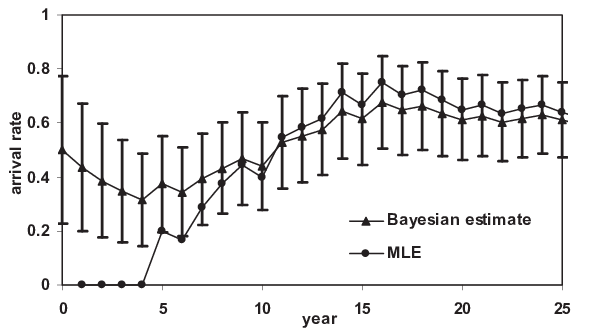
On the same figure, we show the standard maximum likelihood estimate of the arrival rate $\widehat{\lambda}_{k}^{\mbox{\tiny{MLE}}}=\textstyle{1\over k}\sum\nolimits_{i=1}^{k}{n_{i}}$ . After approximately 8 years, the estimators are very close to each other. However, for a small number of observed years, the Bayesian estimate is more accurate as it takes the prior information into account. Only after 12 years do both estimators converge to the true value of 0.6 (this is because the bank was very lucky to have no events during the first four years). Note that for this example we assumed the prior distribution with a mean equal to 0.5, which is different from the true arrival rate. Thus this example shows that an initially incorrect prior estimator is corrected by the observations as they become available. It is interesting to observe that, in year 14, the estimators become slightly different again. This is because the bank was unlucky to experience event counts (1, 1, 2) in the years (12, 13, 14). As a result, the maximum likelihood estimate becomes higher than the true value, while the Bayesian estimate is more stable (smooth) with respect to the unlucky years. If this example is repeated with different sequences of random numbers, then one would observe quite different maximum likelihood estimates (for small $k)$ and more stable Bayesian estimates.

Finally we note that the standard deviation of the posterior distribution $Gamma(\alpha_{k},\beta_{k})$ is large for small $k$ . It is indicated by the error bars in Figure 2 and calculated as $\beta_{k}\sqrt{\alpha_{k}}$ .

4.7 The Lognormal $\mathcal{LN}(\mu,\sigma)$ Severity

Assume that the loss severity for a risk in one bank is modelled as a random variable from a lognormal distribution, $\mathcal{LN}(\mu,\sigma)$ , whose density is

f(x|\mu,\sigma)=\frac{1}{x\sqrt{2\pi\sigma^{2}}}\exp\left({-\frac{(\ln x-\mu)^{2}}{2\sigma^{2}}}\right).

(25)

This distribution often gives a good fit for operational loss data. Also, it belongs to a class of heavy-tailed (subexponential) distributions. The parameters $\mu$ and $\sigma$ are not known and the Bayesian approach models these as a random variables $\Theta_{\mu}$ and $\Theta_{\sigma}$ respectively. We assume that the losses over the years $t=1,2,\ldots,T$ are observed and should be modelled for next year $T+1$ . To simplify notation, we denote the losses over past $T$ years as $X_{1},\ldots,X_{n}$ and the future losses are $X_{n+1},\ldots\;$ . Then the model can be structured as follows. For simplicity, assume that $\sigma$ is known and $\mu$ is unknown. The case where both $\sigma$ and $\mu$ are unknown can be found in Shevchenko [34, section 4.3.5].

Model Assumptions 4.4

•

Suppose that, given $\sigma$ and $\Theta_{\mu}=\mu$ , the data $X_{1},\ldots,X_{n},\ldots$ are independent random variables from $\mathcal{LN}(\mu,\sigma)$ . That is, $Y_{i}=\ln X_{i}$ , $i=1,2,\ldots$ are distributed from the normal distribution $\mathcal{N}(\mu,\sigma)$ .
•

Assume that parameter $\sigma$ is known and the prior distribution for $\Theta_{\mu}$ is the normal distribution, $\mathcal{N}(\mu_{0},\sigma_{0})$ . That is the prior density is

$\pi(\mu)=\frac{1}{\sigma_{0}\sqrt{2\pi}}\exp\left({-\frac{(\mu-\mu_{0})^{2}}{2\sigma_{0}^{2}}}\right).$ (26)

Denote the losses over past years as ${\bm{X}}=(X_{1},\ldots,X_{n})^{\prime}$ and corresponding log-losses as ${\bm{Y}}=(Y_{1},\ldots,Y_{n})^{\prime}$ . Note that $\mu$ plays the role of ${\bm{\theta}}$ in (10).

Posterior. Under the above assumptions, the joint density of the data over past years (conditional on $\sigma$ and $\Theta_{\mu}=\mu$ ) at position $\bm{Y}=\bm{y}$ is

h({\bm{y}}|\mu,\sigma)=\prod\limits_{i=1}^{n}{\frac{1}{\sigma\sqrt{2\pi}}\exp\left({-\frac{(y_{i}-\mu)^{2}}{2\sigma^{2}}}\right)}.

(27)

Then, using formula (10), the posterior density can be written as

	$\displaystyle\pi(\mu\|{\bm{y}})$	$\displaystyle\propto$	$\displaystyle\frac{\exp\left({-\frac{(\mu-\mu_{0})^{2}}{2\sigma_{0}^{2}}}\right)}{\sigma_{0}\sqrt{2\pi}}\prod\limits_{i=1}^{n}{\frac{\exp\left({-\frac{(y_{i}-\mu)^{2}}{2\sigma^{2}}}\right)}{\sigma\sqrt{2\pi}}}$		(28)
		$\displaystyle\propto$	$\displaystyle\exp\left({-\frac{(\mu-{\mu}_{0,n})^{2}}{2{\sigma}_{0,n}^{2}}}\right),$		(28)

that corresponds to a normal distribution, $\mathcal{N}({\mu}_{0,n},{\sigma}_{0,n})$ , i.e. the same as the prior distribution with updated parameters

	$\displaystyle\mu_{0}\to{\mu}_{0,n}$	$\displaystyle=$	$\displaystyle\frac{\mu_{0}+\omega\sum\limits_{i=1}^{n}{y_{i}}}{1+n\times\omega},$		(29)
	$\displaystyle\sigma_{0}^{2}\to{\sigma}_{0,n}^{2}$	$\displaystyle=$	$\displaystyle\frac{\sigma_{0}^{2}}{1+n\times\omega},\hskip 10.00002pt\mbox{where}\;\;\omega=\sigma_{0}^{2}/\sigma^{2}.$		(30)

The expected value of $Y_{n+1}$ (given past observations), $\mathrm{E}[Y_{n+1}|{\bm{Y}}=\bm{y}]$ , allows for a good interpretation, as follows:

	$\displaystyle\mathrm{E}[Y_{n+1}\|{\bm{Y}}=\bm{y}]=\mathrm{E}[\Theta_{\mu}\|{\bm{Y}}=\bm{y}]={\mu}_{0,n}$	$\displaystyle=$	$\displaystyle\frac{\mu_{0}+\omega\sum\limits_{i=1}^{n}{y_{i}}}{1+n\times\omega}$		(31)
		$\displaystyle=$	$\displaystyle w_{n}\overline{y}_{n}+(1-w_{n})\mu_{0},$		(31)

where

•

$\overline{y}_{n}=\frac{1}{n}\sum\limits_{i=1}^{n}{y_{i}}$ is the estimate of $\mu$ using the observed losses only;
•

$\mu_{0}$ is the estimate of $\mu$ using a prior distribution only (e.g. specified by expert);
•

$w_{n}=\frac{n}{n+\sigma^{2}/\sigma_{0}^{2}}$ is the credibility weight in [0,1) used to combine $\mu_{0}$ and $\overline{y}_{n}$ .

Remarks 4.5

•

As the number of observations increases, the credibility weight $w$ increases and vice versa. That is, the more observations we have the greater weight we assign to the estimator based on the observed counts and the lesser weight is attached to the expert opinion estimate. Also, larger uncertainty in the expert opinion $\sigma_{0}^{2}$ leads to a higher credibility weight for observations and larger volatility of observations $\sigma^{2}$ leads to a higher credibility weight for expert opinions.

•

The posterior distribution can be calculated recursively as follows. Consider the data $Y_{1},Y_{2},\ldots,Y_{k},\ldots$ . Assume that the prior distribution, $\mathcal{N}(\mu_{0},\sigma_{0})$ , is specified initially, then the posterior density ${\pi}(\mu|y_{1},\ldots,y_{k})$ after the $k$ -th event is the normal distribution $\mathcal{N}({\mu}_{0,k},{\sigma}_{0,k})$ with

{\mu}_{0,k}=\frac{\mu_{0}+\omega\sum\limits_{i=1}^{k}{y_{i}}}{1+k\times\omega},\hskip 10.00002pt{\sigma}_{0,k}^{2}=\frac{\sigma_{0}^{2}}{1+k\times\omega},

where $\omega=\sigma_{0}^{2}/\sigma^{2}$ . It is easy to show that

{\mu}_{0,k}=\frac{{\mu}_{0,k-1}+\omega_{k-1}y_{k}}{1+\omega_{k-1}},\;\hskip 10.00002pt{\sigma}_{0,k}^{2}=\frac{\sigma^{2}\omega_{k-1}}{1+\omega_{k-1}}

(32)

with $\omega_{k-1}={\sigma}_{0,k-1}^{2}/\sigma^{2}$ . That is, calculation of the posterior distribution parameters can be based on the most recent observation and the parameters of the posterior distribution calculated just before this observation.

•

Estimation of prior for the parameters of lognormal distribution is considered in Shevchenko and Wüthrich [35].

5 Bayesian Method to Combine Three Data Sources

In the previous section we showed how to combine two data sources: expert opinions and internal data; or external data and internal data. In order to estimate the risk capital of a bank and to fulfill the Basel II requirements, risk managers have to take into account internal data, relevant external data (industry data) and expert opinions. The aim of this section is to provide an example of methodology to be used to combine these three sources of information. Here, we follow the approach suggested in Lambrigger et al [36]. As in the previous section, we consider one risk cell only. In terms of methodology we go through the following steps:

•

In any risk cell, we model the loss frequency and the loss severity by parametric distributions (e.g. Poisson for the frequency or Pareto, lognormal, etc. for the severity). For the considered bank, the unknown parameter vector $\bm{\theta}$ (for example, the Poisson parameter or the Pareto tail index) of these distributions has to be quantified.
•

A priori, before we have any company specific information, only industry data are available. Hence, the best prediction of our bank specific parameter $\bm{\theta}$ is given by the belief in the available external knowledge such as the provided industry data. This unknown parameter of interest is modelled by a prior distribution (structural distribution) corresponding to a random vector $\bm{\Theta}$ . The parameters of the prior distribution (hyper-parameters) are estimated using data from the whole industry by, for example, maximum likelihood estimation. If no industry data are available, the prior distribution could come from a “super expert” that has an overview over all banks.
•

The true bank specific parameter $\bm{\theta}_{0}$ is treated as a realisation of $\bm{\Theta}$ . The prior distribution of a random vector $\bm{\Theta}$ corresponds to the whole banking industry sector, whereas $\bm{\theta}$ stands for the unknown underlying parameter set of the bank being considered. Due to the variability amongst banks, it is natural to model $\bm{\theta}$ by a probability distribution. Note that $\bm{\Theta}$ is random with known distribution, whereas $\bm{\theta}_{0}$ is deterministic but unknown.
•

As time passes, internal data $\bm{X}=(X_{1},\ldots,X_{K})^{\prime}$ as well as expert opinions $\bm{\Delta}=(\Delta_{1},\ldots,\Delta_{M})^{\prime}$ about the underlying parameter $\bm{\theta}$ become available. This affects our belief in the distribution of $\bm{\Theta}$ coming from external data only and adjust the prediction of $\bm{\theta}_{0}$ . The more information on $\bm{X}$ and $\bm{\Delta}$ we have, the better we are able to predict $\bm{\theta}_{0}$ . That is, we replace the prior density $\pi(\bm{\theta})$ by a conditional density of $\bm{\Theta}$ given $\bm{X}$ and $\bm{\Delta}$ .

In order to determine the posterior density $\pi(\bm{\theta}|\bm{x},\bm{\delta})$ , consider the joint conditional density of observations and expert opinions (given the parameter vector $\bm{\theta}$ ):

h(\bm{x},\bm{\delta}|\bm{\theta})=h_{1}(\bm{x}|\bm{\theta})h_{2}(\bm{\delta}|\bm{\theta}),

(33)

where $h_{1}$ and $h_{2}$ are the conditional densities (given $\bm{\Theta}=\bm{\theta}$ ) of $\bm{X}$ and $\bm{\Delta}$ , respectively. Thus $\bm{X}$ and $\bm{\Delta}$ are assumed to be conditionally independent given $\bm{\Theta}$ .

Remarks 5.1

•

Notice that, in this way, we naturally combine external data information, $\pi(\bm{\theta})$ , with internal data $\bm{X}$ and expert opinion $\bm{\Delta}$ .
•

In classical Bayesian inference (as it is used, for example, in actuarial science), one usually combines only two sources of information as described in the previous sections. Here, we combine three sources simultaneously using an appropriate structure, that is, equation (33).
•

Equation (33) is quite a reasonable assumption. Assume that the true bank specific parameter is $\bm{\theta}_{0}$ . Then, (33) says that the experts in this bank estimate $\bm{\theta}_{0}$ (by their opinion $\bm{\Delta}$ ) independently of the internal observations. This makes sense if the experts specify their opinions regardless of the data observed. Otherwise we should work with the joint distribution $h(\bm{x},\bm{\delta}|\bm{\theta})$ .

We further assume that observations as well as expert opinions are conditionally independent and identically distributed, given $\bm{\Theta}=\bm{\theta}$ , so that

	$\displaystyle h_{1}(\bm{x}\|\bm{\theta})$	$\displaystyle=$	$\displaystyle\prod_{k=1}^{K}f_{1}(x_{k}\|\bm{\theta}),$		(34)
	$\displaystyle h_{2}(\bm{\delta}\|\bm{\theta})$	$\displaystyle=$	$\displaystyle\prod_{m=1}^{M}f_{2}(\delta_{m}\|\bm{\theta}),$		(35)

where $f_{1}$ and $f_{2}$ are the marginal densities of a single observation and a single expert opinion, respectively. We have assumed that all expert opinions are identically distributed, but this can be generalised easily to expert opinions having different distributions.

Here, the unconditional parameter density $\pi(\bm{\theta})$ is the prior density, whereas the conditional parameter density $\pi(\bm{\theta}|\bm{x},\bm{\delta})$ is the posterior density. Let $h(\bm{x},\bm{\delta})$ denote the unconditional joint density of the data $\bm{X}$ and expert opinions $\bm{\Delta}$ . Then, it follows from Bayes’s theorem that

h(\bm{x},\bm{\delta}|\bm{\theta})\pi(\bm{\theta})=\pi(\bm{\theta}|\bm{x},\bm{\delta})h(\bm{x},\bm{\delta}).

(36)

Note that the unconditional density $h(\bm{x},\bm{\delta})$ does not depend on $\bm{\theta}$ and thus the posterior density is given by

\pi(\bm{\theta}|\bm{x},\bm{\delta})\propto\pi(\bm{\theta})\prod_{k=1}^{K}f_{1}(x_{k}|\bm{\theta})\prod_{m=1}^{M}f_{2}(\delta_{m}|\bm{\theta}).

(37)

For the purposes of OpRisk, it should be used to estimate the predictive distribution of future losses.

5.1 Modelling Frequency: Poisson Model

To model the loss frequency for OpRisk in a risk cell, consider the following model.

Model Assumptions 5.2 (Poisson-gamma-gamma)

Assume that a risk cell in a bank has a scaling factor $V$ for the frequency in a specified risk cell (it can be the product of several economic factors such as the gross income, the number of transactions or the number of staff).

a)

Let $\Lambda\sim Gamma(\alpha_{0},\beta_{0})$ be a gamma distributed random variable with shape parameter $\alpha_{0}>0$ and scale parameter $\beta_{0}>0$ , which are estimated from (external) market data. That is, the density of $Gamma(\alpha_{0},\beta_{0})$ , plays the role of $\pi(\bm{\theta})$ in (37).
b)

Given $\Lambda=\lambda$ , the annual frequencies, $N_{1},\ldots,N_{T},N_{T+1}$ , where $T+1$ refers to next year, are assumed to be independent and identically distributed with $N_{t}\sim Poisson(V\lambda)$ . That is, $f_{1}(\cdot|\lambda)$ in (37) corresponds to the probability mass function of a $Poisson(V\lambda)$ distribution.
c)

A financial company has $M$ expert opinions $\Delta_{m}$ , $1\leq m\leq M$ , about the intensity parameter $\Lambda$ . Given $\Lambda=\lambda$ , $\Delta_{m}$ and $N_{t}$ are independent for all $t$ and $m$ , and $\Delta_{1},\ldots,\Delta_{M}$ are independent and identically distributed with $\Delta_{m}\sim Gamma(\xi,\lambda/\xi)$ , where $\xi$ is a known parameter. That is, $f_{2}(\cdot|\lambda)$ corresponds to the density of a $Gamma(\xi,\lambda/\xi)$ distribution.

Remarks 5.3

•

The parameters $\alpha_{0}$ and $\beta_{0}$ in Model Assumptions 5.2 are hyper-parameters (parameters for parameters) and can be estimated using the maximum likelihood method or the method of moments.
•

In Model Assumptions 5.2 we assume

$\mathrm{E}[\Delta_{m}|\Lambda]=\Lambda,\hskip 10.00002pt1\leq m\leq M,$ (38)

that is, expert opinions are unbiased. A possible bias might only be recognised by the regulator, as he alone has the overview of the whole market.

Note that the coefficient of variation of the conditional expert opinion $\Delta_{m}|\Lambda$ is

\mathrm{Vco}[\Delta_{m}|\Lambda]=(\mathrm{Var}[\Delta_{m}|\Lambda)])^{1/2}/\mathrm{E}[\Delta_{m}|\Lambda]=1/\sqrt{\xi},

and thus is independent of $\Lambda$ . This means that $\xi$ , which characterises the uncertainty in the expert opinions, is independent of the true bank specific $\Lambda$ . For simplicity, we have assumed that all experts have the same conditional coefficient of variation and thus have the same credibility. Moreover, this allows for the estimation of $\xi$ as

\widehat{\xi}=(\widehat{\mu}/\widehat{\sigma})^{2},

(39)

where

\widehat{\mu}=\frac{1}{M}\sum_{m=1}^{M}\delta_{m}\hskip 10.00002pt\textnormal{and}\hskip 10.00002pt\widehat{\sigma}^{2}=\frac{1}{M-1}\sum_{m=1}^{M}(\delta_{m}-\widehat{\mu})^{2},\hskip 10.00002ptM\geq 2.

In a more general framework the parameter $\xi$ can be estimated, for example, by maximum likelihood.

In the insurance practice $\xi$ is often specified by the regulator denoting a lower bound for expert opinion uncertainty; e.g. Swiss Solvency Test, see Swiss Financial Market Supervisory Authority ([37], appendix 8.4). If the credibility differs among the experts, then $\mathrm{Vco}[\Delta_{m}|\Lambda]$ should be estimated for all $m$ , $1\leq m\leq M$ . Admittedly, this may often be a challenging issue in practice.

Remarks 5.4

This model can be extended to a model where one allows for more flexibility in the expert opinions. For convenience, it is preferred that experts are conditionally independent and identically distributed, given $\Lambda$ . This has the advantage that there is only one parameter, $\xi$ , that needs to be estimated.

Using the notation from Section 5, the posterior density of $\Lambda$ , given the losses up to year $K$ and the expert opinions of $M$ experts, can be calculated. Denote the data over past years as follows:

	$\displaystyle\bm{N}$	$\displaystyle=$	$\displaystyle(N_{1},\ldots,N_{T})^{\prime},$
	$\displaystyle\bm{\Delta}$	$\displaystyle=$	$\displaystyle(\Delta_{1},\ldots,\Delta_{M})^{\prime}.$

Also, denote the arithmetic means by

\overline{N}=\frac{1}{T}\sum_{t=1}^{T}N_{t},\hskip 10.00002pt\overline{\Delta}=\frac{1}{M}\sum_{m=1}^{M}\Delta_{m},\hskip 10.00002pt\textnormal{etc.}

(40)

Then, the posterior density is given by the following theorem.

Theorem 5.1

Under Model Assumptions 5.2, given loss information $\bm{N}=\bm{n}$ and expert opinion $\bm{\Delta}=\bm{\delta}$ , the posterior density of $\Lambda$ is

\pi(\lambda|\bm{n},\bm{\delta})=\frac{(\omega/\phi)^{(\nu+1)/2}}{2K_{\nu+1}(2\sqrt{\omega\phi})}\lambda^{\nu}e^{-\lambda\omega-\lambda^{-1}\phi},

(41)

with

$\displaystyle\nu$	$\displaystyle=$	$\displaystyle\alpha_{0}-1-M\xi+T\overline{n},$
$\displaystyle\omega$	$\displaystyle=$	$\displaystyle VT+\frac{1}{\beta_{0}},$	(42)
$\displaystyle\phi$	$\displaystyle=$	$\displaystyle\xi M\overline{\delta},$

and

K_{\nu+1}(z)=\frac{1}{2}\int_{0}^{\infty}u^{\nu}e^{-z(u+1/u)/2}\textnormal{d}u.

(43)

Here, $K_{\nu}(z)$ is a modified Bessel function of the third kind; see for instance Abramowitz and Stegun ([38], p. 375).

Proof 5.5

Model Assumptions 5.2 applied to (37) yield

$\displaystyle{\pi}(\lambda\|\bm{n},\bm{\delta})$	$\displaystyle\propto$	$\displaystyle\lambda^{\alpha_{0}-1}e^{-\lambda/\beta_{0}}\prod_{t=1}^{T}e^{-V\lambda}\frac{(V\lambda)^{n_{t}}}{n_{t}!}\prod_{m=1}^{M}\frac{(\delta_{m})^{\xi-1}}{(\lambda/\xi)^{\xi}}e^{-\delta_{m}\xi/\lambda}$
	$\displaystyle\propto$	$\displaystyle\lambda^{\alpha_{0}-1}e^{-\lambda/\beta_{0}}\prod_{t=1}^{T}e^{-V\lambda}\lambda^{n_{t}}\prod_{m=1}^{M}(\xi/\lambda)^{\xi}e^{-\delta_{m}\xi/\lambda}$
	$\displaystyle\propto$	$\displaystyle\lambda^{\alpha_{0}-1-M\xi+T\overline{n}}\exp{\left(-\lambda\left(VT+\frac{1}{\beta_{0}}\right)-\frac{1}{\lambda}\xi M\overline{\delta}\right)}.$

Remarks 5.6

•

A distribution with density (41) is known as the generalised inverse Gaussian distribution GIG $(\omega,\phi,\nu)$ . This is a well-known distribution with many applications in finance and risk management; see McNeil et al [6, p. 75 and p. 497].
•

In comparison with the classical Poisson-gamma case of combining two sources of information (considered in Section 4.5), where the posterior is a gamma distribution, the posterior $\pi(\lambda|\cdot)$ in (5.5) is more complicated. In the exponent, it involves both $\lambda$ and $1/\lambda$ . Note that expert opinions enter via the term $1/\lambda$ only.
•

Observe that the classical exponential dispersion family with associated conjugates (see Chapter 2.5 in Bühlmann and Gisler [32]) allows for a natural extension to GIG-like distributions. In this sense the GIG distributions enlarge the classical Bayesian inference theory on the exponential dispersion family.

For our purposes it is interesting to observe how the posterior density transforms when new data from a newly observed year arrive. Let $\nu_{k}$ , $\omega_{k}$ and $\phi_{k}$ denote the parameters for the data $(N_{1},\ldots,N_{k})$ after $k$ accounting years. Implementation of the update processes is then given by the following equalities (assuming that expert opinions do not change).

$\displaystyle\nu_{k+1}$	$\displaystyle=$	$\displaystyle\nu_{k}+n_{k+1},$
$\displaystyle\omega_{k+1}$	$\displaystyle=$	$\displaystyle\omega_{k}+V,$	(44)
$\displaystyle\phi_{k+1}$	$\displaystyle=$	$\displaystyle\phi_{k}.$

Obviously, the information update process has a very simple form and only the parameter $\nu$ is affected by the new observation $n_{k+1}$ . The posterior density (5.5) does not change its type every time new data arrive and hence, is easily calculated.

The moments of a GIG are not available in a closed form through elementary functions but can be expressed in terms of Bessel functions. In particular, the posterior expected number of losses is

\mathrm{E}[\Lambda|\bm{N}=\bm{n},\bm{\Delta}=\bm{\delta}]=\sqrt{\frac{\phi}{\omega}}\frac{K_{\nu+2}(2\sqrt{\omega\phi})}{K_{\nu+1}(2\sqrt{\omega\phi})}.

(45)

The mode of a GIG has a simple expression that gives the posterior mode

\textnormal{mode}(\Lambda|\bm{N}=\bm{n},\bm{\Delta}=\bm{\delta})=\frac{1}{2\omega}(\nu+\sqrt{\nu^{2}+4\omega\phi}).

(46)

It can be used as an alternative point estimator instead of the mean. Also, the mode of a GIG differs only slightly from the expected value for large $|\nu|$ . A full asymptotic interpretation of the Bayesian estimator (45) can be found Lambrigger et al [36] that shows the model behaves as we would expect and require in practice.

5.2 Numerical example

A simple example, taken from Lambrigger et al [36, example 3.7], illustrates the above methodology combining three data sources. It also extends numerical example from Section 4.6, where two data sources are combined using classical Bayesian inference approach. Assume that:

•

External data (for example, provided by external databases or regulator) estimate the intensity of the loss frequency (i.e. the Poisson parameter $\Lambda$ ), which has a prior gamma distribution $\Lambda\sim Gamma(\alpha_{0},\beta_{0})$ , as $\mathrm{E}[\Lambda]=\alpha_{0}\beta_{0}=0.5$ and $\Pr[0.25\leq\Lambda\leq 0.75]=2/3$ . Then, the parameters of the prior are $\alpha_{0}\approx 3.407$ and $\beta_{0}\approx 0.147$ ; see Section 4.6.
•

One expert gives an estimate of the intensity as $\delta=0.7$ . For simplicity, we consider in this example one single expert only and hence, the coefficient of variation is not estimated using (39), but given a priori (e.g. by the regulator): $\mathrm{Vco}[\Delta|\Lambda]=\sqrt{\mathrm{Var}[\Delta|\Lambda]}/\mathrm{E}[\Delta|\Lambda]=0.5$ , i.e. $\xi=4$ .
•

The observations of the annual number of losses $n_{1},n_{2},\ldots$ are sampled from $Poisson(0.6)$ and are the same as in Section 4.6.

This means that a priori we have a frequency parameter distributed as $Gamma(\alpha_{0},\beta_{0})$ with mean $\alpha_{0}\beta_{0}=0.5$ . The true value of the parameter $\lambda$ for this risk in a bank is $0.6$ , that is, it does worse than the average institution. However, our expert has an even worse opinion of his institution, namely $\delta=0.7$ . Now, we compare:

•

the pure maximum likelihood estimate $\widehat{\lambda}_{k}^{\mbox{\tiny{MLE}}}=\frac{1}{k}\sum_{i=1}^{k}n_{i};$
•

the Bayesian estimate (22), $\widehat{\lambda}_{k}^{(2)}=\mathrm{E}[\Lambda|N_{1}=n_{1},\ldots,N_{k}=n_{k}]$ , without expert opinion;
•

the Bayesian estimate derived in formula (45) $\widehat{\lambda}_{k}^{(3)}=\mathrm{E}[\Lambda|N_{1}=n_{1},\ldots,N_{k}=n_{k},\Delta=\delta]$ , that combines internal data and expert opinions with the prior.

The results are plotted in Figure 3. The estimator $\widehat{\lambda}_{k}^{(3)}$ shows a much more stable behaviour around the true value $\lambda=0.6$ , due to the use of the prior information (market data) and the expert opinions. Given adequate expert opinions, $\widehat{\lambda}_{k}^{(3)}$ clearly outperforms the other estimators, particularly if only a few data points are available.

One could think that this is only the case when the experts’ estimates are appropriate. However, even if experts fairly under- (or over-) estimate the true parameter $\lambda$ , the method presented here performs better for our dataset than the other mentioned methods, when a few data points are available. The above example yields a typical picture observed in numerical experiments that demonstrates that the Bayes estimator (45) is often more suitable and stable than maximum likelihood estimators based on internal data only. Note that in this example the prior distribution as well as the expert opinion do not change over time. However, as soon as new information is available or when new risk management tools are in place, the corresponding parameters may be easily adjusted.

Remarks 5.7

In this section, we considered the situation where ${\Lambda}$ is the same for all years $t=1,2,\ldots$ . However, in general, the evolution of ${\Lambda}_{t}$ , can be modelled as having deterministic (trend, seasonality) and stochastic components, the case when ${\Lambda}_{t}$ is purely stochastic and distributed according to a gamma distribution is considered in Peters, et al [39].

5.3 Lognormal Model for Severities

In general, one can use the methodology summarised by equation (37) to develop a model combining external data, internal data and expert opinion for estimation of the severity. For illustration purposes, this section considers the lognormal severity model.

Consider modelling severities $X_{1},\ldots,X_{K},\ldots\;$ using the lognormal distribution $\mathcal{LN}(\mu,\sigma)$ , where $\bm{X}=(X_{1},\ldots,X_{K})^{\prime}$ are the losses over past $T$ years. Here, we take an approach considered in Section 4.7, where $\mu$ is unknown and $\sigma$ is known. The unknown $\mu$ is treated under the Bayesian approach as a random variable $\Theta_{\mu}$ . Then combining external data, internal data and expert opinions can be accomplished using the following model.

Model Assumptions 5.8 (Lognormal-normal-normal)

Let us assume the following severity model for a risk cell in one bank:

a)

Let $\Theta_{\mu}\sim\mathcal{N}(\mu_{0},\sigma_{0})$ be a normally distributed random variable with parameters $\mu_{0},\sigma_{0}$ , which are estimated from (external) market data, i.e. $\pi(\bm{\theta})$ in (37) is the density of $\mathcal{N}(\mu_{0},\sigma_{0})$ .
b)

Given $\Theta_{\mu}=\mu$ , the losses $X_{1},X_{2},\ldots\;$ are conditionally independent with a common lognormal distribution: $X_{k}{\sim}\mathcal{LN}(\mu,\sigma)$ , where $\sigma$ is assumed known. That is, $f_{1}(\cdot|\mu)$ in (37) corresponds to the density of a $\mathcal{LN}(\mu,\sigma)$ distribution.
c)

The financial company has $M$ experts with opinions $\Delta_{m}$ , $1\leq m\leq M$ , about $\Theta_{\mu}$ . Given $\Theta_{\mu}=\mu$ , $\Delta_{m}$ and $X_{k}$ are independent for all $m$ and $k$ , and $\Delta_{1},\ldots,\Delta_{M}$ are independent with a common normal distribution: $\Delta_{m}{\sim}\mathcal{N}(\mu,\xi)$ , where $\xi$ is a parameter estimated using expert opinion data. That is, $f_{2}(\cdot|\mu)$ corresponds to the density of a $\mathcal{N}(\mu,\xi)$ distribution.

Remarks 5.9

•

For $M\geq 2$ , the parameter $\xi$ can be estimated by the standard deviation of $\delta_{m}$ :

$\widehat{\xi}=\left(\frac{1}{M-1}\sum_{m=1}^{M}(\delta_{m}-\overline{\delta})^{2}\right)^{1/2}.$ (47)
•

The hyper-parameters $\mu_{0}$ and $\sigma_{0}$ are estimated from market data, for example, by maximum likelihood estimation or by the method of moments.
•

In practice one often uses an ad-hoc estimate for $\sigma$ , which usually is based on expert opinion only. However, one could think of a Bayesian approach for $\sigma$ , but then an analytical formula for the posterior distribution in general does not exist and the posterior needs then to be calculated numerically, for example, by MCMC methods.

Under Model Assumptions 5.8, the posterior density is given by

$\displaystyle{\pi}(\mu\|\bm{x},\bm{\delta})$	$\displaystyle\propto$	$\displaystyle\frac{1}{\sigma_{0}\sqrt{2\pi}}\exp\left(-\frac{(\mu-\mu_{0})^{2}}{2\sigma_{0}^{2}}\right)\prod_{k=1}^{K}\frac{1}{\sigma\sqrt{2\pi}}\exp\left(-\frac{(\ln x_{k}-\mu)^{2}}{2\sigma^{2}}\right)$	(48)
		$\displaystyle\prod_{m=1}^{M}\frac{1}{\xi\sqrt{2\pi}}\exp\left(-\frac{(\delta_{m}-\mu)^{2}}{2\xi^{2}}\right)$
	$\displaystyle\propto$	$\displaystyle\exp\left[-\left(\frac{(\mu-\mu_{0})^{2}}{2\sigma_{0}^{2}}+\sum_{k=1}^{K}\frac{(\ln x_{k}-\mu)^{2}}{2\sigma^{2}}+\sum_{m=1}^{M}\frac{(\delta_{m}-\mu)^{2}}{2\xi^{2}}\right)\right]$
	$\displaystyle\propto$	$\displaystyle\exp\left[-\frac{(\mu-\widehat{\mu})^{2}}{2\widehat{\sigma}^{2}}\right],$

with

\widehat{\sigma}^{2}=\left(\frac{1}{\sigma_{0}^{2}}+\frac{K}{\sigma^{2}}+\frac{M}{\xi^{2}}\right)^{-1},

and

\widehat{\mu}=\widehat{\sigma}^{2}\times\left(\frac{\mu_{0}}{\sigma_{0}^{2}}+\frac{1}{\sigma^{2}}\sum_{k=1}^{K}\ln x_{k}+\frac{1}{\xi^{2}}\sum_{m=1}^{M}\delta_{m}\right).

In summary, we derived the following theorem (also see Lambrigger et al [36]). That is, the posterior distribution of $\Theta_{\mu}$ , given loss information $\bm{X}=\bm{x}$ and expert opinion $\bm{\Delta}=\bm{\delta}$ , is a normal distribution $\mathcal{N}(\widehat{\mu},\widehat{\sigma})$ with

\widehat{\sigma}^{2}=\left(\frac{1}{\sigma_{0}^{2}}+\frac{K}{\sigma^{2}}+\frac{M}{\xi^{2}}\right)^{-1}

and

\widehat{\mu}=\mathrm{E}[\Theta_{\mu}|\bm{X}=\bm{x},\bm{\Delta}=\bm{\delta}]=\omega_{1}\mu_{0}+\omega_{2}\overline{\ln x}+\omega_{3}\overline{\delta},

(49)

where $\overline{\ln x}=\frac{1}{K}\sum_{k=1}^{K}\ln x_{k}$ and the credibility weights are

\omega_{1}=\widehat{\sigma}^{2}/\sigma_{0}^{2},\;\omega_{2}=\widehat{\sigma}^{2}K/\sigma^{2},\;\omega_{3}=\widehat{\sigma}^{2}M/\xi^{2}.

This yields a natural interpretation. The more credible the information, the higher is the credibility weight in (49) – as expected from an appropriate model for combining internal observations, relevant external data and expert opinions.

6 Nonparametric Bayesian approach

Typically, under the Bayesian approach, we assume that there is unknown distribution underlying observations $x_{1},\ldots,x_{n}$ and this distribution is parametrized by $\bm{\theta}$ . Then we place a prior distribution on the parameter $\bm{\theta}$ and try to infer the posterior of $\bm{\theta}$ given observations $x_{1},\ldots,x_{n}$ . Under the nonparametric approach, we do not make assumption that underlying loss process generating distribution is parametric; we put prior on the distribution directly and find the posterior of the distribution given data which is combining of the prior with empirical data distribution.

One of the most popular Bayesian nonparametric models is based on Dirichlet process introduced in Ferguson [40]. The Dirichlet process represents a probability distribution of the probability distributions. It can be specified in terms of a base distribution $H(x)$ and a scalar concentration parameter $\alpha>0$ and denoted as $DP(\alpha,H)$ . For example, assume that we model severity distribution $F(x)$ which is unknown and modelled as random at each point $x$ using $DP(\alpha,H)$ . Then, the mean value of $F(x)$ is the base distribution $H(x)$ and variance of $F(x)$ is $H(x)(1-H(x))/(\alpha+1)$ . That is, as the concentration parameter $\alpha$ increases, the true distribution is getting closer to the base distribution $H(x)$ . Each draw from Dirichlet process is a distribution function and for $x_{1}<x_{2}<\cdots<x_{k}$ , the distribution of

F(x_{1}),F(x_{2})-F(x_{1}),\ldots,1-F(x_{k})

is a $k+1$ multivariate Dirichlet distribution

Dir(\alpha H(x_{1}),\alpha(H(x_{2})-H(x_{1})),\ldots,\alpha(1-H(x_{k})))

formally defined as follows.

Definition 6.1 (Dirichlet distribution)

A d-variate Dirichlet distribution is denoted as $Dir(\alpha_{1},\alpha_{2},\ldots,\alpha_{d})$ , where $\alpha_{i}>0$ . The random vector $(Q_{1},Q_{2},\ldots,Q_{d})$ has a Dirichlet distribution if its density function is

f(q_{1},q_{2},\ldots,q_{d-1})=\frac{\Gamma(\alpha_{1}+\cdots+\alpha_{d})}{\prod_{i=1}^{d}\Gamma(\alpha_{i})}\prod_{i=1}^{d}q_{i}^{\alpha_{i}-1},

(50)

where $q_{i}>0$ and $q_{1}+\cdots+q_{d}=1$ .

There are several formal definitions of Dirichlet processes; for detailed description see Ghosh and Ramamoorthi [41]. For the purposes of this book, here we just present few important results that can be easily adopted for OpRisk. In particular, the $i$ th marginal distribution of $Dir(\alpha_{1},\ldots,\alpha_{d})$ is $Beta(\alpha_{i},\alpha_{0}-\alpha_{i})$ , where $\alpha_{0}=\alpha_{1}+\cdots+\alpha_{d}$ . Thus the marginal distribution of the Dirichlet process $DP(\alpha,H)$ is beta distribution $F(x)\sim Beta(\alpha H(x),\alpha(1-H(x)))$ , i.e. explicitly it has the Beta density

\Pr[F(x)\in dy]=\frac{\Gamma(\alpha)}{\Gamma(\alpha H(x))\Gamma(\alpha(1-H(x)))}y^{\alpha H(x)}(1-y)^{\alpha(1-H(x))-1}dy,

(51)

where $\Gamma(\cdot)$ is a gamma function.

If the prior distribution for $F(x)$ is $DP(\alpha,H)$ , then after observing $x_{1},\ldots,x_{n}$ , the posterior for $F(x)$ is

DP\left(\alpha+n,\frac{\alpha}{\alpha+n}H(x)+\frac{n}{\alpha+n}\frac{1}{n}\sum 1_{x_{i}\leq x}\right).

(52)

In other words, Dirichlet process is a conjugate prior with respect to empirical sample distribution; in posterior, our unknown distribution $F(x)$ will have updated concentration parameter $\alpha+n$ and updated base distribution

\widetilde{H}(x)=\frac{\alpha}{\alpha+n}H(x)+\frac{n}{\alpha+n}\frac{1}{n}\sum 1_{x_{i}\leq x},

(53)

which is a weighted sum of the prior base distribution and empirical distribution with the weights ${\alpha}/(\alpha+n)$ and $n/(\alpha+n)$ respectively. The modeller can choose $H(x)$ as an expert opinion on distribution $F(x)$ , then posterior estimate of the $F(x)$ after observing data $x_{1},\ldots,x_{n}$ will be given by $\widetilde{H}(x)$ in (53).

Remarks 6.2

•

As new data are collected, the posterior distribution converges to the empirical distribution that itself converges to the true distribution of $F(x)$ .
•

The larger value of $\alpha$ , the less impact new data will have on the posterior estimate of $F(x)$ ; if $\alpha=0$ , the posterior distribution will simply be the empirical distribution of the data.
•

The concentration parameter $\alpha$ can be interpreted as an“effective sample size� associated with the prior estimate. In assigning the value of c, the modeler should attempt to quantify the level of information contained in the scenario estimates, as measured by the equivalent amount of data that would provide a similar level of confidence. The modeller can also estimate $\alpha$ from a likely interval range of severities or frequencies (i.e. from the variance of the possible distribution). Cope [42] suggests that given the rarity of the scenarios considered, the assigned value of $\alpha$ will likely be low, often less than ten and possibly as low as one.

Numerical Example. Assume that expert provides estimates in USD millions for a risk severity as follows. If loss occurs, then the probability to exceed 10, 30, 50 and 120 are 0.9, 0.5, 0.25 and 0.1 respectively, and the maximum possible loss is USD 600 million. That is, probability distribution $H(x)$ at points (0, 10, 30, 50, 120, 600) is (0, 0.1, 0.5, 0.75, 0.9, 1). It is presented in Figure 4 with linear interpolation between specified distribution points. If we choose the prior for the unknown severity distribution $F(x)$ as $DP(\alpha,H(x))$ with concentration parameter $\alpha=10$ , then expected value for $F(x)$ from the prior is $H(x)$ and bounds for $F(x)$ for each $x$ can be calculated from the marginal beta distribution (51). For example, the lower and upper bounds in Figure 4 correspond to 0.1 and 0.9 quantiles of the beta distribution $Beta(\alpha H(x),\alpha(1-H(x)))$ , i.e. will contain the true value of $F(x)$ with probability 0.8 for each $x$ . Now, assume that we observe the actual losses 20, 30, 50, 80, 120, 170, 220, and 280 all in USD million. The posterior mean of $F(x)$ combining scenario and data is easily calculated using (53) and presented in Figure 5 along with the empirical data and scenario distribution.

7 Combining using Dempster-Shafer structures

Often risk assessment includes situations where there is little information on which to evaluate a probability or information is nonspecific, ambiguous, or conflicting. In this case one can work with bounds on probability. For example, this idea has been developed in Walley and Fine [43], Berleant [44] and there are suggestions that the idea has its roots from Boole [45]. Williamson and Downs [46] introduced interval-type bounds on cumulative distribution functions called probability boxes or p-boxes. They also described algorithms to compute arithmetic operations (addition, subtraction, multiplication and division) on pairs of p-boxes.

The method of reasoning with uncertain information known as Dempster-Shafer theory of evidence was suggested in Dempster [47, 48] and Shafer [49]. A special rule to combine the evidence from different sources was formulated in Dempster [48]; it is somewhat controversial and there are many modifications to the rule such as in Yager [50, 51].

For a good summary on the methods for obtaining Dempster-Shafer structures and “p-boxes”, and aggregation methods handling a conflict between the objects from different sources, see Ferson et al [52]. The use of p-boxes and Dempster-Shafer structures in risk analyses offers many significant advantages over a traditional probabilistic approach. Ferson et al [52] lists the following practical problems faced by analysts that can be resolved using these methods: imprecisely specified distributions, poorly known or even unknown dependencies, non-negligible measurement uncertainty, non-detects or other censoring in measurements, small sample size, inconsistency in the quality of input data, model uncertainty, and non-stationarity (non-constant distributions).

It is emphasized in Walley [53] that the use of imprecise probabilities does not require one to assume the actual existence of any underlying distribution function. This approach could be useful in risk analyses even when the underlying stochastic processes are nonstationary or could never, even in principle, be identified to precise distribution functions. Oberkampf et al [54] and Oberkampf [55] demonstrated how the theory could be used to model uncertainty in engineering applications of risk analysis stressing that the use of p-boxes and Dempster-Shafer structures in risk analyses offers many significant advantages over a traditional probabilistic approach.

These features are certainly attractive for OpRisk, especially for combining expert opinions, and were applied for OpRisk in Sakalo and Delasey [56]. At the same time, some writers consider these methods as unnecessary elaboration that can be handled within the Bayesian paradigm through Baysian robustness (section 4.7 in Berger [33]). Also, it might be difficult to justify application of Dempster’s rule (or its other versions) to combine statistical bounds for empirical data distribution with exact bounds for expert opinions.

7.1 Dempster-Shafer structures and p-boxes

A Dempster-Shafer structure on the real line is similar to a discrete distribution except that the locations where the probability mass resides are sets of real values (focal elements) rather than points. The correspondence of probability masses associated with the focal elements is called the basic probability assignment. This is analogous to the probability mass function for an ordinary discrete probability distribution. Unlike a discrete probability distribution on the real line, where the mass is concentrated at distinct points, the focal elements of a Dempster-Shafer structure may overlap one another, and this is the fundamental difference that distinguishes Dempster-Shafer theory from traditional probability theory. Dempster-Shafer theory has been widely studied in computer science and artificial intelligence, but has never achieved complete acceptance among probabilists and traditional statisticians, even though it can be rigorously interpreted as classical probability theory in a topologically coarser space.

Definition 7.1 (Dempster-Shafer structure)

A finite Dempster-Shafer structure on the real line $\mathbb{R}$ is probability assignment, which is a mapping

m:2^{\mathbb{R}}\rightarrow[0;1],

where $m(\emptyset)=0$ ; $m(a_{i})=p_{i}$ for focal elements $a_{i}\subseteq{\mathbb{R}}$ , $i=1,2,\ldots,n$ ; and $m(D)=0$ whenever $D\neq a_{i}$ for all $i$ , such that $0<p_{i}$ and $p_{1}+\cdots+p_{n}=1$ .

For convenience, we will assume that the focal elements $a_{i}$ are closed intervals $[x_{i},y_{i}]$ . Then implementation of a Dempster-Shafer structure will require $3n$ numbers; one for each $p_{i}$ ; and $x_{i}$ and $y_{i}$ for each corresponding focal element.

Remarks 7.2

Note that $2^{\mathbb{R}}$ denotes a power set. The power set of a set $\mathbb{S}$ is the set of all subsets of $\mathbb{S}$ including the empty set $\emptyset$ and $\mathbb{S}$ itself. If $\mathbb{S}$ is a finite set with $K$ elements then the number of elements in its power set is $2^{K}$ . For example, if $\mathbb{S}$ is the set $\{x,y\}$ , then the power set is $\{\emptyset,x,y,\{x,y\}\}$ .

The upper and lower probability bounds can be defined for Dempster-Shafer structure. These are called plausibility and belief functions defined as follows.

Definition 7.3 (Plausibility function)

The plausibility function corresponding to a Dempster-Shafer structure $m(A)$ is the sum of all masses associated with sets that overlap with or merely touch the set $b\subseteq{\mathbb{R}}$

Pls(b)=\sum_{a_{i}\cap b\neq\emptyset}m(a_{i}),

which is the sum over $i$ such that $a_{i}\cap b\neq\emptyset$ .

Definition 7.4 (Belief function)

The belief function corresponding to a Dempster-Shafer structure $m(A)$ is the sum of all masses associated with sets that are subsets of $b\subseteq{\mathbb{R}}$

Bel(b)=\sum_{a_{i}\subseteq b}m(a_{i}),

which is the sum over $i$ such that $a_{i}\subseteq b$ .

Obviously, $Bel(b)\leq Pls(b)$ . Also, if one of the structures (either Dempster-Shafer structure, or $Bel$ or $Pls$ ) is known then the other two can be calculated. Considering sets of all real numbers less than or equal to $z$ , it is easy to get upper and lower bounds for a probability distribution of a random real-valued quantity characterized by a finite Dempster-Shafer structure.

Consider Dempster-Shafer structure with focal elements that are closed intervals $[x_{i},y_{i}]$ . We can specify it by listing focal elements the focal elements and their associated probability masses $p_{i}$ as $\{([x_{1},y_{1}],p_{1}),([x_{2},y_{2}],p_{2}),\ldots,([x_{n},y_{n}],p_{n})\}$ . Then the left bound (cumulative plausibility function) and the right bound (cumulative belief function) are

{F}^{U}(z)=\sum_{x_{i}\leq z}p_{i};\hskip 10.00002pt{F}^{L}(z)=\sum_{y_{i}\leq z}p_{i}.

(54)

respectively. These functions are non-decreasing and right continuous functions from real numbers onto the interval $[0,1]$ and $F^{L}(z)\leq F^{U}(z)$ , i.e. proper distribution functions. They define the so-called p-box $[F^{L}(z),F^{U}(z)]$ that can be defined without any reference to Dempster-Shafer structure.

Definition 7.5 (probability box or p-box)

p-box is a set of all probability distributions $F(x)$ such that $F^{L}\leq F(x)\leq F^{U}(x)$ , where $F^{L}(x)$ and $F^{U}(x)$ are nondecreasing functions from the real line into $[0,1]$ . It is denoted as $[F^{L},F^{U}]$ .

That is, we say that $[F^{L},F^{U}]$ is a p-box of a random variable $X$ whose distribution $F(x)$ is unknown except that $F^{L}\leq F(x)\leq F^{U}(x)$ .

Example 7.6

Consider the following Dempster-Shafer structure with three focal elements that have the same probability $1/3$ , i.e.

\mbox{Structure A}=\left\{\begin{array}[]{cc}{[x_{1}=5,y_{1}=20]};&p_{1}=1/3\\ {[x_{2}=10,y_{2}=25]};&p_{2}=1/3\\ {[x_{3}=15,y_{3}=30]};&p_{3}=1/3\end{array}\right.

Plausibility and belief functions are easily calculated using (54) respectively and presented by structure A in Figure 6.

7.2 Dempster’s rule

The central method in the Dempster-Shafer theory is Dempsters rule for combining evidence (Shafer [49]; Dempster [47]). In some situations, this rule produces counterintuitive results and various alternative versions of the rule have been suggested such as Yager [51]. In this section, we briefly describe only the original Dempsters rule which is used to combine evidence obtained from two or more independent sources for the same quantity in question (e.g. expert opinions about a specific risk). A considerably more extensive review of this literature is available in Sentz and Ferson [57].

Definition 7.7 (Dempsters rule)

The combination of two independent Dempster-Shafer structures $m_{1}(A)$ and $m_{2}(B)$ with focal elements $a_{i}$ and $b_{j}$ respectively is another Dempster-Shafer structure with probability assignment

m(\emptyset)=0;\hskip 10.00002ptm(c)=\frac{1}{1-{\mathds{K}}}\sum_{a_{i}\cap b_{j}=c}m_{1}(a_{i})m_{2}(b_{j})\hskip 10.00002pt\mbox{for}\;\;c\neq\emptyset,

(55)

i.e. the sum over all $i$ and $j$ such that intersection of $a_{i}$ and $b_{j}$ is equal to $c$ , where

{\mathds{K}}=\sum_{a_{i}\cap b_{j}=\emptyset}m_{1}(a_{i})m_{2}(b_{j})

(56)

is the mass associated with the conflict present in the combining evidence.

Example 7.8

Consider two independent Dempster-Shafer structures A and B with focal elements $a_{i}$ and $b_{j}$ respectively

\mbox{Structure A}=\left\{\begin{array}[]{cc}{[5,20]},\frac{1}{3}&\\ {[10,25]},\frac{1}{3}&\\ {[15,30]},\frac{1}{3}&\end{array}\right.\hskip 10.00002pt\mbox{and}\hskip 10.00002pt\mbox{Structure B}=\left\{\begin{array}[]{cc}{[10,25]},\frac{1}{3}&\\ {[15,30]},\frac{1}{3}&\\ {[22,35]},\frac{1}{3}&\end{array}\right.

The only combination of focal elements between these two structures that has no intersection is $a_{1}=[5,20]$ with $b_{3}=[22,35]$ . Thus the conflict of information in (56) is ${\mathds{K}}=\frac{1}{3}\frac{1}{3}=\frac{1}{9}$ . Using Dempster rule (55) to combine structures A and B, we obtain the following structure C:

\left\{({[10,20]},\frac{1}{8});({[15,20]},\frac{1}{8});({[10,25]},\frac{1}{8};({[15,25]},\frac{1}{4});({[22,25]},\frac{1}{8});({[15,30]},\frac{1}{8});({[22,30]},\frac{1}{8})\right\}.

Note that intersection $c_{4}=[15,25]$ is produced by two combinations: $a_{2}$ with $b_{2}$ ; and $a_{3}$ with $b_{1}$ . Thus $c_{4}$ has probability $(\frac{1}{3}\frac{1}{3}+\frac{1}{3}\frac{1}{3})/(1-{\mathds{K}})=1/4$ while all other elements of structure $C$ are produced by one combination and have probability $\frac{1}{3}\frac{1}{3}/(1-{\mathds{K}})=\frac{1}{8}$ each. Plausibility and belief functions of all structures are easily calculated using (54 and presented in Figure 6 for all structures. elements.

7.3 Intersection method

If the estimates to be aggregated represent claims that the quantity has to be within some limits, then intersection method is perhaps the most natural kind of aggregation. The idea is simply to use the smallest region that all estimates agree. For example, if we know for sure that a true value of the quantity $a$ is within the interval $x=[1,3]$ , and we also know from another source of evidence, that $a$ is also within the interval $y=[2,4]$ , then we may conclude that $a$ is certainly within the interval $x\cap y=[2,3]$ .

The most general definition of intersection can be specified in terms of probability boxes. If there are $K$ p-boxes $F_{1}=[F_{1}^{L},F_{1}^{U}],\ldots,F_{K}=[F_{K}^{L},F_{K}^{U}]$ , then their intersection is a p-box $[F^{L},F^{U}]$ , where

F^{U}=\min(F_{1}^{U},\ldots,F_{K}^{U}),\hskip 10.00002ptF^{L}=\max(F_{1}^{L},\ldots,F_{K}^{L})

(57)

if $F^{L}(x)\leq F^{U}(x)$ for all $x$ . This operation is used when the analyst is highly confident that each of multiple p-boxes encloses the distribution of the quantity in question. This formulation extends to Dempster-Shafer structures easily. The cumulative plausibility and belief functions of such structures form p-boxes.

Despite its several desirable properties, the intersection has only limited application for aggregation in OpRisk because it requires a very strong assumption that the individual estimates are each absolutely correct. It is certainly not recommended to the cases if any of the experts might be wrong. In practice, wrong opinions can be more typical than correct ones. For more detailed discussion and examples, see Ferson et al [52].

7.4 Envelope method

In the previous section on aggregation via intersection, it is assumed that all the estimates to be aggregated are completely reliable. If the analyst is confident only that at least one of the estimates encloses the quantity, but does not know which estimate, the method of enveloping can be used to aggregate the estimates into one reliable characterization. In general, when the estimates to be aggregated represent claims about the true value of a quantity and these estimates have uncertain reliability, enveloping is often an appropriate aggregation method. The idea is to identify the region where any estimate might be possible as the aggregation result. In particular, if one expert says that the value is $1$ and another expert says that it is $2$ , we might decide to use the interval $[1,2]$ as the aggregated estimate. If there are $K$ p-boxes $F_{1}=[F_{1}^{L},F_{1}^{U}],\ldots,F_{K}=[F_{K}^{L},F_{K}^{U}]$ , then their envelope is defined to be a p-box $[F^{L},F^{U}]$ where

F^{U}=\max(F_{1}^{U},\ldots,F_{K}^{U}),\hskip 10.00002ptF^{L}=\min(F_{1}^{L},\ldots,F_{K}^{L})

(58)

This operation is always defined. It is used when the analyst knows that at least one of multiple p-boxes describes the distribution of the quantity in question. This formulation extends to Dempster-Shafer structures easily. The cumulative plausibility and belief functions of such structures form p-boxes. The result of aggregating these p-boxes can then be translated back into a Dempster-Shafer structure by canonical discretization. However, enveloping is sensitive to claims of general ignorance. This means that if only one expert provides an inconclusive opinion, it will determine the result of the aggregation. The overall result of enveloping will be as broad as the broadest input. The naive approach to omit any inconclusive estimates before calculating the envelope will not be sufficient in practice because any estimate that is not meaningless but just very wide can swamp all other estimates. Again, for more detailed discussion, the reader is referred to Ferson et al [52].

7.5 Bounds for empirical data distribution

P-boxes and Dempster-Shafer structures can be constructed for empirical data using distribution free bounds around an empirical distribution function (Kolmogorov [58, 59]; Smirnov [60]). Similar to the confidence intervals around a single number, these are bounds on a statistical distribution as a whole. As the number of samples increases, these confidence limits would converge to the empirical distribution function. Given independent samples $X_{1},\ldots X_{n}$ from unknown continuous distribution $F(x)$ , the empirical distribution of the data is

F_{n}(x)=\frac{1}{n}\sum_{1}^{n}1_{X_{i}\leq x}.

The lower and upper bounds (referred to as Kolmogorov-Smirnov bounds) for the distribution $F(x)$ can be calculated as

\displaystyle F_{n}^{L}=\max(0,F_{n}(x)-D(\alpha,n));\hskip 10.00002ptF_{n}^{U}=\min(1,F_{n}(x)+D(\alpha,n)),

(59)

where $D(\alpha,n)$ is a critical value for the one-sample Kolmogorov-Smirnov statistic $D_{n}$ at the confidence level $100(1-\alpha)\%$ and sample size $n$ , i.e.

\Pr[D_{n}\leq D(\alpha,n)]=1-\alpha,\hskip 10.00002pt\mbox{where}\hskip 10.00002ptD_{n}=\sup_{x}\left|F_{n}(x)-F(x)\right|.

The tabulated values for $D(\alpha,n)$ as well as a numerical approximations can be found in Miller [61]. For example, for sample size $n=10$ and $\alpha=0.05$ (i.e. $95\%$ confidence level), $D(\alpha,n)=0.40925$ . Note that typically, Kolmogorov-Smirnov statistics $D_{n}$ is used for goodness-of-fit testing to compare a sample with a reference probability distribution. The null hypothesis that sample is from $F(x)$ is rejected at level $\alpha$ if $D_{n}$ exceeds critical value $D(\alpha,n)$ .

Theoretically, the left tail of the KS upper limit extends to negative infinity. But, of course, the smallest possible value might be limited by other considerations. For instance, there might be a theoretical lower limit at zero. If so, we could use this fact to truncate the upper (left) bound at zero. The right tail of the lower limit likewise extends to positive infinity. Sometimes it may be reasonable to select some value at which to truncate the largest value of a quantity too.

Example 7.9

Assume that we have the following iid samples

(3.5;4;6;8.1;9.2;12.3;14.8;16.9;18;20)

Also assume that the lower bound for samples is zero and the upper bound is 30. Then Kolmogorov-Smirnov bounds at $80\%$ confidence are calculated using (59) and presented in Figure 7.

The Kolmogorov-Smirnov bounds make no distributional assumptions, but they do require that the samples are independent and identically distributed. In practice, an independence assumption is sometimes hard to justify. Kolmogorov-Smirnov bounds are widely used in probability theory and risk analyses, for instance as a way to express the reliability of the results of a simulation.

Formally, the Kolmogorov-Smirnov test is valid for continuous distribution functions. Also, in the discrete case, Kolmogorov-Smirnov bounds are conservative, i.e. these bounds can be used in the case of discrete distributions but may not represent best possible bounds.

The confidence value $\alpha$ should be chosen such that the analyst believes the p-box contains the true distribution. The same hypothesis must also be assumed for the construction of the p-box from expert estimates. However, note that a p-box defined by Kolmogorov-Smirnov confidence limits is fundamentally different from the sure bounds. The Kolmogorov-Smirnov bounds are not certain bounds but statistical ones. The associated statistical statement is that $95\%$ (or whatever is specified by $\alpha$ ) of the time the true distribution will be within the bounds. It is not completely clear how to combine the Kolmogorov-Smirnov p-box with the expert specified p-box; the choices of the upper limit and confidence level $\alpha$ for Kolmogorov-Smirnov bounds can be problematic.

8 Conclusions

In this paper we reviewed several methods suggested in the literature for combining different data sources required for the LDA under Basel II requirements. We emphasized that Bayesian methods can be well suited for modeling OpRisk. In particular, Bayesian framework is convenient to combine different data sources (internal data, external data and expert opinions) and to account for the relevant uncertainties. There are many other methodological challenges in the LDA implementation such as modelling dependence, data truncation and estimation which are under the hot debate in the literature; for a recent review, the reader is referred to Shevchenko [16].

References

[1] Basel Committee on Banking Supervision. International Convergence of Capital Measurement and Capital Standards: a revised framework. Bank for International Settlements, Basel June 2006. URL www.bis.org.
[2] King JL. Operational Risk: Measurements and Modelling. John Wiley&Sons, 2001.
[3] Cruz MG. Modeling, Measuring and Hedging Operational Risk. Wiley: Chichester, 2002.
[4] Cruz MG ( (ed.)). Operational Risk Modelling and Analysis: Theory and Practice. Risk Books: London, 2004.
[5] Panjer HH. Operational Risks: Modeling Analytics. Wiley: New York, 2006.
[6] McNeil AJ, Frey R, Embrechts P. Quantitative Risk Management: Concepts, Techniques and Tools. Princeton University Press: Princeton, 2005.
[7] Chernobai AS, Rachev ST, Fabozzi FJ. Operational Risk: A Guide to Basel II Capital Requirements, Models, and Analysis. John Wiley & Sons: New Jersey, 2007.
[8] Chavez-Demoulin V, Embrechts P, Nešlehová J. Quantitative models for operational risk: extremes, dependence and aggregation. Journal of Banking and Finance 2006; 30(9):2635–2658.
[9] Frachot A, Moudoulaud O, Roncalli T. Loss distribution approach in practice. The Basel Handbook: A Guide for Financial Practitioners, Ong M (ed.). Risk Books, 2004.
[10] Aue F, Klakbrener M. LDA at work: Deutsche Bank’s approach to quantify operational risk. The Journal of Operational Risk 2006; 1(4):49–95.
[11] Klugman SA, Panjer HH, Willmot GE. Loss Models: From Data to Decisions. John Wiley & Sons: New York, 1998.
[12] Sandström A. Solvency: Models, Assessment and Regulation. Chapman & Hall/CRC: Boca Raton, 2006.
[13] Wüthrich MV, Merz M. Stochastic Claims Reserving Methods in Insurance. John Wiley & Sons, 2008.
[14] Embrechts P, Nešlehová J, Wüthrich MV. Additivity properties for Value-at-Risk under Archimedean dependence and heavy-tailedness. Insurance: Mathematics and Economics 2009; 44:164–169.
[15] Embrechts P, Lambrigger DD, Wüthrich MV. Multivariate extremes and the aggregation of dependent risks: examples and counter-examples. Extremes 2009; 12(2):107–127.
[16] Shevchenko P. Modelling Operational Risk Using Bayesian Inference. Springer Verlag, 2011.
[17] Moscadelli M. The modelling of operational risk: experiences with the analysis of the data collected by the Basel Committee. Bank of Italy 2004. Working paper No. 517.
[18] Dutta K, Perry J. A tale of tails: an empirical analysis of loss distribution models for estimating operational risk capital. Federal Reserve Bank of Boston 2006. URL http://www.bos.frb.org/economic/wp/index.htm, working paper No. 06-13.
[19] O’Hagan A. Uncertain Judgements: Eliciting Expert’s Probabilities. Wiley, Statistics in Practice, 2006.
[20] Alderweireld T, Garcia J, Léonard L. A practical operational risk scenario analysis quantification. Risk Magazine 2006; 19(2):93–95.
[21] Steinhoff C, Baule R. How to validate op risk distributions. OpRisk&Compliance August 2006; :36–39.
[22] Peters JP, Hübner G. Modeling operational risk based on multiple experts opinions. Operational Risk Toward Basel III: Best Practices and Issues in Modeling, Management, and Regulation, Gregoriou GN (ed.). Wiley, 2009.
[23] Ergashev BA. A theoretical framework for incorporating scenarios into operational risk modeling. Journal og Financial Services Research 2012; 41:145161.
[24] Glasserman P. Monte Carlo Methods in Financial Engineering. Springer: New York, USA, 2004.
[25] Embrechts P, Klüppelberg C, Mikosch T. Modelling Extremal Events for Insurance and Finance. Springer: Berlin, 1997. Corrected fourth printing 2003.
[26] Cope EW, Antonini G, Mignola G, Ugoccioni R. Challenges and pitfalls in measuring operational risk from loss data. The Journal of Operational Risk 2009; 4(4):3–27.
[27] Federal Reserve System, Office of the Comptroller of the Currency, Office of Thrift Supervision and Federal Deposit Insurance Corporation. Results of the 2004 Loss Data Collection Exercise for Operational Risk May 2005. URL www.bos.frb.org/bankinfo/qau/papers/pd051205.pdf.
[28] Bühlmann H, Shevchenko PV, Wüthrich MV. A “toy” model for operational risk quantification using credibility theory. The Journal of Operational Risk 2007; 2(1):3–19.
[29] Neil M, Fenton NE, Tailor M. Using bayesian networks to model expected and unexpected operational losses. Risk Analysis 2005; 25(4):963–972.
[30] Neil M, Häger D, Andersen LB. Modeling operational risk in financial institutions using hybrid dynamic Bayesian networks. Journal of Operational Risk 2009; 4(1):3–33.
[31] Ganegoda A, Evans J. A scaling model for severity of operational losses using generalized additive models for location scale and shape (gamlss). Annals of Actuarial Science 2013; 7(1):61–100.
[32] Bühlmann H, Gisler A. A Course in Credibility Theory and its Applications. Springer: Berlin, 2005.
[33] Berger JO. Statistical Decision Theory and Bayesian Analysis. 2nd edn., Springer: New York, 1985.
[34] Shevchenko PV. Modelling Operational Risk Using Bayesian Inference. Springer: Berlin, 2011.
[35] Shevchenko PV, Wüthrich MV. The structural modeling of operational risk via Bayesian inference: combining loss data with expert opinions. Journal of Operational Risk 2006; 1(3):3–26.
[36] Lambrigger DD, Shevchenko PV, Wüthrich MV. The quantification of operational risk using internal data, relevant external data and expert opinions. The Journal of Operational Risk 2007; 2:3–27.
[37] Swiss Financial Market Supervisory Authority (FINMA), Bern, Switzerland. Swiss Solvency Test, Technical Document 2006.
[38] Abramowitz M, Stegun IA. Handbook of Mathematical Functions. Dover Publications: New York, 1965.
[39] Peters GW, Shevchenko PV, Wüthrich MV. Dynamic operational risk: modeling dependence and combining different data sources of information. The Journal of Operational Risk 2009b; 4(2):69–104.
[40] Ferguson TS. A bayesian analysis of some nonparametric problems. Annals of Statistics 1973; 1(2):209–230.
[41] Ghosh J, Ramamoorthi R. Bayesian Nonparametrics. Springer, 2003.
[42] Cope EW. Combining scenario analysis with loss data in operational risk quantification. The Journal of Operational Risk 2012; 7(1):3956.
[43] Walley P, Fine TL. Towards a frequentist theory of upper and lower probability. Annals of Statistics 1982; 10:741–761.
[44] Berleant D. Automatically verified reasoning with both intervals and probability density functions. Interval Computations 1993; :48–70.
[45] Boole G. An Investigation of the Laws of Thought, On Which Are Founded the Mathematical Theories of Logic and Probability. Walton and Maberly: London, 1854.
[46] Williamson RC, Downs T. Probabilistic arithmetic i: numerical methods for calculating convolutions and dependency bounds. International Journal of Approximate Reasoning 1990; 4:89158.
[47] Dempster AP. Upper and lower probabilities induced by a multi-valued mapping. Annals of Mathematical Statistics 1967; 38:325–339.
[48] Dempster AP. A generalization of Bayesian inference. Journal of the Royal Statistical Society, Series B 1968; 30:205–247.
[49] Shafer G. A Mathematical Theory of Evidence. Princeton University Press, 1976.
[50] Yager RR. Arithmetic and other operations on dempster-shafer structures. International Journal of Man-Machine Studies 1986; 25:357–366.
[51] Yager RR. On the dempster-shafer framework and new combination rules. Information Sciences 1987; 41:93137.
[52] Ferson S, Kreinovich V, Ginzburg L, Myers DS, Sentz K. Constructing Probability Boxes and Dempster-Shafer Structures. Sandia National Laboratories, Albuquerque, New Mexico 87185 and Livermore, California 94550 January 2003. SAND report: SAND2002-4015.
[53] Walley P. Statistical Reasoning with Imprecise Probabilities. Chapman and Hall: London, 1991.
[54] Oberkampf WL, Helton JC, Sentz K. Mathematical representation of uncertainty. American Institute of Aeronautics and Astronautics Non-Deterministic Approaches Forum April 2001. Paper No. 2001-1645.
[55] Oberkampf WL. Uncertainty Quanti.cation Using Evidence Theory. Advanced Simulation and Computing Workshop Error Estimation, Uncertainty Quantification, And Reliability in Numerical Simulations, Stanford University August 2005.
[56] Sakalo T, Delasey M. A framework for uncertainty modeling in operational risk. The Journal of Operational Risk 2011; 6(4):2157.
[57] Sentz K, Ferson S. Combination of Evidence in Dempster-Shafer Theory. Sandia National Laboratories, Albuquerque, New Mexico 87185 and Livermore, California 94550 2002. SAND report: SAND2002-0835.
[58] Kolmogorov AN. Confidence limits for an unknown distribution function. Annals of Mathematical Statistics 1941; 12:461463.
[59] Kolmogorov AN. Grundbegriffe der Wahrscheinlichkeistrechung. Ergebnisse der Mathematik, Springer, 1933.
[60] Smith RL. On the estimation of the discrepancy between empirical curves of distribution for two independent samples. Bulletin de lUniversité de Moscou, Série internationale (Mathématiques) 2: (fasc. 2) 1939; .
[61] Miller LH. Table of percentage points of kolmogorov statistics. Journal of the American Statistical Association 1956; 51:111–121.

Loss Distribution Approach for Operational Risk Capital Modelling under Basel II: Combining Different Data Sources for Risk Estimation

Abstract

1 Operational Risk under Basel II

Remarks 1.1

2 Data Sources

2.1 Internal data

2.2 External data

2.3 Scenario Analysis

Remarks 2.1

2.4 A Note on Data Sufficiency.

2.5 Combining different data sources

3 Ad-hoc Combining

Theorem 3.1 (Minimum variance estimator)

4 Bayesian Method to Combine Two Data Sources

4.1 Predictive distribution

4.2 Posterior distribution.

Remarks 4.1

4.3 Iterative Calculation

4.4 Estimating Prior

4.5 Poisson Frequency

Model Assumptions 4.2

Remarks 4.3

4.6 Numerical example

4.7 The Lognormal ℒ​𝒩​(μ,σ)\mathcal{LN}(\mu,\sigma) Severity

Model Assumptions 4.4

Remarks 4.5

5 Bayesian Method to Combine Three Data Sources

Remarks 5.1

5.1 Modelling Frequency: Poisson Model

Model Assumptions 5.2 (Poisson-gamma-gamma)

Remarks 5.3

Remarks 5.4

Theorem 5.1

Proof 5.5

Remarks 5.6

5.2 Numerical example

Remarks 5.7

5.3 Lognormal Model for Severities

Model Assumptions 5.8 (Lognormal-normal-normal)

Remarks 5.9

6 Nonparametric Bayesian approach

Definition 6.1 (Dirichlet distribution)

Remarks 6.2

7 Combining using Dempster-Shafer structures

7.1 Dempster-Shafer structures and p-boxes

Definition 7.1 (Dempster-Shafer structure)

Remarks 7.2

Definition 7.3 (Plausibility function)

Definition 7.4 (Belief function)

Definition 7.5 (probability box or p-box)

Example 7.6

7.2 Dempster’s rule

Definition 7.7 (Dempsters rule)

Example 7.8

7.3 Intersection method

7.4 Envelope method

7.5 Bounds for empirical data distribution

Example 7.9

8 Conclusions

References

4.7 The Lognormal $\mathcal{LN}(\mu,\sigma)$ Severity

Definition 7.7 (Dempsters rule)