A Factor Graph Approach to
Joint OFDM Channel Estimation and Decoding
in Impulsive Noise Environments

In this work, we focus on applications where the uncorrelated-Rayleigh/Ricean-fading assumption holds but the AWGN assumption does not. Our work is motivated by extensive measurement campaigns of terrestrial wireless installations wherein the additive noise is impulsive, with peak noise amplitudes reaching up to $40$ dB above the thermal background noise level [2, 3, 4, 5, 6, 7]. The noise affecting powerline communications (PLC) has also been shown to be highly impulsive, as well as bursty [8, 9, 10].

We restrict our attention to systems employing (coded or uncoded) orthogonal frequency division multiplexing (OFDM) [1], as used in many modern cellular wireless standards (e.g., IEEE802.11n and LTE) and PLC standards (e.g., PRIME and IEEE1901). OFDM is advantageous in that it facilitates data communication across convolutive multipath channels with high spectral efficiency and low complexity.

The impulsivity of noise has particular consequences for OFDM systems. Recall that, in conventional OFDM receivers, the time-domain received signal is converted to the frequency domain through a discrete Fourier transform (DFT) [1], after which each subcarrier (or “tone”) is demodulated independently. Such tone-by-tone demodulation is in fact optimal with AWGN and perfect channel estimates [1], and is highly desirable from a complexity standpoint, since it leaves the DFT as the primary source of receiver complexity, and thus requires only $O(N\log N)$ multiplies per symbol for $N$ tones. When the time-noise is impulsive, however, the corresponding frequency-domain noise samples will be highly dependent, and tone-by-tone demodulation is no longer optimal. We are thus strongly motivated to find near-optimal demodulation strategies that preserve the $O(N\log N)$ complexity of classical OFDM. In this work, we propose one such solution that exploits recent breakthroughs in loopy belief propagation.

In this paper, we propose a novel OFDM receiver that performs near-optimally in the presence of impulsive noise while maintaining the $O(N\log N)$ complexity order of the conventional $N$-tone OFDM receiver. Our approach is based on computing joint soft estimates of the channel taps, the impulse-noise samples, the finite-alphabet symbols, and the unknown bits. Moreover, all observed tones (i.e., pilots, nulls, and data tones) are exploited in this joint estimation. To do this, we leverage recent work on “generalized approximate message passing” (GAMP) [30], its “turbo” extension to larger factor graphs [33], and off-the-shelf soft-input/soft-output (SISO) decoding [34]. The receiver we propose can be categorized as an extension of the factor-graph-based receiver [29] that explicitly addresses the presence of impulsive noise. The resulting receiver provides a flexible performance-versus-complexity tradeoff and can be parallelized, making it suitable for FPGA implementations.

In Section II, we describe our OFDM, channel, and noise models, and provide an illustrative example of impulsive noise. Then, in Section III, we detail our proposed approach, which we henceforth refer to as joint channel, impulse, symbol, and bit (JCISB) estimation. In Section IV we provide extensive numerical results, and in Section V we conclude.

Notation:  Vectors and matrices are denoted by boldface lower-case ($\mathbf{x}$) and upper-case notation ($\mathbf{X}$), respectively. $\mathbf{X}_{\mathcal{R},\mathcal{C}}$ then represents the sub-matrix constructed from rows $\mathcal{R}$ and columns $\mathcal{C}$ of $\mathbf{X}$, where the simplified notation $\mathbf{X}_{\mathcal{R}}$ means $\mathbf{X}_{\mathcal{R},:}$ and “$:$” indicates all columns of $\mathbf{X}$. The notations $(\cdot)^{T}$ and $(\cdot)^{\ast}$ denote transpose and conjugate transpose, respectively. The probability density function (pdf) of a random variable (RV) $X$ is denoted by $p_{X}(x)$, with the subscript omitted when clear from the context. Similarly, for discrete RVs, the probability mass function (pmf) is denoted by $P_{X}(x)$. For a circular Gaussian RV with mean $\mu$ and variance $\gamma$, we write the pdf as $\mathfrak{N}(x;\mu,\gamma)$. The expectation and variance of a RV are then given by $\mathbb{E}\{\cdot\}$ and $\mathbb{V}\{\cdot\}$, respectively. We use the sans-serif font to indicate frequency domain variables like $\mathsf{X}$ and bold sans-serif to indicate frequency domain vectors like $\boldsymbol{\mathsf{X}}$.

We consider an OFDM system with $N$ tones partitioned into $N_{\mathsf{p}}$ pilot tones (indexed by the set $\mathcal{P}$), $N_{\mathsf{n}}$ null tones (indexed by the set $\mathcal{N}$), and $N_{\mathsf{d}}$ data tones (indexed by the set $\mathcal{D}$), each modulated by a finite-alphabet symbol chosen from an $2^{M}$-ary constellation $\mathbb{S}$. The coded bits (which determine the data symbols) are generated by encoding $M_{\mathsf{i}}$ information bits using a rate-$R$ coder, interleaving them, and allocating the resulting $M_{\mathsf{c}}=M_{\mathsf{i}}/R$ bits among an integer number $Q=\left\lceil M_{\mathsf{c}}/N_{\mathsf{d}}M\right\rceil$ of OFDM symbols.

In the sequel, we use $\mathsf{S}^{(i)}\in\mathbb{S}$ with $i\in\left\{1,\dots,2^{M}\right\}$ to denote the $i$th element of $\mathbb{S}$, and $\mathbf{c}^{(i)}=[c_{1}^{(i)},\dots,c_{M}^{(i)}]^{T}$ to denote the corresponding bits as defined by the symbol mapping. Likewise, we use $\mathsf{S}_{k}[q]$ to denote the scalar symbol transmitted on the $k$th tone of the $q$th OFDM symbol. Based on the tone partition, we note that: $\mathsf{S}_{k}[q]=\mathsf{p}$ for all $k\in\mathcal{P}$, where $\mathsf{p}\in\mathbb{C}$ is a known pilot symbol; $\mathsf{S}_{k}[q]=0$ for all $k\in\mathcal{N}$; and $\mathsf{S}_{k}[q]=\mathsf{S}^{(l)}$ for some $l$ such that $\mathbf{c}_{k}[q]=\mathbf{c}^{(l)}$ for all $k\in\mathcal{D}$, where $\mathbf{c}_{k}[q]=[c_{k,1}[q],\dots,c_{k,M}[q]]^{T}$ denotes the coded/interleaved bits corresponding to $\mathsf{S}_{k}[q]$. On the frame level, we use $\mathbf{c}[q]$ to denote the coded/interleaved bits allocated to the data tones of the $q$th OFDM symbol, and $\mathbf{c}=[\mathbf{c}[1],\dots,\mathbf{c}[Q]]$ to denote the entire codeword obtained from the information bits $\mathbf{b}=[b_{1},\dots,b_{M_{\mathsf{i}}}]^{T}$ by coding/interleaving. Similarly, we use $\boldsymbol{\mathsf{S}}[q]=[\mathsf{S}_{0}[q],\dots,\mathsf{S}_{N-1}[q]]^{T}$ to denote the $q$th OFDM symbol’s tone vector, including pilot, null, and data tones.

For OFDM modulation, an inverse of the unitary $N$-point discrete Fourier transform (IDFT) matrix $\mathbf{F}$ is applied to the $q$th OFDM symbol’s tone vector $\boldsymbol{\mathsf{S}}[q]$, producing the time-domain sequence $\mathbf{F}^{\ast}\boldsymbol{\mathsf{S}}[q]=\boldsymbol{s}[q]=[s_{0}[q],\dots,s_{N-1}[q]]^{T}$, to which a cyclic prefix is prepended. The resulting sequence propagates through an $L$-tap linear-time-invariant channel with impulse response $\mathbf{h}[q]=[h_{0}[q],\dots,h_{L-1}[q]]^{T}$ before being corrupted by both AWGN and impulsive noise. Assuming a cyclic prefix of length $L\!-\!1$, inter-symbol interference is avoided by simply discarding the cyclic prefix at the receiver, after which the remaining $N$ samples are

where $\mathbf{n}[q]$ is the time-domain noise vector and $\mathbf{H}[q]$ is the circulant matrix formed by $\mathbf{h}[q]$ [1]. Applying a DFT, the resulting frequency-domain received vector becomes

where $\boldsymbol{\mathsf{H}}[q]=\sqrt{N}\mathbf{F}_{:,1:L}\mathbf{h}[q]$ is the frequency-domain channel vector, $\boldsymbol{\mathsf{N}}[q]=\mathbf{F}\mathbf{n}[q]$ is the frequency-domain noise vector, and $\circ$ denotes the Hadamard (i.e., elementwise) product. The second equality in (2) follows from the fact that a circulant matrix is diagonalized by the Fourier basis. In fact, (2) illustrates the principal advantage of OFDM: each transmitted tone $\mathsf{S}_{k}[q]$ experiences a flat scalar subchannel, since

We assume that the channel taps remain constant during the entire duration of one OFDM symbol, as required by (2). Since we make no assumptions on how the taps change across symbols, for simplicity we take $\mathbf{h}[q]$ and $\mathbf{h}[q^{\prime}]$ to be statistically independent for $q\neq q^{\prime}$. Furthermore, we use the Rayleigh-fading uncorrelated-scattering model

where $[\nu_{0},\dots,\nu_{L-1}]^{T}=\boldsymbol{\nu}$ is the power delay profile. Extensions to sparse [31], structured-sparse [29], and time-varying sparse channels [35] are straightforward, but not covered here.

In many wireless and power-line communication (PLC) systems, the additive noise is non-Gaussian (see the example in Fig. 1) and the result of random emission events from uncoordinated interferers (due to, e.g., aggressive spectrum reuse) or non-communicating electronic devices. In his pioneering work, Middleton modeled these random spatio-temporal emissions, or the “noise field,” using Poisson point processes (PPP), giving rise to the “Middleton class-A” and “Middleton class-B” noise models. (For a recent review see [36].) Recently, his approach has been extended to modeling fields of interferers in wireless and PLC networks using spatial and temporal PPPs, and the resulting interference was shown to follow either the Symmetric alpha stable, the Middleton class-A (MCA), or the more general Gaussian mixture (GM) distribution, depending on the network architecture [37, 38, 9, 10]. Fig. 1 illustrates that a GM model provides a significantly better fit to a noise realization collected from a receiver embedded in a laptop than a Gaussian model does.

Since our factor-graph-based receiver is inherently Bayesian, these statistical models provide natural priors on the noise. Thus, we model the additive noise using a GM model, noting that---given the pdf parameters---there is no distinction between the MCA and GM models. In particular, we decompose²² 2 Our approach is equivalent to modeling the total noise $n_{t}$ by a GM pdf $p(n_{t})=\sum_{k=0}^{K-1}\pi^{(k)}\mathfrak{N}(n_{t};0,\nu^{(k)})$ with $\nu^{(0)}=\gamma^{(0)}$ and $\nu^{(k)}=\gamma^{(0)}+\gamma^{(k)}$ for $k>1$. a given time-domain noise sample $n_{t}=g_{t}+i_{t}$ into a Gaussian background component $g_{t}\sim\mathfrak{N}(0,\gamma^{(0)})$ and a sparse impulsive component $i_{t}$ with Bernoulli-GM pdf

where $\delta(\cdot)$ denotes the Dirac delta and $\sum_{k=0}^{K-1}\pi^{(k)}=1$. Equivalently, we can model the (hidden) mixture state $z_{t}\in\{0,\dots,K\!-\!1\}$ of the impulsive component $i_{t}$ as a random variable, giving rise to the hierarchical model (with $\gamma^{(0)}=0$)

In many applications, such as PLC, the noise is not only impulsive but also bursty and thus the noise samples are no longer statistically independent. Such burstiness can be captured via a Bernoulli-Gaussian hidden Markov model (BGHMM) on the impulse-noise $\{i_{t}\}$ [8, 39] or equivalently a Markov model on the GM state $z_{t}$ in (6). For this, we model the sequence $\{z_{t}\}$ as a homogeneous (stationary) $K$-ary Markov chain with a state transition matrix $\mathbf{T}$ such that

In this case, the marginal pmf $\boldsymbol{\pi}=[\pi_{0},\dots,\pi_{K-1}]$ of steady-state $z_{t}$ obeys $\boldsymbol{\pi}=\boldsymbol{\pi}\mathbf{T}$, and the mean duration of the event $z=k$ is $1/(1-\mathbf{T}_{k,k})$ [39].

As an illustrative example, Fig. 2 plots two realizations of the total noise $\{n_{t}\}$ with impulsive component $\{i_{t}\}$ generated by the hierarchical Bernoulli-GM model (6). Both realizations have identical marginal statistics: their impulsive components have two non-trivial emission states with powers $20$dB and $30$dB above the background noise power that occur $7\%$ and $3\%$ of the time, respectively. However, in one case the emission state $\{z_{t}\}$ was generated i.i.d whereas in the other case it is generated Markov with state-transition matrix

The GHMM realization clearly exhibits bursty behavior.

In practice, assuming the noise statistics are slowly varying, the noise parameters $\{\gamma_{k}\}_{k=0}^{K-1}$ and $\mathbf{T}$ can be estimated using the expectation-maximization (EM) algorithm [25] during quiet intervals when there is no signal transmission.

Maximum a posteriori (MAP) decoding, i.e.,

is well known to be optimal in the sense of minimizing the bit-error rate. Here, $\boldsymbol{\mathsf{Y}}=[\boldsymbol{\mathsf{Y}}[1],\dots,\boldsymbol{\mathsf{Y}}[Q]]$ collects the received OFDM symbols of the corresponding frame. Using the law of total probability, we can write the posterior information-bit probability from (9) as

where “$\propto$” denotes equality up to a constant, $\mathbf{b_{\backslash m}}=[b_{1},\dots,b_{m-1},b_{m+1},\dots,b_{M_{\mathsf{i}}}]^{T}$, and the information bits are assumed to be independent with $P(b_{m})=1/2~\forall m$. Equation (12) shows that optimal decoding of $b_{m}$ involves marginalizing over the finite-alphabet symbols $\boldsymbol{\mathsf{S}}$, coded bits $\mathbf{c}$, noise states $\mathbf{z}$, impulse noise samples $\mathbf{i}$, channel taps $\mathbf{h}$, and other info bits $\mathbf{b_{\backslash m}}$.

The probalistic structure exposed by the factorization (12) is illustrated by the factor graph in Fig. 3. There and in the sequel, for brevity, we drop the “$q$” (i.e., OFDM symbol) index when doing so does not cause confusion.

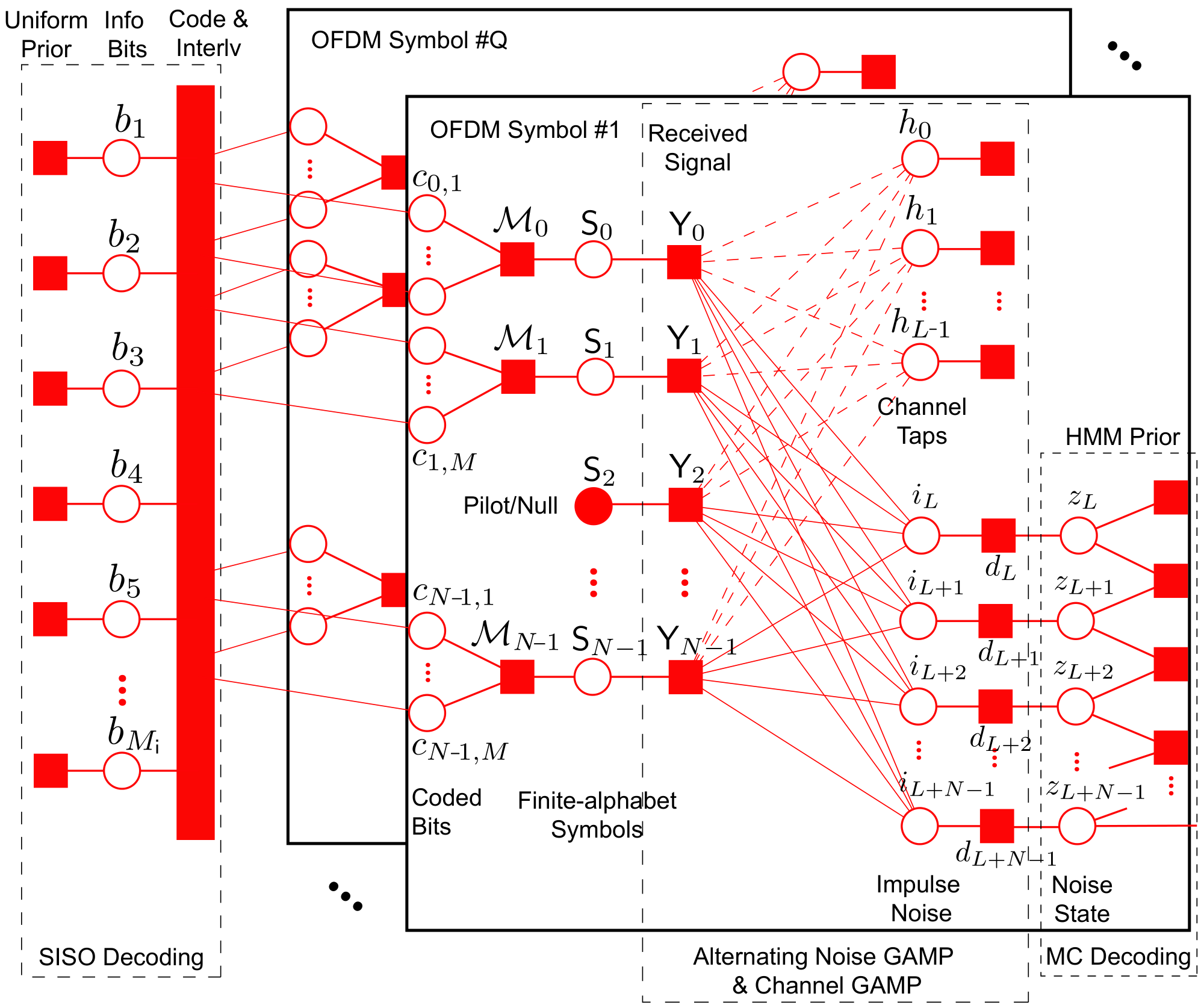
Clearly, direct evaluation of $P(b_{m}|\boldsymbol{\mathsf{Y}})$ from (12) is computationally intractable due to the high-dimensional integrals involved. Belief propagation (BP), and in particular the sum-product algorithm (SPA) [25] described below, offers a practical alternative to direct computation of marginal posteriors. In fact, when the factor graph has no loops, the SPA performs exact inference after only two rounds of message passing (i.e., forward and backward). On the other hand, when the factor graph is loopy, the computation of exact marginal posteriors is generally NP hard [40] and thus the posteriors computed by BP are generally inexact. Nevertheless, loopy BP has been successfully applied to many important problems, such as multi-user detection [41, 42], turbo decoding [43], LDPC decoding [34], compressed sensing [44, 30], and others.

In fact, for certain large densely loopy graphs that arise in the context of compressed sensing, SPA approximations such as the AMP [44] and GAMP [30] algorithms are known to obey a state evolution whose fixed points, when unique, yield exact posteriors [45, 46]. Looking at the factor graph in Fig. 3, we see densely loopy sub-graphs between the factors $\{\mathsf{Y}_{k}\}$ and the time-domain noise samples $\{i_{t}\}$ and channel taps $\{h_{l}\}$, which are due to the linear mixing of the Fourier matrix $\mathbf{F}$. It is these types of densely loopy graphs for which AMP and GAMP are designed.³³ 3 Although rigorous GAMP guarantees have been established only for generalized linear inference problems with i.i.d sub-Gaussian transform matrices [46], equally good performance has been empirically observed over much wider classes of matrices [47]. In the sequel, we will describe exactly how we combine the sum-product and GAMP algorithms for approximate computation of the bit posteriors in (12). First, however, we review the SPA.

Belief propagation (BP) transforms a high-dimensional marginalization problem (like (12)) into a series of local low-dimensional marginalization problems by passing beliefs, or messages, which usually take the form of (possibly un-normalized) pdfs or pmfs, along the edges of a factor graph. The sum-product algorithm (SPA) [25] is probably the best known approach to BP, and it operates according to the following rules:

We now propose a strategy to approximate the bit posteriors in (12) by iterating (an approximation of) the SPA on the loopy factor graph in Fig. 3. To distinguish our approach from others in the literature, we will refer to it as “joint channel, impulse, symbol, and bit estimation” (JCISB).

Given the loopy nature of the factor graph, there exists considerable freedom in the message-passing schedule. In JCISB, we choose to repeatedly pass messages from right to left, and then left to right, as follows.

1. 1.

   Beliefs about coded bits $\{c_{k,m}\}$ flow rightward through the symbol-mapping nodes $\{\mathcal{M}_{k}\}$, the finite-alphabet symbol nodes $\{\mathsf{S}_{k}\}$, and into the factor nodes $\{\mathsf{Y}_{k}\}$.

2. 2.

   GAMP-based messages are then passed repeatedly between the $\{\mathsf{Y}_{k}\}$ and $\{h_{l}\}$ nodes until convergence.

3. 3.

   GAMP-based messages are passed repeatedly between the $\{\mathsf{Y}_{k}\}$ and $\{i_{t}\}$ nodes until convergence, and then through the $\{z_{t}\}$ nodes using the forward-backward algorithm, alternating these two steps until convergence.

4. 4.

   Finally, the messages are propagated from $\{\mathsf{Y}_{k}\}$ leftward through the symbol nodes $\{\mathsf{S}_{k}\}$, the symbol-mapping nodes $\{\mathcal{M}_{k}\}$, the coded-bit nodes $\{c_{k,m}\}$, and the coding-interleaving block—the last step via an off-the-shelf soft-input/soft-output (SISO) decoder.

In the sequel, we will refer to steps 1)–4) as a “turbo” iteration, and to the iterations within step 3) as “impulse iterations,” We note that it is also possible to execute a parallel schedule if the hardware platform supports it. The details of these four message passing steps are given below.

References

- [1] D. Tse and P. Viswanath, Fundamentals of Wireless Communication. Cambridge University Press, 2005.
- [2] K. Blackard, T. Rappaport, and C. Bostian, “Measurements and models of radio frequency impulsive noise for indoor wireless communications,” IEEE J. Sel. Areas Commun., vol. 11, no. 7, pp. 991–1001, 1993.
- [3] W. Lauber and J. Bertrand, “Statistics of motor vehicle ignition noise at VHF/UHF,” IEEE Trans. Electromagn. Compat., vol. 41, no. 3, pp. 257–259, 1999.
- [4] M. Sanchez, L. de Haro, M. Ramon, A. Mansilla, C. Ortega, and D. Oliver, “Impulsive noise measurements and characterization in a UHF digital TV channel,” IEEE Trans. Electromagn. Compat., vol. 41, no. 2, pp. 124–136, 1999.
- [5] M. Sanchez, A. Alejos, and I. Cuinas, “Urban wide-band measurement of the UMTS electromagnetic environment,” IEEE Trans. Veh. Technol., vol. 53, no. 4, pp. 1014–1022, 2004.
- [6] M. Nassar, X. Lin, and B. L. Evans, “Stochastic modeling of microwave oven interference in WLANs,” in IEEE International Conference on Communications, 2011, pp. 1–6.
- [7] M. Nassar, K. Gulati, M. DeYoung, B. L. Evans, and K. Tinsley, “Mitigating near-field interference in laptop embedded wireless transceivers,” Journal of Signal Process. Systems, vol. 63, pp. 1–12, 2011.
- [8] M. Zimmermann and K. Dostert, “Analysis and modeling of impulsive noise in broad-band powerline communications,” IEEE Trans. Electromagn. Compat., vol. 44, no. 1, pp. 249–258, 2002.
- [9] M. Nassar, K. Gulati, Y. Mortazavi, and B. L. Evans, “Statistical modeling of asynchronous impulsive noise in powerline communication networks,” IEEE Global Commun. Conf., pp. 1–6, 2011.
- [10] M. Nassar, J. Lin, Y. Mortazavi, A. Dabak, I. H. Kim, and B. L. Evans, “Local utility power line communications in the 3-500 khz band: Channel impairments, noise, and standards,” IEEE Signal Process. Mag., vol. 29, no. 5, pp. 116–127, 2012.
- [11] S. Zhidkov, “Analysis and comparison of several simple impulsive noise mitigation schemes for OFDM receivers,” IEEE Trans. Commun., vol. 56, no. 1, pp. 5–9, 2008.
- [12] D.-F. Tseng, Y. Han, W. H. Mow, L.-C. Chang, and A. Vinck, “Robust clipping for OFDM transmissions over memoryless impulsive noise channels,” IEEE Commun. Lett., vol. 16, no. 7, pp. 1110–1113, 2012.
- [13] J. Haring, Error Tolerant Communication over the Compound Channel. Shaker-Verlag, 2002.
- [14] J. Haring and A. Vinck, “Iterative decoding of codes over complex numbers for impulsive noise channels,” IEEE Trans. Inf. Theory, vol. 49, no. 5, pp. 1251–1260, 2003.
- [15] A. Mengi and A. Vinck, “Successive impulsive noise suppression in OFDM,” in IEEE International Symposium on Power Line Communications and Its Applications, 2010, pp. 33–37.
- [16] M. Nassar and B. L. Evans, “Low complexity EM-based decoding for OFDM systems with impulsive noise,” in Asilomar Conference on Signals, Systems and Computers, 2011, pp. 1943–1947.
- [17] C.-H. Yih, “Iterative interference cancellation for OFDM signals with blanking nonlinearity in impulsive noise channels,” IEEE Signal Process. Lett., vol. 19, no. 3, pp. 147–150, 2012.
- [18] J. Wolf, “Redundancy, the discrete Fourier transform, and impulse noise cancellation,” IEEE Trans. Commun., vol. 31, no. 3, pp. 458–461, 1983.
- [19] F. Abdelkefi, P. Duhamel, and F. Alberge, “Impulsive noise cancellation in multicarrier transmission,” IEEE Trans. Commun., vol. 53, no. 1, pp. 94–106, 2005.
- [20] ——, “A necessary condition on the location of pilot tones for maximizing the correction capacity in OFDM systems,” IEEE Trans. Commun., vol. 55, no. 2, pp. 356–366, 2007.
- [21] G. Caire, T. Al-Naffouri, and A. Narayanan, “Impulse noise cancellation in OFDM: an application of compressed sensing,” in IEEE International Symposium on Information Theory, 2008, pp. 1293–1297.
- [22] L. Lampe, “Bursty impulse noise detection by compressed sensing,” in IEEE International Symposium on Power Line Communications and Its Applications, 2011, pp. 29–34.
- [23] J. Lin, M. Nassar, and B. L. Evans, “Impulsive noise mitigation in powerline communications using sparse Bayesian learning,” IEEE J. Sel. Areas Commun., vol. 31, no. 7, Jul. 2013.
- [24] A. P. Worthen and W. Stark, “Unified design of iterative receivers using factor graphs,” IEEE Trans. Inf. Theory, vol. 47, no. 2, pp. 843–849, 2001.
- [25] C. Bishop, Pattern Recognition and Machine Learning. Springer, 2006.
- [26] C. Novak, G. Matz, and F. Hlawatsch, “Factor graph based design of an OFDM-IDMA receiver performing joint data detection, channel estimation, and channel length selection,” in ICASSP, 2009, pp. 2561–2564.
- [27] Y. Liu, L. Brunel, and J. Boutros, “Joint channel estimation and decoding using gaussian approximation in a factor graph over multipath channel,” in Proc. IEEE Int. Symp. on Personal, Indoor and Mobile Radio Commun., 2009, pp. 3164–3168.
- [28] G. Kirkelund, C. Manchon, L. Christensen, E. Riegler, and B. Fleury, “Variational message-passing for joint channel estimation and decoding in MIMO-OFDM,” in IEEE Global Telecommun. Conf., 2010, pp. 1–6.
- [29] P. Schniter, “A message-passing receiver for BICM-OFDM over unknown clustered-sparse channels,” IEEE J. Sel. Topics Signal Process., vol. 5, no. 8, pp. 1462–1474, 2011.
- [30] S. Rangan, “Generalized approximate message passing for estimation with random linear mixing,” in IEEE International Symposium on Information Theory (ISIT), 2011, pp. 2174–2178, (See also longer version in Arxiv:1010.5141).
- [31] P. Schniter, “Belief-propagation-based joint channel estimation and decoding for spectrally efficient communication over unknown sparse channels,” Physical Comm., vol. 5, no. 3, pp. 91–101, 2012.
- [32] A. P. Kannu and P. Schniter, “On communication over unknown sparse frequency-selective block-fading channels,” IEEE Trans. Inf. Theory, vol. 56, no. 6, pp. 6619–6632, Oct. 2011.
- [33] P. Schniter, “Turbo reconstruction of structured sparse signals,” in Proc. Conf. on Info. Sciences and Systems, 2010, pp. 1–6.
- [34] D. MacKay, Information Theory, Inference, and Learning Algorithms. Cambridge University Press, 2003.
- [35] P. Schniter and D. Meng, “A message-passing receiver for BICM-OFDM over unknown time-varying sparse channels,” Allerton Conf. Commun. Control Comput., Sep. 2011 (invited).
- [36] D. Middleton, “Non-Gaussian noise models in signal processing for telecommunications: new methods an results for class A and class B noise models,” IEEE Trans. Inf. Theory, vol. 45, no. 4, pp. 1129–1149, 1999.
- [37] J. Ilow and D. Hatzinakos, “Analytic alpha-stable noise modeling in a poisson field of interferers or scatterers,” IEEE Trans. Signal Process., vol. 46, no. 6, pp. 1601–1611, 1998.
- [38] K. Gulati, B. L. Evans, J. Andrews, and K. Tinsley, “Statistics of co-channel interference in a field of poisson and poisson-poisson clustered interferers,” IEEE Trans. Signal Process., vol. 58, no. 12, pp. 6207–6222, 2010.
- [39] S. Fruhwirth-Schnatter, Finite Mixture and Markov Switching Models. Springer, 2006.
- [40] G. F. Cooper, “The computational complexity of probabilistic inference using Bayesian belief networks,” Artificial Intelligence, vol. 42, pp. 393–405, 1990.
- [41] J. Boutros and G. Caire, “Iterative multiuser joint decoding: unified framework and asymptotic analysis,” IEEE Trans. Inf. Theory, vol. 48, no. 7, pp. 1772–1793, 2002.
- [42] D. Guo and C.-C. Wang, “Random sparse linear systems observed via arbitrary channels: A decoupling principle,” in IEEE International Symposium on Information Theory, 2007, pp. 946–950.
- [43] R. McEliece, D. MacKay, and J.-F. Cheng, “Turbo decoding as an instance of Pearl’s “belief propagation” algorithm,” IEEE J. Sel. Areas Commun., vol. 16, no. 2, pp. 140–152, 1998.
- [44] D. Donoho, A. Maleki, and A. Montanari, “Message passing algorithms for compressed sensing,” Proc. Natl. Acad. Sci., vol. 106, pp. 18 914–18 919, 2009.
- [45] M. Bayati and A. Montanari, “The dynamics of message passing on dense graphs, with applications to compressed sensing,” IEEE Trans. Inf. Theory, vol. 57, no. 2, pp. 764–785, 2011.
- [46] A. Javanmard and A. Montanari, “State evolution for general approximate message passing algorithms, with applications to spatial coupling,” arXiv:1211.5164, November 2012.
- [47] H. Monajemi, S. Jafarpour, M. Gavish, Stat 330/CME 362 Collaboration, and D. L. Donoho, “Deterministic matrices matching the compressed sensing phase transitions of Gaussian random matrices,” vol. 110, no. 4, pp. 1181–1186, Jan. 2013.
- [48] R. Negi and J. Cioffi, “Pilot tone selection for channel estimation in a mobile OFDM system,” IEEE Trans. Consum. Eletron., vol. 44, pp. 1122–1128, Aug. 1998.
- [49] Powerline Related Intelligent Metering Evolution (PRIME), Prime Alliance Std. [Online]. Available: http://www.prime-alliance.org
- [50] C. Studer, P. Kuppinger, G. Pope, and H. Bolcskei, “Recovery of sparsely corrupted signals,” IEEE Trans. Inf. Theory, vol. 58, no. 5, pp. 3115–3130, 2012.
- [51] A. Spaulding and D. Middleton, “Optimum reception in an impulsive interference environment–part I: Coherent detection,” IEEE Trans. Commun., vol. 25, no. 9, pp. 910–923, 1977.
- [52] J. P. Vila and P. Schniter, “Expectation-maximization Gaussian-mixture approximate message passing,” arXiv:1207.3107, Jul. 2012.
- [53] I. Kozintsev, “Matlab programs for encoding and decoding of LDPC codes over GF(),” http://www.kozintsev.net/soft.html.
- [54] K. F. Nieman, M. Nassar, J. Lin, and B. L. Evans, “FPGA implementation of a message-passing OFDM receiver for impulsive noise channels,” Asilomar Conf. on Signals, Systems, and Computers, 2013, accepted.
- [55] S. M. Kay, Fundamentals of Statistical Signal Processing: Estimation Theory. Prentice Hall, 1993.