KIC 4544587: an Eccentric, Short Period Binary System with Sct Pulsations and Tidally Excited Modes
Abstract
We present Kepler photometry and ground based spectroscopy of KIC 4544587, a short-period eccentric eclipsing binary system with self-excited pressure and gravity modes, tidally excited modes, tidally influenced p modes, and rapid apsidal motion of 182 y per cycle. The primary and secondary components of KIC 4544587 reside within the Scuti and Dor instability region of the Hurtzsprung-Russell diagram, respectively. By applying the binary modelling software phoebe to prewhitened Kepler photometric data and radial velocity data obtained using the William Herschel Telescope and 4-m Mayall telescope at KPNO, the fundamental parameters of this important system have been determined, including the stellar masses, 1.98 0.07 and 1.60 0.06 , and radii, 1.76 0.03 and 1.42 0.02 , for the primary and secondary components, respectively. Frequency analysis of the residual data revealed 31 modes, 14 in the gravity mode region and 17 in the pressure mode region. Of the 14 gravity modes 8 are orbital harmonics: a signature of tidal resonance. While the measured amplitude of these modes may be partially attributed to residual signal from binary model subtraction, we demonstrate through consideration of the folded light curve that these frequencies do infact correspond to tidally excited pulsations. Furthermore, we present an echelle diagram of the pressure mode frequency region (modulo the orbital frequency) and demonstrate that the tides are also influencing the p modes. A first look at asteroseismology hints that the secondary component is responsible for the p modes, which is contrary to our expectation that the hotter star should pulsate in higher radial overtone, higher frequency p modes.
Keywords:
stars: binaries: eclipsing — stars: binaries: tidal — stars: oscillations – - stars: variable: delta Sct1 Introduction
The Scuti stars form an integral part of the instability strip, spanning a 2-mag range of evolutionary stages, from pre-main sequence to the terminal-age main sequence (Rodríguez & Breger, 2001). Their luminosities range from and their effective temperatures range from K (Buzasi et al., 2005). They oscillate in radial and non-radial pressure modes (p modes) and low order gravity modes (g modes) with observed periods ranging from approximately 18 min to 8 h (Amado et al., 2004; Pamyatnykh, 2000; Grigahcène et al., 2010).

The mechanism is the primary driving mechanism of Scuti pulsations, although Antoci et al. (2011) suggested that one Scuti star may pulsate with stochastically excited modes similar to those seen in the Sun and solar-like pulsators. Delta Scuti stars have a mass range between 1.5 and 2.5 (Lefèvre et al., 2009). At approximately 2 there is a transitional phase where the size of the convective outer envelope becomes negligible for higher mass stars and their outer envelopes become dominated by radiative energy transport; at approximately 1.5 , stars of higher mass develop a convective core (Aerts et al., 2010). As this critical transition in the convective envelope occurs within the range of masses encompassed by Scuti stars, the asteroseismic investigation of Scuti stars may eventually unveil fundamental information pertaining to the physical processes that govern this transition.
Gamma Dor stars are main sequence stars in the temperature range K that pulsate in high order gravity modes driven by convective blocking (Guzik et al., 2000) with pulsation periods typically of the order of 1 d (Grigahcène et al., 2010). As Dor stars are a relatively new class of stars (Balona et al., 1994), until recently their recorded numbers were low and consequently Scuti stars were believed to dominate the classical pulsators on the main sequence (Breger, 2000). However, with the implementation of advanced instruments such as Kepler (Borucki et al., 2010; Gilliland et al., 2010; Batalha et al., 2010), MOST (Walker et al., 2003) and CoRoT (Baglin et al., 2006), many stars demonstrating both Scuti and Dor characteristics have been observed; thus new classification criteria, containing Dor– Scuti and Sct– Dor hybrid stars, have been introduced (Grigahcène et al., 2010). Following this revision, through the characterisation of 750 A-F type main-sequence stars, the percentage of Scuti stars on the main sequence is now estimated to be 27 per cent, Dor stars accounting for 13 per cent, hybrids accounting for 23 per cent and the remaining stars being classified as other types of variables, e.g. spotted stars showing rotational variations (Uytterhoeven et al., 2011).
In a study of 119 A0–A9 stars, 35 5 per cent were found to be in multiple systems (Abt, 2009). However, only 22 per cent of the Scuti stars catalogued are known to be multiple stars (Rodríguez & Breger, 2001). In binary systems the rotational velocity of each stellar component tends towards a velocity that is synchronous with the orbital period as the orbit evolves. As synchronous velocity depends linearly on radius and scales with orbital period (to the power of 2/3), it generally implies an equatorial velocity less than of 120 km s-1 (Abt, 2009), while most Scuti stars are found to have velocities greater than 120 km s-1. Below this value the turbulence in the outer stellar envelope only enables a negligible amount of meridional mixing to occur. This allows for diffusion to take place, which prevents pulsation through the settling of Helium out of the He ii (Breger, 1970). Thus it has previously been assumed that multiplicity indirectly inhibits pulsation. However, there are many cases, including HD 174884 (Maceroni et al., 2009), HD 177863 (Willems & Aerts, 2002), and the newly identified class of eccentric ellipsoidal variables known as Heartbeat stars (Thompson et al., 2012) – including the iconic KOI–54 (Welsh et al., 2011; Fuller & Lai, 2012; Burkart et al., 2012) – that demonstrate how, in some circumstances, multiplicity can not only alter, but increase pulsation amplitudes through the tidal excitation of eigenmodes. It is worthy of note, however, that the existence of tidally driven modes in binary star systems does not invalidate the theory that binarity also indirectly suppresses self-excited modes.
Through the use of binary modelling techniques, direct measurements of stellar masses, radii and distances are possible. Asteroseismic modelling of the identified modes can provide information pertaining to the internal stellar structure and rotation of the pulsating component, making multiple systems with Scuti components extremely valuable. Currently, the thorough asteroseismic analysis of Scuti stars is rarely achieved due to our current inability to model a large number of oscillatory modes excited via the -mechanism. However, with the advent of cutting-edge observations from instruments such as Kepler and CoRoT and new methodologies such as those used by García Hernández et al. (2009) on HD 174936, it is expected that an increasing number of these intriguing objects will be solved in the foreseeable future.
| Identifiers | |
|---|---|
| TYC | 3124-1348-1 |
| GSC | 03124-01348 |
| 2MASS | J19033272+3941003 |
| Position and Brightness | |
| RA (J2000) | 19:03:32.7274 |
| Dec (J2000) | +39:41:00.314 |
| V | 10.8 |
| B | 10.9 |
| Kp | 10.8 |
The Kepler satellite, with its highly precise photometry, is generating observations unparallelled in precision and subsequently giving greater insight into the study of stellar structure through the use of asteroseismology. The primary objective of the Kepler mission is the identification and classification of planets through the transit method. However, the instrumentation required for such observations is highly applicable to the field of asteroseismology (Gilliland et al., 2010). Attributes, such as a stable platform, that enable extended observations, and a precision as good as a few parts per million make the Kepler observations quintessential for the advancement of asteroseismology. A dynamic range of over 10 mag, in addition to a 105 deg2 field of view, give Kepler an unprecedented advantage for obtaining high quality asteroseismic data. Moreover, the ability to generate short cadence data of 1 min time resolution allows for detailed photometric analyses of pulsating stars across the H-R diagram.
KIC 4544587 (where KIC is an acronym for ‘Kepler Input Catalogue’) is an eccentric (), short-period ( d) binary system that contains at least one pulsating component (cf. Table 1 for a list of observable information and identifiers). It was initially identified as a binary by Prša et al. (2011) as part of the first release of the Kepler Eclipsing Binary Catalog (http://keplerebs.villanova.edu). The temperature of the primary component is equivalent to a late A-type star that is within the Scuti instability strip and the secondary component’s temperature is indicative of an early F star, which is likely to be a Dor variable.
Primarily this object was selected as a likely candidate for tidally induced pulsations due to the close proximity of the components at periastron, 4 surface-to-surface. KIC 4544587 also has interesting orbital characteristics including a brightening at periastron in the Kepler photometric light curve due to the combination of tidal distortion and sub-stellar heating. Such a feature is indicative of an eccentric binary with its components in close proximity (Maceroni et al., 2009; Thompson et al., 2012).
In this paper information obtained from modelling the binary features of the photometric and radial velocity curves of KIC 4544587, and the results of the pulsational frequency analysis are presented. In §2 the observations are discussed, including adjustments to the original data set. Sections 3 and 4 describe the spectral disentangling and the atmospheric parameters determined from the disentangled spectra. In §5 the determination of the orbital period is detailed. In §6 the binary light curve modelling method is discussed, which focuses on the use of the binary modelling software, phoebe (Prša & Zwitter, 2005). Section 7 contains the frequency analysis and includes discussion of the evidence for resonance effects. A summary of this paper, with concluding remarks, is given in §8.
2 Observations
2.1 Kepler photometry
| Quarter | Cadence | Number of data points | Duty cycle |
|---|---|---|---|
| 0 | LC | 476 | 99.5% |
| 1 | LC | 1 639 | 98.1% |
| 3.2 | SC | 44 000 | 98.5% |
| 6 | LC | 4 397 | 97.2% |
| 7 | SC | 128 830 | 98.1% |
| 8 | SC | 98 190 | 94.3% |

The Kepler photometric observations of KIC 4544587 consist of both long cadence (hereafter LC) data, during Quarters 0–11, and short cadence (hereafter SC) data during Quarters 3.2, 7, 8, 9 and 10. For our purposes we used a subset of these data up to and including Quarter 8 (see Table 2 and Fig. 1), which were available at the time of analysis. A Quarter is defined as a quarter of a complete, 372.5-d, Kepler orbit around the Sun (Kjeldsen et al., 2010). LC data correspond to a sampling rate of 29.4244 min and SC data to a sampling rate of 58.8488 s. For both formats 6.02-s exposures are co-added on board; this occurs 270 times to form an LC and 9 times to form an SC data point (Caldwell et al., 2010), with any remaining time attributed to readout time. The data are time-stamped with truncated Barycentric Julian date (Gilliland et al., 2010), which is Barycentric Julian date minus 2 400 000. The total Kepler photometric observations that have been analysed span from 2009 May–2011 March and comprise 277 514 data points.
The photometric observations were made using the Kepler broadband filter, which is similar to Cousins . It is advised in the data release notes that accompany the Kepler data that the corrections made in the pipeline can have adverse affects on the binary signal in the data. For this reason the Simple Aperture photometry light curves were used instead of those created by the PPA (Photometer Performance Assessment) portion of the pipeline (Li et al., 2010).
From the total data set, 9471 points were removed as outliers, of which 661 data points were removed from Quarter 3.2, 2 448 from Quarter 7 and 5 597 from Quarter 8. These outliers were selected by eye as the intrinsic variations in the data significantly reduce the effectiveness of automated sigma clipping. Cosmic rays and other noise sources are the dominant causes of outliers and small gaps in the data are also present due to safe mode events, spacecraft rolls and brightening events known as Argabrightening, named after the discoverer, V. Argabright (Van Cleve, 2009). These gaps, however, are minimal, which can be seen by the high duty cycle that was obtained for each Quarter independently, with the exception of the safe mode event at the beginning of Quarter 8.
The SC data have the advantage of increased time resolution, which enables the identification of the p-mode pulsations present in this object (see Fig. 2). Consequently, Quarters 7 and 8 were used for the binary modelling and mode identification of KIC 4544587 (with the exception of modelling the rate of apsidal advance where all LC data were used). A customised target mask was constructed for Quarters 7 and 8 so that the average flux level was consistent over the two quarters. This is important for asteroseismic analysis as quarter-to-quarter flux variations can cause instrumental amplitude modulation in the data. pyKE software (provided by the Kepler Guest Observer office: http://keplergo.arc.nasa.gov/) was used to define the mask, generate the new data files, and convert the data from fits to ascii format. We detrended and normalised each month of data individually by fitting a first or second order Legendre polynomial to segments of data separated by gaps (i.e. caused by spacecraft rolls and safe mode events). As the eclipses affect the detrending process, we elected to fit the polynomials to the out-of-eclipse envelope only. The out-of-eclipse envelope was identified by sigma clipping the data. Using this method we (temporarily) removed all data points 5 above and 0.05 below the light curve. The long-term trends in the out-of-eclipse envelope were then fitted and the trends removed from the original data. Finally, we applied a Fourier transform to the polynomials and found that all significant peaks were d-1, showing that we did not remove any information intrinsic to the system through this method.
As each Kepler pixel is 4 4 arc seconds, it is expected that some contamination may occur within the photometric mask. The contamination value for KIC 4544587, specified by the Kepler Asteroseismic Science Operations Centre (KASOC), is estimated to be 0.019, where 0 implies no contamination and 1 implies complete contamination of the CCD pixels. This contamination value suggests that KIC 4544587 suffers minimally from third light, if at all. We applied the pyKE software to the target pixel files to assess the flux incident on each individual pixel. Light curves for each pixel were generated and the flux distribution over the newly defined masks were examined. From this we determined that the contamination level for KIC 4544587 is negligible.
2.2 Ground-based spectroscopy
| Time | RV1 | RV2 |
|---|---|---|
| (BJD) | km s-1 | km s-1 |
| WHT | ||
| 2455730.62152 | 71.9 5.2 | -133.8 6.5 |
| 2455730.65750 | 91.2 4.7 | -154.5 5.8 |
| 2455730.69932 | 102.2 4.1 | -177.3 5.3 |
| 2455731.55625 | -52.2 5.3 | 30.9 5.7 |
| 2455731.60121 | -62.3 5.3 | 37.8 5.7 |
| 2455731.64668 | -69.4 5.0 | 43.8 5.5 |
| 2455731.70116 | -77.3 4.8 | 50.4 5.9 |
| 2455732.43958 | -79.5 4.9 | 54.9 5.8 |
| 2455732.48500 | -67.9 4.7 | 46.0 5.3 |
| 2455732.52538 | -54.9 4.7 | 36.8 5.9 |
| 2455732.57757 | -38.0 5.0 | 16.1 8.7 |
| 2455732.62238 | -25.4 3.8 | 5.3 9.3 |
| 2455732.65737 | -12.2 4.3 | 19 12 |
| 2455732.69200 | 13.9 9.6 | -52 39 |
| 2455732.72688 | 29.2 3.5 | -103.1 9.2 |
| 2455733.41185 | 46.1 7.3 | -74.6 5.0 |
| 2455733.45956 | -2 22 | -55.3 5.5 |
| 2455733.50435 | -23.6 9.7 | -42.6 5.2 |
| 2455733.54024 | -31.4 5.3 | -22.6 5.9 |
| 2455733.57612 | -32.5 9.7 | -4.6 9.5 |
| 2455733.66781 | -41 17 | 14 14 |
| 2455734.03182 | -73 14 | 51 20 |
| 2455734.43476 | -108.0 7.2 | 79.0 7.4 |
| 2455734.51579 | -100.0 6.8 | 72.8 8.0 |
| 2455734.55967 | -99.2 9.0 | 66.5 8.7 |
| 2455734.60265 | -94.6 9.0 | 53.4 8.9 |
| 2456086.65388 | -108.1 4.2 | 82.3 5.1 |
| 2456087.47573 | 82.3 4.5 | -146.8 5.5 |
| 2456087.57988 | 119.9 4.2 | -193.3 5.3 |
| 2456087.67136 | 123.6 4.2 | -198.0 5.1 |
| 2456087.73410 | 113.4 4.0 | -184.5 5.0 |
| 2456088.61205 | -91.0 4.2 | 59.7 4.9 |
| 2456089.57301 | 37.8 3.8 | -105.8 6.5 |
| 2456089.67823 | 88.0 4.1 | -155.9 4.9 |
| 2456089.73287 | 109.0 4.7 | -181.1 5.6 |
| 2456090.71762 | -79.3 4.4 | 49.7 5.1 |
| 2456091.49676 | -71.9 5.4 | 39.4 6.3 |
| 2456092.44932 | 37 15 | -64.9 7.1 |
| KPNO | ||
| 2456085.68447 | 79.6 2.9 | -138.4 0.8 |
| 2456087.66230 | 127.4 2.9 | -198.0 0.7 |
| 2456087.95906 | 45.6 2.3 | -100.9 1.8 |
| 2456088.70413 | -95.7 3.5 | 75.1 1.9 |
| 2456091.95950 | 126.3 5.0 | -191.4 1.2 |
Thirty eight spectra were obtained using the Intermediate dispersion Spectrograph and Imaging System (ISIS) on the William Herschel Telescope (WHT). The spectra were taken 2011 June 18–21 and 2012 June 7–14 with a resolving power of R 17 000 and 22000, respectively. Calibration exposures using CuAr and CuNe lamps were taken prior to each 300-s exposure of KIC 4544587. Blue and red spectra were obtained using a wavelength coverage of Å and Å respectively. The gratings H2400B (blue arm) and R1200R (red arm) were used. A 0.5-arcsec slit was used to give Nyquist sampling on the CCD and to limit radial velocity errors due to the positioning of the star within the slit. The signal-to-noise obtained was 100 per resolution element. The data were reduced using optimal extraction techniques as implemented in the pamela package (Marsh, 1989).

The initial radial velocity curves were determined using the 2-D cross-correlation technique as implemented in TODCOR (Zucker & Mazeh, 1994) on the red and blue spectra together. The templates for the primary and the secondary component were taken from Castelli & Kurucz (2004) model atmospheres, using T1 = 8250 K, 1 = 4.0, [M/H]1 = 0.0, and T2 = 8000 K, 2 = 4.0, [M/H]2 = 0.0, respectively. Of the 38 spectra taken, cross-correlation failed to produce a good radial velocity fit for 1 spectrum. Subsequent improvement to the radial velocity curves was done by revising the templates according to the best fit photometric model and applying them to both blue and red ends: T1 = 8600 K, 1 = 4.24, and T2 = 7750 K, 2 = 4.33, respectively. A systematic offset slightly larger than 1 was found between the radial velocities of the red arm and the blue arm. As there is no obvious cause for this discrepancy each simultaneous exposure was averaged over the two arms and the discrepancy included in the uncertainty of the radial velocity measurements. The final radial velocity data have a typical 1 uncertainty of 7.3 km s-1 and are listed in Table 3 and depicted in Fig. 3 with the best-fit radial velocity model folded on the period and zero point obtained from the light curve.
Subsequently, five high-resolution spectra were taken using the echelle spectrograph on the 4-m Mayall telescope at KPNO with R 20,000 and a wavelength range of 4500–9000 Å. The data were wavelength-calibrated and flux-normalised as depicted in Fig. 4 where Doppler splitting is clearly visible. As the per-wavelength signal-to-noise ratio of the KPNO spectra is notably lower than the WHT spectra, the 2-D cross-correlation technique, TODCOR, gave significantly larger uncertainties. We consequently used the broadening function technique (Rucinski, 1992) to determine the radial velocities for KPNO spectra. The broadening functions are rotational broadening kernels, where the centroid of the peak yields the Doppler shift and where the width of the peak is a measure of the rotational broadening. For the template we used a radial velocity standard HD 182488, with km/s.

3 Spectral disentangling: orbit
We applied the technique of spectral disentangling (hereafter spd) to isolate spectra for the two binary components individually (Simon & Sturm, 1994). Through this technique we determined the effective temperatures of the two components using the Balmer lines. The medium-resolution ISIS/WHT spectra, described in § 2.2, contain H and H lines, and the medium-resolution echelle KPNO spectra contain H and H lines. The fdbinary11 1 http://sail.zpf.fer.hr/fdbinary code (Ilijic et al., 2004), which is based on a Fourier variant of spd (Hadrava, 1995) was first applied to the time-series of ISIS/WHT spectra since they are more numerous than the KPNO spectra. Since some of the eclipse spectra are affected by the Rossiter-McLaughlin effect, and the line profiles are disturbed, only out-of-eclipse spectra were used. This substantially reduced the number of spectra available for spd, but the phase coverage was still adequate to suppress the undulations in the disentangled spectra of the components (Hensberge et al., 2008). The absence of in-eclipse spectra resulted in an ambiguity in the placement of the continuum of the disentangled spectra. Therefore, we performed spd in separation mode, and then corrected the separated spectra for line-blocking and light dilution using the procedure described in Pavlovski & Hensberge (2005).
In spd individual component spectra are calculated simultaneously and are self-consistently optimised with the orbital parameters, whereby the determination of radial velocities is bypassed (Simon & Sturm, 1994; Hadrava, 1995). In this sense, each individual radial velocity exposure is not optimised and as such no comparison can be made with measured radial velocities (Pavlovski & Hensberge, 2010). The orbital parameters calculated by spd are given in Table 4 and represent the mean values calculated through disentangling 5 short spectral regions from the ISIS/WHT blue spectra, which cover the spectral interval from Å. Telluric lines affect the ISIS/WHT red spectra, which are centred on the H line, thus we removed them manually before the application of spd. Since only five spectra were available in the region of the H line, when using spd, we fixed all the orbital parameters with the exception of the time of periastron.
An important outcome of spd is an enhancement of the S/N ratio in the disentangled spectra, as the spectra are co-added during the spd process. Due to the significant number of WHT/ISIS blue and red spectra, the S/N has vastly improved. However, for the KPNO spectra the gain is small due to limited number of spectra available for analysis. The effect of disentangling on the S/N ratio, for different numbers of input spectra (as well as their original S/N), is clearly depicted in Fig. 5.
| Parameter | SPD |
|---|---|
| Orbital period (d) | 2.189094 (fix) |
| Time of periastron passage, (BJD) | 2455461.450(1) |
| Eccentricity, | 0.288(26) |
| Longitude of periastron, | 328.5(22) |
| Velocity semi-amplitude () | 117.8(9) |
| Velocity semi-amplitude () | 145.8(10) |
| Mass ratio | 0.808(8) |
4 Atmospheric parameters
Once separated, the spectra remain in the common continuum of the binary system, diluted by their companion’s contribution to the total light of the system. The light ratio between the components is derived from the light curve solution and makes renormalisation of the individual component spectra straightforward.We further computed the light ratio for the Johnson (0.685), (0.697) and (0.667) passbands, whilst keeping all other parameters fixed, to determine the deviation of the light ratio as a function of wavelength. We note that the value derived from the light curve using the Kepler passband (0.670) is approximately equal to that of the Johnson band, so we expected that the H line is most affected by our selection as its wavelength is furthest from the Johnson band. Consequently, with the surface gravities of the components known from the complementary light and RV curve solutions, the degeneracy between the effective temperature and the surface gravity can be broken. We determined the components’ effective temperatures by fitting the re-normalised individual spectra with the synthetic theoretical spectra (Tamajo et al., 2011).
The genetic algorithm, as implemented in pikaia (Charbonneau, 1990), was used in the global optimisation of the code starfit (Pavlovski et al., in preparation). A grid of LTE synthetic spectra was calculated using the uclsyn22 2 http://www.astro.keele.ac.uk/bs/publs/uclsyn.pdf code (Smalley et al., 2001) and atlas9 model atmospheres for solar metallcity [M/H] = 0 (Castelli et al., 1997). The grid covers from 6 000 to 10 000 K in steps of 250 K, and g from 3.50 to 4.50 in step of 0.5 dex.
The projected rotational velocities of the components were also optimised. However, as convolution with the rotational kernel has little influence on the broad Balmer lines, we avoided simultaneous determination of the and . Instead, we determined the of the components by fitting the least blended metal lines. The results are given in Table 5. As km s-1, KIC 4544587 has an equitorial velocity of 120 km s-1, below which diffusion can occur. Thus it is likely that the primary component is a metallic-lined Am star (Abt, 2009).

| Parameter | Primary | Secondary |
|---|---|---|
| (K) | 8 090(90) | 7 620(135) |
| (cgs) | 4.22(fixed) | 4.23(fixed) |
| Light factor | 0.670(fixed) | 0.330(fixed) |
| (K) | 8 600(100) | 7 750(180) |
| (cgs) | 4.12(2) | 4.31(2) |
| Light factor | 0.634/0.646/0.670 | 0.366/0.354/0.330 |
| (km s-1) | 86.5(13) | 75.8(15) |
Alongside the optimal fitting of the re-normalised disentangled spectra of H, H, and H lines separately (with the surface gravities and projected rotational velocities held fixed), we have also derived optimal atmospheric parameters in the constrained mode (Tamajo et al., 2011). In constrained mode the light ratio between the components is a free parameter when fitting for the effective temperatures. Also, the surface gravities were left to be free parameters. In the search for the optimal set of parameters, we also adjusted for the velocity shift between disentangled and theoretical spectra, to enable a slight adjustment of the continua of the disentangled spectra. Disentangling the Balmer lines is a difficult task due to their broadening, which is much larger than their Doppler shift. Moreover, when determining the effective temperature, the correct continuum placement is difficult because the Balmer lines of the primary extend over a considerable number of echelle orders, making the correction of the blaze and order merging somewhat uncertain. The optimal set of the parameters obtained when performing constrained fitting, with the light factor as both a free and fixed parameter, is given in Table 5.
5 Period Determination
Period analysis was performed to identify the orbital period of the binary
system. An initial estimate was obtained by applying period04
(Lenz &
Breger, 2004) to the SC data from Quarter 3.2 only. period04
applies a Fourier transform to the data and uses a least-squares fit to optimise
the amplitudes and phases. Further analysis was then performed on all the SC
data (Quarters 3.2, 7 and 8) using kephem (Prša
et al., 2011), an interactive
package with a graphical user interface that incorporates 3 methods: Lomb-
Scargle (LS; Lomb 1976; Scargle 1982), Analysis of
Variance (AoV; Schwarzenberg-Czerny 1989), and
Box-fitting Least Squares (BLS;
Kovács et al. 2002), as implemented in the vartools
package (Hartman et al. 1998). Using kephem, the
period and time of primary minimum were found interactively. The
period was determined by dragging the mouse over a periodogram in the lower
panel of the GUI to see how it affected the alignment of the phased data
presented in the upper panel of the GUI. To determine an accurate period the
zoom tool was utilised on both the periodogram and phased data. The zero point
was then selected by dragging the primary eclipse in the top panel containing
the phased data and align it with zero phase. The ephemeris was found to
be:
MinI = BJD 2455462.006137(9)+2.189094(5) E
where the values in the parentheses give the uncertainty in the previous digits.
The uncertainties were obtained by identifying the range of values that would
yield a visibly indistinguishable result; beyond this uncertainty range the discrepancy is notably increased. Due to apsidal motion the relative separation of the eclipses changes as a function of the rotation of the orbit. Consequently, the period specified is the anomolaus period, which is the period measured by phasing the data on one eclipse (primary eclipse), leaving the other eclipse (secondary eclipse) smeared. Although this is a small effect, the smearing could be seen over the duration of the data used in this analysis. See §6.2 for further discussion on the apsidal motion of KIC 4544587.
6 Binary Modelling
6.1 PHOEBE
phoebe (Prša & Zwitter, 2005) is a binary modelling package based on the Wilson-Devinney (hereafter WD) code (Wilson & Devinney, 1971; Wilson, 1979; Wilson & Van Hamme, 2004). phoebe incorporates all the functionality of the WD code but also provides an intuitive graphical user interface alongside many other improvements that make phoebe highly applicable to the precise Kepler data. These include: uncertainty calculations through heuristical scanning algorithms (which scan parameter space by generating results from multiple starting points to determine the mean and standard deviation); the facility to phase-bin the data; updated filters for the various recent space missions including Kepler; the correct treatment of reddening; and the ability to work with a large number of data points.
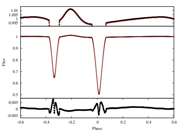
When modelling the data, the initial inputs were a combination of the effective temperatures and values identified through fitting the disentangled spectra with the light factors as a free parameter, 8600 100 K, 7750 180 K, 4.12 and 4.31. We elected to use the results from this mode as a single light factor does not account for the change in each component’s relative light contribution for the different spectral ranges. For the initial investigation a model light curve was generated from the observationally constrained and estimated input parameters. First, the passband luminosity of the model was computed so that the out of eclipse flux levels were correctly positioned with respect to the observed light curve data. Following this the eccentricity () and argument of periastron () were adjusted until the separation between the primary and secondary eclipses, which is proportional to , was equal to that of the observed data. This also involved adjusting the phase shift to retain the position of the model’s eclipses. Once the separation was tightly constrained, the phase shift, and were further adjusted, whilst maintaining the value for , to obtain the relative widths of the primary and secondary eclipses, which are proportional to . The combined depths and widths of the eclipses were then adjusted by altering the inclination and stellar potentials, respectively.
| Parameter | Values |
|---|---|
| Mass ratio | 0.810(12) |
| Primary mass (), | 1.98(7) |
| Secondary mass (), | 1.61(6) |
| Primary radius (), | 1.82(3) |
| Secondary radius (), | 1.58(3) |
| Phase shift | 0.0831(3) |
| Semi-major axis (), | 10.855(46) |
| Orbital eccentricity, | 0.275(4) |
| Argument of periastron (rad), | 5.74(3) |
| Orbital inclination (degrees), | 87.9(3) |
| Primary Teff (K), | 8600(100) |
| Secondary Teff (K), | 7750(180) |
| Primary potential, 1 | 7.09(10) |
| Secondary potential, 2 | 7.12(10) |
| Gamma velocity (km s-1) | -20.13(7) |
| Apsidal Advance (y/cycle) | 182(5) |
| Sidereal Period (d) | 2.1890951(7) |
| Primary relative luminosity | 0.668(2) |
| Secondary relative luminosity | 0.332(1) |
| Primary (cgs), 1 | 4.241(9) |
| Secondary (cgs), 2 | 4.33(1) |
| Primary linear limb darkening coeff. | 0.634 |
| Secondary linear limb darkening coeff. | 0.664 |
| Primary logarithmic limb darkening coeff. | 0.282 |
| Secondary logarithmic limb darkening coeff. | 0.268 |
| Parameter | Values |
| Third light | 0.0 |
| Orbital Period (d) | 2.189094(5) |
| Time of primary minimum (BJD) | 2455462.006137(9) |
| Primary rotation | 1.83 |
| Secondary rotation | 1.83 |
| Primary Bolometric albedo | 1.0 |
| Secondary Bolometric albedo | 1.0 |
| Primary gravity brightening | 1.0 |
| Secondary gravity brightening | 1.0 |
| Primary fine grid raster | 90 |
| Secondary fine grid raster | 90 |
| Primary coarse grid raster | 60 |
| Secondary coarse grid raster | 60 |
Once an initial model had been generated, the differential corrections algorithm was applied in an iterative process to obtain an accurate fit to the light curve data. Once the model was tightly constrained, the radial velocity curves were incorporated to fit the mass ratio, gamma velocity and the projected semi-major axis. As the photometric light curve contains essentially no information about these parameters for a detached system, the fit was performed on the radial velocity curves independently. This avoids improper weighting due to the vastly different number of data points between the different types of curves. Once the best fit solution had been achieved for these parameters the differential corrections algorithm was applied to the light curve for all other parameters specified in Table 6.
When generating the model we assumed pseudo-synchronous stellar rotation after Hut (1981), which was determined to be 1.87 times the orbital period. pseudo-synchronous rotation is indicative of the rotational velocity of the stellar components at periastron. We also fixed the orbital period since kephem is more appropriate for period determination than the differential corrections algorithm. Due to the low contamination and following the analysis of the pixel level data we assumed no third light in the system.


When modelling a binary system with one or more pulsating components (where the pulsations occur on the time scale of the orbit), multiple iterations are required so that the data are thoroughly prewhitened, leaving only the binary signature. This enables the orbital characteristics to be modelled correctly without interference from the stellar pulsations. The method used involved subtracting the computed orbital model from the original observed data, subsequent frequency analysis on the residual data, and finally, the removal of the identified pulsations from the original data. This method is only viable when the pulsations can be considered as perturbations, which is the case for KIC 4544587. What remains is a light curve predominantly free of pulsations for subsequent binary modelling. Three iterations were required when modelling KIC 4544587, with subsequent iterations having negligible effect. The fitted and fixed parameters, and their corresponding values for our best fit model, can be found in Tables 6 and 7 respectively.
The model obtained for KIC 4544587, as seen in Fig. 6, still shows some systematic discrepancies in the residuals during primary and secondary eclipse. These discrepancies arise from a combination of 1) the existence of pulsations that are commensurate with the orbital period and 2) the precise nature of the Kepler data. As some of the pulsations are commensurate with the orbital period, they occur at precisely the same time each orbit. During eclipse phase, however, the relative flux from the pulsating component either increases or decreases, dependent on which star is being eclipsed. This introduces a change in the amplitude of the pulsation during eclipse phase that manifests itself in the residuals of the model. Additionally, the highly precise Kepler data have highlighted the inadequate treatment of parameters such as limb darkening, stellar albedo and the incomplete treatment of surface discretization (Prša et al., 2011), which have previously been considered satisfactory. Currently efforts are being made towards improving the models to account for the physics that has previously been omitted (Prša et al. 2013, in prep.). However, until this major task, which is outside the scope of this paper, is completed, these systematics are unavoidable when generating a binary model of the Kepler data and thus are accounted for in the uncertainties attributed to the fitted parameters.
Uncertainty estimates were obtained using a combination of formal errors, generated by fitting all the parameters simultaneously using phoebe, and those determined through Monte Carlo heuristic scanning. A scan of the parameter space was undertaken for the most correlated parameters using Monte Carlo methods; the results of the Monte Carlo simulations can be found in Figs 7 and 8. The Monte Carlo simulations perturbed the solutions of the best fit model by a predefined amount (5%) in order to identify the spread of possible results and their corresponding 2 values. The 2 values for each solution were then mapped out into confidence intervals which serve as the uncertainty estimates. From the density maps the optimum values of the correlated parameters displayed on the axses can be seen by identifying the combination with the lowest 2 value. The 1 uncertainty values are determined by considering the spread of the innermost contour.

6.2 Orbital Evolution
Apsidal motion is the rotation of the elliptical orbit about the centre of mass (Claret & Gimenez, 1993), which can be caused by the presence of a tertiary component or through the gravitational interactions occurring between the binary components. Using phoebe we determined the rate of apsidal advance for KIC 4544587 to be 0.04306 (2) rad y-1. This equates to a full rotation of the orbit in 182(5) y. Fig. 9 shows the eclipse timing variations of KIC 4544587, and depicts the primary and secondary eclipses moving linearly in opposite directions, which is suggestive of classical apsidal advance caused by tidal disortions. Gies et al. (2012) modelled the eclipse timing variations of 41 eclipsing binaries, including KIC 4544587, and concluded that these variations are a combination of apsidal motion and tidal interactions.
The parameters determined by phoebe are indicative of an eccentric short-period system with two components in close proximity (4.4 surface-to-surface, at periastron). Although the periastron distance is small, we still do not expect any mass transfer as the potentials of the two components far exceed the potential at L1 (4.8), as specified by phoebe.
Eccentric short period binary systems are uncommon due to the rapid rate of circularisation (107 y) compared with the timescale of stellar evolution. Zahn (1975) theorised that orbital circularisation occurs due to the radiative damping of tidally excited oscillations in the stellar outer envelope. For this reason the eccentric short period nature of KIC 4544587 is either the result of tidal capture, recent formation of the system, the presence of a tertiary component or a consequence of its resonant pulsations. As the Kepler field does not contain any prominent star forming regions, it is not expected that KIC 4544587 is a newly formed binary system. Furthermore, as the system is formed from two intermediate mass main sequence stars, it is also unlikely that the system has undergone tidal capture. Thus the eccentric nature of KIC 4544587 is likely a consequence of either a third body or the system’s extreme tidal interactions (see §7.1 for a discussion of tidal resonance).
7 Pulsation Characteristics
| Designation | Frequency | Amplitude | Phase |
|---|---|---|---|
| (d-1) | (flux 10-3) | (rad) | |
| f1 = orb | 0.45681(1) | 1.001 | 0.746(3) |
| f2 = 4orb | 1.82710(1) | 0.593 | 0.3822(4) |
| f3 | 2.01124(1) | 0.561 | 0.0758(5) |
| f4 = 3orb | 1.37041(1) | 0.520 | 0.3514(5) |
| f5 | 3.46822(1) | 0.373 | 0.9864(7) |
| f6 | 48.02231(4) | 0.329 | 0.547(2) |
| f7 = 7orb | 3.19760(2) | 0.244 | 0.301(1) |
| f8 | 41.37020(5) | 0.236 | 0.892(3) |
| f9 | 44.84695(6) | 0.181 | 0.780(3) |
| f10 | 0.12546(3) | 0.164 | 0.996(2) |
| f11 | 46.19662(8) | 0.152 | 0.990(4) |
| f12 | 0.12721(4) | 0.140 | 0.396(2) |
| f13 = 97orb | 44.30982(9) | 0.134 | 0.776(4) |
| f14 = 2orb | 0.91388(4) | 0.133 | 0.026(2) |
| f15 | 48.04449(19) | 0.122 | 0.331(9) |
| f16 = 10orb | 4.56792(4) | 0.116 | 0.532(2) |
| f17 = 8orb | 3.6545(5) | 0.106 | 0.055(2) |
| f18 | 39.54280(11) | 0.106 | 0.984(6) |
| f19 | 1.61186(5) | 0.103 | 0.897(3) |
| f20 | 43.44756(12) | 0.101 | 0.733(6) |
| f21 | 44.81796(12) | 0.099 | 0.088(6) |
| f22 = 9orb | 4.11122(6) | 0.093 | 0.813(3) |
| f23 | 46.58340(13) | 0.092 | 0.056(7) |
| f24 | 0.04089(6) | 0.091 | 0.829(3) |
| f25 | 1.58541(7) | 0.078 | 0.545(3) |
| f26 | 38.22668(16) | 0.076 | 0.109(8) |
| f27 | 44.29902(21) | 0.054 | 0.80(1) |
| f28 | 44.36118(29) | 0.052 | 0.70(1) |
| f29 | 40.05372(23) | 0.051 | 0.30(1) |
| f30 | 46.67401(23) | 0.051 | 0.10(1) |
| f31 | 44.75638(24) | 0.049 | 0.68(1) |
| f32 | 47.95373(26) | 0.045 | 0.69(1) |

The light curve of KIC 4544587 demonstrates clear pulsations in two regions of the frequency spectrum: with periods on the order of days and periods on the order of 30 min, both of which can be seen in the light curve. We used period04 and our own codes to generate a frequency spectrum of the residual data (the detrended data with the orbital fit subtracted), which can be seen in Fig. 10. We also performed eclipse-masking by removing the data points occurring during eclipse phases to remove any residual binary information from the light curve. In the Fourier transform, the gaps created in the data manifest themselves in the window pattern, with peaks separated from the real peak by the orbital frequency. Although this is not ideal, masking is highly important for the identification of resonantly excited modes, which is a crucial aspect of the analysis of KIC 4544587. Without removing the aforementioned points, the systematics would have presented themselves as frequencies at multiples of the orbital frequency, identical to the signature of tidally excited modes, thus masking was required to differentiate between these two possibilities.
period04 incorporates a least squares fitting technique to simultaneously generate amplitudes and phases for all the identified frequencies. For an assumed background level of 40 mag we report the frequencies with amplitudes of 3 or more. The prominent frequency peaks were identified in two regions, d-1 and d-1, which correspond to g modes and p modes, respectively, although the lowest frequency peak (f24 = 0.04089(6) d-1) is possibly due to remaining instrumental effects.
The high frequency, high overtone p-mode frequencies are typical for a Scuti star of temperature similar to that of the primary star, which is towards the hotter, blue edge of the instability strip. An estimate of the radial overtones of the modes can be made from the pulsation constant, , defined by the period-density relation:
| (1) |
which can be rewritten in the form
| (2) |
From the latter relation and the fundamental parameters given in Table 6 we find for the frequency range d-1 for the primary star , and for the secondary star . These are indicative of radial overtones in the range (Stellingwerf, 1979). Pulsation in higher radial overtone p modes such as these (as opposed to pulsation in the fundamental and first overtone modes) is more typical of hotter Sct stars, hence suggests that the p modes arise in the primary star.
We applied a Fourier transform up to the SC Nyquist frequency but did not find any peaks beyond 48.04449(19) d-1. Once the frequencies specified in Table 8 had been prewhitened, an amplitude excess still remained in both the p-mode and g-mode regions. However, as we could not be certain that further detections were real, we did not continue to extract modes beyond this point.
We identified 31 frequencies, 14 in the lower frequency g mode region and 17 p mode region, in the frequency spectrum between 0.1 d-1 and 49 d-1 (see Table 8). Of the 14 g-mode frequencies we identified 8 that are multiples of the orbital frequency (see §7.1).
The remaining g modes are either Dor pulsations, most likely from the secondary component, which is in the Dor instability strip, or non-resonant tidally driven modes, as predicted by Weinberg et al. (2012). Currently we are unable to differentiate as both outcomes have identical signatures, although as the secondary is in the Dor instability strip we would expect it to pulsate with intrinsically excited g modes.
7.1 Tidal Interactions and Combination Frequencies

Tidally excited modes are stellar pulsations that have been excited by the tidal forces of the companion star. A prime example of this is KOI-54 (Welsh et al., 2011). In a binary system with an eccentric orbit, when a stellar eigenfrequency is close to a multiple of the orbital frequency, a near resonance occurs that causes an increase in oscillation amplitude (relative to non-resonant modes). The signature of a tidally excited mode is an oscillation frequency at a multiple of the orbital frequency. We identified 8 frequencies in the g-mode region that are multiples of the orbital frequency. We expect that these are tidally excited l= 2 modes, however, as the eclipses are only partial, we are unable to use the in-eclipse data to determine mode angular degrees or which modes belong to which star. However, as the eclipses are only partial, we are unable to use the in-eclipse data to determine precisely which modes belong to which star.
Previously believed to be short-lived, Witte & Savonije (1999) demonstrated that the duration of tidal resonance can be prolonged through resonant locking. Resonant locking is a result of the change in stellar spin, due to the exchange of angular momentum in the system as the orbit evolves, causing variations in the eigenfrequencies of the stellar components. This, combined with the change in orbital period of the system causes a coupling between the newly resonant eigenfrequency and the orbital frequency, which increases the probability of observing this intriguing phenomenon significantly.
During the identification of the frequencies the data were masked so that the Fourier transform was only applied to the out-of-eclipse data. Consequently, it is unlikely that the presence of these frequencies in the Fourier transform can be completely attributed to an inadequate orbital solution. More convincingly, Fig. 11 shows a magnified image of the out-of-eclipse phase binned data of Quarters 7 and 8 with no frequencies removed (pink, bottom curve), all the identified frequencies except the orbital harmonics removed (blue, middle curve) and all the identified frequencies removed (green, top curve). The pink light curve is visibly thicker than the blue light curve because the non-commensurate pulsations are still present, although have essentially cancelled out. We have no explanation for these variations other than that they are resonantly excited modes. We have also ruled out spots as the cause of the light curve variations as spots are commensurate with the rotational frequency of the star and not the orbital frequency – our rotational velocity measurements are consistent with pseudo-synchronous velocity, thus we would expect peaks in the Fourier transform at multiples of 1.87 times the orbital frequency if the variations were caused by spots.
The p modes were analysed using the unmasked residual data from Quarters 7 and 8. We generated an echelle diagram (Grec et al., 1983), modulo the orbital frequency, of the p- mode frequencies to identify any regular spacings (cf. Fig. 12). We prewhitened all g modes prior to the identification of the p modes to avoid any crosstalk from window pattern. In Fig. 12 the filled circles represent the frequencies in Table 8 and the open circles represent frequencies with amplitudes in the region relative flux units. The latter are not reported in our table as they are below our predefined confidence limit, although here they highlight the vertical groupings which indicate that many of the p mode frequencies are split by the orbital frequency. Our working hypothesis is that the highest amplitude peak in a vertical group is the self-excited p mode and the remaining p modes in that group are the product of non-linear coupling between the self-excited p modes and tidally induced g modes. To our knowledge this effect has not previously been observed and is considered an important tool for identifying g modes in the Sun (Chapellier et al., 2012). In our case, this deduction suggests that one of the stars is pulsating in both p modes and g modes, information that we could not have determined otherwise. An alternative hypothesis, suggested by Weinberg et al. (2013), states that through non-resonant three wave interactions the dynamical tide can excite daughter p-mode and g-mode waves, however, we refrain from discussing the physical nature of these modes at this time33 3 After this manuscript was submitted, we realized that the g modes whose frequencies are not multiples of the orbital harmonics (i.e. , , , and from Table 8) are indicative of non-linear tidal processes. Specifically, rather than having frequencies at orbital harmonics, these g-modes have frequencies that sum to orbital harmonics. Note that , and . These combination frequencies suggest that these modes are excited by parametric three-mode resonance, as detailed in Weinberg et al. 2012 (Papaloizou & Pringle, 1981)However, the non-linear driving mechanisms may be different for the two pairs of modes listed above. In the language of Weinberg et al. 2012, the excitation of and may be due to non-linear driving by the dynamical tide. Essentially, this is the standard three-mode coupling in which a parent mode non-linearly drives pair of daughter modes whose frequencies sum to that of the parent mode, as observed in the KOI-54 system (Fuller & Lai 2012, Burkart et al. 2012). In this case, the parent mode is the dynamical tide at , which is dominated by a nearly resonant g mode. The origin of and likely can not be explained by this mechanism because there is no visible parent mode at . Instead, these modes are likely excited via non-linear driving by the equilibrium tide. In this case, the ”parent” mode is the component of the equilibrium tide that oscillates at 12 times the orbital frequency (which is is dominated by the f mode rather than a g mode). These findings further substantiate our pulsational models which show that we do not expect to see Dor modes in either componet. .
Combination modes created from the same type of mode, however, have been observed in numerous stars including the Scuti stars FG Virginis (Breger et al., 2005) and KIC 11754974 (Murphy, 2012 submitted), and the white dwarf star GD 358 (Winget et al., 1994). Brickhill (1983) determined that the likely cause of combination frequencies is nonlinear interactions related to convective turn-over timescales. Changes in the convective zone during the pulsation cycle cause a change in the amount of flux attenuation. This distorts the stellar shape and causes the pulsations to deviate from pure sinusoids generating combination frequencies in the Fourier transform.

Wu & Goldreich (2001) demonstrated that non-linear interactions could help with mode identification because non-linear mode coupling will only occur between specific modes and different modes generate different amplitude combinations, e.g. = 2 modes generate larger amplitude combination frequencies than = 1 modes. One of the most challenging requirements of modelling Sct stars is mode identification, thus combination frequencies could be key identifiers to obtaining a true asteroseismic model of the multitude of modes presented by this fascinating object.
7.2 Pulsation frequency modulation: the FM effect
Recently Shibahashi & Kurtz (2012) have shown that pulsating stars in binary orbits have frequency multiplets split by the orbital frequency in their amplitude spectra. This is a simple consequence of the light travel time effect causing the pulsation phases to be periodically modulated by the orbital motion as seen by the observer. When the effect is large enough to be measured, radial velocities can be measured directly from the light curve without the need for spectroscopic radial velocities. Shibahashi & Kurtz (2012) demonstrate this by deriving the mass function from photometric data alone for the K-K binary and A star in the complex multiple system KIC 4150611 to better precision than has been possible with spectroscopic radial velocities.
In the case of KIC 4544587 this effect is not measurable, even at the extremely high precision of the Kepler data. Consequently we are not able to complement our spectrally defined radial velocity points with a photometrically defined radial velocity curve. However, we are able to conclude that the FM (frequency modulation) signature is not present in our frequency spectrum and thus does not interfere with our frequency analysis. Shibahashi & Kurtz (2012) characterise the phase modulation with a parameter, , given by
| (3) |
where is the pulsation period, is the orbital period, is the mass of the primary star, and is the mass ratio. For KIC 4544587 the exact value of depends on which star is considered to be pulsating, which is not yet known, but , in either case, since . For a value of this low, Shibahashi & Kurtz (2012) show that, to first order, a frequency triplet split by the orbital frequency is expected for each pulsation frequency, where the amplitude ratio of the side peaks to the central peak is given by
| (4) |
where , and represent the amplitudes of the peaks at , , and , respectively, where is the orbital frequency. In addition, for this low value of the side peaks have essentially the same amplitude.
Table 8 shows that the highest amplitude p mode in KIC 4544587, d-1, has an amplitude of 329 mag. Therefore, we expect the orbital sidelobes generated by the light travel time effect to have amplitudes for this best case of about 7 mag, which is below the limit of detection in our data, but may ultimately be detectable with a more extensive Kepler data set.
7.3 Stellar Evolution and Pulsation Models
To estimate the frequency content expected for stars similar to KIC 4544587, we calculated stellar evolution and pulsation models for single spherically symmetric non-rotating stars using the mass, radius, and effective temperature constraints obtained from binary modelling and spectroscopic analysis. The models use the stellar evolution and pulsation codes described in Guzik et al. (2000), including an updated version of the Iben (1963, 1965) stellar evolution code with OPAL (Iglesias & Rogers, 1996) opacities, Alexander & Ferguson (1994) low-temperature opacities, the Grevesse-Noels (1993) solar mixture, and the Pesnell (1990) linear nonadiabatic stellar pulsation codes. We did not include diffusive helium, element settling or convective overshooting.
We do not know the interior abundances or ages of these stars. However, we attempted to find evolved models of the same initial composition and age that matched the constraints of the two stars in KIC 4544587. The models that were the closest to satisfying these criteria have helium abundance , metallicity and mixing length/pressure scale height 1.90, very near the values calibrated for the Sun for these evolution and pulsation codes, and the Grevesee-Noels solar abundance mixture (see, e.g., Guzik Mussack, 2010). The age of the models is approximately 235 My. The observational constraints, plus the model parameters for two sets of models are given in Table 9.
Fig. 13 shows the evolution tracks for stars of these masses and the observational constraints. The two coeval models miss the observational constraints by a small amount: it is difficult to find a secondary with a small- enough radius, and a primary that is cool enough, for the same age. To gauge the magnitude of the problem, we also searched for single-star best fit models. We found that we could fit the primary parameters exactly using a model with a higher metallicity (0.023), with age 171 My; the higher metallicity allowed a slightly higher mass and produced the desired lower effective temperature. For the secondary, we needed to reduce the metallicity to 0.016 to reduce the radius; the desired radius of 1.43 is reached at the zero-age main sequence.
| Parameters | Observations | Coeval | Single Best-Fit |
|---|---|---|---|
| Models | Models | ||
| Primary | |||
| Mass (M⊙) | 1.98(7) | 1.95 | 1.98 |
| Radius () | 1.76(3) | 1.73 | 1.76 |
| Teff (K) | 8600(100) | 8774 | 8604 |
| Y | 0.27 | 0.28 | |
| Z | 0.017 | 0.023 | |
| Age (My) | 235 | 171 | |
| Secondary | |||
| Mass (M⊙) | 1.60(6) | 1.57 | 1.60 |
| Radius () | 1.43(2) | 1.48 | 1.43 |
| Teff (K) | 7750(180) | 7543 | 7813 |
| Y | 0.27 | 0.27 | |
| Z | 0.017 | 0.016 | |
| Age (My) | 235 | 0 (ZAMS) | |

We calculated the = 0, 1, and 2 nonadiabatic pulsation frequencies for the models in Table 9. For the models with age 235 My, we find that the 1.95- model is predicted to have only one unstable Sct- type frequency for = 0 (7th overtone, 59.4 d-1), = 1, (56.3 d-1) and = 2 (58.9 d-1). The 1.57- model for the secondary is predicted to have unstable Sct-type frequencies in a very wide range, 21 to 90 d-1 for the = 0 (radial) modes (Fundamental through 10th overtones), 21 to 93 d-1 for the = 1, and 22 to 96 d-1 for the = 2 modes. Overall, the p-mode frequency content of KIC 4544587 seems to correspond better to that of the secondary, contrary to the findings of the Q-value equation, but these calculations do not rule out tidal excitation of modes in the primary.
The predicted unstable frequency content for the best-fit non-coeval models in Column 4 of Table 9 is similar, with the primary showing just a few p modes for each degree = 0, 1 and 2 between 46 and 61 d-1, a little higher but overlapping the p-mode frequency range observed in KIC 4544587. For the 1.60-M⊙ secondary, the range of unstable p modes is a little smaller than for the 1.57-M⊙ higher-metallicity model in column 3 of Table 9, and shows eight unstable modes between 22 and 75 d-1 for each degree = 0, 1 and 2.
We also examined the possibility of unstable g-mode frequencies for these models in the observed range of d-1. While we can find many g modes for either = 1 or = 2 in this frequency range, all of the modes are stable. The models have envelope convection zones that are quite shallow, with a temperature at the base of K, near or a little hotter than the region of second helium ionization. At this location, the convective timescale at the convection zone base is shorter than the pulsation period, so Dor g modes are not expected to be pulsationally unstable via the convective blocking mechanism. Verification of this conclusion using a pulsation code with a time-dependent convection treatment would be worthwhile (see, e.g., Grigahcene et al. 2004, Dupret et al. 2005). On the other hand, in either star, g modes consistent with those observed could be tidally or stochastically excited.
While they are useful to guide expectations for intrinsic pulsation frequencies, these single star non-rotating pulsation and evolution models are not adequate for an asteroseismic analysis. Tidal effects and rotation will distort the stars, and so the pulsation modes observed will not correspond to those calculated assuming spherical symmetry. Mode coupling will alter the observed frequencies. The surfaces of these stars are separated by only 4.3 at periastron. It is unlikely, but possible, that mass transfer occurred during an earlier evolution stage. In addition, tidal forces can cause mixing of hydrogen into the stellar core that would slow the evolution compared to that of single stars and alter the internal structure (Liakos et al., 2012).
8 Summary and Conclusions
We have presented the Kepler photometric and ground based spectroscopic model of KIC 4544587, a detached eclipsing binary system with p-mode and g-mode pulsations, apsidal motion, tidally excited modes and combination frequencies. The SC data of Quarters 7 and 8 were used in the binary modelling and pulsation analysis of KIC 4544587 with the exception of modelling the apsidal motion and eclipse timing variations where all available Quarters were used. Radial velocity curves have been incorporated into the binary model, which were generated from 38 spectra obtained using ISIS on the WHT and five spectra using the echelle spectrograph on the 4 m Mayall telescope at KPNO.
The binary model was created using phoebe in an iterative process where the pulsations were identified in the residuals of the orbital fit and subsequently prewhitened to leave only the binary signature for modelling purposes. We were able to obtain a reasonable, but not completely ideal binary model fit. Primarily this is due to the resonant pulsations in KIC 4544587, which have periods commensurate with the orbital period and do not diminish when phasing the data. However, it is also because of the inadequate treatment of certain physical parameters (most prominently gravity brightening, limb darkening and albedo) in the binary modelling process, highlighted by the precise nature of the Kepler data. Addressing this deficiency is a work in progress (Prša et al. 2013, in prep., Degroote et al. 2014, in prep.).
A best fit model was obtained and uncertainty estimates were determined using a combination of formal errors and Monte Carlo simulations, which were used to determine uncertainties for parameters that are highly correlated. The distributions obtained in these simulations demonstrated minimal degeneracy, attesting to the uniqueness of the obtained binary solution. From the binary model fit we determined the fundamental parameters of the stellar components. These include the mass and radius of the primary Scuti component, and , respectively, and the mass and radius of the secondary component, and . We also determined that the system has rapid apsidal motion, y per cycle, which may be partially attributable to the resonant pulsations.
The binary characteristics were subsequently separated from the inherent pulsations and 31 periodicities were identified, 14 in the g-mode region and 17 in the p-mode region. Of the 14 g-mode pulsations, 8 were found to have frequencies that are multiples of the orbital frequency, therefore we conclude that the majority of these are tidally excited pulsations. Seventeen p-mode frequencies were identified in the residuals, many of which demonstrate separations that are multiples of the orbital frequency. Our current hypothesis is that these are combination modes, formed through the non-linear interactions between p modes and g modes. The stellar pulsation models predict many more unstable p modes for the secondary component than the primary, so it is possible that these p modes originate in the secondary component; however, the secondary could also have a few unstable p modes. The pulsation models show that neither star has a convection zone deep enough to produce unstable g modes, at least via the convective blocking mechanism. The g modes, however, could also be tidally driven and originate with either the primary or secondary. Further investigation into the nonlinear mode interactions and tidal excitation of the pulsation modes will require modelling of pulsations in tidally distorted rotating stars, and is beyond the scope of this paper.
9 Acknowledgements
The authors express their sincere thanks to NASA and the Kepler team for allowing them to work with and analyse the Kepler data, making this work possible. The Kepler mission is funded by NASA’s Science Mission Directorate. This work was also supported by the STFC (Science and Technology Funding Council). We would also like to thank the RAS for providing grants which enabled KH’s attendance at conferences and thus enabled the development of collaborations and the successful completion of this work. AP acknowledges support through NASA Kepler PSP grant NNX12AD20G. The research leading to these results has received funding from the European Research Council under the European Community’s Seventh Framework Programme (FP7/2007–2013)/ERC grant agreement n∘227224 (PROSPERITY), as well as from the Research Council of KU Leuven grant agreement GOA/2008/04. We acknowledge the observations taken using the 4-m Mayall telescope at the NOAO, survey number #11A-0022, and the Isaac Newton Group of Telescopes for the use of the William Herschel Telescope (WHT). The WHT is operated on the island of La Palma by the Isaac Newton Group in the Spanish Observatorio del Roque de los Muchachos of the Instituto de Astrofisica de Canarias. The authors would also like to thank Susan Thompson and William Welsh for their comments and suggestions.
References
- Abt (2009) Abt H. A., 2009, AJ, 138, 28
- Aerts et al. (2010) Aerts C., Christensen-Dalsgaard J., Kurtz D., 2010, Astroseismology. Springer
- Alexander & Ferguson (1994) Alexander D. R., Ferguson J. W., 1994, ApJ, 437, 879
- Amado et al. (2004) Amado P. J., Moya A., Suárez J. C., Martín-Ruiz S., Garrido R., Rodríguez E., Catala C., Goupil M. J., 2004, MNRAS, 352, L11
- Antoci et al. (2011) Antoci V., Handler G., Campante T. L., Thygesen A. O., Moya A., Kallinger T., Stello D., Grigahcène A., Kjeldsen H., Bedding T. R., 2011, Nature, 477, 570
- Baglin et al. (2006) Baglin A., Auvergne M., Boisnard L., Lam-Trong T., Barge P., Catala C., Deleuil M., Michel E., Weiss W., 2006, in 36th COSPAR Scientific Assembly Vol. 36 of COSPAR, Plenary Meeting, CoRoT: a high precision photometer for stellar ecolution and exoplanet finding. pp 3749–+
- Balona et al. (1994) Balona L. A., Krisciunas K., Cousins A. W. J., 1994, MNRAS, 270, 905
- Batalha et al. (2010) Batalha N. M., Borucki W. J., Koch D. G., Bryson S. T., Haas M. R., Brown T. M., Caldwell D. A., Hall J. R., Gilliland R. L., Latham D. W., Meibom S., Monet D. G., 2010, ApJ, 713, L109
- Borucki et al. (2010) Borucki W. J., Koch D., Basri G., Batalha N., Brown T., Caldwell D., et al. 2010, Science, 327, 977
- Breger (1970) Breger M., 1970, in Bulletin of the American Astronomical Society Vol. 2 of Bulletin of the American Astronomical Society, Metallic-line A stars and pulsation.. pp 298–+
- Breger (2000) Breger M., 2000, in M. Breger & M. Montgomery ed., Delta Scuti and Related Stars Vol. 210 of Astronomical Society of the Pacific Conference Series, Scuti stars (Review). pp 3–+
- Breger et al. (2005) Breger M., Lenz P., Antoci V., Guggenberger E., Shobbrook R. R., Handler G., Ngwato B., Rodler F., Rodriguez E., López de Coca P., Rolland A., Costa V., 2005, A&A, 435, 955
- Brickhill (1983) Brickhill A. J., 1983, MNRAS, 204, 537
- Burkart et al. (2012) Burkart J., Quataert E., Arras P., Weinberg N. N., 2012, MNRAS, 421, 983
- Buzasi et al. (2005) Buzasi D. L., Bruntt H., Bedding T. R., Retter A., Kjeldsen H., Preston H. L., Mandeville W. J., Suarez J. C., Catanzarite J., Conrow T., Laher R., 2005, ApJ, 619, 1072
- Caldwell et al. (2010) Caldwell D. A., Kolodziejczak J. J., Van Cleve J. E., Jenkins J. M., Gazis P. R., Argabright V. S., et al. 2010, ApJ, 713, L92
- Castelli et al. (1997) Castelli F., Gratton R. G., Kurucz R. L., 1997, A&A, 318, 841
- Castelli & Kurucz (2004) Castelli F., Kurucz R. L., 2004, ArXiv Astrophysics e-prints
- Chapellier et al. (2012) Chapellier E., Mathias P., Weiss W. W., Le Contel D., Debosscher J., 2012, A&A, 540, A117
- Charbonneau (1990) Charbonneau P., 1990, PhD thesis, UNIVERSITE DE MONTREAL (CANADA).
- Claret & Gimenez (1993) Claret A., Gimenez A., 1993, A&A, 277, 487
- Fuller & Lai (2012) Fuller J., Lai D., 2012, MNRAS, 420, 3126
- García Hernández et al. (2009) García Hernández A., Moya A., Michel E., Garrido R., Suárez J. C., Rodríguez E., Amado P. J., Martín-Ruiz S., 2009, A&A, 506, 79
- Gies et al. (2012) Gies D. R., Williams S. J., Matson R. A., Guo Z., Thomas S. M., Orosz J. A., Peters G. J., 2012, AJ, 143, 137
- Gilliland et al. (2010) Gilliland R. L., Brown T. M., Christensen-Dalsgaard J., Kjeldsen H., Aerts C., et al. 2010, PASP, 122, 131
- Grec et al. (1983) Grec G., Fossat E., Pomerantz M. A., 1983, \solphys, 82, 55
- Grevesse & Noels (1993) Grevesse N., Noels A., 1993, in Prantzos N., Vangioni-Flam E., Casse M., eds, Origin and Evolution of the Elements Cosmic abundances of the elements.. pp 15–25
- Grigahcène et al. (2010) Grigahcène A., Antoci V., Balona L., Catanzaro G., Daszyńska-Daszkiewicz J., Guzik J. A., Handler G., Houdek G., Kurtz D. W., Marconi M., Monteiro M. J. P. F. G., Moya A., Ripepi V., Suárez J.-C., 2010, ApJ, 713, L192
- Grigahcène et al. (2010) Grigahcène A., Uytterhoeven K., Antoci V., Balona L., Catanzaro G., Daszyńska-Daszkiewicz J., Guzik J. A., Handler G., Houdek G., Kurtz D. W., Marconi M., Monteiro M. J. P. F. G., Moya A., Ripepi V., Suárez J.-C., 2010, Astronomische Nachrichten, 331, 989
- Guzik et al. (2000) Guzik J. A., Kaye A. B., Bradley P. A., Cox A. N., Neuforge C., 2000, ApJ, 542, L57
- Guzik & Mussack (2010) Guzik J. A., Mussack K., 2010, ApJ, 713, 1108
- Hadrava (1995) Hadrava P., 1995, A&AS, 114, 393
- Hartmann (1998) Hartmann E., 1998, CAGD, 15, 377
- Hensberge et al. (2008) Hensberge H., Ilijić S., Torres K. B. V., 2008, A&A, 482, 1031
- Hut (1981) Hut P., 1981, A&A, 99, 126
- Iben (1963) Iben Jr. I., 1963, ApJ, 138, 452
- Iben (1965) Iben Jr. I., 1965, ApJ, 141, 993
- Iglesias & Rogers (1996) Iglesias C. A., Rogers F. J., 1996, ApJ, 464, 943
- Ilijic et al. (2004) Ilijic S., Hensberge H., Pavlovski K., Freyhammer L. M., 2004, in Hilditch R. W., Hensberge H., Pavlovski K., eds, Spectroscopically and Spatially Resolving the Components of the Close Binary Stars Vol. 318 of Astronomical Society of the Pacific Conference Series, Obtaining normalised component spectra with FDBinary. pp 111–113
- Kjeldsen et al. (2010) Kjeldsen H., Christensen-Dalsgaard J., Handberg R., Brown T. M., Gilliland R. L., Borucki W. J., Koch D., 2010, Astronomische Nachrichten, 331, 966
- Kovács et al. (2002) Kovács G., Zucker S., Mazeh T., 2002, A&A, 391, 369
- Lefèvre et al. (2009) Lefèvre L., Michel E., Aerts C., Kaiser A., Neiner C., Poretti E., Garrido R., Baglin A., Auvergne M., Catala C., Weiss W., Balaguer-Núñez L., Maceroni C., Ribas I., 2009, Communications in Asteroseismology, 158, 189
- Lenz & Breger (2004) Lenz P., Breger M., 2004, in J. Zverko, J. Ziznovsky, S. J. Adelman, & W. W. Weiss ed., The A-Star Puzzle Vol. 224 of IAU Symposium, Period04: A software package to extract multiple frequencies from real data. pp 786–790
- Li et al. (2010) Li J., Allen C., Bryson S. T., Caldwell D. A., Chandrasekaran H., Clarke B. D., Gunter J. P., Jenkins J. M., Klaus T. C., Quintana E. V., Tenenbaum P., Twicken J. D., Wohler B., Wu H., 2010, in Society of Photo-Optical Instrumentation Engineers (SPIE) Conference Series Vol. 7740 of Society of Photo-Optical Instrumentation Engineers (SPIE) Conference Series, Photometer performance assessment in Kepler science data processing
- Liakos et al. (2012) Liakos A., Niarchos P., Soydugan E., Zasche P., 2012, MNRAS, 422, 1250
- Lomb (1976) Lomb N. R., 1976, Ap&SS, 39, 447
- Maceroni et al. (2009) Maceroni C., Montalbán J., Michel E., Harmanec P., Prsa A., Briquet M., Niemczura E., Morel T., Ladjal D., Auvergne M., Baglin A., Baudin F., Catala C., Samadi R., Aerts C., 2009, A&A, 508, 1375
- Marsh (1989) Marsh T. R., 1989, PASP, 101, 1032
- Pamyatnykh (2000) Pamyatnykh A. A., 2000, in M. Breger & M. Montgomery ed., Delta Scuti and Related Stars Vol. 210 of Astronomical Society of the Pacific Conference Series, Pulsational Instability Domain of Scuti Variables. pp 215–+
- Papaloizou & Pringle (1981) Papaloizou J., Pringle J. E., 1981, MNRAS, 196, 371
- Pavlovski & Hensberge (2005) Pavlovski K., Hensberge H., 2005, A&A, 439, 309
- Pavlovski & Hensberge (2010) Pavlovski K., Hensberge H., 2010, in Prša A., Zejda M., eds, Binaries - Key to Comprehension of the Universe Vol. 435 of Astronomical Society of the Pacific Conference Series, Reconstruction and Analysis of Component Spectra of Binary and Multiple Stars. p. 207
- Pesnell (1990) Pesnell W. D., 1990, ApJ, 363, 227
- Prša et al. (2011) Prša A., Batalha N., Slawson R. W., Doyle L. R., Welsh W. F., Orosz J. A., Seager S., Rucker M., Mjaseth K., Engle S. G., Conroy K., Jenkins J., Caldwell D., Koch D., Borucki W., 2011, AJ, 141, 83
- Prša & Zwitter (2005) Prša A., Zwitter T., 2005, ApJ, 628, 426
- Rodríguez & Breger (2001) Rodríguez E., Breger M., 2001, A&A, 366, 178
- Rucinski (1992) Rucinski S. M., 1992, AJ, 104, 1968
- Scargle (1982) Scargle J. D., 1982, ApJ, 263, 835
- Schwarzenberg-Czerny (1989) Schwarzenberg-Czerny A., 1989, MNRAS, 241, 153
- Shibahashi & Kurtz (2012) Shibahashi H., Kurtz D. W., 2012, MNRAS, 422, 738
- Simon & Sturm (1994) Simon K. P., Sturm E., 1994, A&A, 281, 286
- Smalley et al. (2001) Smalley B., Smith K. C., Dowretsky M. M., 2001
- Stellingwerf (1979) Stellingwerf R. F., 1979, ApJ, 227, 935
- Tamajo et al. (2011) Tamajo E., Pavlovski K., Southworth J., 2011, A&A, 526, A76
- Thompson et al. (2012) Thompson S. E., Everett M., Mullally F., Barclay T., Howell S. B., Still M., Rowe J., Christiansen J. L., Kurtz D. W., Hambleton K., Twicken J. D., Ibrahim K. A., Clarke B. D., 2012, ApJ, 753, 86
- Uytterhoeven et al. (2011) Uytterhoeven K., Moya A., Grigahcène A., Guzik J. A., Gutiérrez-Soto J., Smalley B., Handler G., Balona L. A., Niemczura E., Fox Machado L., Benatti S., Chapellier E., Tkachenko A., 2011, A&A, 534, A125
- Van Cleve (2009) Van Cleve J. E., 2009, (Moffet Field CA: NASA Ames Research Center)
- Walker et al. (2003) Walker G., Matthews J., Kuschnig R., Johnson R., Rucinski S., Pazder J., Burley G., Walker A., Skaret K., Zee R., Grocott S., Carroll K., Sinclair P., Sturgeon D., Harron J., 2003, PASP, 115, 1023
- Weinberg et al. (2013) Weinberg N. N., Arras P., Burkart J., 2013, ArXiv e-prints
- Weinberg et al. (2012) Weinberg N. N., Arras P., Quataert E., Burkart J., 2012, ApJ, 751, 136
- Welsh et al. (2011) Welsh W. F., Orosz J. A., Aerts C., Brown T. M., Brugamyer E., Cochran W. D., Gilliland R. L., Guzik J. A., Kurtz D. W., Latham D. W., Marcy G. W., Quinn S. N., Zima W., Allen C., 2011, ApJS, 197, 4
- Willems & Aerts (2002) Willems B., Aerts C., 2002, in C. Aerts, T. R. Bedding, & J. Christensen-Dalsgaard ed., IAU Colloq. 185: Radial and Nonradial Pulsationsn as Probes of Stellar Physics Vol. 259 of Astronomical Society of the Pacific Conference Series, Tidally Induced Oscillations in Close Binaries. pp 76–+
- Wilson (1979) Wilson R. E., 1979, ApJ, 234, 1054
- Wilson & Devinney (1971) Wilson R. E., Devinney E. J., 1971, ApJ, 166, 605
- Wilson & Van Hamme (2004) Wilson R. E., Van Hamme W., 2004, Computing Binary Star Observables (in Reference Manual to the Wilson-Devinney Program)
- Winget et al. (1994) Winget D. E., Nather R. E., Clemens J. C., Provencal J. L., Kleinman S. J., Bradley P. A., Claver C. F., Dixson J. S., Montgomery M. H., Hansen C. J., Hine B. P., Birch P., Candy M., Marar T. M. K., Seetha S., 1994, ApJ, 430, 839
- Witte & Savonije (1999) Witte M. G., Savonije G. J., 1999, A&A, 350, 129
- Wu & Goldreich (2001) Wu Y., Goldreich P., 2001, ApJ, 546, 469
- Zahn (1975) Zahn J.-P., 1975, A&A, 41, 329
- Zucker & Mazeh (1994) Zucker S., Mazeh T., 1994, ApJ, 420, 806