跳到论文正文
W Papers独立论文阅读器 arXiv:1306.1788 论文正文 计算阅读时间 · 0%
引用这篇论文根据当前论文元数据生成,正式投稿前建议核对。


License: arXiv.org perpetual non-exclusive license
arXiv:1306.1788v2 [math.DS] 10 Jun 2016

Orders that yield homeomorphisms on Bratteli diagrams

Sergey Bezuglyi Address: Department of Mathematics, Institute for Low Temperature Physics, Kharkiv 61103, Ukraine Current address: Department of Mathematics, University of Iowa, Iowa City, 52242 IA, USA Email address: bezuglyi@gmail.com and Reem Yassawi Address: Department of Mathematics, Trent University, Peterborough, Canada Email address: ryassawi@trentu.ca
Abstract.

We call an order ω\omega on a Bratteli diagram BB perfect if its Vershik map is a homeomorphism. In this paper we study the set of orders on a diagram and find necessary and sufficient conditions for an order to be perfect, in particular when the order has several extremal paths. This work generalizes previous results, obtained for finite rank Bratteli diagrams. We describe an explicit procedure to create perfect orderings on Bratteli diagrams based on the study of certain relations between the entries of the diagram’s incidence matrices and properties of the associated graphs, with the latter relations characterizing diagrams which support perfect orderings. Also, we apply our theory to give a new combinatorial proof of the fact that the dimension group of a diagram supporting perfect orderings with kk maximal paths has a copy of ℤk−1\mathbb{Z}^{k-1} contained in their infinitesimal subgroup. Under certain conditions, we show that a similar result holds if the diagram supports countably many maximal paths. Our results are illustrated by numerous examples.

Key words and phrases: 
Bratteli diagrams, Vershik maps
1991 Mathematics Subject Classification
Primary 37B10, Secondary 37A20

1. Introduction

A Bratteli diagram BB (Definition 2.1) is an infinite graph which encodes how a space XBX_{B} is to be cut up into arbitrarily small pieces, in order that a dynamics be defined on it, by shifting these pieces. The space XBX_{B} is represented as the set of infinite paths on BB starting at a distinguished vertex, and the dynamics is given by an order ω\omega (Section 2.2) which describes how those pieces are to be shifted, or stacked. The dynamics φω\varphi_{\omega}, called a Vershik map, consists of moving up the stack, and φω\varphi_{\omega} is defined and continuous everywhere except at points which are always at the top of a tower. In this article we are concerned with characterising perfect orders, which are those where φω\varphi_{\omega} extends to a homeomorphism. We recall the following crucial fact that emphasizes the importance of perfect orderings: the class of aperiodic (Definition 2.2) Bratteli diagrams with perfect orderings is in a one-to-one correspondence with the set of aperiodic homeomorphisms of a Cantor set [Med06].

This paper is a natural extension of our previous work [BKY13] that was devoted to the study of perfect orderings on Bratteli diagrams of finite rank. We summarize in Section 3.1 the relevant results from [BKY13], and refer to the article for a more detailed analysis. We restrict our attention to regular Bratteli diagrams (Definition 2.3). For these diagrams, if ω\omega is any order on BB that admits a Vershik map on XBX_{B}, then this map is unique. For any order ω\omega on a regular diagram BB, the sets Xmax​(ω)X_{\max}(\omega) and Xmin​(ω)X_{\min}(\omega) are closed and nowhere dense in the path set XBX_{B}.

Suppose that the Vershik map φω\varphi_{\omega} can be extended to a homeomorphism. Then the order’s extremal edge structure, called its skeleton (Definition 3.9), constrains its languages (Definition 2.5): words in this language must generate paths in certain directed graphs ℋn\mathcal{H}_{n} (Definition 3.19) that are defined by the skeleton. The skeleton also defines the extension of φω\varphi_{\omega} to the set of maximal paths of ω\omega. This extension must satisfy the properties described in Definition 3.13; we call orders which satisfy these properties a correspondence. Conversely, given a Bratteli diagram, skeleton and a correspondence, our main result is that we characterise, in Theorem 4.6, which orders extend to homeomorphisms, using the fact that their language must correspond to valid Eulerian paths in ℋn\mathcal{H}_{n}.

The last section contains a new proof of known results stated in [GPS95] which, in turn, are based on the earlier paper [Put89]: namely that if GG is the dimension group of a simple Bratteli diagram BB, such that BB supports a perfect order with exactly jj maximal paths and jj minimal paths, then the infinitesimal subgroup of GG contains a subgroup isomorphic to ℤj−1\mathbb{Z}^{j-1}. Our combinatorial proof uses extensively the machinery of skeletons and associated graphs that we have developed, as well as our characterization of diagrams that support perfect orderings in Theorem 4.6. We also show that our proof can be extended to a work for a class of Bratteli diagrams that have countably many extremal paths, and believe that an appropriate version of these results holds for dimension groups of aperiodic diagrams. Here we mention recent results of [Han13], where given a dimension group whose infinitesimal subgroup contains ℤk\mathbb{Z}^{k}, concrete (equal row and column sum) Bratteli diagram representations of these dimension groups are found. Some of the examples in [Han13] can be shown to satisfy the conditions of Theorem 4.6. It would be interesting to characterize the dimension groups of diagrams that support perfect orderings.

We end with a few remarks. We find it useful to include a number of examples in the text that will help the reader to understand the concepts and statements. Our examples are mainly of simple diagrams, but the constructs extend to aperiodic diagrams in a similar fashion. The words “order” and “ordering” are mostly used as synonyms, although we often use the former for a specific order, and the latter for an arbitrary order chosen from 𝒪B\mathcal{O}_{B}.

2. Definitions and notation

2.1. Bratteli diagrams

Definition 2.1.

A Bratteli diagram is an infinite graph B=(V,E)B=(V,E) such that the vertex set V=⋃i≥0ViV=\bigcup_{i\geq 0}V_{i} and the edge set E=⋃i≥1EiE=\bigcup_{i\geq 1}E_{i} are partitioned into disjoint subsets ViV_{i} and EiE_{i} such that

(i) V0={v0}V_{0}=\{v_{0}\} is a single point;

(ii) ViV_{i} and EiE_{i} are finite sets;

(iii) there exist a range map rr and a source map ss from EE to VV such that r⁡(Ei)=Vir(E_{i})=V_{i}, s⁡(Ei)=Vi−1s(E_{i})=V_{i-1}, and s−1​(v)≠∅s^{-1}(v)\neq\emptyset, r−1​(v′)≠∅r^{-1}(v^{\prime})\neq\emptyset for all v∈Vv\in V and v′∈V∖V0v^{\prime}\in V\setminus V_{0}.

The pair (Vi,Ei)(V_{i},E_{i}) or just ViV_{i} is called the ii-th level of the diagram BB. A finite or infinite sequence of edges (ei:ei∈Ei)(e_{i}:e_{i}\in E_{i}) such that r⁡(ei)=s⁡(ei+1)r(e_{i})=s(e_{i+1}) is called a finite or infinite path respectively. We write e⁡(v,v′)e(v,v^{\prime}) to denote a finite path e=(e1,…,ek)e=(e_{1},...,e_{k}) such that s⁡(e)=v(=s⁡(e1))s(e)=v(=s(e_{1})) and r⁡(e)=v′(=r⁡(ek))r(e)=v^{\prime}(=r(e_{k})), and let E⁡(v,v′)E(v,v^{\prime}) denote the set of all such paths. For a Bratteli diagram BB, let XBX_{B} denote the set of infinite paths starting at the top vertex v0v_{0}. We endow XBX_{B} with the topology generated by cylinder sets U(ek,…,en):={x∈XB:xi=ei,i=k,…,n}U(e_{k},\ldots,e_{n}):=\{x\in X_{B}:x_{i}=e_{i},\;i=k,\ldots,n\}, where(ek,…,en)(e_{k},\ldots,e_{n}) is a finite path in BB from level kk to level nn. Then XBX_{B} is a 0-dimensional compact metric space with respect to this topology. We assume throughout the paper that XBX_{B} has no isolated points for all considered Bratteli diagrams BB.

Given a Bratteli diagram BB, the nn-th incidence matrix Fn=(fv,w(n)),n≥0,F_{n}=(f^{(n)}_{v,w}),\ n\geq 0, is a |Vn+1|×|Vn||V_{n+1}|\times|V_{n}| matrix whose entries fv,w(n)f^{(n)}_{v,w} are equal to the number of edges between the vertices v∈Vn+1v\in V_{n+1} and w∈Vnw\in V_{n}, i.e.

fv,w(n)=|{e∈En+1:r(e)=v,s(e)=w}|.f^{(n)}_{v,w}=|\{e\in E_{n+1}:r(e)=v,s(e)=w\}|.

Observe that every vertex v∈Vv\in V is connected to v0v_{0} by a finite path and the set E⁡(v0,v)E(v_{0},v) of all such paths is finite. Set hv(n)=|E⁡(v0,v)|h_{v}^{(n)}=|E(v_{0},v)| for v∈Vnv\in V_{n}. Then

hv(n+1)=∑w∈Vnfv,w(n)​hw(n)​orh(n+1)=Fn​h(n)h_{v}^{(n+1)}=\sum_{w\in V_{n}}f_{v,w}^{(n)}h^{(n)}_{w}\ \mbox{or}\ \ h^{(n+1)}=F_{n}h^{(n)}

where h(n)=(hw(n))w∈Vnh^{(n)}=(h_{w}^{(n)})_{w\in V_{n}}.

Next we define some popular families of Bratteli diagrams. We say that BB is simple if for any level nn there is m>nm>n such that E⁡(v,w)≠∅E(v,w)\neq\emptyset for all v∈Vnv\in V_{n} and w∈Vmw\in V_{m}. We say BB is stationary if Fn=F1F_{n}=F_{1} for all n≥2n\geq 2. We say BB has finite rank if for some kk, |Vn|≤k|V_{n}|\leq k for all n≥1n\geq 1. Let BB have finite rank. We say BB has rank dd if dd is the smallest integer such that |Vn|=d|V_{n}|=d infinitely often. We say that BB has strict rank d if |Vn|=d|V_{n}|=d for each n≥1,n\geq 1, and if |r−1​(v)|≥2|r^{-1}(v)|\geq 2 for each v∈V\V0v\in V\backslash V_{0}. If VV has strict rank dd, we will assume that for any nn the vertex set VnV_{n} does not depend on nn and equals the set VV that has exactly dd vertices. In this article we will consider general Bratteli diagrams, which are not necessarily of finite rank.

For a Bratteli diagram BB, the tail (cofinal) equivalence relation ℰ\mathcal{E} on the path space XBX_{B} is defined as x​ℰ​yx\mathcal{E}y if xn=ynx_{n}=y_{n} for all nn sufficiently large, where x=(xn)x=(x_{n}), y=(yn)y=(y_{n}). Let Xp​e​r={x∈XB:|[x]ℰ|<∞}X_{per}=\{x\in X_{B}:|[x]_{\mathcal{E}}|<\infty\}, with [x]ℰ[x]_{\mathcal{E}} denoting the ℰ\mathcal{E} equivalence class of xx. By definition, we have Xp​e​r={x∈XB:∃n>0​ such that ​(|r−1​(r⁡(xi))|=1​∀i≥n)}X_{per}=\{x\in X_{B}:\exists n>0\mbox{ such that }(|r^{-1}(r(x_{i}))|=1\ \forall i\geq n)\}. A Bratteli diagram BB is called aperiodic if Xp​e​r=∅X_{per}=\emptyset, i.e., every ℰ\mathcal{E}-orbit is countably infinite. Throughout the paper, we only consider aperiodic Bratteli diagrams BB. For these diagrams XBX_{B} is a Cantor set and ℰ\mathcal{E} is a Borel equivalence relation on XBX_{B} with uncountably infinitely many equivalence classes.

Let BB be a Bratteli diagram, and n0=0<n1<n2<…n_{0}=0<n_{1}<n_{2}<\ldots be a strictly increasing sequence of integers. The telescoping of BB to (nk)(n_{k}) is the Bratteli diagram B′B^{\prime}, whose kk-level vertex set Vk′=VnkV_{k}^{\prime}=V_{n_{k}} and whose incidence matrices (Fk′)(F_{k}^{\prime}) are defined by

Fk′=Fnk+1−1∘…∘Fnk,F_{k}^{\prime}=F_{n_{k+1}-1}\circ\ldots\circ F_{n_{k}},

where (Fn)(F_{n}) are the incidence matrices for BB. Thus when one telescopes BB one takes a subsequence of levels {nk}\{n_{k}\} and considers the set E⁡(nk,nk+1)E(n_{k},n_{k+1}) of all finite paths between the levels {nk}\{n_{k}\} and {nk+1}\{n_{k+1}\} as edges of the new diagram. In particular, a Bratteli diagram BB has rank dd if and only if there is a telescoping B′B^{\prime} of BB such that B′B^{\prime} has exactly dd vertices at each level.

Next we define a family of aperiodic diagrams that have an incidence matrix structure that is useful for our purposes.

Definition 2.2.

We define the family 𝒜\mathcal{A} of Bratteli diagrams, all of whose incidence matrices are of the form

(2.1) Fn:=(An(1)0…000An(2)…00⋮⋮⋱⋮⋮00…An(k)0Bn(1)Bn(2)…Bn(k)Cn)F_{n}:=\left(\begin{array}[]{ccccc}A_{n}^{(1)}&0&\ldots&0&0\\ 0&A_{n}^{(2)}&\ldots&0&0\\ \vdots&\vdots&\ddots&\vdots&\vdots\\ 0&0&\ldots&A_{n}^{(k)}&0\\ B_{n}^{(1)}&B_{n}^{(2)}&\ldots&B_{n}^{(k)}&C_{n}\\ \end{array}\right)

where for some sequences (d1(n))n,…,(dk(n))n(d_{1}^{(n)})_{n},\ldots,(d_{k}^{(n)})_{n} and (d(n))n,(d^{(n)})_{n},

  1. (1)

    An(i)A_{n}^{(i)} is a di(n+1)×di(n)d_{i}^{(n+1)}\times d_{i}^{(n)} matrix,

  2. (2)

    all matrices An(i)A_{n}^{(i)}, Bn(i)B_{n}^{(i)} and CnC_{n} are strictly positive, and

  3. (3)

    CnC_{n} is a d(n+1)×d(n)d^{(n+1)}\times d^{(n)} matrix.

2.2. Orders on a Bratteli diagram

A Bratteli diagram B=(V,E)B=(V,E) is called ordered if a linear order ‘>>’ is defined on every set r−1​(v)r^{-1}(v), v∈⋃n≥1Vnv\in\bigcup_{n\geq 1}V_{n}. We use ω\omega to denote the corresponding partial order on EE and write (B,ω)(B,\omega) when we consider BB with the ordering ω\omega. Denote by 𝒪B\mathcal{O}_{B} the set of all orderings on BB.

Every ω∈𝒪B\omega\in\mathcal{O}_{B} defines the lexicographic ordering on the set E⁡(k,l)E(k,l) of finite paths between vertices of levels VkV_{k} and VlV_{l}: (ek+1,…,el)>(fk+1,…,fl)(e_{k+1},...,e_{l})>(f_{k+1},...,f_{l}) if and only if there is ii with k+1≤i≤lk+1\leq i\leq l, ej=fje_{j}=f_{j} for i<j≤li<j\leq l and ei>fie_{i}>f_{i}. It follows that, given ω∈𝒪B\omega\in\mathcal{O}_{B}, any two paths from E⁡(v0,v)E(v_{0},v) are comparable with respect to the lexicographic ordering generated by ω\omega. If two infinite paths are tail equivalent, and agree from the vertex vv onwards, then we can compare them by comparing their initial segments in E⁡(v0,v)E(v_{0},v). Thus ω\omega defines a partial order on XBX_{B}, where two infinite paths are comparable if and only if they are tail equivalent. We call a finite or infinite path e=(ei)e=(e_{i}) maximal (minimal) if every eie_{i} is maximal (minimal) amongst the edges from r−1​(r​(ei))r^{-1}(r(e_{i})).

Notice that, for v∈Vi,i≥1v\in V_{i},\ i\geq 1, the minimal and maximal (finite) paths in E⁡(v0,v)E(v_{0},v) are unique. Denote by Xmax​(ω)X_{\max}(\omega) and Xmin​(ω)X_{\min}(\omega) the sets of all maximal and minimal infinite paths in XBX_{B}, respectively. It is not hard to show that Xmax​(ω)X_{\max}(\omega) and Xmin​(ω)X_{\min}(\omega) are non-empty closed subsets of XBX_{B}; in general, Xmax​(ω)X_{\max}(\omega) and Xmin​(ω)X_{\min}(\omega) may have interior points. For a finite rank Bratteli diagram BB, the sets Xmax​(ω)X_{\max}(\omega) and Xmin​(ω)X_{\min}(\omega) are always finite for any ω\omega, and if BB has rank dd, then each of them have at most dd elements ([BKMS10]). An ordered Bratteli diagram (B,ω)(B,\omega) is called properly ordered if the sets Xmax​(ω)X_{\max}(\omega) and Xmin​(ω)X_{\min}(\omega) are singletons. We denote by 𝒪B​(j)\mathcal{O}_{B}(j) the set of all orders on BB which have jj maximal and jj minimal paths. Thus, in our notation, 𝒪B​(1)\mathcal{O}_{B}(1) is the set of proper orders on BB.

Let (B,ω)(B,\omega) be an ordered Bratteli diagram, and suppose that B′=(V′,E′)B^{\prime}=(V^{\prime},E^{\prime}) is the telescoping of BB to levels (nk)(n_{k}). Let v′∈V′v^{\prime}\in V^{\prime} and suppose that the two edges e1′,e_{1}^{\prime}, e2′e_{2}^{\prime}, both with range v′v^{\prime}, correspond to the finite paths e1e_{1}, e2e_{2} in BB, both with range vv. Define the order ω′\omega^{\prime} on B′B^{\prime} by e1′<e2′e_{1}^{\prime}<e_{2}^{\prime} if and only if e1<e2e_{1}<e_{2}. Then ω′\omega^{\prime} is called the lexicographic order generated by ω\omega and is denoted by ω′=L⁡(ω)\omega^{\prime}=L(\omega). It is not hard to see that if ω′=L⁡(ω)\omega^{\prime}=L(\omega), then

|Xmax​(ω)|=|Xmax​(ω′)|,|Xmin​(ω)|=|Xmin​(ω′)|.|X_{\max}(\omega)|=|X_{\max}(\omega^{\prime})|,\ \ |X_{\min}(\omega)|=|X_{\min}(\omega^{\prime})|.

If BB is an aperiodic Bratteli diagram and ω∈𝒪B\omega\in\mathcal{O}_{B}, then Xmax​(ω)∩Xmin​(ω)=∅X_{\max}(\omega)\cap X_{\min}(\omega)=\emptyset.

Definition 2.3.

A Bratteli diagram BB is called regular if for any ordering ω∈𝒪B\omega\in\mathcal{O}_{B} the sets Xmax​(ω)X_{\max}(\omega) and Xmin​(ω)X_{\min}(\omega) have empty interior.

In particular, finite rank Bratteli diagrams are regular, and if all incidence matrix entries of BB are at least 2, then BB is regular. In this article we assume that all diagrams are regular.

Definition 2.4.

Let (B,ω)(B,\omega) be an ordered, regular Bratteli diagram. We say that φ=φω:XB→XB\varphi=\varphi_{\omega}:X_{B}\rightarrow X_{B} is a Vershik map if it satisfies the following conditions:

(i) φ\varphi is a homeomorphism of the Cantor set XBX_{B};

(ii) φ⁡(Xmax​(ω))=Xmin​(ω)\varphi(X_{\max}(\omega))=X_{\min}(\omega);

(iii) if an infinite path x=(x1,x2,…)x=(x_{1},x_{2},\ldots) is not in Xmax​(ω)X_{\max}(\omega), then φ⁡(x1,x2,…)=(x10,…,xk−10,xk¯,xk+1,xk+2,…)\varphi(x_{1},x_{2},\ldots)=(x_{1}^{0},\ldots,x_{k-1}^{0},\overline{x_{k}},x_{k+1},x_{k+2},\ldots), where k=min{n≥1:xn is not maximal}k=\min\{n\geq 1:x_{n}\mbox{ is not maximal}\}, xk¯\overline{x_{k}} is the successor of xkx_{k} in r−1​(r​(xk))r^{-1}(r(x_{k})), and (x10,…,xk−10)(x_{1}^{0},\ldots,x_{k-1}^{0}) is the minimal path in E⁡(v0,s⁡(xk¯))E(v_{0},s(\overline{x_{k}})).

If ω\omega is an ordering on BB, then one can always define the map φ0\varphi_{0} that maps XB∖Xmax​(ω)X_{B}\setminus X_{\max}(\omega) onto XB∖Xmin​(ω)X_{B}\setminus X_{\min}(\omega) according to (iii) of Definition 2.4. The question about the existence of the Vershik map is equivalent to that of an extension of φ0:XB∖Xmax​(ω)→XB∖Xmin​(ω)\varphi_{0}:X_{B}\setminus X_{\max}(\omega)\to X_{B}\setminus X_{\min}(\omega) to a homeomorphism of the entire set XBX_{B}. If ω\omega is a proper ordering, then φω\varphi_{\omega} is a homeomorphism. For a finite rank Bratteli diagram BB, the situation is simpler than for a general Bratteli diagram because the sets Xmax​(ω)X_{\max}(\omega) and Xmin​(ω)X_{\min}(\omega) are finite. Note that Vershik did not assume that his maps where homeomorphisms, as he was working in the measurable context. We say that an ordering ω∈𝒪B\omega\in\mathcal{O}_{B} is perfect if ω\omega admits a Vershik map φω\varphi_{\omega} on XBX_{B}. Denote by 𝒫B\mathcal{P}_{B} the set of all perfect orderings on BB. We observe that for a regular Bratteli diagram with an ordering ω\omega, the Vershik map φω\varphi_{\omega}, if it exists, is defined in a unique way. Also, a necessary condition for ω∈𝒫B\omega\in\mathcal{P}_{B} is that |Xmax​(ω)|=|Xmin​(ω)||X_{\max}(\omega)|=|X_{\min}(\omega)|. Given (B,ω)(B,\omega) with ω∈𝒫B\omega\in\mathcal{P}_{B}, the uniquely defined system (XB,φω)(X_{B},\varphi_{\omega}) is called a Bratteli-Vershik system.

2.3. The languages of an ordered Bratteli diagram

If VV is a finite alphabet, let V+V^{+} denote the set of nonempty words over V.V. We use the notation W′⊆WW^{\prime}\subseteq W to indicate that W′W^{\prime} is a subword of WW. If W1,W2,…,WnW_{1},W_{2},\ldots,W_{n}, are words, then we let ∏i=1nWi\prod_{i=1}^{n}W_{i} refer to their concatenation.

Let ω\omega be an order on a Bratteli diagram BB. Fix a vertex v∈Vnv\in V_{n} and some level m<nm<n, consider the set E⁡(Vm,v)=⋃v′∈VmE⁡(v′,v)E(V_{m},v)=\bigcup_{v^{\prime}\in V_{m}}E(v^{\prime},v) of all finite paths between vertices of level mm and vv. This set can be ordered by ω\omega: E⁡(Vm,v)={e1,…​ep}E(V_{m},v)=\{e_{1},\ldots e_{p}\} where ei<ei+1e_{i}<e_{i+1} for 1≤i≤p−11\leq i\leq p-1. Define the word w⁡(v,m,n):=s⁡(e1)​s​(e2)​…​s​(ep)w(v,m,n):=s(e_{1})s(e_{2})\ldots s(e_{p}) over the alphabet VmV_{m}. If W=v1​…​vr∈Vn+W=v_{1}\ldots v_{r}\in V_{n}^{+}, let w⁡(W,n−1,n):=∏i=1rw⁡(vi,n−1,n).w(W,n-1,n):=\prod_{i=1}^{r}w(v_{i},n-1,n).

Definition 2.5.

The level-nn language ℒ⁡(B,ω,n)\mathcal{L}(B,\omega,n) of (B,ω)(B,\omega) is

ℒ(B,ω,n):={W:W⊂w(v,n,N), for some v∈VN,N>n}.\mathcal{L}(B,\omega,n):=\{W:\,\,W\subset w(v,n,N),\,\,\mbox{ for some }v\in V_{N},N>n\}\,.

If BB has strict rank dd, then each of the level-nn languages can be defined on a common alphabet VV, and in this case we recover our definition of the language ℒ⁡(B,ω)\mathcal{L}(B,\omega) that we introduced in [BKY13]:

ℒ⁡(B,ω):=lim supnℒ⁡(B,ω,n).\mathcal{L}(B,\omega):=\limsup_{n}\mathcal{L}(B,\omega,n)\,.

3. Skeletons on Bratteli diagrams

3.1. Skeletons and associated graphs on finite rank Bratteli diagrams

In this section we review definitions and results from [BKY13] on finite rank diagrams. We do this mainly to set the stage for generalizing these notions to nonfinite rank diagrams, in Section 3.2. Thus our discussion of finite rank ordered diagrams will be concise. For more details on definitions and results, we refer the reader to Section 3 in [BKY13].

Suppose that BB has strict rank dd. If a maximal (minimal) path MM (mm) goes through the same vertex vMv_{M} (vmv_{m}) at each level of BB, we will call this path vertical. The following proposition characterizes when ω\omega is a perfect order on a finite rank Bratteli diagram, and was proved in ([BKY13, Proposition 3.2, Lemma 3.3]) for finite rank diagrams.

Proposition 3.1.

Let (B,ω)(B,\omega) be an ordered Bratteli diagram.

  1. (1)

    Suppose that BB has strict rank dd and that the ω\omega-maximal and ω\omega-minimal paths M1,…,MkM_{1},...,M_{k} and m1,…,mk′m_{1},...,m_{k^{\prime}} are vertical passing through the vertices vM1,…,vMkv_{M_{1}},\ldots,v_{M_{k}} and vm1,…,vmk′v_{m_{1}},\ldots,v_{m_{k^{\prime}}} respectively. Then ω\omega is perfect if and only if

    1. (a)

      k=k′k=k^{\prime},

    2. (b)

      there is a permutation σ\sigma of {1,…​k}\{1,\ldots k\} such that for each i∈{1,…,k}i\in\{1,...,k\}, vMi​vmj∈ℒ⁡(B,ω)v_{M_{i}}v_{m_{j}}\,\in\mathcal{L}(B,\omega) if and only if j=σ⁡(i)j=\sigma(i).

  2. (2)

    Let B′B^{\prime} be a telescoping of BB. Then ω∈𝒫B\omega\in\mathcal{P}_{B} if and only if ω′=L⁡(ω)∈𝒫B′\omega^{\prime}=L(\omega)\in\mathcal{P}_{B^{\prime}}.

We give an example of how one would apply Proposition 3.1. This example also answers negatively the following question, that is related to Statement 2 of Proposition 3.1. Let BB be a Bratteli diagram and B′B^{\prime} a telescoping of BB. Is it true that any perfect order on B′B^{\prime} is obtained by telescoping of a perfect order on BB?

Example 3.2.

We define a stationary Bratteli diagram BB such that for a telescoped diagram B′B^{\prime} there is a perfect order ω′∈𝒫B′\omega^{\prime}\in\mathcal{P}_{B^{\prime}} satisfying the condition ω′≠L⁡(ω)\omega^{\prime}\neq L(\omega) for any perfect order ω\omega on BB.

Let BB be a stationary Bratteli diagram defined on the set of four vertices {a,b,c,d}\{a,b,c,d\} by the incidence matrix

F=(2111121111211112).F=\left(\begin{array}[]{cccc}2&1&1&1\\ 1&2&1&1\\ 1&1&2&1\\ 1&1&1&2\\ \end{array}\right).

Let B′B^{\prime} be the diagram obtained by telescoping BB to all odd levels; it has incidence matrix

F′=F2=(7666676666766667).F^{\prime}=F^{2}=\left(\begin{array}[]{cccc}7&6&6&6\\ 6&7&6&6\\ 6&6&7&6\\ 6&6&6&7\\ \end{array}\right).

In order to define a perfect order ω′\omega^{\prime}, we let, for each nn, w⁡(a,n,n+1)=(a​d​b​c)6​aw(a,n,n+1)=(adbc)^{6}a, w⁡(b,n,n+1)=(b​c​a​d)6​bw(b,n,n+1)=(bcad)^{6}b, w⁡(c,n,n+1)=(c​a​d​b)6​cw(c,n,n+1)=(cadb)^{6}c, and, finally, for r−1​(d)r^{-1}(d) we set w⁡(d,n,n+1)=b​c​a​d7​(b​c​a)5w(d,n,n+1)=bcad^{7}(bca)^{5}. This appearance of d7d^{7} prevents ω′\omega^{\prime} from being a lexicographical order on B′B^{\prime} generated by any choice of ω\omega on BB. On the other hand, using Proposition 3.1, we can verify that ω′∈𝒫B′\omega^{\prime}\in\mathcal{P}_{B^{\prime}}. For, the set of words of length 2 that belong to ℒ⁡(B′,ω′)\mathcal{L}(B^{\prime},\omega^{\prime}) are {a​b,a​d,b​c,c​a,d​b,d​d}\{ab,ad,bc,ca,db,dd\} and σ:{a,b,c}→{a,b,c}\sigma:\{a,b,c\}\rightarrow\{a,b,c\} defined by σ⁡(a)=b,\sigma(a)=b, σ⁡(b)=c\sigma(b)=c and σ⁡(c)=a\sigma(c)=a satisfies part (1) of Proposition 3.1.

Let ω\omega be an order on a Bratteli diagram BB. If v∈V\V0v\in V\backslash V_{0}, we denote the minimal edge with range vv by e¯v\overline{e}_{v} , and we denote the maximal edge with range vv by e~v\widetilde{e}_{v}.

Definition 3.3.

Let (B,ω)(B,\omega) be an ordered rank dd diagram. We say that (B,ω)(B,\omega) is well telescoped if

  1. (1)

    BB has strict rank dd,

  2. (2)

    all ω\omega-extremal paths are vertical, with V~\widetilde{V}, V¯\overline{V} denoting the sets of vertices through which maximal and minimal paths run respectively, and

  3. (3)

    s⁡(e~v)∈V~s(\widetilde{e}_{v})\in\widetilde{V} and s⁡(e¯v)∈V¯s(\overline{e}_{v})\in\overline{V} for each v∈V\(V0∪V1)v\in V\backslash(V_{0}\cup V_{1}), and this is independent of nn.

If (B,ω)(B,\omega) is perfectly ordered, for it to be considered well telescoped, it will also have to satisfy

  1. (4)

    if v~​v¯\widetilde{v}\overline{v} appears as a subword of some w⁡(v,m,n)w(v,m,n) with m≥1m\geq 1, then , then σ⁡(v~)=v¯\sigma(\widetilde{v})=\overline{v} defines a one-to-one correspondence between the sets V~\widetilde{V} and V¯\overline{V}.

Given an ordered finite rank (B,ω)(B,\omega), it can always be telescoped so that it is well telescoped. For details of how this can be done, see Lemma 3.11 in [BKY13]. Thus, when we talk about a (finite rank) ordered diagram, we assume without loss of generality that it is well telescoped. For well telescoped ordered diagrams (B,ω)(B,\omega), we have s⁡(e~v)∈V~ns(\widetilde{e}_{v})\in\widetilde{V}_{n} and s⁡(e¯v)∈V¯ns(\overline{e}_{v})\in\overline{V}_{n} for any v∈Vn+1,n≥1v\in V_{n+1},\ n\geq 1. Given a well telescoped (B,ω)(B,\omega), we call the set ℱω=(V~,V¯,{e~v,e¯v:v∈Vn,n≥2})\mathcal{F}_{\omega}=(\widetilde{V},\overline{V},\{\widetilde{e}_{v},\overline{e}_{v}:v\in V_{n},\,\,n\geq 2\}) the skeleton associated to ω\omega. If ω\omega is a perfect order on BB, it follows that |V¯|=|V~||\overline{V}|=|\widetilde{V}|, and if σ:V~→V¯\sigma:\widetilde{V}\rightarrow\overline{V} is the permutation given by Proposition 3.1, we call σ\sigma the accompanying permutation.

The notion of a skeleton of an ordered diagram can be extended to an unordered diagram. Namely, given a strict rank dd diagram BB, we select, two subsets V~\widetilde{V} and V¯\overline{V} of VV, of the same cardinality, and, for each v∈V\V0∪V1v\in V\backslash V_{0}\cup V_{1}, we select two edges e~v\widetilde{e}_{v} and e¯v\overline{e}_{v}, both with range vv, and such that s⁡(e~v)∈V~s(\widetilde{e}_{v})\in\widetilde{V}, s⁡(e¯v)∈V¯s(\overline{e}_{v})\in\overline{V}. In this way we can extend the definition of a skeleton ℱ=(V~,V¯,{e~v,e¯v:v∈V,})\mathcal{F}=(\widetilde{V},\overline{V},\{\widetilde{e}_{v},\overline{e}_{v}:v\in V,\}) to an unordered strict rank dd Bratteli diagram, with the objective of creating well-telescoped orders. A more detailed discussion can be found in [BKY13]). Arbitrarily choosing a bijection σ:V~→V¯\sigma:\widetilde{V}\rightarrow\overline{V}, we can consider the set of orders on BB which have ℱ\mathcal{F} as skeleton and σ\sigma as accompanying permutation.

Given a skeleton ℱ\mathcal{F} on a finite rank diagram BB, for any vertices v~∈V~\widetilde{v}\in\widetilde{V} and v¯∈V¯\overline{v}\in\overline{V}, we set

(3.1) Wv~={w∈V:s⁡(e~w)=v~}​ and ​Wv¯′={w∈V:s⁡(e¯w)=v¯}.W_{\widetilde{v}}=\{w\in V:s(\widetilde{e}_{w})=\widetilde{v}\}\mbox{ and }W^{\prime}_{\overline{v}}=\{w\in V:s(\overline{e}_{w})=\overline{v}\}.

Then W={Wv~:v~∈V~}W=\{W_{\widetilde{v}}:\widetilde{v}\in\widetilde{V}\} and W′={Wv~′:v¯∈V¯}W^{\prime}=\{W_{\widetilde{v}}^{\prime}:\overline{v}\in\overline{V}\} are both partitions of VV. We call WW and W′W^{\prime} the partitions generated by ℱ\mathcal{F}. Let [v¯,v~]:=Wv¯′∩Wv~[\overline{v},\widetilde{v}]:=W^{\prime}_{\overline{v}}\cap W_{\widetilde{v}}, and define the partition

W∩W′:={[v¯,v~]:v¯∈V¯,v~∈V~,[v¯,v~]≠∅}.W\cap W^{\prime}:=\{[\overline{v},\widetilde{v}]:\overline{v}\in\overline{V},\widetilde{v}\in\widetilde{V},[\overline{v},\widetilde{v}]\neq\emptyset\}.

Let ℱ\mathcal{F} be a skeleton on the strict finite rank BB with accompanying permutation σ\sigma. Let ℋ=(T,P)\mathcal{H}=(T,P) be the directed graph where the set TT of vertices of ℋ\mathcal{H} consists of partition elements [v¯,v~][\overline{v},\widetilde{v}] of W′∩WW^{\prime}\cap W, and where there is an edge in PP from [v¯,v~][\overline{v},\widetilde{v}] to [v¯′,v~′][\overline{v}^{\prime},\widetilde{v}^{\prime}] if and only if v¯′=σ⁡(v~)\overline{v}^{\prime}\,=\sigma(\widetilde{v}). We call ℋ\mathcal{H} the directed graph associated to (B,ℱ,σ)(B,\mathcal{F},\sigma).

Example 3.4.

Suppose that V~=V¯={a,b}\widetilde{V}=\overline{V}=\{a,b\}, σ⁡(a)=a\sigma(a)=a, σ⁡(b)=b\sigma(b)=b, and the set of vertices of ℋ\mathcal{H} is [a,a],[a,b],[b,a],[b,b][a,a],[a,b],[b,a],[b,b]. Then ℋ\mathcal{H} is illustrated in Figure 1. Note that we do not specify a skeleton here. In general, it is possible that for some skeletons one of the vertices [b,a][b,a] or [a,b][a,b] be degenerate, for example, if Wa′∩Wb=∅W_{a}^{\prime}\cap W_{b}=\emptyset, then the vertex [a,b][a,b] is not present in ℋ\mathcal{H}. If the permutation is σ⁡(a)=b\sigma(a)=b, σ⁡(b)=a\sigma(b)=a, then ℋ\mathcal{H} is identical to that of Figure 1, except that the vertices {[a,a],[b,b],[a,b],[b,a]}\{[a,a],\,[b,b],\,[a,b],\,[b,a]\} of the new graph are relabelled {[b,a],[a,b],[b,b],[a,a]}\{[b,a],\,[a,b],\,[b,b],\,[a,a]\} respectively.

Refer to caption

Figure 1. The associated graph ℋ\mathcal{H} for ω∈𝒫B​(2),\omega\in\mathcal{P}_{B}(2), σ⁡(a)=a\sigma(a)=a, σ⁡(b)=b\sigma(b)=b.

Suppose that the strict finite rank BB has skeleton ℱ\mathcal{F} and accompanying permutation σ\sigma. Then any path in ℋ\mathcal{H} corresponds to a family of words in V+V^{+}: for if p1​p2​…​pkp_{1}p_{2}\ldots p_{k} is a path in ℋ\mathcal{H} where pip_{i} has source [v¯i,v~i][\overline{v}_{i},\widetilde{v}_{i}], and for each ii, viv_{i} is any vertex in [v¯i,v~i][\overline{v}_{i},\widetilde{v}_{i}], then the path p1​p2​…​pkp_{1}p_{2}\ldots p_{k} corresponds to the word v1​v2​…​vkv_{1}v_{2}\ldots v_{k} (and many such words can exist). Conversely, if the word v1​v2​…​vkv_{1}v_{2}\ldots v_{k} is such that vi∈[v¯i,v~i]v_{i}\in[\overline{v}_{i},\widetilde{v}_{i}] for each ii, and [v¯1,v~1]​[v¯2,v~2]​…​[v¯k,v~k][\overline{v}_{1},\widetilde{v}_{1}]\,[\overline{v}_{2},\widetilde{v}_{2}]\ldots[\overline{v}_{k},\widetilde{v}_{k}] is a path in ℋ\mathcal{H}, then we say that v1​v2​…​vkv_{1}v_{2}\ldots v_{k} corresponds to a valid path in ℋ\mathcal{H}. The relevance of ℋ\mathcal{H} for perfect orders is described by the following lemma, which was proved in [BKY13, Remark 3.16, Lemma 3.17].

Lemma 3.5.

Let B be a strict finite rank Bratteli diagram, ℱ\mathcal{F} be a skeleton on BB and σ:V~→V¯\sigma:\widetilde{V}\rightarrow\overline{V} be a bijection. Let ℋ\mathcal{H} be the associated directed graph. Suppose that the ordering ω\omega on BB has skeleton and accompanying permutation (ℱ,σ)(\mathcal{F},\sigma), and such that each word in ℒ⁡(B,ω)\mathcal{L}(B,\omega) corresponds to a valid path in ℋ\mathcal{H}. Then ω\omega is perfect. Conversely, if (B,ω)(B,\omega) is a well telescoped, perfectly ordered diagram with skeleton and accompanying permutation (ℱ,σ)(\mathcal{F},\sigma), then every word in ℒ⁡(B,ω)\mathcal{L}(B,\omega) corresponds to a valid path in ℋ\mathcal{H}.

3.2. Skeletons, associated graphs, and correspondences on general Bratteli diagrams

If BB is not of finite rank, the notion of a skeleton can be generalized, although the notation is more technical.

Definition 3.6.

Suppose that (B,ω)(B,\omega) is an ordered Bratteli diagram. To each maximal path MM and minimal path mm we associate the sequences (vn​(M))(v_{n}(M)) and (vn​(m))(v_{n}(m)) of vertices that MM and mm pass through. For each nn, let V~n:={v∈Vn:v=vn​(M)​ for some maximal path ​M}\widetilde{V}_{n}:=\{v\in V_{n}:v=v_{n}(M)\mbox{ for some maximal path }M\}; we call vertices in V~n\widetilde{V}_{n} maximal vertices. Similarly we can define V¯n\overline{V}_{n}, the set of minimal vertices in VnV_{n}.

In other words, for each v~∈V~n\widetilde{v}\in\widetilde{V}_{n}, there is at least one infinite maximal path passing through v~\widetilde{v}, and for each v¯∈V¯n\overline{v}\in\overline{V}_{n}, there is at least one infinite minimal path passing through v¯\overline{v}. The following lemma tells us that the notion of a well telescoped ordered Bratteli diagram can be extended to general Bratteli diagrams:

Proposition 3.7.

Let (B,ω)(B,\omega) be an ordered aperiodic Bratteli diagram. Then there exists a telescoping (B′,ω′)=((V′,E′),ω′)(B^{\prime},\omega^{\prime})=((V^{\prime},E^{\prime}),\omega^{\prime}) of (B,ω)(B,\omega) to a sequence of levels (nk)(n_{k}), such that

  • •

    for every vertex v∈V′v\in V^{\prime}, any maximal edge e~v∈Ek′\widetilde{e}_{v}\in E_{k}^{\prime} has source in V~k−1′\widetilde{V}_{k-1}^{\prime} and any minimal edge e¯v\overline{e}_{v} has source in V¯k−1′\overline{V}_{k-1}^{\prime}, and

  • •

    all of BB’s incidence matrix entries that are nonzero are at least two.

Proof.

We use the idea of the proof of Proposition 2.8 from [HPS92]. Take n1=1n_{1}=1, write V1=V~1∪(V1\V~1)V_{1}=\widetilde{V}_{1}\cup(V_{1}\backslash\widetilde{V}_{1}). Take a vertex v∈V1\V~1v\in V_{1}\backslash\widetilde{V}_{1} and consider all maximal edges ee such that s⁡(e)=vs(e)=v. We say that a maximal edge ee is extendable if there is a maximal edge e′e^{\prime} such that r⁡(e)=s⁡(e′)r(e)=s(e^{\prime}). Let EvE_{v} be the set of all finite maximal paths consisting of extendable edges starting from vv. The set EvE_{v} is finite, and this is true for any v∈V1\V~1v\in V_{1}\backslash\widetilde{V}_{1}. Therefore we can find n2n_{2} such that if ff is a maximal finite path with source in V1\V~1V_{1}\backslash\widetilde{V}_{1}, then r⁡(f)∈Vnr(f)\in V_{n} with n<n2n<n_{2}. Thus, all maximal paths with source in V1V_{1} and range in Vn2V_{n_{2}} must have source in V~1{\widetilde{V}}_{1}. We describe only the next step, the rest following by induction. Write Vn2=V~n2∪(Vn2\V~n2)V_{n_{2}}=\widetilde{V}_{n_{2}}\cup(V_{n_{2}}\backslash\widetilde{V}_{n_{2}}). Find an n3n_{3} such that if ff is a maximal finite path with source in Vn2\V~n2V_{n_{2}}\backslash\widetilde{V}_{n_{2}}, then r⁡(f)∈Vnr(f)\in V_{n} with n<n3n<n_{3}. Therefore all maximal paths with source in Vn2V_{n_{2}} and range in Vn3V_{n_{3}} must have source in V~n2{\widetilde{V}_{n_{2}}}. Continue, and telescope (B,ω)(B,\omega) via levels (nk)(n_{k}). Since maximal edges in Ek′E_{k}^{\prime} in the telescoped diagram (B′,ω′)(B^{\prime},\omega^{\prime}) correspond to maximal paths between Vnk−1V_{n_{k-1}} and VnkV_{n_{k}} in BB, the result follows. An identical argument yields the result for minimal edges. ∎

Definition 3.8.

Let (B,ω)(B,\omega) be an ordered Bratteli diagram, where the sequences (V~n)(\widetilde{V}_{n}) and (V¯n)(\overline{V}_{n}) consist of the maximal and minimal vertices, respectively. Suppose that for each n≥2n\geq 2 and each v∈Vn+1v\in V_{n+1}, s⁡(e~v)∈V~ns(\widetilde{e}_{v})\in\widetilde{V}_{n} and s⁡(e¯v)∈V¯ns(\overline{e}_{v})\in\overline{V}_{n}. Suppose also that all of BB’s nonzero incidence matrix entries are at least two. Then we say that (B,ω)(B,\omega) is well telescoped.

Proposition 3.7 tells us that we can assume that (B,ω)(B,\omega) is well telescoped. Next we generalize the notion of a skeleton to an unordered, non-finite rank Bratteli diagram. Let BB be a Bratteli diagram, where we assume that all nonzero entries of its incidence matrices are at least two.

Definition 3.9.

Let {Mα:α∈I}\{M_{\alpha}:\alpha\in I\}, and {mβ:β∈J},|I|=|J|\{m_{\beta}:\beta\in J\},|I|=|J|, be closed, nowhere dense sets of infinite paths. For n∈ℕn\in\mathbb{N}, let

V~n:={v~:v~=vn​(Mα)​ for some ​α∈I}​ and ​V¯n:={v¯:v¯=vn​(mβ)​ for some ​β∈J}.\widetilde{V}_{n}:=\{\widetilde{v}:\widetilde{v}=v_{n}(M_{\alpha})\mbox{ for some }\alpha\in I\}\mbox{ and }\overline{V}_{n}:=\{\overline{v}:\overline{v}=v_{n}(m_{\beta})\mbox{ for some }\beta\in J\}.

Let {e~v:v∈Vn+1}\{\widetilde{e}_{v}:v\in V_{n+1}\} and {e¯v:v∈Vn+1}\{\overline{e}_{v}:v\in V_{n+1}\} be sets of edges such that r⁡(e~v)=r⁡(e¯v)=vr(\widetilde{e}_{v})=r(\overline{e}_{v})=v, s⁡(e~v)∈V~ns(\widetilde{e}_{v})\in\widetilde{V}_{n} and s⁡(e¯v)∈V¯ns(\overline{e}_{v})\in\overline{V}_{n}. Suppose that for any nn and any N>nN>n,

  1. (1)

    if vN​(Mα)=vN​(Mα′),v_{N}(M_{\alpha})=v_{N}(M_{\alpha}^{\prime}), then vn​(Mα)=vn​(Mα′)v_{n}(M_{\alpha})=v_{n}(M_{\alpha}^{\prime}), with the analogous condition holding for paths mβm_{\beta} and mβ′m_{\beta^{\prime}},

  2. (2)

    if v∈V~n∩V¯nv\in\widetilde{V}_{n}\cap\overline{V}_{n}, then e~v≠e¯v\widetilde{e}_{v}\neq\overline{e}_{v}, and

  3. (3)

    if n∈ℕn\in\mathbb{N}, α∈I\alpha\in I and β∈J\beta\in J, then Mα∈U⁡(e~v)M_{\alpha}\in U(\widetilde{e}_{v}) whenever v=vn​(Mα)v=v_{n}(M_{\alpha}) and mβ∈U⁡(e¯v)m_{\beta}\in U(\overline{e}_{v}) whenever v=vn​(mβ)v=v_{n}(m_{\beta}).

Then we call ℱ=(V~n−1,V¯n−1,{e~v,e¯v:v∈Vn}:n≥2)\mathcal{F}=(\widetilde{V}_{n-1},\overline{V}_{n-1},\{\widetilde{e}_{v},\overline{e}_{v}:v\in V_{n}\}:n\geq 2) the skeleton associated to {Mα:α∈I}\{M_{\alpha}:\alpha\in I\} and {mβ:β∈J}\{m_{\beta}:\beta\in J\}. Vertices in the sets V~n\widetilde{V}_{n} and V¯n\overline{V}_{n} are called maximal and minimal vertices respectively. Paths Mα,α∈I,M_{\alpha},\;\alpha\in I, are called maximal and form the set Xmax​(ℱ)X_{\max}(\mathcal{F}), and paths mβ,β∈J,m_{\beta},\;\beta\in J, are called minimal and form the set Xmin​(ℱ)X_{\min}(\mathcal{F}).

Remark 3.10.

We note the following:

  • •

    If we are given a well telescoped ordered diagram (B,ω)(B,\omega) and |Xmax​(ω)|=|Xmin​(ω)||X_{\max}(\omega)|=|X_{\min}(\omega)|, then we can define the skeleton generated by ω\omega, by letting {Mα:α∈I}=Xmax​(ω)\{M_{\alpha}:\alpha\in I\}=X_{\max}(\omega), {mβ:β∈J}=Xmin​(ω),\{m_{\beta}:\beta\in J\}=X_{\min}(\omega), and choosing for each v∈V\V0∪V1v\in V\backslash V_{0}\cup V_{1}, e~v,e¯v\widetilde{e}_{v},\overline{e}_{v} to be the maximal and minimal edges with range vv respectively. It is clear that if ℱ\mathcal{F} is defined by such an order ω\omega, then Xmax​(ℱ)=Xmax​(ω)X_{\max}(\mathcal{F})=X_{\max}(\omega) and Xmin​(ℱ)=Xmin​(ω)X_{\min}(\mathcal{F})=X_{\min}(\omega).

  • •

    We will not be concerned with orders ω\omega such that |Xmax​(ω)|≠|Xmin​(ω)||X_{\max}(\omega)|\neq|X_{\min}(\omega)|, as our aim is to characterize perfect orders and such a condition would prevent an order from being perfect.

  • •

    The requirement that Xmax​(ℱ)X_{\max}(\mathcal{F}) and Xmin​(ℱ)X_{\min}(\mathcal{F}) be closed is natural: after all, we are introducing skeletons to build orders, and in that case the latter sets must be closed.

  • •

    The regularity of BB leads to the requirement that the sets Xmax​(ω)X_{\max}(\omega) and Xmin​(ω)X_{\min}(\omega) are nowhere dense.

Example 3.11.

Suppose that V0={v0}V_{0}=\{v_{0}\}, and for n≥1n\geq 1, Vn=V~n=V¯n={v1,…​vn}V_{n}=\widetilde{V}_{n}=\overline{V}_{n}=\{v_{1},\ldots v_{n}\}, and all nonzero incidence matrix entries are at least two. Suppose also that for vi∈Vn+1v_{i}\in V_{n+1}, we choose e~i≠e¯i\widetilde{e}_{i}\neq\overline{e}_{i} and define

s(e~vi)={viif i≠n+1 vn if i=n+1, and s(e¯vi)={viif i≠n+1 v1 if i=n+1.s(\widetilde{e}_{v_{i}})=\left\{\begin{array}[]{rl}v_{i}&\mbox{if $i\neq n+1$ }\\ v_{n}&\mbox{ if $i=n+1$}\end{array}\right.,\mbox{ and }\,\,\,s(\overline{e}_{v_{i}})=\left\{\begin{array}[]{rl}v_{i}&\mbox{if $i\neq n+1$ }\\ v_{1}&\mbox{ if $i=n+1$}\end{array}\right.\,.

In Figure 2 we have drawn (only) the extremal edges in BB, with dashed lines represented maximal edges and solid lines representing minimal edges. Consider the sets of infinite paths {Mα:α∈ℕ∪{∞}}\{M_{\alpha}:\alpha\in\mathbb{N}\cup\{\infty\}\} whose edges consist of the identified maximal edges, so that M1M_{1} passes vertically through the vertex v1v_{1} at all levels, and for i>1i>1, MiM_{i} passes through vertices v1v_{1}, v2,…​vi−1,viv_{2},\ldots v_{i-1},v_{i}, and then goes down vertically through viv_{i}. Finally, M∞M_{\infty} passes through vertices v1,v2,v3,…v_{1},v_{2},v_{3},\ldots. Similarly consider the set of infinite paths {mβ:β∈ℕ}\{m_{\beta}:\beta\in\mathbb{N}\} whose edges consist of the identified minimal edges, so that m1m_{1} passes vertically through v1v_{1}, and for i>1i>1, mim_{i} passes through v1v_{1} exactly i−1i-1 times, then jumps to viv_{i} and goes down vertically through viv_{i}. It is straightforward to verify that the sets {Mα:α∈ℕ∪{∞}}\{M_{\alpha}:\alpha\in\mathbb{N}\cup\{\infty\}\} and {mβ:β∈ℕ}\{m_{\beta}:\beta\in\mathbb{N}\} are both countable, closed, and nowhere dense, and that ℱ=(V~n−1,V¯n−1,{e~v,e¯v:v∈Vn}:n≥2)\mathcal{F}=(\widetilde{V}_{n-1},\overline{V}_{n-1},\{\widetilde{e}_{v},\overline{e}_{v}:v\in V_{n}\}:n\geq 2) is the skeleton associated to {Mα:α∈ℕ∪{∞}}\{M_{\alpha}:\alpha\in\mathbb{N}\cup\{\infty\}\} and {mβ:β∈ℕ}\{m_{\beta}:\beta\in\mathbb{N}\}.

Refer to caption

Figure 2. The minimal and maximal edge structure for Example 3.11: solid lines are minimal edges, dashed lines are maximal.
Example 3.12.

Suppose that for n≥1n\geq 1, Vn=V~n=V¯n={v1,…,v2n}V_{n}=\widetilde{V}_{n}=\overline{V}_{n}=\{v_{1},\ldots,v_{2^{n}}\}, and all incidence matrix entries are at least two. We label each vertex vi∈Vnv_{i}\in V_{n} using a binary string (x1,…​xn)(x_{1},\ldots x_{n}) of length nn which denotes i′i^{\prime}s binary expansion, starting with the least significant digit. For example, we label vertex v5∈V4v_{5}\in V_{4} with the string (1010)(1010). Suppose that for vi∈Vn+1v_{i}\in V_{n+1},

s⁡(e~(x1,…,xn+1))=s⁡(e¯(x1,…,xn+1))=(x1,…,xn).s(\widetilde{e}_{(x_{1},\ldots,x_{n+1})})=s(\overline{e}_{(x_{1},\ldots,x_{n+1})})=(x_{1},\ldots,x_{n}).

In this case the sets {Mα:α∈{0,1}ℕ}\{M_{\alpha}:\alpha\in\{0,1\}^{\mathbb{N}}\} and {mα:α∈{0,1}ℕ}\{m_{\alpha}:\alpha\in\{0,1\}^{\mathbb{N}}\} are uncountable.

Note that the previous examples illustrate the fact that when defining a skeleton, we do not need complete information about the Bratteli diagram BB. In particular, at this point, we need to know very little about the incidence matrices (Fn)(F_{n}) of BB. The skeleton ℱ\mathcal{F} is simply a constrained set of choices for all extremal edges when building an order.

Next we discuss a way of building a homeomorphism σ:Xmax​(ℱ)→Xmin​(ℱ)\sigma:X_{\max}(\mathcal{F})\rightarrow X_{\min}(\mathcal{F}) which is amenable to being extended to a Vershik map. This will be the analogue of the permutation associated to a skeleton in the finite rank case.

Suppose that ω\omega is an order on BB. Let σn:V~n→2Vn¯\sigma_{n}:\widetilde{V}_{n}\rightarrow 2^{\overline{V_{n}}} be defined by v¯∈σn​(v~)\overline{v}\in\sigma_{n}(\widetilde{v}) if and only if v~​v¯∈ℒ⁡(B,ω,n)\widetilde{v}\overline{v}\in\mathcal{L}(B,\omega,n). If ω\omega is perfect, then for any sequence (v~n)=(vn​(Mα))(\widetilde{v}_{n})=(v_{n}(M_{\alpha})), there is a unique sequence (v¯n)=(vn​(mβ))(\overline{v}_{n})=(v_{n}(m_{\beta})) with v¯n∈σn​(v~n)\overline{v}_{n}\in\sigma_{n}(\widetilde{v}_{n}) for each nn. If a perfect order ω\omega has a finite number of extremal paths, we can say more. In that case, for all large enough nn, and all maximal v~∈V~n\widetilde{v}\in\widetilde{V}_{n}, σn​(v~)\sigma_{n}(\widetilde{v}) is an element, not a subset, of V¯n\overline{V}_{n} - i.e. each maximal vertex can only be followed by a unique minimal vertex in ℒ⁡(B,ω,n)\mathcal{L}(B,\omega,n). One can then say that for all large nn, |V~n|=|V¯n||\widetilde{V}_{n}|=|\overline{V}_{n}| and σn:V~n→V¯n\sigma_{n}:\widetilde{V}_{n}\rightarrow\overline{V}_{n} is a bijection. In the case of finite rank, the sets V~n\widetilde{V}_{n} and V¯n\overline{V}_{n}, and the maps σn:V~n→V¯n\sigma_{n}:\widetilde{V}_{n}\rightarrow\overline{V}_{n} could be taken to be equal for all nn, and in that case we called σ:=(σn)\sigma:=(\sigma_{n}) a permutation in [BKY13].

In the general case of a perfect order with infinitely many extremal paths, though, this fact - that for any sequence (v~n)=(vn​(Mα))(\widetilde{v}_{n})=(v_{n}(M_{\alpha})), there is a unique sequence (v¯n)=(vn​(mβ))(\overline{v}_{n})=(v_{n}(m_{\beta})) with v¯n∈σn​(v~n)\overline{v}_{n}\in\sigma_{n}(\widetilde{v}_{n}) for each nn - does not generally imply that (v~n)=(vn​(Mα))(\widetilde{v}_{n})=(v_{n}(M_{\alpha})) is eventually a sequence of singletons. The main obstacle is that one can have pairs of distinct maximal paths that agree on an arbitrarily large initial segment. For, suppose that φω​(M)=m\varphi_{\omega}(M)=m, and assume that M′M^{\prime} is another maximal path that coincides with MM for the first nn segments till the vertex v~n\widetilde{v}_{n}. By continuity of φω\varphi_{\omega}, the minimal path m′=φω​(M′)m^{\prime}=\varphi_{\omega}(M^{\prime}) must be close to mm, but it can be that v¯n=vn​(m)≠vn​(m′)=w¯n\overline{v}_{n}=v_{n}(m)\neq v_{n}(m^{\prime})=\overline{w}_{n}. So, we see that not only v~n​v¯n∈L⁡(B,ω,n)\widetilde{v}_{n}\overline{v}_{n}\in L(B,\omega,n) but also v~n​w¯n∈L⁡(B,ω,n)\widetilde{v}_{n}\overline{w}_{n}\in L(B,\omega,n), that is {v¯n,w¯n}∈σn​(v~n)\{\overline{v}_{n},\overline{w}_{n}\}\in\sigma_{n}(\widetilde{v}_{n}). One can build such orders on any Bratteli diagram: see Example 3.

We use these observations to make the following definition, which generalizes the concept of a permutation for finite rank diagrams. Some notation: if σ:V~→2V¯\sigma:\widetilde{V}\rightarrow 2^{\overline{V}} and v¯∈V¯\overline{v}\in\overline{V}, we define σ−1​(v¯):={v~:v¯∈σ⁡(v~)}.\sigma^{-1}(\overline{v}):=\{\widetilde{v}:\overline{v}\in\sigma(\widetilde{v})\}.

Definition 3.13.

Let ℱ\mathcal{F} be a skeleton for an unordered Bratteli diagram BB. Suppose that σ=(σn)n\sigma=(\sigma_{n})_{n} is a sequence of maps σn:V~n→2V¯n\sigma_{n}:\widetilde{V}_{n}\rightarrow 2^{\overline{V}_{n}}, such that for each nn, ⋃v~∈V~nσn​(v~)=V¯n\bigcup_{\widetilde{v}\in\widetilde{V}_{n}}\sigma_{n}(\widetilde{v})=\overline{V}_{n}, and

  1. (1)

    σ\sigma is composition consistent: let M⁡(n,N,v~)M(n,N,\widetilde{v}) and m⁡(n,N,v¯)m(n,N,\overline{v}) denote the maximal and minimal paths from level nn to level N>nN>n with range v~\widetilde{v} and v¯\overline{v} respectively. If v¯∈σN​(v~)\overline{v}\in\sigma_{N}(\widetilde{v}), then s⁡(m⁡(n,N,v¯))∈σn​(s⁡(M⁡(n,N,v~)))s(m(n,N,\overline{v}))\in\sigma_{n}(s(M(n,N,\widetilde{v}))),

  2. (2)

    for any M∈Xmax​(ℱ)M\in X_{\max}(\mathcal{F}), there is a unique m∈Xmin​(ℱ)m\in X_{\min}(\mathcal{F}) with (vn​(m))n∈∏nσn​(vn​(M))(v_{n}(m))_{n}\in\prod_{n}\sigma_{n}(v_{n}(M)),

  3. (3)

    for any m∈Xmin​(ℱ)m\in X_{\min}(\mathcal{F}), there is a unique M∈Xmax​(ℱ)M\in X_{\max}(\mathcal{F}) with (vn​(M))n∈∏nσn−1​(vn​(m))(v_{n}(M))_{n}\in\prod_{n}\sigma_{n}^{-1}(v_{n}(m)), and

  4. (4)

    the bijection σ:Xmax​(ℱ)→Xmin​(ℱ)\sigma:X_{\max}(\mathcal{F})\rightarrow X_{\min}(\mathcal{F}) defined using properties 2 and 3 is a homeomorphism.

Then we say that σ=(σn)\sigma=(\sigma_{n}) is a correspondence associated to ℱ\mathcal{F}.

Example 3.14.

We continue with the skeleton defined in Example 3.11 and Figure 2. Let σ\sigma be defined by

σn​(vi)={{vi+1}if 1≤i≤n−1{v1} if i=n\sigma_{n}(v_{i})=\left\{\begin{array}[]{rl}\{v_{i+1}\}&\mbox{if $1\leq i\leq n-1$}\\ \{v_{1}\}&\mbox{ if $i=n$}\end{array}\right.\,

for each n≥1n\geq 1; then one can verify that σ\sigma is composition consistent. Since each σn:V~n→V¯n\sigma_{n}:\widetilde{V}_{n}\rightarrow\overline{V}_{n} is in fact a point map, this means that items (2) and (3) of Definition 3.13 are satisfied. The homeomorphism σ:Xmax​(ℱ)→Xmin​(ℱ)\sigma:X_{\max}(\mathcal{F})\rightarrow X_{\min}(\mathcal{F}) satisfies σ⁡(M∞)=m1\sigma(M_{\infty})=m_{1}, and for i≥1i\geq 1, σ⁡(Mi)=mi+1\sigma(M_{i})=m_{i+1}.

Example 3.15.

We continue with the skeleton defined in Example 3.12. Let ‘+1’ denote addition with carry, so that for example, (1010)+1=(0110)(1010)+1=(0110). Let σ=(σn)\sigma=(\sigma_{n}) be defined by

σn​((,,,,,))={{(x1,…,xn)+1}if (x1,…,xn)≠(1,…​1){(0,…,0)} if (x1,…,xn)=(1,…​1)\sigma_{n}((x_{1},\ldots,x_{n}))=\left\{\begin{array}[]{rl}\{(x_{1},\ldots,x_{n})+1\}&\mbox{if $(x_{1},\ldots,x_{n})\neq(1,\ldots 1)$}\\ \{(0,\ldots,0)\}&\mbox{ if $(x_{1},\ldots,x_{n})=(1,\ldots 1)$}\end{array}\right.\,

for each n≥1n\geq 1; then one can verify that σ\sigma is composition consistent. Since each σn:V~n→V¯n\sigma_{n}:\widetilde{V}_{n}\rightarrow\overline{V}_{n} is in fact a point map, this means that items (2) and (3) of Definition 3.13 are satisfied. Note that the bijection σ:Xmax​(ℱ)→Xmin​(ℱ)\sigma:X_{\max}(\mathcal{F})\rightarrow X_{\min}(\mathcal{F}) satisfies σ⁡(M111​…)=m000​…\sigma(M_{111\ldots})=m_{000\ldots}, and σ⁡(Mx1​x2​…)=my1​y2​…\sigma(M_{x_{1}x_{2}\ldots})=m_{y_{1}y_{2}\ldots}, where (y1​y2​…)=(x1​x2​…)+(100​…)(y_{1}y_{2}\ldots)=(x_{1}x_{2}\ldots)+(100\ldots); in other words, σ\sigma is the binary odometer map.

Example 3.16.

It seems to be difficult to find examples of skeletons and accompanying correspondences where the maps σn\sigma_{n} are not eventually point maps. If vN​(m)v_{N}(m) and vN​(m′)v_{N}(m^{\prime}) both belong to σN​(vN​(M))\sigma_{N}(v_{N}(M)), the composition consistency condition forces vn​(m)v_{n}(m) and vn​(m′)v_{n}(m^{\prime}) to belong to σn​(vn​(M))\sigma_{n}(v_{n}(M)) for n<Nn<N, making it hard for points (2) and (3) of the definition of a correspondence to be satisfied. Here is one example, illustrated in Figure 3. The vertex structure of this diagram is as in Example 3.11: Vn=V~n=V¯n={v1,…,vn}V_{n}=\widetilde{V}_{n}=\overline{V}_{n}=\{v_{1},\ldots,v_{n}\}. To define the skeleton, we let s⁡(e~vi)=s⁡(e¯vi)=vi−1s(\widetilde{e}_{v_{i}})=s(\overline{e}_{v_{i}})=v_{i-1} for i>2i>2, s⁡(e~v2)=v1s(\widetilde{e}_{v_{2}})=v_{1}, s⁡(e¯v2)=v2s(\overline{e}_{v_{2}})=v_{2}, and s⁡(e~v1)=s⁡(e¯v1)=v1s(\widetilde{e}_{v_{1}})=s(\overline{e}_{v_{1}})=v_{1}. This skeleton is illustrated in Figure 3. We define, for each nn, σn​(v1)={v2,v3}\sigma_{n}(v_{1})=\{v_{2},v_{3}\}, σn​(vi)=vi+1\sigma_{n}(v_{i})=v_{i+1} for i=2,…,n−1i=2,\ldots,n-1, and σn​(vn)=v1\sigma_{n}(v_{n})=v_{1}. Then (σn)n(\sigma_{n})_{n} defines a correspondence, with σ⁡(Mn)=mn−1\sigma(M_{n})=m_{n-1} for n≥1n\geq 1, and σ⁡(M0)=m∞\sigma(M_{0})=m_{\infty}.

Refer to caption

Figure 3. The minimal and maximal edge structure for Example 3.16

In the case where ℱ\mathcal{F} is the skeleton associated to a well telescoped ordered diagram (B,ω)(B,\omega), we will always take σn\sigma_{n} to be that defined by ℒ⁡(B,ω,n)\mathcal{L}(B,\omega,n), as discussed in the paragraph preceding Definition 3.13. Namely, given an order ω\omega with skeleton ℱ\mathcal{F}, we define v¯∈σn​(v~)\overline{v}\in\sigma_{n}(\widetilde{v}) if and only if v~​v¯∈ℒ⁡(B,ω,n)\widetilde{v}\overline{v}\in\mathcal{L}(B,\omega,n). Whether or not σ=(σn)\sigma=(\sigma_{n}) is a correspondence depends on whether ω\omega is perfect, as seen in the following proposition:

Theorem 3.17.

Let (B,ω)(B,\omega) be a well telescoped ordered Bratteli diagram with skeleton ℱ\mathcal{F} and accompanying maps σ=(σn)\sigma=(\sigma_{n}). Then ω\omega is perfect if and only if σ\sigma is a correspondence.

Proof.

Suppose that ω\omega is perfect. The fact that (σn)(\sigma_{n}) is composition consistent follows from the definition of the level nn languages ℒ⁡(B,ω,n)\mathcal{L}(B,\omega,n). If it is the case that for distinct minimal paths mm, and m′m^{\prime}, and a maximal path MM, the two sequences (vn​(m))(v_{n}(m)) and (vn​(m′))(v_{n}(m^{\prime})) belong to (σn​(vn​(M)))(\sigma_{n}(v_{n}(M))) then we can build two sequences of paths (xn)(x_{n}) and (yn)(y_{n}), both converging to MM, where φω​(xn)→m\varphi_{\omega}(x_{n})\rightarrow m and φω​(yn)→m′\varphi_{\omega}(y_{n})\rightarrow m^{\prime}, contradicting continuity of φω\varphi_{\omega}. Thus for each maximal path MM, there is a unique m∈Xmin​(ω)m\in X_{\min}(\omega) with (vn​(m))n∈∏nσn​(vn​(M))(v_{n}(m))_{n}\in\prod_{n}\sigma_{n}(v_{n}(M)), and the continuity of φω\varphi_{\omega} implies that in fact m=φω​(M)m=\varphi_{\omega}(M). Similarly for any m∈Xmin​(ω)m\in X_{\min}(\omega), there is a unique M=φω−1​(m)∈Xmax​(ω)M=\varphi_{\omega}^{-1}(m)\in X_{\max}(\omega) with (vn​(M))n∈∏nσn−1​(vn​(m))(v_{n}(M))_{n}\in\prod_{n}\sigma_{n}^{-1}(v_{n}(m)). Thus σ:Xmax​(ω)→Xmin​(ω)\sigma:X_{\max}(\omega)\rightarrow X_{\min}(\omega) coincides with φω:Xmax​(ω)→Xmin​(ω)\varphi_{\omega}:X_{\max}(\omega)\rightarrow X_{\min}(\omega), and the fact that φω\varphi_{\omega} is a homeomorphism and Xmin​(ω)X_{\min}(\omega), Xmax​(ω)X_{\max}(\omega) are both closed implies that σ:Xmax​(ω)→Xmin​(ω)\sigma:X_{\max}(\omega)\rightarrow X_{\min}(\omega) is a homeomorphism.

Conversely, suppose that σ\sigma is a correspondence. The Vershik map φω\varphi_{\omega} is well defined everywhere, and continuous, outside the sets of extreme paths. We use σ\sigma to define φω\varphi_{\omega} on Xmax​(ω)X_{\max}(\omega), so that σ\sigma equals the restriction of φω\varphi_{\omega} to Xmax​(ω)X_{\max}(\omega), a similar statement holding for σ−1.\sigma^{-1}. As σ\sigma is a correspondence, φω\varphi_{\omega} is continuous on Xmax​(ω)X_{\max}(\omega); thus to check continuity of φω\varphi_{\omega}, it is sufficient to consider a convergent sequence (xn)(x_{n}) of non-maximal paths, where xn→Mx_{n}\rightarrow M with MM maximal. We claim that (φω​(xn))(\varphi_{\omega}(x_{n})) converges to some minimal sequence mm (and in fact this mm does not depend on the choice of (xn)(x_{n})). Suppose not. Then for two subsequences (yn)(y_{n}) and (yn′)(y_{n}^{\prime}) of (xn)(x_{n}), we have φω​(yn)→m\varphi_{\omega}(y_{n})\rightarrow m and φω​(yn′)→m′\varphi_{\omega}(y_{n}^{\prime})\rightarrow m^{\prime} for two paths m≠m′m\neq m^{\prime}, which are necessarily minimal paths.

Since each yny_{n} is not maximal, this implies that for some subsequence (nk)(n_{k}), vnk​(m)∈σnk​(vnk​(M))v_{n_{k}}(m)\in\sigma_{n_{k}}(v_{n_{k}}(M)), which implies, by composition consistency, that vn​(m)∈σn​(vn​(M))v_{n}(m)\in\sigma_{n}(v_{n}(M)) for each n≥1n\geq 1. Similarly, as each yn′y_{n}^{\prime} is not maximal for some subsequence (nk′)(n_{k}^{\prime}), vnk′​(m′)∈σnk′​(vnk′​(M))v_{n_{k}^{\prime}}(m^{\prime})\in\sigma_{n_{k}^{\prime}}(v_{n_{k}^{\prime}}(M)), which implies that vn​(m′)∈σn​(vn​(M))v_{n}(m^{\prime})\in\sigma_{n}(v_{n}(M)) for each nn. Since we have assumed that σ\sigma is a correspondence, this contradicts the fact that there is a unique minimal element m=σ⁡(M)m=\sigma(M) such that (vn​(m))n∈∏n(σn​(vn​(M)))(v_{n}(m))_{n}\in\prod_{n}(\sigma_{n}(v_{n}(M))). Compactness ensures the continuity of φω−1.\varphi_{\omega}^{-1}.

∎

Theorem 3.17 tells us that behind every perfect order ω\omega on a diagram BB, there is an underlying skeleton ℱ\mathcal{F} and correspondence σ\sigma. More generally, a correspondence accompanying a skeleton ℱ\mathcal{F} will contain the information that allows us to extend the partial definition of orders using ℱ\mathcal{F} to construct perfect orders. As in the finite rank case, the notions of accompanying partitions and associated directed graphs will be useful.

Definition 3.18.

Suppose that BB is a Bratteli diagram with skeleton ℱ=(V~n−1,V¯n−1,{e~v,e¯v:v∈Vn}:n≥2)\mathcal{F}=(\widetilde{V}_{n-1},\overline{V}_{n-1},\{\widetilde{e}_{v},\overline{e}_{v}:v\in V_{n}\}:n\geq 2) associated to the set {Mα:α∈I}\{M_{\alpha}:\alpha\in I\} of maximal paths and the set {mβ:β∈J}\{m_{\beta}:\beta\in J\} of minimal paths. For any vertices v~∈V~n−1\widetilde{v}\in\widetilde{V}_{n-1} and v¯∈V¯n−1\overline{v}\in\overline{V}_{n-1}, we set

(3.2) Wv~​(n)={w∈Vn:s⁡(e~w)=v~},Wv¯′​(n)={w∈Vn:s⁡(e¯w)=v¯}W_{\widetilde{v}}(n)=\{w\in V_{n}:s(\widetilde{e}_{w})=\widetilde{v}\},\ \ W^{\prime}_{\overline{v}}(n)=\{w\in V_{n}:s(\overline{e}_{w})=\overline{v}\}

where n≥2n\geq 2. It is obvious that W⁡(n)={Wv~​(n):v~∈V~n−1}W(n)=\{W_{\widetilde{v}}(n):\widetilde{v}\in\widetilde{V}_{n-1}\} and W′​(n)={Wv¯′​(n):v¯∈V¯n−1}W^{\prime}(n)=\{W^{\prime}_{\overline{v}}(n):\overline{v}\in\overline{V}_{n-1}\} form two partitions of VnV_{n}. We call the sequence of partitions W=(W⁡(n))nW=(W(n))_{n} and W′=(W′​(n))nW^{\prime}=(W^{\prime}(n))_{n} the partitions generated by ℱ\mathcal{F}.

The intersection of W⁡(n)W(n) and W′​(n)W^{\prime}(n) is the partition W′​(n)∩W​(n)W^{\prime}(n)\cap W(n) whose elements are non-empty sets Wv¯′​(n)∩Wv~​(n)W^{\prime}_{\overline{v}}(n)\cap W_{\widetilde{v}}(n) where (v¯,v~)∈V¯n−1×V~n−1(\overline{v},\widetilde{v})\in\overline{V}_{n-1}\times\widetilde{V}_{n-1}. We shall use the notation [v¯,v~,n]:=Wv¯′​(n)∩Wv~​(n)[\overline{v},\widetilde{v},n]:=W^{\prime}_{\overline{v}}(n)\cap W_{\widetilde{v}}(n) for shorthand.

Definition 3.19.

Let ℱ\mathcal{F} be a skeleton on BB with an associated correspondence σ\sigma. Let ℋn=(Tn,Pn)\mathcal{H}_{n}=(T_{n},P_{n}) be the directed graph where the set TnT_{n} of vertices of ℋn\mathcal{H}_{n} will consist of partition elements [v¯,v~,n][\overline{v},\widetilde{v},n] of W​(n)∩W′​(n)W(n)\cap W^{\prime}(n), and where there is an edge in PnP_{n} from [v¯,v~,n][\overline{v},\widetilde{v},n] to [v¯′,v~′,n][\overline{v}^{\prime},\widetilde{v}^{\prime},n] if and only if v¯′∈σn−1​(v~)\overline{v}^{\prime}\,\in\sigma_{n-1}(\widetilde{v}). We call (ℋn)(\mathcal{H}_{n}) the sequence of directed graphs associated to (ℱ,σ)(\mathcal{F},\sigma).

Remark 3.20.

The vertices of ℋn\mathcal{H}_{n} are labeled by [v¯,v~,n][\overline{v},\widetilde{v},n] where (v¯,v~)∈V¯n−1×V~n−1(\overline{v},\widetilde{v})\in\overline{V}_{n-1}\times\widetilde{V}_{n-1}. On the other hand, the set [v¯,v~,n][\overline{v},\widetilde{v},n] is a set of vertices in VnV_{n}. When we speak about a path in ℋn\mathcal{H}_{n}, we mean a concatenated sequence of directed edges between vertices of ℋn\mathcal{H}_{n}; these paths will correspond to families of words in Vn+V_{n}^{+}. The next proposition tells us that if ω\omega is perfect, then words in ℒ⁡(B,ω,n)\mathcal{L}(B,\omega,n) must come from a valid path in ℋn\mathcal{H}_{n}; it is the appropriate generalization of Lemma 3.5.

Proposition 3.21.

Suppose that ℱ\mathcal{F} is a skeleton on BB, with a correspondence σ\sigma. Let (ℋn)n(\mathcal{H}_{n})_{n} be the sequence of directed graphs associated to (ℱ,σ)(\mathcal{F},\sigma).

  1. (1)

    If the perfect order ω\omega has associated skeleton and correspondence (ℱ,σ)(\mathcal{F},\sigma), then words in ℒ⁡(B,ω,n)\mathcal{L}(B,\omega,n) correspond to paths in ℋn\mathcal{H}_{n}.

  2. (2)

    Let ω\omega be defined to have ℱ\mathcal{F} and correspondence σ\sigma, and where for each nn, all words in ℒ⁡(B,ω,n)\mathcal{L}(B,\omega,n) correspond to paths in ℋn\mathcal{H}_{n}. Then ω\omega is perfect.

Proof.

For a given perfect order ω\omega, the map σn\sigma_{n} is defined using the language ℒ⁡(B,ω,n)\mathcal{L}(B,\omega,n). If v​w∈ℒ⁡(B,ω,n)vw\in\mathcal{L}(B,\omega,n), where v∈[v¯,v~,n]v\in[\overline{v},\widetilde{v},n] and w∈[v¯′,v~′,n]w\in[\overline{v}^{\prime},\widetilde{v}^{\prime},n], then v~​v¯′∈ℒ⁡(B,ω,n−1)\widetilde{v}\overline{v}^{\prime}\in\mathcal{L}(B,\omega,n-1), so that v¯′∈σn−1​(v~)\overline{v}^{\prime}\in\sigma_{n-1}(\widetilde{v}). Thus v​wvw corresponds to a path in ℋn\mathcal{H}_{n}. The argument for longer words in ℒ⁡(B,ω,n)\mathcal{L}(B,\omega,n) is similar.

To prove the second statement, take non-maximal paths (xn)(x_{n}) converging to a maximal MM. We shall show that in fact φω​(xn)→σ⁡(M)\varphi_{\omega}(x_{n})\rightarrow\sigma(M). This implies that φω\varphi_{\omega} is continuous, and also that φω:Xmax​(ω)→Xmin​(ω)\varphi_{\omega}:X_{\max}(\omega)\rightarrow X_{\min}(\omega) can be defined coinciding with σ:Xmax​(ℱ)→Xmin​(ℱ)\sigma:X_{\max}(\mathcal{F})\rightarrow X_{\min}(\mathcal{F}). Suppose that xnx_{n} agrees with MM to level knk_{n}. Then, since σ\sigma is composition consistent, vj​(φω​(xn))∈σj​(vj​(M))v_{j}(\varphi_{\omega}(x_{n}))\in\sigma_{j}(v_{j}(M)) for each j≤knj\leq k_{n}. For some subsequence nln_{l}, φω​(xnl)→m\varphi_{\omega}(x_{n_{l}})\rightarrow m where mm is a minimal path. This implies that (vj​(m))∈∏j=1∞σ⁡(vj​(M))(v_{j}(m))\in\prod_{j=1}^{\infty}\sigma(v_{j}(M)), and by conditions (2) and (4) of Definition 3.13, m=σ⁡(M)m=\sigma(M). Since any subsequence of (φω​(xn))(\varphi_{\omega}(x_{n})) has a subsequence that converges to mm, it follows that φω​(xn)→m\varphi_{\omega}(x_{n})\rightarrow m. ∎

Example 3.22.

We continue Examples 3.11 and 3.14: illustrated in Figure 4 is the graph ℋn\mathcal{H}_{n} associated to the skeleton and correspondence considered in those examples. Let w(n)=v1​…​vnw^{(n)}=v_{1}\ldots v_{n}; then w(n)w^{(n)} is generated from a path in ℋn\mathcal{H}_{n}. Suppose that all words w⁡(v,n,n+1)w(v,n,n+1) are defined using w(n)w^{(n)}, subject to the constraints of the skeleton ℱ\mathcal{F} defined in Example 3.11, for example, w⁡(v1,n,n+1)w(v_{1},n,n+1) must both start and end with v1v_{1}. Then, provided that the incidence matrices (ℱn)(\mathcal{F}_{n}) of BB allow us, we can define a perfect order ω\omega with skeleton ℱ\mathcal{F} as in Example 3.11 and accompanying correspondence σ\sigma as in Example 3.14. For example, the v1v_{1}-indexed row of ℱn\mathcal{F}_{n} must be of the form (αn+1,αn,…,αn,βn)(\alpha_{n}+1,\alpha_{n},\ldots,\alpha_{n},\beta_{n}) where αn\alpha_{n} and βn\beta_{n} are positive integers. This will be further elucidated in Theorem 4.6.

Refer to caption

Figure 4. The graph ℋn\mathcal{H}_{n} in Example 3.22

Finally we state and prove the analogue of Proposition 3.19 in [BKY13]. Recall that a directed graph is strongly connected if for any two vertices vv, v′v^{\prime}, there are paths from vv to v′v^{\prime}, and also from v′v^{\prime} to vv. If at least one of these paths exist, then GG is weakly connected. Recall also the definition of the family 𝒜\mathcal{A} of Bratteli diagrams (Definition 2.2).

Proposition 3.23.

Let (B,ω)(B,\omega) be a well telescoped, perfectly ordered Bratteli diagram with skeleton ℱω\mathcal{F}_{\omega}, and correspondence σ\sigma. Let (ℋn)n(\mathcal{H}_{n})_{n} be the sequence of associated directed graphs.

  1. (1)

    If BB is simple, then ℋn\mathcal{H}_{n} is strongly connected for any nn.

  2. (2)

    If B∈𝒜B\in\mathcal{A}, ℋn\mathcal{H}_{n} is weakly connected for any nn.

Proof.

We prove (1) - the proof of (2) is similar (if we focus on w⁡(v,n−1,n)w(v,n-1,n) where vv is the vertex which indexes the strictly positive row in FnF_{n}). In the case of simple diagrams, we can assume that all entries of FnF_{n} are positive for each nn.

Take two vertices [v¯1,v~1,n][\overline{v}_{1},\widetilde{v}_{1},n] and [v¯3,v~3,n][\overline{v}_{3},\widetilde{v}_{3},n] in ℋn\mathcal{H}_{n}. If v¯2∈σn−1​(v~1)\overline{v}_{2}\in\sigma_{n-1}(\widetilde{v}_{1}), then there is some vertex v¯¯∈V¯n\overline{\overline{v}}\in\overline{V}_{n} such that s⁡(e¯v¯¯)=v¯2s(\overline{e}_{\overline{\overline{v}}})=\overline{v}_{2}. Let v¯¯∈[v¯2,v~2,n]\overline{\overline{v}}\in[\overline{v}_{2},\widetilde{v}_{2},n]. Clearly there is an edge from [v¯1,v~1,n][\overline{v}_{1},\widetilde{v}_{1},n] to [v¯2,v~2,n][\overline{v}_{2},\widetilde{v}_{2},n] in ℋn\mathcal{H}_{n}.

Let v∈Vn+1v\in V_{n+1} be such that s⁡(e¯v)=v¯¯s(\overline{e}_{v})=\overline{\overline{v}}. Let v3∈[v¯3,v~3,n]v_{3}\in[\overline{v}_{3},\widetilde{v}_{3},n]. Since BB is simple, fv,v3(n)>0f_{v,v_{3}}^{(n)}>0; this means that v¯¯​…​v3\overline{\overline{v}}\ldots v_{3} is a prefix of w⁡(v,n,n+1)w(v,n,n+1). This implies that there is path in ℋn\mathcal{H}_{n} from [v¯2,v~2,n][\overline{v}_{2},\widetilde{v}_{2},n] to [v¯3,v~3,n][\overline{v}_{3},\widetilde{v}_{3},n]. ∎

Remark 3.24.

It is not hard to see that the converse statement to Proposition 3.23 is not true. There are examples of non-simple diagrams of finite rank whose associated graphs are strongly connected.

Note also that the assumption that ω\omega is perfect is crucial. Moreover, there are examples of simple finite rank Bratteli diagrams and skeletons none of whose associated graphs are strongly connected. Indeed, let BB be a stationary diagram with V={a,b,c}V=\{a,b,c\} with the skeleton ℱ={Ma,Mb,ma,mb;e~c,e¯c}\mathcal{F}=\{M_{a},M_{b},m_{a},m_{b};\widetilde{e}_{c},\overline{e}_{c}\} where s⁡(e~c)=b,s⁡(e¯c)=as(\widetilde{e}_{c})=b,s(\overline{e}_{c})=a. Let σ⁡(a)=a,σ⁡(b)=b\sigma(a)=a,\sigma(b)=b. Constructing the associated graph ℋ\mathcal{H}, we see that there is no path from [b,b][b,b] to [a,a][a,a]. It can be also shown that there is no perfect ordering ω\omega such that ℱ=ℱω\mathcal{F}=\mathcal{F}_{\omega}. This observation complements Proposition 3.23 by stressing the importance of the strong connectedness of ℋn\mathcal{H}_{n} for the existence of perfect orderings.

4. Characterizing Bratteli diagrams that support perfect orders

In this section we characterize Bratteli diagrams that support perfect, non-proper orders via their incidence matrices. Our main result is Theorem 4.6, which extends a similar result proved in [BKY13, Theorem 4.6] for finite rank diagrams. We define the class 𝒫B∗\mathcal{P}_{B}^{*}, a set of perfect orders whose language properties are similar to those of orders in 𝒫B​(j)\mathcal{P}_{B}(j), jj finite, and for whom a refined version of Theorem 4.6 holds, namely Corollary 4.9.

The intuition behind the proof of Theorem 4.6 is the following idea. If a diagram BB is to support a perfect, well-telescoped order ω\omega, then ω\omega would define a skeleton ℱ\mathcal{F} and correspondence σ\sigma. The correspondence intrinsically contains the information about the languages defined by ω\omega, and this is further expressed with the sequence (ℋn)(\mathcal{H}_{n}) of directed graphs, in that words in ℒ⁡(B,ω,n)\mathcal{L}(B,\omega,n) must correspond to paths in ℋn\mathcal{H}_{n}. Words in ℒ⁡(B,ω,n)\mathcal{L}(B,\omega,n) are generated by the orders placed on the edges in r−1​(u)r^{-1}(u), where u∈Vmu\in V_{m} and m>nm>n. To define w⁡(u,n,n+1)w(u,n,n+1) for u∈Vn+1u\in V_{n+1}, then, we use ℋn\mathcal{H}_{n}. The edge structure of ℋn\mathcal{H}_{n} implies that if a word v​wvw lies in w⁡(u,n,n+1)w(u,n,n+1) with vv belonging to Wv~​(n)W_{\widetilde{v}}(n), then ww must belong to Wv¯​(n)W_{\overline{v}}(n) for some v¯∈σn−1​(v~)\overline{v}\in\sigma_{n-1}(\widetilde{v}) - this is the statement of Lemma 4.2. This means that every time we leave a vertex in ℋn\mathcal{H}_{n} of the form [∗,v~,n][*,\widetilde{v},n], we must go to a vertex of the form [v¯,∗,n][\overline{v},*,n] for some v¯∈σn−1​(v~)\overline{v}\in\sigma_{n-1}(\widetilde{v}). Thus the uu-th row of the nn-th incidence matrix FnF_{n} must have a ‘balance’ between entries fu,v(n)f_{u,v}^{(n)}, where v∈Wv~​(n)v\in W_{\widetilde{v}}(n), and entries fu,v′(n)f_{u,v^{\prime}}^{(n)}, where v′∈⋃v¯∈σn−1​(v~)Wv¯​(n)v^{\prime}\in\bigcup_{\overline{v}\in\sigma_{n-1}(\widetilde{v})}W_{\overline{v}}(n). This is more precisely stated in Corollaries 4.3 and 4.4. It turns out that these ‘balance’ requirements, the system of relations (4.8), along with the system (4.7), are also sufficient for the existence of a perfect order on BB.

First, we define the class 𝒫B∗\mathcal{P}_{B}^{*}, a class of perfect orders that naturally generalizes the class of perfect orders with finitely many extremal paths, and also introduce/re-introduce notation we shall need.

Definition 4.1.

Let (B,ω)(B,\omega) be a well telescoped, perfectly ordered diagram with skeleton ℱ\mathcal{F} and correspondence σ=(σn)\sigma=(\sigma_{n}). We say that ω\omega belongs to 𝒫B∗\mathcal{P}_{B}^{*} if ω\omega satisfies the following conditions: for each maximal path MM with v~n=vn​(M)\widetilde{v}_{n}=v_{n}(M), σn​(v~n)∈V¯n\sigma_{n}(\widetilde{v}_{n})\in\overline{V}_{n} for all nn sufficiently large, and for each minimal path mm with v¯n=vn​(m)\overline{v}_{n}=v_{n}(m), σn​(v¯n)−1∈V~n\sigma_{n}(\overline{v}_{n})^{-1}\in\widetilde{V}_{n} for all nn sufficiently large.

In fact, it seems (see the comment in Example 3.16) unnatural for a perfect order to not belong to 𝒫B∗\mathcal{P}_{B}^{*}. All well telescoped perfect orders with finitely many maximal paths belong to 𝒫B∗\mathcal{P}_{B}^{*}, i.e. 𝒫B∩𝒪B​(j)⊂𝒫B∗\mathcal{P}_{B}\cap\mathcal{O}_{B}(j)\subset\mathcal{P}_{B}^{*} for each finite jj. Also, suppose the perfect well telescoped order ω\omega is such that for each maximal path MαM_{\alpha}, and each minimal path mβm_{\beta}, there exist neighborhoods U⁡(Mα)U(M_{\alpha}) and U⁡(mβ)U(m_{\beta}) such that no other maximal paths belong to U⁡(Mα)U(M_{\alpha}), and no other minimal paths are in U⁡(mβ)U(m_{\beta}); then ω∈𝒫B∗\omega\in\mathcal{P}_{B}^{*}. Note that such an order can have at most countably many extremal paths, since the correspondence Mα→U⁡(Mα)M_{\alpha}\to U(M_{\alpha}) is injective, and the set of clopen sets is countable.

Let ω\omega be a perfect order on BB. Recall that ω\omega generates the skeleton ℱω=(V~n−1,V¯n−1,{e~v,e¯v:v∈Vn},n>1)\mathcal{F}_{\omega}=(\widetilde{V}_{n-1},\overline{V}_{n-1},\{\widetilde{e}_{v},\overline{e}_{v}:v\in V_{n}\},n>1) and two partitions W⁡(n)={Wv~​(n):v~∈V~n−1}W(n)=\{W_{\widetilde{v}}(n):\widetilde{v}\in\widetilde{V}_{n-1}\} and W′​(n)={Wv¯′​(n):v¯∈V¯n−1}W^{\prime}(n)=\{W^{\prime}_{\overline{v}}(n):\overline{v}\in\overline{V}_{n-1}\} of VnV_{n}. Moreover, we have also a sequence of correspondences σn:V~n→2V¯n,n≥1,\sigma_{n}:\widetilde{V}_{n}\to 2^{\overline{V}_{n}},n\geq 1, defined by ω\omega. We recall also the notation used for maximal (minimal) paths: if MM is a maximal path then it determines uniquely a sequence of maximal vertices (v~n=vn​(M))(\widetilde{v}_{n}=v_{n}(M)).

Let E⁡(Vn,u)E(V_{n},u) be the set of all finite paths between vertices of level nn and a vertex u∈Vmu\in V_{m} where m>nm>n. The symbols e~​(Vn,u)\widetilde{e}(V_{n},u) and e¯​(Vn,u)\overline{e}(V_{n},u) are used to denote the maximal and minimal finite paths in E⁡(Vn,u)E(V_{n},u), respectively; if m=n+1m=n+1 so that u∈Vn+1u\in V_{n+1}, then we revert to the shorter notation e~u\widetilde{e}_{u} and e¯u\overline{e}_{u}. Fix a maximal and minimal vertex v~∈V~n−1\widetilde{v}\in\widetilde{V}_{n-1} and v¯∈V¯n−1\overline{v}\in\overline{V}_{n-1} respectively. Denote E(Wv~(n),u)={e∈E(Vn,u):s(e)∈Wv~(n),r(e)=u}E(W_{\widetilde{v}}(n),u)=\{e\in E(V_{n},u):s(e)\in W_{\widetilde{v}}(n),r(e)=u\} and E(Wv¯′(n),u)={e∈E(Vn,u):s(e)∈Wv¯′(n),r(e)=u}E(W^{\prime}_{\overline{v}}(n),u)=\{e\in E(V_{n},u):s(e)\in W^{\prime}_{\overline{v}}(n),r(e)=u\}. Clearly, the sets {E⁡(Wv~​(n),u):v~∈V~}\{E(W_{\widetilde{v}}(n),u):\widetilde{v}\in\widetilde{V}\} and {E⁡(Wv¯​(n),u):v¯∈V¯}\{E(W_{\overline{v}}(n),u):\overline{v}\in\overline{V}\} form two partitions of E⁡(Vn,u)E(V_{n},u). It may happen that the maximal finite path e~​(Vn,u)\widetilde{e}(V_{n},u) has its source in Wv~​(n)W_{\widetilde{v}}(n). In this case, we define E~​(Wv~​(n),u)=E⁡(Wv~​(n),u)∖{e~​(Vn,u)}\widetilde{E}(W_{\widetilde{v}}(n),u)=E(W_{\widetilde{v}}(n),u)\setminus\{\widetilde{e}(V_{n},u)\}. Otherwise, E~​(Wv~​(n),u)=E⁡(Wv~​(n),u)\widetilde{E}(W_{\widetilde{v}}(n),u)=E(W_{\widetilde{v}}(n),u). Similarly we define the set E¯​(Wv¯′​(n),u)\overline{E}(W^{\prime}_{\overline{v}}(n),u) using the minimal finite path e¯​(Vn,u)\overline{e}(V_{n},u).

In the next few results we assume that a perfect, well telescoped order ω\omega has attached its skeleton ℱ\mathcal{F}, correspondence σ\sigma and partitions (W⁡(n))(W(n)) and (W′​(n))(W^{\prime}(n)). Also, for brevity we shall abuse notation: if ee is an edge, (or a set of edges), we will write φω​(e)\varphi_{\omega}(e) instead of the more correct φω​(U​(e))\varphi_{\omega}(U(e)).

Lemma 4.2.

Suppose (B,ω)(B,\omega) is a well telescoped, perfectly ordered Bratteli diagram. Let v~∈V~n−1\widetilde{v}\in\widetilde{V}_{n-1}. If u∈Vmu\in V_{m}, m>nm>n, and e∈E~​(Wv~​(n),u)e\in\widetilde{E}(W_{\widetilde{v}}(n),u), then φω​(e)∈⋃v¯∈σn−1​(v~)E¯​(Wv¯​(n),u)\varphi_{\omega}(e)\in\bigcup_{\overline{v}\in\sigma_{n-1}(\widetilde{v})}\overline{E}(W_{\overline{v}}(n),u).

Proof.

Extend ee to a path e∗e* in E~​(v~,u)\widetilde{E}(\widetilde{v},u) by concatenating the maximal edge in E⁡(v~,s⁡(e))E(\widetilde{v},s(e)) to ee. Similarly, extend φω​(e)\varphi_{\omega}(e) to a path e∗⁣∗e^{**} in E¯​(v¯,u)\overline{E}(\overline{v},u) by concatenating the minimal edge in E​(v¯,φω​(e))E(\overline{v},\varphi_{\omega}(e)) to φω​(e)\varphi_{\omega}(e). Since φω​(e∗)=(e∗⁣∗)\varphi_{\omega}(e^{*})=(e^{**}), this means that v~​v¯⊂w⁡(u,n−1,m)\widetilde{v}\overline{v}\subset w(u,n-1,m), so that v~​v¯∈ℒ⁡(B,ω,n−1)\widetilde{v}\overline{v}\in\mathcal{L}(B,\omega,n-1). By definition of σn−1\sigma_{n-1}, v¯∈σn−1​(v~)\overline{v}\in\sigma_{n-1}(\widetilde{v}).

∎

The following corollary can be easily deduced from Lemma 4.2.

Corollary 4.3.

Let (B,ω)(B,\omega) be a well telescoped, perfectly ordered Bratteli diagram. Then for any n≥2n\geq 2, v~∈V~n−1\widetilde{v}\in\widetilde{V}_{n-1} and u∈Vm,u\in V_{m}, m>nm>n, we have

(4.1) ∑v¯∈σn−1​(v~)|E~​(Wv~​(n),u)∩φω−1​(E¯​(Wv¯′​(n),u))|=|E~​(Wv~​(n),u)|.\sum_{\overline{v}\in\sigma_{n-1}(\widetilde{v})}|\widetilde{E}(W_{\widetilde{v}}(n),u)\cap\varphi_{\omega}^{-1}(\overline{E}(W^{\prime}_{\overline{v}}(n),u))|=|\widetilde{E}(W_{\widetilde{v}}(n),u)|.

Also if v¯∈V¯n−1\overline{v}\in\overline{V}_{n-1}, then

(4.2) ∑v~:v¯∈σn−1​(v~)|E~(Wv~(n),u)∩φω−1(E¯(Wv¯′(n),u))|=|E¯(Wv¯′(n),u)|.\sum_{\widetilde{v}:\overline{v}\in\sigma_{n-1}(\widetilde{v})}|\widetilde{E}(W_{\widetilde{v}}(n),u)\cap\varphi_{\omega}^{-1}(\overline{E}(W^{\prime}_{\overline{v}}(n),u))|=|\overline{E}(W^{\prime}_{\overline{v}}(n),u)|.

We can refine the statement of Corollary 4.3 in some special cases:

Corollary 4.4.

Let (B,ω)(B,\omega) be a well telescoped, perfectly ordered Bratteli diagram.

  1. (1)

    Suppose that ω∈𝒫B∩𝒪B​(j)\omega\in\mathcal{P}_{B}\cap\mathcal{O}_{B}(j). Then there exists an n0n_{0} such that for any n≥n0n\geq n_{0}, any vertex v~∈V~n−1\widetilde{v}\in\widetilde{V}_{n-1}, any m>nm>n, and any u∈Vmu\in V_{m}, σn−1​(v~)\sigma_{n-1}(\widetilde{v}) is a singleton and one has

    (4.3) |E~​(Wv~​(n),u)|=|E¯​(Wσn−1​(v~)′​(n),u)|.|\widetilde{E}(W_{\widetilde{v}}(n),u)|=|\overline{E}(W^{\prime}_{\sigma_{n-1}(\widetilde{v})}(n),u)|.
  2. (2)

    Suppose that ω∈𝒫B∗\omega\in\mathcal{P}_{B}^{*}. Then for any maximal path MM (and hence any sequence (v~n=vn​(M))(\widetilde{v}_{n}=v_{n}(M))), there exists an n0n_{0} such that for any n≥n0n\geq n_{0}, σn​(v~n)\sigma_{n}(\widetilde{v}_{n}) is a singleton, and for any m>n>n0m>n>n_{0} and u∈Vmu\in V_{m}, one has

    (4.4) |E~​(Wv~n−1​(n),u)|=|E¯​(Wσn−1​(v~n−1)′​(n),u)|.|\widetilde{E}(W_{\widetilde{v}_{n-1}}(n),u)|=|\overline{E}(W^{\prime}_{\sigma_{n-1}(\widetilde{v}_{n-1})}(n),u)|.

Given the incidence matrices (Fn)(F_{n}) for BB, where Fn={(fu,w(n)):u∈Vn+1,w∈Vn},F_{n}=\{(f_{u,w}^{(n)}):u\in V_{n+1},w\in V_{n}\}, we define the sequences of modified incidence matrices (F~n)(\widetilde{F}_{n}) and (F¯n)(\overline{F}_{n}) as in Section 4 of [BKY13]. Namely, define F~n=(f~u,w(n))\widetilde{F}_{n}=(\widetilde{f}_{u,w}^{(n)}) and F¯n=(f¯u,w(n))\overline{F}_{n}=(\overline{f}_{u,w}^{(n)}) by the following rule (here w∈Vn,u∈Vn+1w\in V_{n},\ u\in V_{n+1} and n≥1n\geq 1):

(4.5) f~u,w(n)={fu,w(n)−1 if ​e~u∈E⁡(w,u)​ and fu,w(n)otherwise,\widetilde{f}_{u,w}^{(n)}=\left\{\begin{array}[]{ll}f_{u,w}^{(n)}-1&\mbox{ if }\widetilde{e}_{u}\in E(w,u)\mbox{ and }\\ f_{u,w}^{(n)}&\mbox{otherwise},\end{array}\right.

and

(4.6) f¯u,w(n)={fu,w(n)−1 if ​e¯u∈E⁡(w,u)​ and fu,w(n),otherwise.\overline{f}_{u,w}^{(n)}=\left\{\begin{array}[]{ll}f_{u,w}^{(n)}-1&\mbox{ if }\overline{e}_{u}\in E(w,u)\mbox{ and }\\ f_{u,w}^{(n)},&\mbox{otherwise}.\end{array}\right.

Relation (4.1) implies that for each u∈Vn+1u\in V_{n+1} and each v~∈V~n−1\widetilde{v}\in\widetilde{V}_{n-1}, if w∈Wv~​(n)w\in W_{\widetilde{v}}(n), then each f~u,w(n)\widetilde{f}_{u,w}^{(n)} can be written as

(4.7) f~u,w(n)=∑v¯∈σn−1​(v~)f~u,w,v¯(n)\widetilde{f}_{u,w}^{(n)}=\sum_{\overline{v}\in\sigma_{n-1}(\widetilde{v})}\widetilde{f}_{u,w,\overline{v}}^{(n)}

where if if w∈Wv~​(n)w\in W_{\widetilde{v}}(n), we define f~u,w,v¯(n)\widetilde{f}_{u,w,\overline{v}}^{(n)} to be the number of non-maximal edges with source ww, range uu, and whose successor edge belongs to v¯∈σn−1​(v~)\overline{v}\in\sigma_{n-1}(\widetilde{v}).

Relation (4.2) says that for each u∈Vn+1u\in V_{n+1} and each v¯∈V¯n−1\overline{v}\in\overline{V}_{n-1},

(4.8) ∑v~:v¯∈σn−1​(v~)∑w∈Wv~​(n)f~u,w,v¯(n)=∑w′∈Wv¯′​(n)f¯u,w′(n).\sum_{\widetilde{v}:\overline{v}\in\sigma_{n-1}(\widetilde{v})}\sum_{w\in W_{\widetilde{v}}(n)}\widetilde{f}_{u,w,\overline{v}}^{(n)}=\sum_{w^{\prime}\in W_{\overline{v}}^{\prime}(n)}\overline{f}_{u,w^{\prime}}^{(n)}\,.

We will refer to the relations in (4.8) above as the balance relations. If ω\omega is perfect and has finitely many extremal paths, then the balance relations have the following form: for n>n0n>n_{0}, v~∈V~n−1\widetilde{v}\in\widetilde{V}_{n-1} and u∈Vn+1u\in V_{n+1}:

(4.9) ∑w∈Wv~​(n)f~u,w(n)=∑w′∈Wσn−1​(v~)′​(n)f¯u,w′(n),u∈Vn+1.\sum_{w\in W_{\widetilde{v}}(n)}\widetilde{f}_{u,w}^{(n)}=\sum_{w^{\prime}\in W^{\prime}_{\sigma_{n-1}(\widetilde{v})}(n)}\overline{f}_{u,w^{\prime}}^{(n)},\ \ \ u\in V_{n+1}.

If ω∈𝒫B∗\omega\in\mathcal{P}_{B}^{*} and the maximal path MM is given, then there exists n0n_{0} such that for each n>n0n>n_{0}, if vn−1​(M)=v~v_{n-1}(M)=\widetilde{v} and u∈Vn+1u\in V_{n+1}, then relation (4.9) is satisfied.

The content of Theorem 4.6 is that given a skeleton and correspondence on BB, relations (4.7) and (4.8) are sufficient conditions on the incidence matrices of a Bratteli diagram, in order that it supports a perfect order ω\omega. Our proof is constructive in that given a diagram, skeleton and correspondence,we use an algorithm to define, for each u∈Vn+1u\in V_{n+1} and n∈ℕn\in\mathbb{N}, the word w⁡(u,n,n+1)w(u,n,n+1) - i.e. we order the set r−1​(u)r^{-1}(u). We do this by constructing a path in ℋn\mathcal{H}_{n} that starts in [v¯0,v~0,n][\overline{v}_{0},\widetilde{v}_{0},n], where s⁡(e¯u)∈[v¯0,v~0,n]s(\overline{e}_{u})\in[\overline{v}_{0},\widetilde{v}_{0},n], terminates at [v¯t,v~t,n][\overline{v}_{t},\widetilde{v}_{t},n], where s⁡(e~u)∈[v¯t,v~t,n]s(\widetilde{e}_{u})\in[\overline{v}_{t},\widetilde{v}_{t},n], and passes through each vertex in ℋn\mathcal{H}_{n} a prescribed number of times that we now make precise.

Proposition 3.23 tells us that we have to assume that the directed graphs ℋn\mathcal{H}_{n} are strongly connected. We make clear what we mean by this as follows. Fix n∈ℕn\in\mathbb{N} and u∈Vn+1u\in V_{n+1}. If [v¯,v~,n]∈ℋn[\overline{v},\widetilde{v},n]\in\mathcal{H}_{n}, we associate a number Pu​([v¯,v~,n]):=∑w∈[v¯,v~,n]f~u,w(n)P_{u}([\overline{v},\widetilde{v},n]):=\sum_{w\in[\overline{v},\widetilde{v},n]}\widetilde{f}_{u,w}^{(n)} to the vertex [v¯,v~,n][\overline{v},\widetilde{v},n]. This crossing number represents the number of times that we will have to pass through the vertex [v¯,v~,n][\overline{v},\widetilde{v},n] when we define an order on r−1​(u)r^{-1}(u), and here we emphasize that if we terminate at [v¯,v~,n][\overline{v},\widetilde{v},n] , we do not consider this final visit as contributing to the crossing number - this is why we use the terms f~u,w(n)\widetilde{f}_{u,w}^{(n)}, and not fu,w(n)f_{u,w}^{(n)}. We say that ℋn\mathcal{H}_{n} is positively strongly connected if for each u∈Vn+1u\in V_{n+1}, the set of vertices {[v¯,v~,n]:Pu​([v¯,v~,n])>0}\{[\overline{v},\widetilde{v},n]:P_{u}([\overline{v},\widetilde{v},n])>0\}, along with all the relevant edges of ℋn\mathcal{H}_{n}, form a strongly connected subgraph of ℋn\mathcal{H}_{n}. If s⁡(e~u)∈[v¯,v~,n]s(\widetilde{e}_{u})\in[\overline{v},\widetilde{v},n] we shall call this vertex in ℋn\mathcal{H}_{n} the terminal vertex, as when defining the order on r−1​(u)r^{-1}(u), we need a path that ends at this vertex (although it can obviously go through this vertex several times - in fact precisely Pu​([v¯,v~,n])P_{u}([\overline{v},\widetilde{v},n]) times).

Example 4.5.

In this example we drop the dependence on nn and consider the stationary diagram B=(V,E)B=(V,E) that was used above in Example 3.2. Suppose that V={a,b,c,d}V=\{a,b,c,d\}, V¯=V~={a,b,c}\overline{V}=\widetilde{V}=\{a,b,c\}, with a∈[a,a]a\in[a,a], b∈[b,b]b\in[b,b], c∈[c,c]c\in[c,c] and d∈[b,a]d\in[b,a]. Let σ⁡(a)=b\sigma(a)=b, σ⁡(b)=c\sigma(b)=c and σ⁡(c)=a\sigma(c)=a. Suppose that the incidence matrix FF of BB is

F:=(2111121111211112)F:=\left(\begin{array}[]{cccc}2&1&1&1\\ 1&2&1&1\\ 1&1&2&1\\ 1&1&1&2\\ \end{array}\right)

Then if u=du=d, Pd​([a,a])=0P_{d}([a,a])=0, and the remaining three vertices [b,b][b,b], [c,c][c,c] and [b,a][b,a] do not form a strongly connected subgraph of ℋ\mathcal{H}, - for example there is no path from [c,c][c,c] to [b,a][b,a]. Hence for us ℋ\mathcal{H} is not positively strongly connected.

Note also that although the rows of this incidence matrix satisfy the balance relations, there is no way to define an order on r−1​(d)r^{-1}(d) so that the resulting global order is perfect. The lack of positive strong connectivity of the graph ℋ\mathcal{H} is precisely the impediment.

The following theorem is our main result, extending a similar result (Theorem 4.6) in [BKY13].

Theorem 4.6.

Let BB be a Bratteli diagram with incidence matrices (Fn)(F_{n}). Let ℱ\mathcal{F} be a skeleton on BB and σ\sigma an associated correspondence, such that the graphs ℋn\mathcal{H}_{n} are all positively strongly connected. Suppose that the collection of natural numbers

(4.10) {f~u,w,v¯(n):u∈Vn+1,w∈Wv~(n),v¯∈σn−1(v~)},v~∈V~n−1,\{\widetilde{f}_{u,w,\overline{v}}^{(n)}:u\in V_{n+1},w\in W_{\widetilde{v}}(n),\overline{v}\in\sigma_{n-1}(\widetilde{v})\},\ \ \widetilde{v}\in\widetilde{V}_{n-1},

is such that relations (4.7) and (4.8) are satisfied.

Then there exists a perfect order ω\omega on BB having ℱ\mathcal{F} and σ\sigma as associated skeleton and correspondence, respectively. Conversely, suppose that a perfect ω\omega has accompanying skeleton and correspondence (ℱ,σ)(\mathcal{F},\sigma). Then there exists a set of natural numbers as in (4.10) such that relations (4.7) and (4.8) hold.

Proof.

As the preceding discussion deals with the necessity a perfect order having to satisfy relations (4.7) and (4.8), we prove here only the sufficiency of these relations.

Our goal is to define a linear order on r−1​(u)r^{-1}(u) for each u∈Vn+1u\in V_{n+1} and n>1n>1 - in other words to define w⁡(u,n,n+1)w(u,n,n+1) - so that the corresponding partial ordering ω\omega on BB is perfect. Recall that each set r−1​(u)r^{-1}(u) contains two pre-selected edges e~u,e¯u\widetilde{e}_{u},\overline{e}_{u} and they should be the maximal and minimal edges in r−1​(u)r^{-1}(u) after defining w⁡(u,n,n+1)w(u,n,n+1).

Our proof is based on an inductive procedure that is applied to each row of the incidence matrices. We first describe in details the first step of the procedure that will be applied repeatedly. It will be seen from our proof that for given BB, ℱ\mathcal{F} and σ\sigma, neither is the word w⁡(u,n,n+1)w(u,n,n+1) that we define unique, nor will our procedure give all possible valid words.

We will first consider the particular case when the associated graphs ℋ=(ℋn)\mathcal{H}=(\mathcal{H}_{n}) defined by ℱ\mathcal{F} do not have loops. After that, we will modify the construction to include possible loops.

Case I: There are no loops in the graphs ℋn\mathcal{H}_{n}. To begin with, we take some u∈Vn+1u\in V_{n+1} and consider the uu-th rows of matrices F¯n\overline{F}_{n} and F~n\widetilde{F}_{n}. They coincide with the row (fu,v1(n),…,fu,vd(n))(f_{u,v_{1}}^{(n)},...,f_{u,v_{d}}^{(n)}) of the matrix FnF_{n} except only one entry either corresponding to |E⁡(s⁡(e¯u),u)||E(s(\overline{e}_{u}),u)| and |E⁡(s⁡(e~u),u)||E(s(\widetilde{e}_{u}),u)| in F¯n\overline{F}_{n} and F~n\widetilde{F}_{n}, respectively. Take e¯u\overline{e}_{u} and assign the number 00 to it, i.e. e¯u\overline{e}_{u} is the minimal edge in r−1​(u)r^{-1}(u). Let [v¯0,v~0,n][\overline{v}_{0},\widetilde{v}_{0},n] be the vertex11 1 The same word ‘vertex’ is used in two meanings: for elements of the set TnT_{n} of the graph ℋn\mathcal{H}_{n} and for elements of the set VnV_{n} of the Bratteli diagram BB. To avoid any possible confusion, we point out explicitly what vertex is meant in the context. of ℋn\mathcal{H}_{n} such that s⁡(e¯u)∈[v¯0,v~0,n]s(\overline{e}_{u})\in[\overline{v}_{0},\widetilde{v}_{0},n]. Consider the set

{f~u,w(n):w∈[v¯,v~,n]:v¯∈σn−1(v~0)},\{\widetilde{f}_{u,w}^{(n)}:w\in[\overline{v},\widetilde{v},n]:\overline{v}\in\sigma_{n-1}(\widetilde{v}_{0})\}\,,

and let f~u,w′(n)\widetilde{f}_{u,w^{\prime}}^{(n)} be the maximum of this set, where w′∈[v¯1,v~1,n]w^{\prime}\in[\overline{v}_{1},\widetilde{v}_{1},n]. If there are several entries that are the maximal value, we chose one arbitrarily amongst them. Take any edge e1∈E⁡(w′,u)e_{1}\in E(w^{\prime},u). In the case where e~u∈E⁡(w′,u)\widetilde{e}_{u}\in E(w^{\prime},u), we choose e1≠e~ue_{1}\neq\widetilde{e}_{u}. Assign the number 11 to e1e_{1} so that e1e_{1} becomes the successor of e0=e¯ue_{0}=\overline{e}_{u}.

Two edges were labeled in the above procedure, e0e_{0} and e1e_{1}. We may think of this step as if these edges were ‘removed’ from the set of all edges in r−1​(u)r^{-1}(u). In the collection of relations (4.8) we have worked with the relation defined by uu and v¯1\overline{v}_{1}. On the left hand side, the entry f~u,s⁡(e¯u),v¯1(n)\widetilde{f}_{u,s(\overline{e}_{u}),\overline{v}_{1}}^{(n)} was reduced by 1, and on the right hand side, f¯u,w′(n)\overline{f}_{u,w^{\prime}}^{(n)} was reduced by 1. We need to verify that neither side was reduced by more than 1, i.e. we claim that the remaining non-enumerated edges satisfy the relation

(4.11) ∑v~:v¯1∈σn−1​(v~)∑w∈Wv~​(n)f~u,w,v¯(n)−1=∑w′∈Wv¯1′​(n)f¯u,w′,(n)−1.\sum_{\widetilde{v}:\overline{v}_{1}\in\sigma_{n-1}(\widetilde{v})}\sum_{w\in W_{\widetilde{v}}(n)}\widetilde{f}_{u,w,\overline{v}}^{(n)}-1=\sum_{w^{\prime}\in W_{\overline{v}_{1}}^{\prime}(n)}\overline{f}_{u,w^{\prime},}^{(n)}-1\,.

The choice of w′∈[v¯1,v~1,n]w^{\prime}\in[\overline{v}_{1},\widetilde{v}_{1},n] actually means that we take the edge from [v¯0,v~0,n][\overline{v}_{0},\widetilde{v}_{0},n] to [v¯1,v~1,n][\overline{v}_{1},\widetilde{v}_{1},n] in the associated graph ℋn\mathcal{H}_{n}. Note that v¯1∉σ~n−1​(v~1)\overline{v}_{1}\not\in\widetilde{\sigma}_{n-1}(\widetilde{v}_{1}), otherwise there would be a loop at [v¯1,v~1,n][\overline{v}_{1},\widetilde{v}_{1},n] in ℋn\mathcal{H}_{n}, a contradiction to our assumption. This is why there is exactly one edge removed in each side of (4.11) so that our resulting row still satisfies (4.8). This completes the first step of the construction.

We are now at the vertex [v¯1,v~1,n][\overline{v}_{1},\widetilde{v}_{1},n] in ℋn\mathcal{H}_{n}. To repeat the above procedure, note that we now have a ‘new’, reduced uu-th row of FnF_{n} - namely, the entry fv¯0​(n)f_{\overline{v}_{0}}{(n)} has been reduced by one. Thus the crossing numbers of the vertices of ℋn\mathcal{H}_{n} change (one crossing number is reduced by one). Also note that in this new reduced row, f¯u,w′(n)=fu,w′(n)−1\overline{f}_{u,w^{\prime}}^{(n)}=f_{u,w^{\prime}}^{(n)}-1; in other words, with each step of this algorithm the row we are working with changes, and the vertex ww such that f¯u,w(n)=fu,w(n)−1\overline{f}_{u,w}^{(n)}=f_{u,w}^{(n)}-1 changes. For, the vertex such that f¯u,w(n)=fu,w(n)−1\overline{f}_{u,w}^{(n)}=f_{u,w}^{(n)}-1 belongs to the vertex in ℋn\mathcal{H}_{n} where we currently are, and this changes at every step of the algorithm. Let us assume that all crossing numbers are still positive for the time being to describe the second step of the algorithm.

We apply the above described procedure again, this time to w′=s⁡(e1)w^{\prime}=s(e_{1}), to show how we should proceed to complete the next step. Consider the set

{f~u,w(n):w∈[v¯,v~,n]:v¯∈σn−1(v~1)},\{\widetilde{f}_{u,w}^{(n)}:w\in[\overline{v},\widetilde{v},n]:\overline{v}\in\sigma_{n-1}(\widetilde{v}_{1})\}\,,

and let f~u,w′′(n)\widetilde{f}_{u,w^{\prime\prime}}^{(n)} be the maximum of this set, where w′′∈[v¯3,v~3,n]w^{\prime\prime}\in[\overline{v}_{3},\widetilde{v}_{3},n]. Once again, if there are several entries that are the maximal value, we chose one arbitrarily amongst them. Take any edge e2∈E⁡(w′′,u)e_{2}\in E(w^{\prime\prime},u). In the case where e~u∈E⁡(w′′,u)\widetilde{e}_{u}\in E(w^{\prime\prime},u), we choose e2≠e~ue_{2}\neq\widetilde{e}_{u}. Assign the number 22 to e2e_{2} so that e2e_{2} becomes the successor of e1e_{1}.

We note that in the collection of relations (4.7), indexed by the vertices uu, v~1\widetilde{v}_{1} and w′=s⁡(e1)w^{\prime}=s(e_{1}), one entry was ‘removed’ from each side of the relation: on the right hand side, the entry f~u,w′,v¯2(n)\widetilde{f}_{u,w^{\prime},\overline{v}_{2}}^{(n)} was reduced by 1.

In the collection of relations (4.8) we have worked with the relation defined by uu and v¯2\overline{v}_{2}. On the left hand side, the entry f~u,w′,v¯2(n)\widetilde{f}_{u,w^{\prime},\overline{v}_{2}}^{(n)} was reduced by 1, and on the right hand side, f¯u,w′′(n)\overline{f}_{u,w^{\prime\prime}}^{(n)} was reduced by 1. As we saw in (4.11), the relevant relation in (4.8) becomes

(4.12) ∑v~:v¯2∈σn−1​(v~)∑w∈Wv~​(n)f~u,w,v¯(n)−1=∑w′∈Wv¯2′​(n)f¯u,w′(n)−1.\sum_{\widetilde{v}:\overline{v}_{2}\in\sigma_{n-1}(\widetilde{v})}\sum_{w\in W_{\widetilde{v}}(n)}\widetilde{f}_{u,w,\overline{v}}^{(n)}-1=\sum_{w^{\prime}\in W_{\overline{v}_{2}}^{\prime}(n)}\overline{f}_{u,w^{\prime}}^{(n)}-1\,.

We remark also that the choice that we made of w′′w^{\prime\prime} (or e2e_{2}) allows us to continue the existing path (in fact, the edge) in ℋn\mathcal{H}_{n} from [v¯0,v~0,n][\overline{v}_{0},\widetilde{v}_{0},n] to [v¯1,v~1,n][\overline{v}_{1},\widetilde{v}_{1},n] with the edge from [v¯1,v~1,n][\overline{v}_{1},\widetilde{v}_{1},n] to [v¯2,v~2,n][\overline{v}_{2},\widetilde{v}_{2},n], where v~2\widetilde{v}_{2} is defined by the property that s⁡(e2)∈[v¯2,v~2,n]s(e_{2})\in[\overline{v}_{2},\widetilde{v}_{2},n].

This process can be continued. At each step we apply the following rules:

(1) the edge eie_{i}, that must be chosen next after ei−1e_{i-1}, is taken from the set E⁡(w∗,u)E(w^{*},u) where w∗w^{*} is such that fu,w∗(n)f_{u,w^{*}}^{(n)} is maximal amongst fu,w(n)f_{u,w}^{(n)}, as ww runs over [v¯,v~,n][\overline{v},\widetilde{v},n] where v¯∈σn​(v~i−1)\overline{v}\in\sigma_{n}(\widetilde{v}_{i-1}), and

(2) the edge eie_{i} is always taken not equal to e~u\widetilde{e}_{u} unless no more edges except e~u\widetilde{e}_{u} are left.

After every step of the construction, we see that the following statements hold.

(i) Relations (4.7), (with v~=v~i\widetilde{v}=\widetilde{v}_{i}) and (4.8) (with v¯=v¯i\overline{v}=\overline{v}_{i}) remain true when we treat them as the number of non-enumerated edges left in r−1​(u)r^{-1}(u). In other words, when a pair of vertices v~i\widetilde{v}_{i} and v¯i\overline{v}_{i} is considered, we reduce by 1 each side of the relevant relations.

(ii) The used procedure allows us to build a path pp from the starting vertex [v¯0,v~0,n][\overline{v}_{0},\widetilde{v}_{0},n] going through other vertices of the graph ℋn\mathcal{H}_{n} according to the choice we make at each step. We need to guarantee that at each step, we are able to move to a vertex in ℋn\mathcal{H}_{n} whose crossing number is still positive (unless we are at the terminal stage). As long as the crossing numbers of vertices in ℋn\mathcal{H}_{n} are positive, there is no concern. Suppose thought that we land at a (non-terminal) vertex [v¯,v~,n][\overline{v},\widetilde{v},n] in ℋn\mathcal{H}_{n} whose crossing number is one (and this is the first time this happens). When we leave this vertex, to go to [v¯′,v~′,n][\overline{v}^{\prime},\widetilde{v}^{\prime},n], the crossing number for [v¯,v~,n][\overline{v},\widetilde{v},n] will become 0 and therefore it will no longer be a vertex of ℋn\mathcal{H}_{n}. Thus at this point, with each step, the graph ℋn\mathcal{H}_{n} is also changing (being reduced). We need to ensure that there is a way to continue the path out of [v¯′,v~′,n][\overline{v}^{\prime},\widetilde{v}^{\prime},n]. Since

∑w∈Wv~′​(n)f~u,w(n)≥Pu​[v¯′,v~′,n]≥1,\sum_{w\in W_{\widetilde{v}^{\prime}}(n)}\widetilde{f}_{u,w}^{(n)}\geq P_{u}[\overline{v}^{\prime},\widetilde{v}^{\prime},n]\geq 1,

then for some v¯∈σn−1​(v~′)\overline{v}\in\sigma_{n-1}(\widetilde{v}^{\prime}),

∑v~:v¯∈σn−1​(v~)∑w∈Wv~​(n)f~u,w,v¯(n)≥1,\sum_{\widetilde{v}:\overline{v}\in\sigma_{n-1}(\widetilde{v})}\sum_{w\in W_{\widetilde{v}}(n)}\widetilde{f}_{u,w,\overline{v}}^{(n)}\geq 1,

so that by the balance relations, ∑w′∈Wv¯′​(n)f¯u,w′(n)≥1\sum_{w^{\prime}\in W_{\overline{v}}^{\prime}(n)}\overline{f}_{u,w^{\prime}}^{(n)}\geq 1\,. If the crossing number of all the vertices [v¯,∗,n][\overline{v},*,n] have been reduced to 0, then this means that ∑w′∈Wv¯​(n)f¯u,w′(n)=1\sum_{w^{\prime}\in W_{\overline{v}}(n)}\overline{f}_{u,w^{\prime}}^{(n)}=1, this tells us that we have to move into the terminal vertex for the last time. Then the balance relations, which continue to be respected, ensure we are done. Otherwise, the balance relations guarantee that ∑w′∈Wv¯​(n)f¯u,w′(n)>1\sum_{w^{\prime}\in W_{\overline{v}}(n)}\overline{f}_{u,w^{\prime}}^{(n)}>1, which means there is a valid continuation of our path out of [v¯′,v~′,n][\overline{v}^{\prime},\widetilde{v}^{\prime},n] and to a new vertex in ℋn\mathcal{H}_{n}, and we are not at the end of the path. It is these balance relations which always ensure that the path can be continued until it reaches its terminal vertex.

(iii) In accordance with (i), the uu-th row of FnF_{n} is transformed by a sequence of steps in such a way that entries of the obtained rows form decreasing sequences. These entries show the number of non-enumerated edges remaining after the completed steps. It is clear that, by the rule used above, we decrease the largest entries first. It follows from the simplicity of the diagram that, for sufficiently many steps, the set {s⁡(ei)}\{s(e_{i})\} will contain all vertices v1,…,vdv_{1},...,v_{d} from VnV_{n}. This means that the transformed uu-th row consists of entries which are strictly less than those of FnF_{n}. After a number of steps the uu-th row will have a form where the difference between any two entries is ±1\pm 1. After that, this property will remain true.

(iv) It follows from (iii) that we finally obtain that all entries of the resulting uu-th row are zeros or ones. We apply the same procedure to enumerate the remaining edges from r−1​(u)r^{-1}(u) such that the number |r−1​(u)|−1|r^{-1}(u)|-1 is assigned to the edge e~u\widetilde{e}_{u}. This means that we have constructed the word Wu=s(e¯u)s(e1)⋯s(e~u)W_{u}=s(\overline{e}_{u})s(e_{1})\cdots s(\widetilde{e}_{u}), ie we have ordered r−1​(u)r^{-1}(u).

Looking at the path pp that is simultaneously built in ℋn\mathcal{H}_{n}, we see that the number of times this path comes into and leaves a vertex [v¯,v~,n][\overline{v},\widetilde{v},n] is precisely that vertex’s crossing number Pu​([v¯,v~,n])P_{u}([\overline{v},\widetilde{v},n]). The path pp is an Eulerian path of ℋn\mathcal{H}_{n} that finally arrives to the vertex of ℋn\mathcal{H}_{n} defined by s⁡(e~u)s(\widetilde{e}_{u}).

Case II: there is a loop in ℋn\mathcal{H}_{n}. To deal with this case, we have to refine the described procedure to avoid a possible situation when the algorithm cannot be finished properly. Suppose that the graph ℋn\mathcal{H}_{n} has some loops.

We start as in Case I, and continue until we have arrived to a vertex [v¯1,v~1,n][\overline{v}_{1},\widetilde{v}_{1},n], where, for the first time, [v¯1,v~1,n][\overline{v}_{1},\widetilde{v}_{1},n] has a successor [v¯2,v~2,n][\overline{v}_{2},\widetilde{v}_{2},n] with a loop, ie v¯2∈σn​(v~2)\overline{v}_{2}\in\sigma_{n}(\widetilde{v}_{2}). If [v¯2,v~2,n][\overline{v}_{2},\widetilde{v}_{2},n] has crossing number zero, - ie it is the terminal vertex - and we are not at the terminal stage of defining the order, we ignore this vertex and continue as in Case I. If [v¯2,v~2,n][\overline{v}_{2},\widetilde{v}_{2},n] has a positive crossing number, i.e. Pu​([v¯2,v~2,n])>0P_{u}([\overline{v}_{2},\widetilde{v}_{2},n])>0, then at this point, we continue the path to [v¯2,v~2,n][\overline{v}_{2},\widetilde{v}_{2},n] , and then traverse this loop (∑w∈[v¯2,v~2,n]f~u,w,v¯2(n))−1(\sum_{w\in[\overline{v}_{2},\widetilde{v}_{2},n]}\widetilde{f}_{u,w,\overline{v}_{2}}^{(n)})-1 times. This means we are traversing this loop enough times that it is effectively no longer part of the resulting ℋn\mathcal{H}_{n} that we have at the end of this step - we will no longer need, or even be able, to traverse the loop.

Looking at the relation

(4.13) ∑v~:v¯2∈σn−1​(v~)∑w∈Wv~​(n)f~u,w,v¯2(n)=∑w′∈Wv¯2′​(n)f¯u,w′(n),\sum_{\widetilde{v}:\overline{v}_{2}\in\sigma_{n-1}(\widetilde{v})}\sum_{w\in W_{\widetilde{v}}(n)}\widetilde{f}_{u,w,\overline{v}_{2}}^{(n)}=\sum_{w^{\prime}\in W_{\overline{v}_{2}}^{\prime}(n)}\overline{f}_{u,w^{\prime}}^{(n)},\,

we see that by the time we have arrived at the vertex [v¯2,v~2,n][\overline{v}_{2},\widetilde{v}_{2},n], traversed it exactly (∑w∈[v¯2,v~2,n]f~u,w,v¯2(n))−1(\sum_{w\in[\overline{v}_{2},\widetilde{v}_{2},n]}\widetilde{f}_{u,w,\overline{v}_{2}}^{(n)})-1 times, and left it, we see that we have removed ∑w∈[v¯2,v~2,n]f~u,w,v¯2(n)\sum_{w\in[\overline{v}_{2},\widetilde{v}_{2},n]}\widetilde{f}_{u,w,\overline{v}_{2}}^{(n)} from each side of (4.13). We consequently enumerate all edges whose source lies in [v¯2,v~2,n][\overline{v}_{2},\widetilde{v}_{2},n] in any arbitrary order.

We also need to ensure that once we have ‘removed’ the loop at [v¯2,v~2,n][\overline{v}_{2},\widetilde{v}_{2},n] from the graph ℋn\mathcal{H}_{n}, we do not disrupt future movement of our path, i.e. we do not disconnect ℋn\mathcal{H}_{n} in a damaging way. To see this, suppose we have a loop at [v¯2,v~2,n][\overline{v}_{2},\widetilde{v}_{2},n] whose crossing number is positive. If [v¯1,v~1,n][\overline{v}_{1},\widetilde{v}_{1},n] is a (non-looped) vertex with a positive crossing number which has [v¯2,v~2,n][\overline{v}_{2},\widetilde{v}_{2},n] as a successor, then for some [v¯3,v~3,n]≠[v¯2,v~2,n][\overline{v}_{3},\widetilde{v}_{3},n]\neq[\overline{v}_{2},\widetilde{v}_{2},n] with v¯3∈σn−1​(v~1)\overline{v}_{3}\in\sigma_{n-1}(\widetilde{v}_{1}), the vertex [v¯3,v~3,n][\overline{v}_{3},\widetilde{v}_{3},n] will (if we are not at the terminal stage) have a positive crossing number. This is because of our discussion above concerning (4.13): the crossing number at the looped vertex appears on both sides, and cancels. So if [v¯1,v~,n][\overline{v}_{1},\widetilde{v},n] has a positive crossing number, this contributes positive values to the left hand side of (4.13); and so there is some vertex [v¯3,v~3,n][\overline{v}_{3},\widetilde{v}_{3},n] with a positive value on the right hand side. All this means that we are able to continue our path out of the looped vertex [σn​(v~),v~,n][\sigma_{n}(\widetilde{v}),\widetilde{v},n] when we arrive there at some future stage.

We now revert to the old procedure. We are at the vertex [v¯2,v~2,n][\overline{v}_{2},\widetilde{v}_{2},n] in ℋn\mathcal{H}_{n}. If none of its successors have a loop, we revert to the algorithm in Case I, and continue with that algorithm until we reach a vertex in ℋn\mathcal{H}_{n} one of whose successors has a loop, and then repeat the procedure described in Case II. We continue until we have defined the order on r−1​(u)r^{-1}(u). To summarize the general procedure, we notice that, constructing the Eulerian path pp, the following rule is used: as soon as pp arrives before a loop around a vertex in ℋn\mathcal{H}_{n}, then pp makes as many loops around that vertex as needed so that this loop never needs or can be used again.Then pp leaves the looped vertex and proceeds to a vertex according to the procedure in Case I, or, if there is as a follower a vertex with a loop, according to the procedure in Case II.

As noticed above, the fact that all edges ee from r−1​(u)r^{-1}(u) are enumerated is equivalent to defining a word formed by the sources of ee. In our construction, we obtain the word w(u,n,n+1)=s(e¯u)s(e1)⋯s(ej)⋯⋯s(e~u)w(u,n,n+1)=s(\overline{e}_{u})s(e_{1})\cdots s(e_{j})\cdots\cdots s(\widetilde{e}_{u}).

Applying these arguments to every vertex uu of the diagram, we define an ordering ω\omega on BB. That ω\omega is perfect follows from Lemma 3.21: we chose ω\omega to have skeleton ℱ\mathcal{F}, and for each nn, constructed all words w⁡(v,n,n+1)w(v,n,n+1) to correspond to paths in ℋn\mathcal{H}_{n}. The result follows. ∎

Example 4.7.

We continue with Examples 3.11 and 3.14, defining an order on r−1​(v2)r^{-1}(v_{2}) where v2∈V3v_{2}\in V_{3}, if (fv2,v1(3),fv2,v2(3),fv2,v3(3))=(1,2,1)(f_{v_{2},v_{1}}^{(3)},f_{v_{2},v_{2}}^{(3)},f_{v_{2},v_{3}}^{(3)})=(1,2,1). In what follows we drop the superscript (3)(3). This simple example illustrates why loop in the graphs ℋn\mathcal{H}_{n} can cause a problem. The graph ℋ=ℋ3\mathcal{H}=\mathcal{H}_{3} is shown in Figure 5; recall that v1∈[v1,v1]v_{1}\in[v_{1},v_{1}], v2∈[v2,v2]v_{2}\in[v_{2},v_{2}] and v3∈[v1,v2]v_{3}\in[v_{1},v_{2}]. Since all the maps σn\sigma_{n} are point maps, the system of relations (4.7) becomes trivial. The balance relations (4.8) become

f~v2,v1=f¯v2,v2, and ​f~v2,v2+f~v2,v3=f¯v2,v1+f¯v2,v3\widetilde{f}_{v_{2},v_{1}}=\overline{f}_{v_{2},v_{2}},\mbox{ and }\widetilde{f}_{v_{2},v_{2}}+\widetilde{f}_{v_{2},v_{3}}=\overline{f}_{v_{2},v_{1}}+\overline{f}_{v_{2},v_{3}}

respectively, and our vector (1,2,1)(1,2,1) satisfies these constants. The only valid choice of an ordering of r−1​(v2)r^{-1}(v_{2}) obtained using our algorithm is w⁡(v2,2,3)=v2​v3​v1​v2w(v_{2},2,3)=v_{2}v_{3}v_{1}v_{2}, and in fact this is the only valid ordering possible.
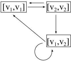
Refer to caption

Figure 5. The graph H3H_{3} for Example 4.7
Example 4.8.

We continue with Example 3.16, and illustrate how to define an order on r−1​(v1)r^{-1}(v_{1}) where v1∈V4v_{1}\in V_{4}, if (fv1,v1(4),fv1,v2(4),fv1,v3(4),fv1,v4(4))=(4,2,2,3)(f_{v_{1},v_{1}}^{(4)},f_{v_{1},v_{2}}^{(4)},f_{v_{1},v_{3}}^{(4)},f_{v_{1},v_{4}}^{(4)})=(4,2,2,3). In what follows we drop the superscript (4)(4). The graph ℋ=ℋ4\mathcal{H}=\mathcal{H}_{4} is shown in Figure 6; recall that v1∈[v1,v1]v_{1}\in[v_{1},v_{1}], v2∈[v2,v1]v_{2}\in[v_{2},v_{1}], v3∈[v2,v2]v_{3}\in[v_{2},v_{2}] and v4∈[v3,v3]v_{4}\in[v_{3},v_{3}]. The (nontrivial part of the) system of relations (4.7) become

f~v1,v1=f~v1,v1,v2+f~v1,v1,v3​ and ​f~v1,v2=f~v1,v2,v2+f~v1,v2,v3,\widetilde{f}_{v_{1},v_{1}}=\widetilde{f}_{v_{1},v_{1},v_{2}}+\widetilde{f}_{v_{1},v_{1},v_{3}}\mbox{ and }\widetilde{f}_{v_{1},v_{2}}=\widetilde{f}_{v_{1},v_{2},v_{2}}+\widetilde{f}_{v_{1},v_{2},v_{3}},

and the balance relations (4.8) become, with v¯=v1,v2\overline{v}=v_{1},\,\,v_{2} and v3v_{3}

f~v1,v4=f¯v1,v1,f~v1,v1,v2+f~v1,v2,v2=f¯v1,v3+f¯v1,v2​ and ​f~v1,v1,v3+f~v1,v3+f~v1,v2,v3=f¯v1,v4\widetilde{f}_{v_{1},v_{4}}=\overline{f}_{v_{1},v_{1}},\,\,\widetilde{f}_{v_{1},v_{1},v_{2}}+\widetilde{f}_{v_{1},v_{2},v_{2}}=\overline{f}_{v_{1},v_{3}}+\overline{f}_{v_{1},v_{2}}\mbox{ and }\widetilde{f}_{v_{1},v_{1},v_{3}}+\widetilde{f}_{v_{1},v_{3}}+\widetilde{f}_{v_{1},v_{2},v_{3}}=\overline{f}_{v_{1},v_{4}}

respectively. If we let

f~v1,v1=f~v1,v1,v2+f~v1,v1,v3=2+1​ and ​f~v1,v2=f~v1,v2,v2+f~v1,v2,v3=2+0,\widetilde{f}_{v_{1},v_{1}}=\widetilde{f}_{v_{1},v_{1},v_{2}}+\widetilde{f}_{v_{1},v_{1},v_{3}}=2+1\mbox{ and }\widetilde{f}_{v_{1},v_{2}}=\widetilde{f}_{v_{1},v_{2},v_{2}}+\widetilde{f}_{v_{1},v_{2},v_{3}}=2+0,

then the balance relations are satisfied. A valid choice of an ordering on r−1​(v1)r^{-1}(v_{1}) obtained using our algorithm is w⁡(v1,3,4)=v1​v22​v3​v4​v1​v3​v4​v1​v4​v1w(v_{1},3,4)=v_{1}v_{2}^{2}v_{3}v_{4}v_{1}v_{3}v_{4}v_{1}v_{4}v_{1}; the other is w⁡(v1,3,4)=v1​v22​v3​v4​v1​v4​v1​v3​v4​v1w(v_{1},3,4)=v_{1}v_{2}^{2}v_{3}v_{4}v_{1}v_{4}v_{1}v_{3}v_{4}v_{1}. Note that there are other valid choices of orderings on r−1​(v1)r^{-1}(v_{1}), but they are not achieved with this algorithm.
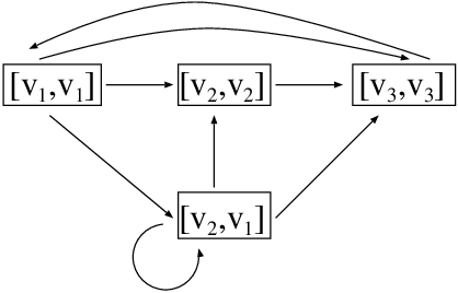
Refer to caption

Figure 6. The graph H4H_{4} for Example 4.8

As a corollary we identify the conditions needed so that a perfect order in 𝒫B∗\mathcal{P}^{*}_{B} is supported by BB. Note that one can talk of a skeleton and correspondence ℱ\mathcal{F} and σ\sigma of being capable of generating orders that belong to 𝒫B∗\mathcal{P}_{B}^{*}: either all perfect orders ω\omega having skeleton (ℱ,σ)(\mathcal{F},\sigma) belong to 𝒫B∗\mathcal{P}_{B}^{*}, or none of them do.

Corollary 4.9.

Let BB be a Bratteli diagram with incidence matrices (Fn)(F_{n}). Let ℱ\mathcal{F} be a skeleton on BB and σ\sigma an associated correspondence that can generate orders in 𝒫B∗\mathcal{P}_{B}^{*}, and suppose that all associated graphs ℋn\mathcal{H}_{n} are positively strongly connected. Suppose also that for each MM (and hence each sequence (v~n=vn​(M))(\widetilde{v}_{n}=v_{n}(M))), there exists an n0n_{0} such that for any n≥n0n\geq n_{0}, any m>nm>n, and any u∈Vmu\in V_{m}, the entries of incidence matrices (Fn)(F_{n}) satisfy condition (4.9). Then there is a perfect ordering ω\omega on BB such that ℱ=ℱω\mathcal{F}=\mathcal{F}_{\omega} and the Vershik map φω\varphi_{\omega} satisfies the relation φω=σ\varphi_{\omega}=\sigma on Xmax​(ℱ)X_{\max}(\mathcal{F}).

In the remaining part of this section, we will consider the class of Bratteli diagrams 𝒜\mathcal{A} that is close, by its structure, to diagrams of finite rank. We refer to the notation in Definition 2.2.

Take a Bratteli diagram BB and let the columns of An(i)A_{n}^{(i)} be indexed by vertices Vn(i)V_{n}^{(i)}. Define XB(i)={x=(xn)∈XB:s⁡(xn)∈Vn(i)​ for each ​n}X_{B}^{(i)}=\{x=(x_{n})\in X_{B}:s(x_{n})\in V_{n}^{(i)}\mbox{ for each }n\}, and let XB(a)=XB\⋃iXB(i)X_{B}^{(a)}=X_{B}\backslash\bigcup_{i}X_{B}^{(i)}. We will call XB(i)X_{B}^{(i)} the ii-th minimal component of XBX_{B} (here minimality is considered with respect to the tail equivalence relation ℰ\mathcal{E}). If B∈𝒜B\in\mathcal{A}, and has incidence matrices of the form as in (2.1) we will say that BB has kk minimal components.

Given a skeleton ℱ\mathcal{F} on BB, let Xmax(i)​(ℱ)=Xmax​(ℱ)∩XB(i)X_{\max}^{(i)}(\mathcal{F})=X_{\max}(\mathcal{F})\cap X_{B}^{(i)}; define Xmin(i)​(ℱ)X_{\min}^{(i)}(\mathcal{F}) similarly. Also, if ω\omega is an order on BB, define Xmax(i)​(ω)X_{\max}^{(i)}(\omega) and Xmin(i)​(ω)X_{\min}^{(i)}(\omega) analogously. Note that for any statement that we make about a skeleton, we can make an analogous statement about an order - simply consider the skeleton associated with the well-telescoped order.

The following lemma is straightforward.

Lemma 4.10.

Let B∈𝒜B\in\mathcal{A}. Then

  1. (1)

    If ℱ\mathcal{F} is a skeleton on BB, then, for each ii, the sets Xmax(i)​(ℱ)X_{\max}^{(i)}(\mathcal{F}) and Xmin(i)​(ℱ)X_{\min}^{(i)}(\mathcal{F}) are closed.

  2. (2)

    If ω\omega is a perfect order on BB, then, for each ii, φω:Xmax(i)​(ω)→Xmin(i)​(ω)\varphi_{\omega}:X_{\max}^{(i)}(\omega)\rightarrow X_{\min}^{(i)}(\omega) is a homeomorphism.

We use Proposition 3.23 to prove the following generalization of Proposition 3.26 in [BKY13].

Proposition 4.11.

Let B∈𝒜B\in\mathcal{A} have kk minimal components. Suppose that CnC_{n} is a d×dd\times d matrix where 1≤d≤k−11\leq d\leq k-1. If k=2k=2, then there are perfect orderings on BB only if Cn=(1)C_{n}=(1) for all but finitely many nn. If k>2k>2, then there is no perfect ordering on BB.

Proof.

We first claim that in ℋn\mathcal{H}_{n}, there are kk connected components of vertices Tn(1),…​Tn(k)T_{n}^{(1)},\ldots T_{n}^{(k)}, such that there are no edges from vertices in Tn(i)T_{n}^{(i)} to vertices in Tn(j)T_{n}^{(j)} if i≠ji\neq j. To see this, if 1≤i≤k1\leq i\leq k, let Tn(i)={[v¯,v~,n]:v¯∈Vn(i),v~∈Vn(i)}T_{n}^{(i)}=\{[\overline{v},\widetilde{v},n]:\overline{v}\in V_{n}^{(i)},\widetilde{v}\in V_{n}^{(i)}\}. By Lemma 4.10, for large nn, if v~∈V~n(i)\widetilde{v}\in\widetilde{V}_{n}^{(i)} it is not possible that v¯∈σn​(v~)\overline{v}\in\sigma_{n}(\widetilde{v}) if v¯∉V¯n(i)\overline{v}\not\in\overline{V}_{n}^{(i)}.

If ω\omega is a perfect order on BB, we assume that (B,ω)(B,\omega) is well telescoped and has skeleton ℱω\mathcal{F}_{\omega}. (Otherwise we work with the diagram B′B^{\prime} on which L⁡(ω)L(\omega) is well telescoped: Note that if BB has incidence matrices of the given form, then so does any telescoping.) By Proposition 3.23, the graphs ℋn\mathcal{H}_{n} are weakly connected. The only way that this can happen is if there are k−1k-1 remaining vertices in ℋn\mathcal{H}_{n} (so that dd must equal k−1k-1), each have one incoming edge from one of the components Tn(i)T_{n}^{(i)}, and one outgoing edge into one of the components Tn(j)T_{n}^{(j)}. Each of these remaining vertices in ℋn\mathcal{H}_{n} corresponds to exactly one vertex in Vn\⋃i=1kVn(i)V_{n}\backslash\bigcup_{i=1}^{k}V_{n}^{(i)}. Thus at least one of the components, say Tn(1)T_{n}^{(1)}, has no incoming edges. Take now a vertex tt, not belonging to any of the Tn(j)T_{n}^{(j)}’s, such that if v∈tv\in t, then s⁡(e¯v)∈Tn(p)s(\overline{e}_{v})\in T_{n}^{(p)}, where p≠1p\neq 1. Since the row in FnF_{n} corresponding to vv is strictly positive, we have a contradiction as there is no path from Tn(p)T_{n}^{(p)} to Tn(1)T_{n}^{(1)}. ∎

5. The infinitesimal subgroup of diagrams that support perfect orders

We will use our results from Section 4 to give an alternative proof of the following result that was proved in [GPS95] (Corollary 2). We recall that one can associate the so called dimension group with each simple Bratteli diagram B=(V,E)B=(V,E). Let (Fn)(F_{n}) be the sequence of incidence matrices of BB, then the dimension group GG is defined as the inductive limit:

G:=lim→n→∞⁡ℤ|Vn|⟶Fnℤ|Vn+1|.G:=\varinjlim_{n\to\infty}\mathbb{Z}^{|V_{n}|}\stackrel{{\scriptstyle F_{n}}}{{\longrightarrow}}\mathbb{Z}^{|V_{n+1}|}.

For all information on dimension groups, we refer the reader to [Eff81].

If GG is a simple dimension group, the elements gg of GG of the infinitesimal subgroup I​n​f​(G)Inf(G) are defined by the relation: τ⁡(g)=0\tau(g)=0 for every normalized trace τ\tau on GG. Any normalized trace is defined by a probability measure invariant with respect to the tail equivalence relation. If B′B^{\prime} is a telescoping of BB, then their dimension groups GG, G′G^{\prime} are group order isomorphic, and this isomorphism maps I​n​f​(G)Inf(G) onto I​n​f​(G′)Inf(G^{\prime}).

Theorem 5.1.

Let BB be a simple Bratteli diagram and GG its dimension group. Suppose ω∈𝒫B∩𝒪B​(j)\omega\in\mathcal{P}_{B}\cap\mathcal{O}_{B}(j), that is there is a perfect order ω\omega on BB with exactly jj maximal paths and jj minimal paths where j≥2j\geq 2. Then I​n​f​(G)Inf(G), the infinitesimal subgroup of GG, contains a subgroup isomorphic to ℤj−1\mathbb{Z}^{j-1}.

Proof.

Given a simple Bratteli diagram BB and ω∈𝒫B∩𝒪B​(j)\omega\in\mathcal{P}_{B}\cap\mathcal{O}_{B}(j), we assume that (B,ω)(B,\omega) is well telescoped. For if not, we will telescope (B,ω)(B,\omega) to (B′,ω′)(B^{\prime},\omega^{\prime}), and working with (B′,ω′)(B^{\prime},\omega^{\prime}), we shall show that if G′G^{\prime} is the dimension group defined by B′B^{\prime}, then I​n​f​(G′)Inf(G^{\prime}) contains a subgroup isomorphic to ℤj−1\mathbb{Z}^{j-1}. Since GG, G′G^{\prime} are order isomorphic groups with the isomorphism mapping I​n​f​(G)Inf(G) to I​n​f​(G′)Inf(G^{\prime}), then I​n​f​(G)Inf(G) will also contain a subgroup isomorphic to ℤj−1\mathbb{Z}^{j-1}.

(1) In the proof, we will use the notation defined in Sections 3 and 4. This means that we will freely operate with such objects as the skeleton ℱω\mathcal{F}_{\omega}, correspondence σ=(σn)\sigma=(\sigma_{n}), sets of maximal and minimal vertices V~n,V¯n\widetilde{V}_{n},\overline{V}_{n}, partitions W​(n),W′​(n)W(n),W^{\prime}(n), sets E~​(Wv~​(n),u),E¯​(Wv¯′​(n),u)\widetilde{E}(W_{\widetilde{v}}(n),u),\overline{E}(W^{\prime}_{\overline{v}}(n),u), maximal and minimal finite paths e~v,e¯v,e~​(Vn,u),e¯​(Vn,u)\widetilde{e}_{v},\overline{e}_{v},\widetilde{e}(V_{n},u),\overline{e}(V_{n},u) (defined just before Lemma 4.2), etc.

Fix a level nn such that n>n0n>n_{0} where n0n_{0} is as in the first statement of Corollary 4.4, so that |V~i|=|V¯i|=j|\widetilde{V}_{i}|=|\overline{V}_{i}|=j for all i≥n−1i\geq n-1, and take a maximal vertex v~∗∈V~n−1\widetilde{v}^{*}\in\widetilde{V}_{n-1}. We construct a sequence of vectors (εv~∗(n+k))k≥1(\varepsilon_{\widetilde{v}^{*}}^{(n+k)})_{k\geq 1} with εv~∗(n+k)∈ℤ|Vn+k|\varepsilon_{\widetilde{v}^{*}}^{(n+k)}\in\mathbb{Z}^{|V_{n+k}|} as follows. Take first a vertex v∈Vn+1v\in V_{n+1} and set

(5.1) εv~∗(n+1)(v):={−1if s(e¯v)∈W′σn−1​(v~∗)(n),s(e~v)∉Wv~∗(n),1if s(e¯v)∉W′σn−1​(v~∗)(n),s(e~v)∈Wv~∗(n),0 otherwise \varepsilon_{\widetilde{v}*}^{(n+1)}(v):=\left\{\begin{array}[]{cc}-1&\mbox{if }s(\overline{e}_{v})\in W^{\prime}_{\sigma_{n-1}(\widetilde{v}^{*})}(n),s(\widetilde{e}_{v})\notin W_{\widetilde{v}^{*}}(n),\\ 1&\mbox{if }s(\overline{e}_{v})\notin W^{\prime}_{\sigma_{n-1}(\widetilde{v}^{*})}(n),s(\widetilde{e}_{v})\in W_{\widetilde{v}^{*}}(n),\\ 0&\mbox{ otherwise }\end{array}\right.

to obtain the vv-th entry of εv~∗(n+1)\varepsilon_{\widetilde{v}^{*}}^{(n+1)}. In general, let vv be any vertex from Vn+kV_{n+k}. Then we define εv~∗(n+k)\varepsilon_{\widetilde{v}^{*}}^{(n+k)} as follows:

(5.2) εv~∗(n+k)(v):={−1if s(e¯(Vn,v))∈W′σn−1​(v~∗)(n),s(e~(Vn,v))∉Wv~∗(n),1if s(e¯(Vn,v))∉W′σn−1​(v~∗)(n),s(e~(Vn,v))∈Wv~∗(n),0 otherwise. \varepsilon_{\widetilde{v}*}^{(n+k)}(v):=\left\{\begin{array}[]{cc}-1&\mbox{if }s(\overline{e}(V_{n},v))\in W^{\prime}_{\sigma_{n-1}(\widetilde{v}^{*})}(n),s(\widetilde{e}(V_{n},v))\notin W_{\widetilde{v}^{*}}(n),\\ 1&\mbox{if }s(\overline{e}(V_{n},v))\notin W^{\prime}_{\sigma_{n-1}(\widetilde{v}^{*})}(n),s(\widetilde{e}(V_{n},v))\in W_{\widetilde{v}^{*}}(n),\\ 0&\mbox{ otherwise. }\end{array}\right.

(2) We will show that for any k≥1k\geq 1

(5.3) Fn+kεv~∗(n+k)=εv~∗(n+k+1).F_{n+k}\varepsilon_{\widetilde{v}*}^{(n+k)}=\varepsilon_{\widetilde{v}*}^{(n+k+1)}.

To prove (5.3), we use another representation of entries of the vector εv~∗(n+k)(v)\varepsilon_{\widetilde{v}*}^{(n+k)}(v). Indeed, since ω\omega is perfect we have that relation (4.9) in Section 4 holds. Also, if F(n,n+k)=Fn+k−1∘⋯∘Fn,k≥1F(n,n+k)=F_{n+k-1}\circ\cdots\circ F_{n},k\geq 1, and u∈Vn+ku\in V_{n+k}, then relation (4.9) becomes

∑w∈Wv~​(n)f~u,w(n,n+k)=∑w′∈Wσn−1​(v~)′​(n)f¯u,w′(n,n+k),u∈Vn+k.\sum_{w\in W_{\widetilde{v}}(n)}\widetilde{f}_{u,w}^{(n,n+k)}=\sum_{w^{\prime}\in W^{\prime}_{\sigma_{n-1}(\widetilde{v})}(n)}\overline{f}_{u,w^{\prime}}^{(n,n+k)},\ \ \ \ u\in V_{n+k}\,.

It is straightforward to check that

(5.4) εv~∗(n+k)(v)=∑w∈Wv~∗​(n)fv,w(n,n+k)−∑w′∈Wσn−1​(v~∗)′​(n)fv,w′(n,n+k),v∈Vn+k.\varepsilon_{\widetilde{v}*}^{(n+k)}(v)=\sum_{w\in W_{\widetilde{v}^{*}}(n)}f^{(n,n+k)}_{v,w}-\sum_{w^{\prime}\in W^{\prime}_{\sigma_{n-1}(\widetilde{v}^{*})}(n)}f^{(n,n+k)}_{v,w^{\prime}},\ \ v\in V_{n+k}.

Then (5.3) can be proved by induction. Indeed, compute for k=1k=1

Fn+1εv~∗(n+1)(v)\displaystyle F_{n+1}\varepsilon_{\widetilde{v}*}^{(n+1)}(v) =\displaystyle= ∑u∈Vn+1fv,u(n+1)​(∑w∈Wv~∗​(n)fu,w(n)−∑w′∈Wσn−1​(v~∗)′​(n)fu,w′(n))\displaystyle\sum_{u\in V_{n+1}}f^{(n+1)}_{v,u}\left(\sum_{w\in W_{\widetilde{v}^{*}}(n)}f^{(n)}_{u,w}-\sum_{w^{\prime}\in W^{\prime}_{\sigma_{n-1}(\widetilde{v}^{*})}(n)}f^{(n)}_{u,w^{\prime}}\right)
=\displaystyle= ∑w∈Wv~∗​(n)fv,w(n,n+2)−∑w′∈Wσn−1​(v~∗)′​(n)fv,w′(n,n+2)\displaystyle\sum_{w\in W_{\widetilde{v}^{*}}(n)}f^{(n,n+2)}_{v,w}-\sum_{w^{\prime}\in W^{\prime}_{\sigma_{n-1}(\widetilde{v}^{*})}(n)}f^{(n,n+2)}_{v,w^{\prime}}
=\displaystyle= εv~∗(n+2)(v),v∈Vn+2.\displaystyle\varepsilon_{\widetilde{v}*}^{(n+2)}(v),\ \ v\in V_{n+2}.

The induction step can be computed in a similar way. We omit the details.

(3) It follows from relation (5.3) that every vector εv~∗(n+1),v~∗∈V~n−1,\varepsilon_{\widetilde{v}^{*}}^{(n+1)},\widetilde{v}^{*}\in\widetilde{V}_{n-1}, generates the element gv~∗=(εv~∗(n+1),εv~∗(n+2),εv~∗(n+3),…)g_{\widetilde{v}^{*}}=(\varepsilon_{\widetilde{v}^{*}}^{(n+1)},\varepsilon_{\widetilde{v}^{*}}^{(n+2)},\varepsilon_{\widetilde{v}^{*}}^{(n+3)},\ldots) of the dimension group GG of BB.

Next, since W⁡(n)W(n) and W′​(n)W^{\prime}(n) constitute partitions of VnV_{n}, we have

∑v~∈V~n−1εv~(n+k)​(v)\displaystyle\sum_{\widetilde{v}\in\widetilde{V}_{n-1}}\varepsilon^{(n+k)}_{\widetilde{v}}(v) =\displaystyle= ∑v~∈V~n−1(∑w∈Wv~∗​(n)fv,w(n,n+k)−∑w′∈Wσn−1​(v~∗)′​(n)fv,w′(n,n+k))\displaystyle\sum_{\widetilde{v}\in\widetilde{V}_{n-1}}\left(\sum_{w\in W_{\widetilde{v}^{*}}(n)}f^{(n,n+k)}_{v,w}-\sum_{w^{\prime}\in W^{\prime}_{\sigma_{n-1}(\widetilde{v}^{*})}(n)}f^{(n,n+k)}_{v,w^{\prime}}\right)
=\displaystyle= ∑w∈Vnfv,w(n,n+k)−∑w′∈Vnfv,w′(n,n+k)\displaystyle\sum_{w\in V_{n}}f^{(n,n+k)}_{v,w}-\sum_{w^{\prime}\in V_{n}}f^{(n,n+k)}_{v,w^{\prime}}
=\displaystyle= 0\displaystyle 0

for any kk and vv. That is the vectors {εv~(n+k):v~∈V~n−1}\{\varepsilon^{(n+k)}_{\widetilde{v}}:\widetilde{v}\in\widetilde{V}_{n-1}\} are linearly dependent.

On the other hand, we claim that any subset of this set containing j−1j-1 vectors is linearly independent over ℤ\mathbb{Z}. To simplify our notation we consider the set of vectors {εv~(n+1):v~∈V~n−1}\{\varepsilon^{(n+1)}_{\widetilde{v}}:\widetilde{v}\in\widetilde{V}_{n-1}\} only, since the case for the vectors {εv~(n+k):v~∈V~n−1}\{\varepsilon^{(n+k)}_{\widetilde{v}}:\widetilde{v}\in\widetilde{V}_{n-1}\} where k>1k>1 is considered similarly. Suppose that V~n−1={v~1,…,v~j}.\widetilde{V}_{n-1}=\{\widetilde{v}_{1},\ldots,\widetilde{v}_{j}\}. Consider the |Vn+1|×j|V_{n+1}|\times j-matrix whose ii-th column is the vector εv~i(n+1)\varepsilon^{(n+1)}_{\widetilde{v}_{i}}. We fix a vertex u∈Vn+1u\in V_{n+1} and look at the uu-th row RuR_{u} of this matrix; this is the row formed by the uu-th entries of the vectors {εv~i(n+1)},1≤i≤j\{\varepsilon^{(n+1)}_{\widetilde{v}_{i}}\},1\leq i\leq j. The definition of the entries of the row RuR_{u} (see (5.1)) shows that either they are all 0 or each value 1 and −1-1 is taken exactly once, and all remaining entries in this row are zero. Note that since this property holds for any vertex uu, we have another proof of the fact that the sum of all vectors {εv~(n+1)}\{\varepsilon^{(n+1)}_{\widetilde{v}}\} is zero. Also, for every v~\widetilde{v}, the strong connectivity of the graph ℋn\mathcal{H}_{n} implies that we have |{u∈Vn+1:εu,v~(n+1)=1}|≥1|\{u\in V_{n+1}:\varepsilon_{u,\widetilde{v}}^{(n+1)}=1\}|\geq 1 and |{u∈Vn+1:εu,v~(n+1)=−1}|≥1|\{u\in V_{n+1}:\varepsilon_{u,\widetilde{v}}^{(n+1)}=-1\}|\geq 1 (but these sets may be of different cardinalities).

We pick any vector εv~(n+1)\varepsilon_{\widetilde{v}}^{(n+1)} in the set {εv~i(n+1)}\{\varepsilon^{(n+1)}_{\widetilde{v}_{i}}\} and show that the set of remaining vectors {εv~i(n+1)}∖εv~(n+1)\{\varepsilon^{(n+1)}_{\widetilde{v}_{i}}\}\setminus\varepsilon_{\widetilde{v}}^{(n+1)} is linearly independent. Indeed, assume that

(5.5) ∑v~i≠v~mv~i​εv~i(n+1)=0;\sum_{\widetilde{v}_{i}\neq\widetilde{v}}m_{\widetilde{v}_{i}}\varepsilon^{(n+1)}_{\widetilde{v}_{i}}=0;

we shall show that all mvim_{v_{i}}’s in (5.5) must be equal to mm. If one assumes that m≠0m\neq 0 we obtain two contradictory equalities ∑v~≠v~0εv~(n+1)=0\sum_{\widetilde{v}\neq\widetilde{v}_{0}}\varepsilon^{(n+1)}_{\widetilde{v}}=0 and ∑v~≠v~0εv~(n+1)=−εv~0(n+1)\sum_{\widetilde{v}\neq\widetilde{v}_{0}}\varepsilon^{(n+1)}_{\widetilde{v}}=-\varepsilon^{(n+1)}_{\widetilde{v}_{0}}. Pick any two maximal vertices v~p\widetilde{v}_{p} and v~t\widetilde{v}_{t} that are not equal to v~\widetilde{v}. Firstly, by the strong connectivity of ℋn\mathcal{H}_{n}, there exist vertices [v¯p,v~p][\overline{v}_{p},\widetilde{v}_{p}] and [v¯t,v~t][\overline{v}_{t},\widetilde{v}_{t}] in ℋn\mathcal{H}_{n} that do not have loops. Secondly, also by the strong connectivity of ℋn\mathcal{H}_{n}, we can find a path from [v¯p,v~p][\overline{v}_{p},\widetilde{v}_{p}] to [v¯t,v~t][\overline{v}_{t},\widetilde{v}_{t}] , and we can also assume that for any vertex along this path, there are no loops (otherwise these vertices can be removed from the path, and we still have a valid path). Finally, note that if there is an edge from [v¯′,v~′][\overline{v}^{\prime},\widetilde{v}^{\prime}] to [v¯∗,v~∗][\overline{v}^{*},\widetilde{v}^{*}] and there is no loop at [v¯∗,v~∗][\overline{v}^{*},\widetilde{v}^{*}], then mv~∗=mv~′m_{\widetilde{v}^{*}}=m_{\widetilde{v}^{\prime}}. The result follows.

(4) It remains to show that the elements gv~,v~∈V~n−1,g_{\widetilde{v}},\widetilde{v}\in\widetilde{V}_{n-1}, belong to the infinitesimal subgroup I​n​f​(G)Inf(G). Since GG is a simple dimension group, it suffices to check that τ⁡(gv~)=0\tau(g_{\widetilde{v}})=0 for any trace τ\tau on GG or, equivalently, for any invariant measure μ\mu.

Fix a probability φω\varphi_{\omega}-invariant measure μ\mu on the path space of the diagram BB. Consider the vector p(n)=(pv(n))∈ℝ|Vn|p^{(n)}=(p_{v}^{(n)})\in\mathbb{R}^{|V_{n}|} whose entries are μ\mu-measures of a finite path (cylinder set) with source v0v_{0} and range vv. This means that, in particular, μ⁡(e~​(v0,w))=pw(n),w∈Wv~​(n)\mu(\widetilde{e}(v_{0},w))=p_{w}^{(n)},w\in W_{\widetilde{v}}(n) and μ⁡(e¯​(v0,w′))=pw′(n),w′∈Wσn−1​(v~)​(n)\mu(\overline{e}(v_{0},w^{\prime}))=p_{w^{\prime}}^{(n)},w^{\prime}\in W_{\sigma_{n-1}(\widetilde{v})}(n). As noticed in [BKMS10], we have FnT​p(n+1)=p(n),∀n∈ℕ,F_{n}^{T}p^{(n+1)}=p^{(n)},\forall n\in\mathbb{N}, or

∑v∈Vn+1fv,w(n)​pv(n+1)=pw(n),w∈Vn.\sum_{v\in V_{n+1}}f_{v,w}^{(n)}p_{v}^{(n+1)}=p^{(n)}_{w},\ \ w\in V_{n}.

Compute <p(n+1),εv~(n+1)><p^{(n+1)},\varepsilon^{(n+1)}_{\widetilde{v}}> where <⋅,⋅><\cdot,\cdot> is the inner product:

<p(n+1),εv~(n+1)>\displaystyle<p^{(n+1)},\varepsilon^{(n+1)}_{\widetilde{v}}> =\displaystyle= <Fn+1T​p(n+2),εv~(n+1)>\displaystyle<F_{n+1}^{T}p^{(n+2)},\varepsilon^{(n+1)}_{\widetilde{v}}>
=\displaystyle= <p(n+2),Fn+1​εv~(n+1)>\displaystyle<p^{(n+2)},F_{n+1}\varepsilon^{(n+1)}_{\widetilde{v}}>
=\displaystyle= <p(n+2),εv~(n+2)>\displaystyle<p^{(n+2)},\varepsilon^{(n+2)}_{\widetilde{v}}>
⋯\displaystyle\cdots
=\displaystyle= <p(n+j),εv~(n+j)>\displaystyle<p^{(n+j)},\varepsilon^{(n+j)}_{\widetilde{v}}>

for any jj. On the other hand,

<p(n+1),εv~(n+1)>\displaystyle<p^{(n+1)},\varepsilon^{(n+1)}_{\widetilde{v}}> =\displaystyle= ∑v∈Vn+1pv(n+1)​(∑w∈Wv~​(n)fv,w(n)−∑w′∈Wσn−1​(v~)′​(n)fv,w′(n))\displaystyle\sum_{v\in V_{n+1}}p_{v}^{(n+1)}\left(\sum_{w\in W_{\widetilde{v}}(n)}f_{v,w}^{(n)}-\sum_{w^{\prime}\in W^{\prime}_{\sigma_{n-1}(\widetilde{v})}(n)}f_{v,w^{\prime}}^{(n)}\right)
=\displaystyle= ∑w∈Wv~​(n)∑v∈Vn+1fv,w(n)​pv(n+1)−∑w′∈Wσn−1​(v~)′​(n)∑v∈Vn+1fv,w′(n)​pv(n+1)\displaystyle\sum_{w\in W_{\widetilde{v}}(n)}\sum_{v\in V_{n+1}}f_{v,w}^{(n)}p_{v}^{(n+1)}-\sum_{w^{\prime}\in W^{\prime}_{\sigma_{n-1}(\widetilde{v})}(n)}\sum_{v\in V_{n+1}}f_{v,w^{\prime}}^{(n)}p_{v}^{(n+1)}
=\displaystyle= ∑w∈Wv~​(n)pw(n)−∑w′∈Wσn−1​(v~)′​(n)pw′(n)\displaystyle\sum_{w\in W_{\widetilde{v}}(n)}p_{w}^{(n)}-\sum_{w^{\prime}\in W^{\prime}_{\sigma_{n-1}(\widetilde{v})}(n)}p_{w^{\prime}}^{(n)}
=\displaystyle= 0\displaystyle 0

because

∑w∈Wv~​(n)pw(n)\displaystyle\sum_{w\in W_{\widetilde{v}}(n)}p_{w}^{(n)} =\displaystyle= μ⁡(⋃w∈Wv~​(n)e~​(v0,w))\displaystyle\mu(\bigcup_{w\in W_{\widetilde{v}}(n)}\widetilde{e}(v_{0},w))
=\displaystyle= μ⁡(φω​(⋃w∈Wv~​(n)e~​(v0,w)))\displaystyle\mu(\varphi_{\omega}(\bigcup_{w\in W_{\widetilde{v}}(n)}\widetilde{e}(v_{0},w)))
=\displaystyle= μ⁡(⋃w′∈Wσn−1​(v~)′​(n)e¯​(v0,w′))\displaystyle\mu(\bigcup_{w^{\prime}\in W^{\prime}_{\sigma_{n-1}(\widetilde{v})}(n)}\overline{e}(v_{0},w^{\prime}))
=\displaystyle= ∑w′∈Wσn−1​(v~)′​(n)pw′(n).\displaystyle\sum_{w^{\prime}\in W^{\prime}_{\sigma_{n-1}(\widetilde{v})}(n)}p_{w^{\prime}}^{(n)}.

This proves that gv~∈I​n​f​(G)g_{\widetilde{v}}\in Inf(G). ∎

Remark 5.2.

In the simpler case when BB is of finite rank, then for each nn, εv~∗(n)=εv~∗\varepsilon_{\widetilde{v}*}^{(n)}=\varepsilon_{\widetilde{v}*}, each of the latter jj vectors correspond to an infinitesimal, and εv~∗=−∑v~≠v~∗εv~\varepsilon_{\widetilde{v}*}=-\sum_{\widetilde{v}\neq\widetilde{v}*}\varepsilon_{\widetilde{v}}, while {εv~:v~≠v~∗}\{\varepsilon_{\widetilde{v}}:\widetilde{v}\neq\widetilde{v}*\} is a linearly independent set, so that there are j−1j-1 identified copies of ℤ\mathbb{Z} in the infinitesimal subgroup of d​i​m​(B)dim(B).

Example 5.3.

Let

(5.6) Fn=(fa​a(n)fa​b(n)α(n)α(n)fb​a(n)fb​b(n)β(n)β(n)fc​a(n)fc​b(n)γ(n)+1γ(n)fd​a(n)fd​b(n)δ(n)δ(n)+1);F_{n}=\left(\begin{array}[]{cccc}f_{aa}^{(n)}&f_{ab}^{(n)}&\alpha^{(n)}&\alpha^{(n)}\\ f_{ba}^{(n)}&f_{bb}^{(n)}&\beta^{(n)}&\beta^{(n)}\\ f_{ca}^{(n)}&f_{cb}^{(n)}&\gamma^{(n)}+1&\gamma^{(n)}\\ f_{da}^{(n)}&f_{db}^{(n)}&\delta^{(n)}&\delta^{(n)}+1\\ \end{array}\right);

then there exist orders ω\omega on BB that belong to 𝒫B∩𝒪B​(2)\mathcal{P}_{B}\cap\mathcal{O}_{B}(2), and such that the associated graph and correspondence is as in Figure 1, where a∈[a,a],a\in[a,a], b∈[b,b]b\in[b,b], c∈[a,b]c\in[a,b] and d∈[b,a]d\in[b,a]. In this case,

(5.7) εa=(00−11)​ and ​εb=(001−1);\varepsilon_{a}=\left(\begin{array}[]{c}0\\ 0\\ -1\\ 1\\ \end{array}\right)\mbox{ and }\varepsilon_{b}=\left(\begin{array}[]{cccc}0\\ 0\\ 1\\ -1\\ \end{array}\right);

so that Fn​εa=εaF_{n}\varepsilon_{a}=\varepsilon_{a} as claimed and εa\varepsilon_{a} corresponds to an element of I​n​f​(G)Inf(G).

Example 5.4.

One can vary the given skeleton and correspondence in Theorem 5.1 to maximize the number of copies of ℤ\mathbb{Z} that one can find in I​n​f​(G)Inf(G). For example, if a finite rank simple diagram BB supports orders in ω∈𝒫B​(2)\omega\in\mathcal{P}_{B}(2) that can have either of the two possible graphs described in Example 3.4, this means that there is a copy of ℤ×ℤ\mathbb{Z}\times\mathbb{Z} in I​n​f​(G)Inf(G). The incidence matrices of this diagram must have a very restrictive structure. For example, if BB has rank 4, then the incidence matrices must be of the form

(5.8) Fn=(an(1)+1an(1)an(2)an(2)bn(1)bn(1)+1bn(2)bn(2)cn(1)cn(1)cn(2)+1cn(2)dn(1)dn(1)dn(2)dn(2)+1)F_{n}=\left(\begin{array}[]{cccc}a_{n}^{(1)}+1&a_{n}^{(1)}&a_{n}^{(2)}&a_{n}^{(2)}\\ b_{n}^{(1)}&b_{n}^{(1)}+1&b_{n}^{(2)}&b_{n}^{(2)}\\ c_{n}^{(1)}&c_{n}^{(1)}&c_{n}^{(2)}+1&c_{n}^{(2)}\\ d_{n}^{(1)}&d_{n}^{(1)}&d_{n}^{(2)}&d_{n}^{(2)}+1\\ \end{array}\right)

Bratteli diagrams with these incidence matrices have 2 orders in 𝒫B∩𝒪B​(2)\mathcal{P}_{B}\cap\mathcal{O}_{B}(2), each with a different associated graph ℋ\mathcal{H}. This implies that they have (at least) two independent infinitesimals, corresponding to the elements.

(5.9) ε=(00−11)​ and ​ε′=(1−100).\varepsilon=\left(\begin{array}[]{c}0\\ 0\\ -1\\ 1\\ \end{array}\right)\mbox{ and }\varepsilon^{\prime}=\left(\begin{array}[]{cccc}1\\ -1\\ 0\\ 0\\ \end{array}\right).

Next we extend Theorem 5.1 to diagrams supporting perfect orders that belong to 𝒫B∗\mathcal{P}_{B}^{*}. This result overlaps Corollary 3 in [GPS95].

Theorem 5.5.

Let BB be a simple Bratteli diagram and GG its dimension group. Suppose ω\omega belongs to 𝒫B∗\⋃j=1∞𝒪B​(j){\mathcal{P}_{B}^{*}}\backslash\bigcup_{j=1}^{\infty}\mathcal{O}_{B}(j). Then I​n​f​(G)Inf(G), the infinitesimal subgroup of GG, contains as a subgroup the free abelian group on countably many generators.

Proof.

The proof is similar to that of Theorem 5.1. The second statement of Corollary 4.4 tells us that for each maximal path MM, with v~n=vn​(M)\widetilde{v}_{n}=v_{n}(M), there exists some level n0n_{0} such that if n≥n0−1n\geq n_{0}-1, σn​(v~n)\sigma_{n}(\widetilde{v}_{n}) is a singleton. We construct a sequence of vectors (εM(n0+k))k≥1(\varepsilon_{M}^{(n_{0}+k)})_{k\geq 1} with εM(n+k)∈ℤ|Vn+k|\varepsilon_{M}^{(n+k)}\in\mathbb{Z}^{|V_{n+k}|} as follows. Take first a vertex v∈Vn0+1v\in V_{n_{0}+1} and set

εM(n0+1)​(v):={−1if s(e¯v)∈W′σn0−1​(v~n0−1)(n0),s(e~v)∉Wv~n0−1(n0),1if s(e¯v)∉W′σn0−1​(v~n0−1)(n0),s(e~v)∈Wv~n0−1(n0),0 otherwise \varepsilon_{M}^{(n_{0}+1)}(v):=\left\{\begin{array}[]{cc}-1&\mbox{if }s(\overline{e}_{v})\in W^{\prime}_{\sigma_{n_{0}-1}(\widetilde{v}_{n_{0}-1})}(n_{0}),s(\widetilde{e}_{v})\notin W_{\widetilde{v}_{n_{0}-1}}(n_{0}),\\ 1&\mbox{if }s(\overline{e}_{v})\notin W^{\prime}_{\sigma_{n_{0}-1}(\widetilde{v}_{n_{0}-1})}(n_{0}),s(\widetilde{e}_{v})\in W_{\widetilde{v}_{n_{0}-1}}(n_{0}),\\ 0&\mbox{ otherwise }\end{array}\right.

to obtain the vv-th entry of εM(n0+1)\varepsilon_{M}^{(n_{0}+1)}. In general, let vv be any vertex from Vn0+kV_{n_{0}+k}. Then we define εM(n0+k)\varepsilon_{M}^{(n_{0}+k)} as follows:

εv~∗(n0+k)(v):={−1if s(e¯(Vn0,v))∈W′σn0−1​(v~n0−1)(n0),s(e~(Vn0,v))∉Wv~n0−1(n0),1if s(e¯(Vn0,v))∉W′σn0−1​(v~n0−1)(n0),s(e~(Vn0,v))∈Wv~n0−1(n0),0 otherwise. \varepsilon_{\widetilde{v}*}^{(n_{0}+k)}(v):=\left\{\begin{array}[]{cc}-1&\mbox{if }s(\overline{e}(V_{n_{0}},v))\in W^{\prime}_{\sigma_{n_{0}-1}(\widetilde{v}_{n_{0}-1})}(n_{0}),s(\widetilde{e}(V_{n_{0}},v))\notin W_{\widetilde{v}_{n_{0}-1}}(n_{0}),\\ 1&\mbox{if }s(\overline{e}(V_{n_{0}},v))\notin W^{\prime}_{\sigma_{n_{0}-1}(\widetilde{v}_{n_{0}-1})}(n_{0}),s(\widetilde{e}(V_{n_{0}},v))\in W_{\widetilde{v}_{n_{0}-1}}(n_{0}),\\ 0&\mbox{ otherwise. }\end{array}\right.

As in (2) of Theorem 5.1, we can show that for any k≥1k\geq 1

(5.10) Fn0+k​εM(n0+k)=εM(n0+k+1).F_{n_{0}+k}\varepsilon_{M}^{(n_{0}+k)}=\varepsilon_{M}^{(n_{0}+k+1)}.

This means that we can define, from relation (5.10), the element gM=(εM(n0+1),εM(n0+2),εM(n0+3),…)g_{M}=(\varepsilon_{M}^{(n_{0}+1)},\varepsilon_{M}^{(n_{0}+2)},\varepsilon_{M}^{(n_{0}+3)},\ldots) of the dimension group GG of BB. In this way, we get a countably infinite collection of elements {gM:M​ maximal}\{g_{M}:M\mbox{ maximal}\}.

The argument that the collection {gM:M​ maximal}\{g_{M}:M\mbox{ maximal}\} generates a free abelian group, as the case of (3) of Theorem 5.1, depends on the strong connectivity of the graphs ℋn\mathcal{H}_{n}. Take a finite set of maximal paths (M1,…,Mk)(M_{1},...,M_{k}) and suppose that there is a linear relation

∑i=1kmi​gMi=0,\sum_{i=1}^{k}m_{i}g_{M_{i}}=0,

where the mim_{i},s are nonzero. Let v~ni=v~n​(Mi)\widetilde{v}_{n}^{i}=\widetilde{v}_{n}(M_{i}) and v¯ni=v¯n​(Mi)\overline{v}_{n}^{i}=\overline{v}_{n}(M_{i}), and choose an NN large enough so that σn​(v~ni)\sigma_{n}(\widetilde{v}_{n}^{i}) is a singleton for each n≥N−1n\geq N-1 and 1≤i≤k1\leq i\leq k. Consider the |VN+1|×k|V_{N+1}|\times k-matrix whose ii-th column is the vector εMi(N+1)\varepsilon^{(N+1)}_{M_{i}}. We fix a vertex u∈VN+1u\in V_{N+1} and look at the uu-th row RuR_{u} of this matrix; this is the row formed by the uu-th entries of the vectors {εMi(n+1)},1≤i≤k\{\varepsilon^{(n+1)}_{M_{i}}\},1\leq i\leq k. The definition of the entries of the row RuR_{u} shows that apart from at most one occurrence of 1 and of −1-1, they are all 0. Note that unlike the case in the proof of (3) of Theorem 5.1, it is possible that only one of the values 11, −1-1 appear in any row RuR_{u}. Also, for every v~\widetilde{v}, the strong connectivity of the graph ℋn\mathcal{H}_{n} implies that we have |{u∈Vn+1:εu,v~(n+1)=1}|≥1|\{u\in V_{n+1}:\varepsilon_{u,\widetilde{v}}^{(n+1)}=1\}|\geq 1 and |{u∈Vn+1:εu,v~(n+1)=−1}|≥1|\{u\in V_{n+1}:\varepsilon_{u,\widetilde{v}}^{(n+1)}=-1\}|\geq 1. The linear relation implies that ∑i=1kmi​εMi(N+1)=0.\sum_{i=1}^{k}m_{i}\varepsilon^{(N+1)}_{M_{i}}=0. It follows that if a 1 occurs in the row RuR_{u} a −1-1 must also occur; i.e. if 11 occurs in RuR_{u}, then u∈[v¯Ni,v~Nj]u\in[\overline{v}_{N}^{i},\widetilde{v}_{N}^{j}] for some 1≤i,j≤k1\leq i,\,j\leq k. Otherwise - if RuR_{u} consists only of zeros - u∈[v¯,v~]u\in[\overline{v},\widetilde{v}] with v¯∉{v¯N1,…,v¯Nk}\overline{v}\not\in\{\overline{v}_{N}^{1},\ldots,\overline{v}_{N}^{k}\} and v~∉{v~N1,…,v~Nk}\widetilde{v}\not\in\{\widetilde{v}_{N}^{1},\ldots,\widetilde{v}_{N}^{k}\}. Thus, we have partitioned ℋN+1\mathcal{H}_{N+1} into two disconnected sets of vertices, contradicting its strong connectivity.

The proof that each gMg_{M} is an infinitesimal is now very similar to part (4) of the proof of Theorem 5.1.

∎

Acknowledgements.

The authors would like to thank Christian Skau for some helpful comments. Part of this work was completed while the authors were visiting The University of Iowa (S.B.) and The Université de Picardie Jules Verne (R.Y.). We are thankful to these universities for their hospitality and support.

References

  • [BKMS10] S. Bezuglyi, J. Kwiatkowski, K. Medynets, and B. Solomyak. Invariant measures on stationary Bratteli diagrams. Ergodic Theory Dynam. Systems, 30(4):973–1007, 2010.
  • [BKY13] Sergey Bezuglyi, Jan Kwiatkowski, and Reem Yassawi. Perfect orderings on finite rank Bratteli diagrams. Canad. J. Math., to appear 2013.
  • [Eff81] Edward G. Effros. Dimensions and C∗C^{\ast}-algebras, volume 46 of CBMS Regional Conference Series in Mathematics. Conference Board of the Mathematical Sciences, Washington, D.C., 1981.
  • [GPS95] Thierry Giordano, Ian F. Putnam, and Christian F. Skau. Topological orbit equivalence and C∗C^{*}-crossed products. J. Reine Angew. Math., 469:51–111, 1995.
  • [Han13] David Handelman. Equal column sum and equal row sum dimension group realizations, 2013.
  • [HPS92] Richard H. Herman, Ian F. Putnam, and Christian F. Skau. Ordered Bratteli diagrams, dimension groups and topological dynamics. Internat. J. Math., 3(6):827–864, 1992.
  • [Med06] K. Medynets. Cantor aperiodic systems and bratteli diagrams. C. R., Math., Acad. Sci. Paris, 342(1):43–46, 2006.
  • [Put89] Ian F. Putnam. The C∗C^{*}-algebras associated with minimal homeomorphisms of the Cantor set. Pacific J. Math., 136(2):329–353, 1989.