Proton-proton diffractive collisions at ultra-high energies

The observed growth of total cross sections at preLHC energies [1] initiates studies of corresponding models such as that with a maximal increase allowed by the Froissart bound [2] or with ”heretical” power-$s$ behavior [3, 4]. The $s$-channel unitarization of scattering amplitudes actualizes the use of the Glauber approach. On account of the $s$-channel rescatterings the power-$s$ growth of amplitudes is dampened to the $(\ln^{2}s)$-type, see, for example, [5, 6, 7].

The eikonal method for the $s$-channel high-energy unitarization of the scattering amplitude was used in the Dakhno-Nikonov model [8]. The model takes into account the quark structure of colliding hadrons, the gluon origin of the input pomeron and colour screening effects in collisions. The model provided a satisfactory description of $\pi p$, $pp$, $\bar{p}p$ data for diffractive processes at preLHC energies, $\sqrt{s}\sim 0.2-1.8$ TeV.

Recent measurements at LHC (ATLAS, CMS, TOTEM collaborations) and cosmic ray data initiate further interest to $s$-channel unitarized amplitudes, see, for example, [9, 10, 11, 12, 13] and references therein.

In the present note we consider diffractive $pp$ scatterings in terms of the Dakhno-Nikonov model, concentrating our attention on the ultra-high energy asymptotic behavior. We refit data taking into account new ones in the TeV-region [14, 15]. According to the fit, this region is a pre-asymptotic one. The asymptotic behaviour starts, actually, at $10^{2}-10^{3}$ TeV.

For the ultra-high energy limit the Dakhno-Nikonov model gives for total and elastic $pp$ cross sections a $(\ln^{2}s)$-growth: $\sigma_{tot}\sim\ln^{2}s$ and $\sigma_{el}\sim\ln^{2}s$. The high energy cross sections ($\sigma_{el}$, $\sigma_{tot}$) are approaching their asymptotic values from bottom to top: $\sigma_{tot}(s)/\sigma_{tot}^{(asym)}(s)<1$; this gives the illusion of exceeding the Froissart bound (though, let us emphasize, exceeding the Froissart bound does not violate general constraints for scattering amplitudes [16]).

The model tells that differential elastic cross sections depend asymptotically on transverse momenta with realization of $\tau$-scaling $(\tau={\bf q}_{\perp}^{2}\ln^{2}s)$:

Formulae of the Dakhno-Nikonov model which are used for the calculation of $\sigma_{tot}$, $\sigma_{el}$, $d\sigma_{el}/dq^{2}_{\perp}$ are given in the next section. In section 3 we present results of the fit and predictions for ($10^{2}-10^{4}$)-TeV region.

The model is based on the hypothesis of the gluon origin of the $t$-channel forces, and these gluons form pomerons. Hadrons, mesons (two-quark composite systems) and baryons (three-quark composite systems), scatter on the pomeron cloud. It is supposed that the pomeron cloud is materialized as a low-density gas, and pomeron-pomeron interactions, as well as $t$-channel transitions $P\to PP$, $P\to PPP$ and so on, can be neglected. Consequently, the $pp$ scattering amplitude is determined by the set of diagrams shown in Fig. 1.

The pomerons are formed by effective gluons ($G$) which are massive, $\sim 700-1000$ MeV [17, 18]. The pomeron parameter $\alpha^{\prime}_{P}$ is small $\alpha^{\prime}_{P}\simeq(0.10-0.25)$ GeV^-2, that means pomerons are comparatively heavy and hard [19]. The gluon structure of the pomeron provides colour screening effects for hadron quarks [20].

Total and elastic cross sections of the model for colliding hadrons $A$ and $B$ are written as follows:

Here $dr\varphi^{2}_{A}(r)$, $dr\varphi_{B}^{2}(r)$ are the quark densities of colliding hadrons:

where ${\bf r}_{a}$ are the transverse coordinates of quarks, and $\varphi_{A}^{2}$, $\varphi_{B}^{2}$ are given by quark wave functions squared integrated over longitudinal variables. Proton and pion quark densities are determined using the corresponding form factors; such an estimation can be found, for example, in [21]. The profile-function $\chi_{AB}$ describes the interaction of quarks via pomeron exchange as follows:

Functions $S_{A,B}$ stand for the pomeron-quark interactions; they are determined by the diagrams with different couplings of the pomeron quarks:

The term $\rho({\bf b}-{\bf r}_{i})$ describes the diagram where the pomeron couples to one of the hadron quarks while the terms proportional to $\exp(-r^{2}_{ij}/r^{2}_{cs})$ are related to the diagram with the pomeron couples to two quarks of the hadron. Such a diagram is a three-reggeon graph $GGP$ where $G$ is the reggeized gluon. Functions $S_{\pi}$ and $S_{p}$ tend to zero as $|\vec{r}_{ij}|\to 0$: this is the colour screening phenomenon inherent to gluonic pomeron. For the sake of convenience, one can perform calculations in the center-mass-system of the colliding quarks, supposing that the hadron momentum is shared equally between its quarks. Then

where the vertex $g$ depends on the energy squared of the colliding quarks, $s_{qq}$:

Below $s_{0}=1$ GeV². The parametrization of $g^{2}$ corresponds to the two-pole presentation of the QCD-motivated pomeron with intercepts $\alpha(0)=1$ and $\alpha(0)=1+\Delta$.

Let us consider $pp$ scattering, specifically, the term with $qq$ interaction, see Eqs. (4), (6):

Equations depend on the transverse coordinates of quarks, though the original expressions depend on the fractions of the momenta of the colliding hadrons carried by the quark, $x_{i}$. In the functions $S_{\pi}$, $S_{p}$ we put $x_{i}=1/2$ for a meson and $x_{i}=1/3$ for the proton, in other words we assume that hadron wave functions $\varphi_{A}(r,x)$ and $\varphi_{B}(r,x)$ select the mean values of $x_{i}$ in the interaction blocks. So, in the used equations we put $s_{qq}=s/9$ for $pp$ collisions and perform the renormalization of the value $G$ by including the factor $\alpha^{\prime}_{P}\ln{9}$ that can lead to $G<0$. Of course, the slope parameter $2G+\alpha^{\prime}_{P}\ln{s}$ should be positive in the region of application of the model.

The Dakhno-Nikonov model is actually a realization of the Good-Walker eikonal approach [22] for a continual set of channels (each quark configuration with fixed coordinates is a separate channel). Used in the model the two-pole pomeron exchange is popular from the sixties till now, see for example ref. [23].

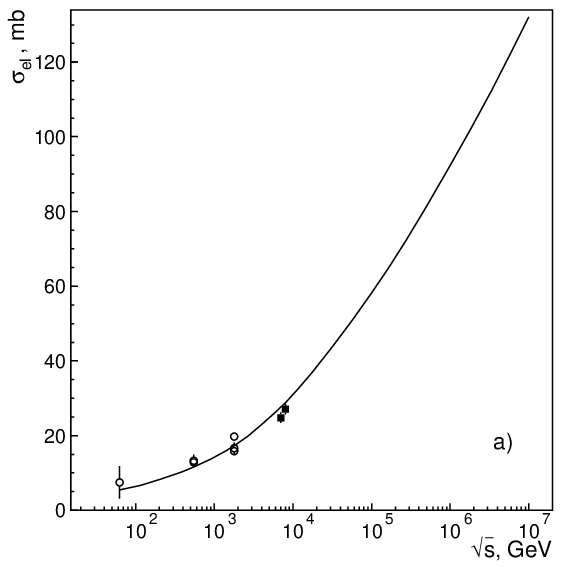
Figs. 2-4 demonstrate fit results of the diffractive scattering $pp$ data, including those at LHC energies [14] and cosmic ray ones [15]. In Fig. 2 we show total and inelastic cross sections, the fit gives a good approximation to data at $\sqrt{s}\sim 50-5\cdot 10^{4}$ GeV and a prediction for the region $\sqrt{s}\sim 10^{5}-10^{7}$ GeV. The same level of description demonstrates us $\sigma_{el}$ and the slope $B$, see Fig. 3.

In Fig. 4a we show $d\sigma_{el}/d{\bf q}^{2}_{\perp}$ at ISR and LHC energies and their fit, and Fig. 4b demonstrates the profile function $T(b)$ determined as

Obtained in the fit the profile functions $T(b)$, which are given by Eq. (9), are shown in Fig. 4b for preLHC, LHC and ultra-high energies. It is seen that the profile function saturation mode, $T(b)\to 1$, works at ultra-high energies ($100-1000$ TeV), at LHC energies the saturation mode is only starting.

Parameters of the present fit and that of ref. [8] approximately coincide:

The only change is in the value of $\alpha^{\prime}_{P}$, we observe the decrease of $\alpha^{\prime}_{P}$ that means the slowing of the asymptotic regime switch-on.

At $\ln s>>1$, when the asymptotic regime works, there are well-seen two regions in the $b$-space (Fig. 4b): with $T(b)\simeq 1$ (black disk) and $T(b)\simeq 0$ (transparent space). Conventionally we determine these areas by constraints:

The black disk area with radius

reveals itself in the region of energies with the growth of the cross sections.

The black disk radius depends on parameters of the leading pomeron (factor $\Delta\alpha^{\prime}_{P}$) that is realized in the Gribov’s equality of hadronic total cross sections [24] at asymptotic energies: $\sigma_{tot}(\pi p)/\sigma_{tot}(pp)\to 1$, $\sigma_{tot}(\pi\pi)/\sigma_{tot}(pp)\to 1$, and so on.

We perform unitarization of scattering amplitude supposing it is originated by conventional pomerons though other types of the input pomerons are possible as well as non-pomeron short-range contributions (for example, see [11, 25, 26, 27, 28]). But here we concentrate our attention to peripheral interactions and its transformation with energy growth. Small deviations of the fitting curves from data can be easily improved with use some kind of short-range contributions.

The twofold structure of hadrons – hadrons are built by constituent quarks and the latter are formed by clouds of partons – manifests itself in hadron collisions. At moderately high energies colliding protons reveal themselves in the impact parameter space as three disks corresponding to three constituent quarks, Fig. 5a. At ultra-high energies the situation is transformed to a one-disk picture, Fig. 5c, and the energy of this transformation is that of LHC. The radius of the black disk at asymptotic energies is increasing as $\ln{s}$ that provides a $\ln^{2}s$ growth of $\sigma_{tot}$, $\sigma_{el}$ with $\sigma_{el}/\sigma_{tot}\to 1/2$ and a $\tau$-scaling for diffractive cross sections.

We thank Ya.I. Azimov, A.K. Likhoded, J. Nyiri and M.G. Ryskin for useful discussions. The work was supported by RFBR, grant 13-02-00425.

References

- [1]
UA4 Collaboration, Phys. Lett. B147 , 385 (1984);
UA4/2 Collaboration, Phys. Lett. B316, 448 (1993);
UA1 Collaboration, Phys. Lett. B128, 336 (1982);
E710 Collaboration, Phys. Lett. B247, 127 (1990);
CDF Collaboration, Phys. Rev. D50, 5518 (1994). - [2] M. Froissart, Phys. Rev. 123, 1053 (1961).
- [3] A.B. Kaidalov and K.A. Ter-Martirosyan, Sov. J. Nucl. Phys. 39, 979 (1984).
- [4] A. Donnachie and P.V. Landshoff, Nucl. Phys. B231, 189 (1984).
- [5] T.K. Gaisser and T. Stanev, Phys. Lett., B219, 375, 1989.
- [6] M. Block, F. Halzen and B. Margolis, Phys. Lett., B252, 481, 1990.
- [7] R.S. Fletcher, Phys. Rev. D46, 187, 1992.
- [8] L.G. Dakhno and V.A. Nikonov, Eur. Phys. J. A8, 209 (1999).
- [9] F. Halzen, K. Igi, M. Ishida and C.S. Kim, arXiv:1110.1479V2(2012) [hep-ph].
- [10] V. Uzhinsky and A. Galoyan, arXiv:1111.4984v5(2012) [hep-ph].
- [11] M.G. Ryskin, A.D. Martin and V.A. Khoze, arXiv:1201.6298v2(2012) [hep-ph].
- [12] M.M. Block and F. Halzen, arXiv:1208.4086v1 (2012) [hep-ph].
- [13] M.J. Menon and P.V.R.G. Silva, arXiv:1212.5096v1(2012) [hep-ph].
- [14] G. Latino for the TOTEM collaboration, Summary of Physics Results from the TOTEM Experiment, arXiv:1302.2098(2013) [hep-ph].
- [15] Pierre Auger Collaboration (P. Abreu et al.), Phys. Rev. Lett. 109, 062002 (2012).
- [16]
Y.I. Azimov,
arXiv:1208.4304(2012) [hep-ph];
Phys. Rev. D84, 056012 (2011). - [17] G. Parisi and R. Petronzio, Phys. Lett. B94, 51 (1980).
- [18] M. Consoli, J.H. Field, Phys. Rev. D49, 1293 (1994).
- [19] V.N. Gribov, Nucl. Phys. B106, 189 (1976).
- [20] V.V. Anisovich, L.G. Dakhno, and V.A. Nikonov, Phys. Rev. D44, 1385 (1991).
- [21] V.V. Anisovich, D.I. Melikhov, and V.A. Nikonov, Phys. Rev. D52, 5295 (1995).
- [22] M.L. Good, W.D. Walker, Phys. Rev. 120, 1857 (1960).
- [23] A. Donnachi and P.V. Landshoff, arXiv:11122485, (2011) [hep-ph].
- [24] V.N. Gribov, Yad. Fiz. 17, 603 (1973), [Sov. J. Nucl. Phys. 17, 313 (1973)].
- [25] A.V. Kotikov and L.N. Lipatov, Nucl. Phys. B661, 19 (2003).
- [26] K. Kang and H. Nastase, Phys. Lett. B624, 125 (2005).
- [27] E. Gotsman, E.M. Levin and U. Maor, arXiv:1203.2419 (2012).
- [28] A.K. Likhoded, A.V. Luchinsky and A.A. Novoselov, Phys. Rev. D82, 114006 (2010).