SPATA: A Seeding and Patching Algorithm for Hybrid Transcriptome Assembly

Tin Chi Nguyen Affiliation: ¹Department of Computer Science, Wayne State University, Detroit, MI 48202.
² Children’s Medical Center Research Institute, UT Southwestern Medical Center, Dallas, TX 75390.
^∗To whom correspondence should be addressed. Zhiyu Zhao Affiliation: ¹Department of Computer Science, Wayne State University, Detroit, MI 48202.
² Children’s Medical Center Research Institute, UT Southwestern Medical Center, Dallas, TX 75390.
^∗To whom correspondence should be addressed. Dongxiao Zhu Affiliation: ¹Department of Computer Science, Wayne State University, Detroit, MI 48202.
² Children’s Medical Center Research Institute, UT Southwestern Medical Center, Dallas, TX 75390.
^∗To whom correspondence should be addressed.

Abstract

Transcriptome assembly from RNA-Seq reads is an active area of bioinformatics research. The ever-declining cost and the increasing depth of RNA-Seq have provided unprecedented opportunities to better identify expressed transcripts. However, the nonlinear transcript structures and the ultra-high throughput of RNA-Seq reads pose significant algorithmic and computational challenges to the existing transcriptome assembly approaches, either reference-guided or de novo. While reference-guided approaches offer good sensitivity, they rely on alignment results of the splice-aware aligners and are thus unsuitable for species with incomplete reference genomes. In contrast, de novo approaches do not depend on the reference genome but face a computational daunting task derived from the complexity of the graph built for the whole transcriptome. In response to these challenges, we present a hybrid approach to exploit an incomplete reference genome without relying on splice-aware aligners. We have designed a split-and-align procedure to efficiently localize the reads to individual genomic loci, which is followed by an accurate de novo assembly to assemble reads falling into each locus. Using extensive simulation data, we demonstrate a high accuracy and precision in transcriptome reconstruction by comparing to selected transcriptome assembly tools. Our method is implemented in assemblySAM, a GUI software freely available at http://sammate.sourceforge.net.

1 Introduction

Human transcriptomes are highly diverse, overlapping, complex, and dynamic. Alternative splicing and structural variations play important roles in enhancing the range of transcriptome complexity [1, 2, 3, 4, 5, 6, 7, 8, 9]. For example, it is reported that over $90\%$ of human genes are alternatively spliced, and up to $5\%$ of structural variations, such as insertions and deletions are present within exons [10, 11, 12]. Moreover, all these events are condition-specific that lead to diversity of human transcriptomes. Identifying the expressed transcript sequences is a central task in transcriptomics research since it provides critical information for further analysis of the transcriptome. The ever-declining cost and increasing depth of RNA-Seq provide unprecedented opportunities to better identify expressed transcripts [13]. Current efforts to reconstruct the expressed transcripts from short RNA-Seq reads generally follow one of the two strategies: an ab initio strategy, which is also called reference-guided, and a de novo strategy [14, 15, 16]. Despite initial success, both strategies are facing numerous challenges as described below and there is still a need for new transcriptome assembly approaches.

The reference-guided transcriptome assembly programs, e.g., ERANGE [2], G-Mo.R-Se [17], Scripture [18], Cufflinks [19], IsoInfer [20], CEM [21], and IsoLasso [22], generally follow three steps. First, RNA-Seq reads are mapped to the reference genome using splice-aware alignment tools, such as TopHat [23], SplitSeek [24], MapSplice [25], HMMSplicer [26], SpliceMap [27], and ABMapper [28]. Second, a connectivity or splice graph is built to represent all possible isoforms at each genomic locus. Finally, alternatively spliced isoforms are identified by considering different possible paths in the graph, using the original read sequences and the paired-end information to filter out unlikely isoforms.

The reference-guided approaches offer good sensitivity, i.e., they are able to reconstruct transcripts with low abundance. However, since they rely on the alignment to the reference genome, their performance can be compromised by a number of factors. One major factor is that the reference genome being used maybe incomplete and may differ for each individual due to ubiquitous gene structural variations, such as point mutations, insertions, deletions, and gene fusions [4, 5, 7, 29]. Moreover, errors and biases introduced by the splice-aware aligners are carried over to the assembled transcripts. For example, junction reads spanning large introns can be missed because some aligners restrict the intron length due to the computational complexity [23, 25, 27, 15]. Consequently, the assembly programs may fail to reconstruct the corresponding transcripts.

In contrast, the de novo transcriptome assembly approaches generally assemble reads using de Bruijn graph [30, 31], whose nodes are all subsequences of length $k$ (k-mers) extracted from the short reads whereas two nodes are connected by an directed edge if they perfectly overlap by $k-1$ nucleotides. The graph is then refined to eliminate possible false branches, using the original read sequences, the paired-end information and the coverage levels. The remaining paths are then traversed and reported as transcripts. This elegant computational solution was first introduced for whole genome assembly [32, 33, 34, 35, 36], where DNA sequencing depth is expected to be the same across the genome.

The de novo transcriptome assembly programs, such as Rnnotator [37], Trans-Abyss [38, 39], Multiple-k [40], Trinity [41], and Oases [42], don’t depend on the reference genome and are able to reconstruct transcripts originated from genomes that have undergo rearrangements. However, a straightforward application of de Bruijn graph on transcriptome assembly faces several challenges. First, the coverage depth fluctuates among transcripts, complicating the task of optimizing the trade-off between sensitivity and graph complexity [15, 16]. Second, the computing resources required to de novo assemble the large transcriptomes as a whole may be overwhelming. Unlike the reference-guided transcriptome assembly programs, the de novo transcriptome assembly programs do not use a divide-and-conquer strategy to divide the large assembly problem into many smaller assembly problems.

Here we present SPATA, a hybrid approach that combines the strengths of the previously mentioned strategies while avoiding their pitfalls. Comparing with the existing approaches, we claim the following original contributions: (1) We localize as opposed to align reads to individual genomic loci. (2) We develop a novel seeding and patching algorithm to de novo assemble read sequences falling into each genomic locus. (3) We implement the multi-platform software assemblySAM, which takes RNA-Seq data in the FASTA or FASTQ formats as input and outputs transcript sequences.

2 Methods

SPATA is a novel hybrid approach that seeks to strike a good balance between the de novo and the reference-guided transcriptome assembly approaches. On one hand, the difference between SPATA and the de novo assembly approaches is that SPATA uses the existing reference genome to divide the large assembly problem into many smaller assembly problems and solve them independently. Since the graphs constructed from reads for each genomic locus are much less complex than that of the whole transcriptome, our approach promises a better performance and demands less computational resources. On the other hand, the difference between SPATA and the reference-guided assembly approaches is that SPATA does not rely on the exact mapping of the reads to the reference genome. While the reference guided approaches assemble the transcripts from a graph built from the mapped genomic positions, SPATA assembles read sequences falling into each genomic locus via a novel assembly algorithm.

Our approach proceeds into the following three stages: (1) Localization stage: we first align exonic reads to the reference genome. The remaining reads are then split and partially aligned to the reference genome. Reads that are aligned or partially aligned to a genomic locus are then used as input of the second stage. (2) Seeding and growing stage: we fully grow the backbone sequences starting from arbitrarily selected “seeds”. The fully grown sequences are then used as input of the third stage. (3) Patching and cutting stage: we connect the backbone sequences to form an isoform graph and then traverse the paths of the graph to report the possible transcript sequences.

2.1 Stage I: Localization

We design a split-align-anchor procedure to localize reads into genomic loci. We proceed into two steps as shown in Figure 1. Step $1$ : Initial alignment of all the reads. We first align the entire set of reads, single-end or paired-end, to the reference genome using a genome aligner, e.g., Bowtie $2$ [43, 44]. For single-end reads, this step initially aligns most of the human exonic reads to the reference genome. For paired-end reads, we localize the reads if at least one read of the pair is aligned to the reference genome, including reads with structural variations. Step $2$ : Follow-up localization of the split reads. For the remaining reads from step $1$ , if they are single-end, we equally split each read into three partitions and localize the split reads using anchors. Anchors refer to any partition read(s) that are aligned to the reference genome. For paired-end reads, we equally split each read into two partitions, four partitions for a read pair, and localized them using anchors.

The main difference between our localization procedure and splice-aware aligners is that our procedure does not attemp to map every single nucleotide to the reference genome, which can be computational intensive or even impossible for reads with insertions or deletions. Instead, our goal is to localize reads to genomic loci. Reads falling into each genomic locus will serve as input of our de novo assembly algorithm, which will be described in sections 2.2 and 2.3. Below is the mathematical description of our localization procedure.

2.1.1 Definitions

Definition 1 (Short read).

A short read $R$ is a sequence of $l$ letters, $(r_{1}r_{2}...r_{l})$ , where $r_{i}\in\{A,T,C,G\}$ for $1\leq i\leq l$ . For convenience of the algorithm description, we denote any sequence of letters taken from $\{A,T,C,G\}$ in the same manner. We denote the length of a sequence as $|R|$ . We also denote an empty sequence as $()$ . A paired-end read of two short reads $R_{1}$ and $R_{2}$ is denoted as $(R_{1},R_{2})$ .

Definition 2 (Split).

Given a short read $R$ , we define the function $Split(R,2)$ that splits the read into $2$ subsequences $R_{1}$ and $R_{2}$ of approximately equal lengths. If $|R|$ is an even number, then $|R_{1}|=|R_{2}|=\frac{|R|}{2}$ . Otherwise $|R_{1}|=\frac{|R|+1}{2}$ and $|R_{2}|=|R|-|R_{1}|$ . Similarly, we define the function $Split(R,3)$ that splits the read $R$ into $3$ subsequences of approximately equal lengths.

Refer to caption — Figure 1: Stage I: Localization. In *step $1$* , RNA-Seq reads are aligned to the reference genome using a genome aligner. In this step, exonic reads are expected to be mapped to the reference genome. The unaligned reads are typically either junction reads or reads with insertions or deletions. In *step $2$* , the remaining unaligned reads are split into three parts and then the split parts are aligned to the reference genome using a genome aligner. If any part of a split read is aligned, then the part is used as an anchor to localize the whole read to the genomic locus.

2.1.2 The Reads Localization Algorithms

Algorithm Reads Localization and Binning (single-end)

0: A set of single-end reads

R

, a predefined intergenic distance

d

0: Binning results

L

L

is a set of bins, each bin consists of reads falling into a genomic locus *//* Align exonic reads */

P\leftarrow\emptyset

/* Initialize the localization result set */

Align

R

to the reference genome using a genome aligner /* Default is Bowtie

2

for each read

R_{i}\in R

R_{i}

is aligned to the reference genome at position

P_{i}

then

P\leftarrow P\cup\{(R_{i},P_{i})\}

R\leftarrow R-\{R_{i}\}

end if

end for/* Split and localize the rest */

S\leftarrow\emptyset

/* Initialize the split set */

for each leftover read

R_{i}\in R

(R_{i1},R_{i2},R_{i3})\leftarrow Split(R_{i},3)

/* Split into

3

S\leftarrow S\cup\{(R_{i1},R_{i2},R_{i3})\}

end for

Align S to the reference genome using a genome aligner /* Default is Bowtie

2

for each triple

(R_{i1},R_{i2},R_{i3})\in S

R_{i1},R_{i2}

, or

R_{i3}

is aligned to the reference genome at position

P_{i}

then

P\leftarrow P\cup\{(R_{i},P_{i})\}

end if

end for/* Bin the reads to genomic loci */

Sort

P

by increasing order of genomic position.

L\leftarrow\emptyset

/* Initialize the binning sets */

B\leftarrow\{(R_{1},P_{1})\}

/* Initialize the current bin as the read with smallest genomic position */

for each read-position pair

(R_{i},P_{i})\in S

and

i>1

P_{i}-P_{i-1}>d

then

L\leftarrow L\cup\{B\}

/* Add the new bin */

B\leftarrow\{(R_{i},P_{i})\}

/* Reset the bin */

else

B\leftarrow B\cup\{(R_{i},P_{i})\}

/* Add new read to the current bin */

end if

end for

L\leftarrow L\cup\{B\}

/* Add the last bin */

Algorithm Reads Localization and Binning (paired-end)

0: A set of paired-end reads

R

, a predefined intergenic distance

d

0: Binning results

L

L

is a set of bins, each bin consists of reads falling into a genomic locus *//* Align exonic reads */

P\leftarrow\emptyset

/* Initialize the localization result set */

Align

R

to the reference genome using a genome aligner /* Default is Bowtie

2

for each read

R_{i}=(R_{i1},R_{i2})\in R

R_{i1}

R_{i2}

is aligned to the reference genome at position

P_{i}

then

P\leftarrow P\cup\{(R_{i},P_{i})\}

R\leftarrow R-\{R_{i}\}

end if

end for/* Localize the rest */

S\leftarrow\emptyset

/* Initialize split set */

for each leftover read

R_{i}=(R_{i1},R_{i2})\in R

(R_{i11},R_{i12})\leftarrow Split(R_{i1},2)

/* Split into

2

(R_{i21},R_{i22})\leftarrow Split(R_{i2},2)

/* Split into

2

S\leftarrow S\cup\{(R_{i11},R_{i12},R_{i21},R_{i22})\}

end for

Align

S

to the reference genome using a genome aligner /* Default is Bowtie

2

for each quadruple

(R_{i11},R_{i12},R_{i21},R_{i22})\in S

R_{i11},R_{i12},R_{i21},

R_{i22}

is aligned to the reference genome at position

P_{i}

then

P\leftarrow P\cup\{(R_{i},P_{i})\}

end if

end for/* Bin the reads to genomic loci */

Sort

P

by increasing order of genomic position.

L\leftarrow\emptyset

/* Initialize the binning sets */

B\leftarrow\{(R_{1},P_{1})\}

/* Initialize the current bin as the read with smallest genomic position */

for each read-position pair

(R_{i},P_{i})\in S

and

i>1

P_{i}-P_{i-1}>d

then

L\leftarrow L\cup\{B\}

/* Add the new bin */

B\leftarrow\{(R_{i},P_{i})\}

/* Reset the bin */

else

B\leftarrow B\cup\{(R_{i},P_{i})\}

/* Add new read to the current bin */

end if

end for

L\leftarrow L\cup\{B\}

/* Add the last bin */

2.2 Stage II: Seeding and Growing

In the seeding and growing stage (stage II), our goal is to construct long backbone sequences from a set of short reads. At the beginning, all the reads are marked as “active”. The algorithm then randomly picks a seed from the active set of reads and greedily extends it to both the left and right directions. If there are multiple reads that can extend a seed sequence, the read that most extends the seed sequence is chosen. After the sequence is fully grown, all the reads covered by the seed sequence are marked as inactive. For those remaining active reads, the algorithm repeatedly grows other backbone sequences until no active read left. To ensure that these fully grown backbone sequences are connected to each others, we extend each of them with one inactive read to both the left and right directions if possible. The extended ends will serve as connecting points to construct the isoform graph in the cutting and patching stage (stage III).

An example is displayed in Figure 2a and b. In the seeding and growing stage, the seeds are randomly chosen. In the left panel of Figure 2a, assuming that a green exonic read is chosen to be the first seed, the algorithm first extends the seed to the left until it reaches the leftmost purple read, then it extends the seed to the right until it reaches the rightmost blue read. After the first backbone sequence is constructed, the algorithm marks the following reads as inactive: purple exonic, purple-green junction, green exonic, green-blue junction, and blue exonic reads. The remaining active reads are purple-yellow junction, green-yellow junction, yellow exonic, and yellow-blue junction reads. Assuming a yellow exonic read is chosen to be the second seed, the algorithm grows the seed until it reaches the green-yellow junction read on the left and the yellow-blue junction read on the right. All active reads that are covered by this new sequence are marked as inactive. As described above, the second backbone sequence is then extended by one inactive green read on the left and by one inactive blue read on the right. After this step, only the purple-yellow junction read remains active and is chosen to be the third seed. Since there is no other active read, the seed is extended with one inactive purple read on the left and one inactive yellow read on the right. Similarly, in the right panel of Figure 2a, the first seed is the highlighted yellow exonic read, the second seed is the green-blue junction read, and the third seed is the purple-yellow read. By choosing two different sets of seeds, the seeding and patching stage outputs two different sets of backbone sequences. However, after the cutting and patching stage, both sets of backbone sequences give rise to the same isoform graph as displayed in Figure 2c, from which the same set of transcript sequences are enumerated. Below is the mathematical description of the seeding and growing algorithm.

2.2.1 Definitions

Definition 3 (Overlap).

A short read $P=(p_{1}p_{2}...p_{l})$ overlaps with a short read $Q=(q_{1}q_{2}...q_{l})$ if $(p_{l-{l_{o}}+1}p_{l-{l_{o}}+2}...p_{l})=(q_{1}q_{2}...q_{l_{o}})$ for ${l_{o}}\geq k$ , where $l_{o}$ is the length of overlapped letters and $k$ is the minimum overlap cutoff. In this case we denote the overlapping length between the two short reads as $overlap(P,Q)=l_{o}$ and $overlap(Q,P)=-l_{o}$ . If short reads $P$ and $Q$ do not overlap with each other, we denote $overlap(P,Q)=overlap(Q,P)=0$ . Without loss of generality, we define the overlap between any two sequences in the same manner.

Definition 4 (Extension).

Given a short read $P$ and a set of short reads $T=\{T_{1},T_{2},...,T_{t}\}$ , a short read $T_{r}\in T$ is called a right extension of $P$ if $k\leq overlap(P,T_{r})\leq overlap(P,T_{i})$ for every $overlap(P,T_{i})\geq k$ and $1\leq i\leq t$ . Similarly, $T_{l}\in T$ is called a left extension of $P$ if $k\leq overlap(T_{l},P)\leq overlap(T_{i},P)$ for every $overlap(T_{i},P)\geq k$ and $1\leq i\leq t$ . We denote the right extension as $T_{r}=ext\_right(P,T)$ and the left extension as $T_{l}=ext\_left(P,T)$ . We also denote $ext\_left(P,T)=()$ or $ext\_right(P,T)=()$ if $P$ cannot be extended.

Definition 5 (Merger).

Two short reads can be merged to make a longer sequence if they overlap with each other. Given short reads $P=(p_{1}p_{2}...p_{l})$ and $Q=(q_{1}q_{2}...q_{l})$ with $overlap(P,Q)=l_{o}$ , the merged sequence is $M=(p_{1}p_{2}...p_{l-{l_{o}}}q_{1}q_{2}...q_{l})$ and is denoted as $M=merge(P,Q)$ . Without loss of generality, we define the merger between any two sequences in the same manner.

Definition 6 (Cover and Subsequence).

Given two sequences $S=(s_{1}s_{2}...s_{l})$ and $S^{\prime}=(s^{\prime}_{1}s^{\prime}_{2}...s^{\prime}_{l^{\prime}})$ , $S^{\prime}$ is covered by $S$ if $l\geq l^{\prime}$ and $(s_{i+1}s_{i+2}...s_{i+l^{\prime}})=(s^{\prime}_{1}s^{\prime}_{2}...s^{\prime}_{l^{\prime}})$ for some $1\leq i\leq l$ . Denote it as $cover(S^{\prime},S)=True$ . We also say that $S^{\prime}$ is a subsequence of $S$ and denote it as $S^{\prime}=sub(S,i,l^{\prime})$ .

2.2.2 The Seeding and Growing Algorithm

Algorithm Seeding and Growing

0: A set of short reads

T=\{T_{1},T_{2},...,T_{t}\}

and the minimum overlap length

k

0: A set of sequences

S

S\leftarrow\emptyset

/* Initialize

S

while

T\neq\emptyset

P\leftarrow T_{1}

/* Set

P

as the first short read in

T

S_{P}\leftarrow P

/* Initialize

S_{P}

as the sequence of

P

repeat

T_{l}\leftarrow ext\_left(P,T)

S_{P}\leftarrow merge(T_{l},S_{P})

for each

T_{i}\in T

and

T_{i}\neq P

cover(T_{i},merge(T_{l},P))=True

then

T\leftarrow T-\{T_{i}\}

/* Remove

T_{i}

from

T

end if

end for

P\leftarrow T_{l}

/* Set

P

as its left extension */

until

ext\_left(P,T)=()

P\leftarrow T_{1}

/* Set

P

as the first short read in

T

repeat

T_{r}\leftarrow ext\_right(P,T)

S_{P}\leftarrow merge(S_{P},T_{r})

for each

T_{i}\in T

cover(T_{i},merge(P,T_{r}))=True

then

T\leftarrow T-\{T_{i}\}

/* Remove

T_{i}

from

T

end if

end for

P\leftarrow T_{r}

/* Set

P

as its right extension */

until

ext\_right(P,T)=()

S\leftarrow S\cup\{S_{P}\}

/* Add sequence

S_{P}

to set

S

end while

2.3 Stage III: Patching and Cutting

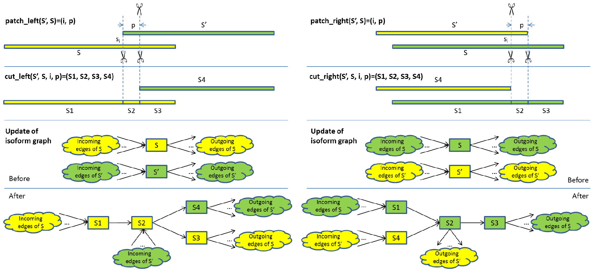
Given a set of sequences outputted by the seeding and growing algorithm (stage II), the patching and cutting algorithm (stage III) dynamically constructs an isoform graph. Initially, vertices in the graph are set as sequences from the input and the connection relationship (connected or not connected) between them is “unknown”. For every pair of vertices, the algorithm checks their connection relationship flag. If it is “unknown”, the two vertices are tested for patching. If patched, then their sequences are cut into segments, the vertices are split, directed edges are added, and the relationship flags between all involved vertices are updated accordingly. Sometimes this patching and cutting process may cause unnecessary cuts, i.e., it may generate some pairs of vertices connected only by one edge in the graph. If this happens, the two vertices are merged into one. After the isoform graph has been constructed, each linear path starting from a vertex with no incoming edges and ending at a vertex with no outgoing edge is put into an isoform structure set, and the joint sequence based on that path is put into a contigs set (Figure 3). Below is the mathematical description of the patching and cutting algorithm.

2.3.1 Definitions

Definition 7 (Patch).

Given two sequences $S=(s_{1}s_{2}...s_{l})$ and $S^{\prime}=(s^{\prime}_{1}s^{\prime}_{2}...s^{\prime}_{l^{\prime}})$ , $S^{\prime}$ is called a left patch of $S$ if we can find an $i$ and a $p\geq k$ for which $sub(S^{\prime},1,p)=sub(S,i,p)$ . We denote it as $patch\_left(S^{\prime},S)=(i,p)$ . Similarly, $S^{\prime}$ is called a right patch of $S$ if we can find an $i$ and a $p\geq k$ for which $sub(S^{\prime},l^{\prime}-p+1,p)=sub(S,i,p)$ . We denote it as $patch\_right(S^{\prime},S)=(i,p)$ .

Definition 8 (Cut).

Given two sequences $S=(s_{1}s_{2}...s_{l})$ and $S^{\prime}=(s^{\prime}_{1}s^{\prime}_{2}...s^{\prime}_{l^{\prime}})$ , if $patch\_left(S^{\prime},S)=(i,p)$ , a left cut between $S$ and $S^{\prime}$ splits them into four subsequences $(s_{1}s_{2}...s_{i-1})$ , $(s_{i}s_{i+1}...s_{i+p-1})$ , $(s_{i+p}s_{i+p+1}...s_{l})$ and $(s^{\prime}_{p+1}s^{\prime}_{p+2}...s^{\prime}_{l^{\prime}})$ . We denote this as $cut\_left(S^{\prime},S,i,p)=(S_{1},S_{2},S_{3},S_{4})$ . Similarly, if $patch\_right(S^{\prime},S)=(i,p)$ , a right cut between $S$ and $S^{\prime}$ splits them into four subsequences $(s_{1}s_{2}...s_{i-1})$ , $(s_{i}s_{i+1}...s_{i+p-1})$ , $(s_{i+p}s_{i+p+1}...s_{l})$ and $(s^{\prime}_{1}s^{\prime}_{2}...s^{\prime}_{l^{\prime}-p})$ . We denote this as $cut\_right(S^{\prime},S,i,p)=(S_{1},S_{2},S_{3},S_{4})$ .

Definition 9 (Joint).

Given two sequences $S=(s_{1}s_{2}...s_{l})$ and $S^{\prime}=(s^{\prime}_{1}s^{\prime}_{2}...s^{\prime}_{l^{\prime}})$ , a joint sequence between them is $(s_{1}s_{2}...s_{l}s^{\prime}_{1}s^{\prime}_{2}...s^{\prime}_{l^{\prime}})$ and is denoted as $joint(S,S^{\prime})$ . We also define the joint between $n$ sequences, $S_{1},S_{2},...,S_{n}$ as $joint(S_{1},S_{2},...,S_{n})=joint(S_{1},joint(S_{2},joint\\ (S_{3},...,joint(S_{n-1},S_{n}))))$ .

Definition 10 (Isoform graph, isoform structure and contig).

An isoform graph $G=(V,E)$ is a directed graph where each vertex is a sequence of letters from $\{A,T,C,G\}$ and each edge from vertex $V_{i}$ to vertex $V_{j}$ indicates that there exists a short read $R$ which is a subsequence of the joint sequence of $V_{i}$ and $V_{j}$ , i.e., $cover(R,joint(V_{i},V_{j}))=True$ . Given an isoform graph $G=(V,E)$ , an isoform structure is a linear path in $G$ starting at a vertex with no incoming edge and ending at a vertex with no outgoing edge. For an isoform structure with $n$ vertices as $V_{1}\rightarrow V_{2}\rightarrow...\rightarrow V_{n}$ , the corresponding contig is $joint(V_{1},V_{2},...,V_{n})$ .

2.3.2 A Patching and Cutting Algorithm

Algorithm Patching and Cutting

0: A set of sequences

S

and the minimum overlap length

k

0: An isoform graph

G=(V,E)

, a set of isoform structures

I

, and a set of contigs

C

V\leftarrow S

/* Initialize

V

, a set of vertices */

E\leftarrow\emptyset

/* Initialize

E

, a set of edges */

for each pair

V_{i},V_{j}\in V

F(V_{i},V_{j}),F(V_{j},V_{i})\leftarrow``unknown"

/* Initialize

F

, the relationship flags between vertices */

end for

for each pair

V_{i},V_{j}\in V

and

F(V_{i},V_{j})=``unknown"

patch\_left(V_{j},V_{i})=(v,p)

then

Update\_Graph(G,F,V_{i},V_{j},v,p,``left")

else if

patch\_right(V_{j},V_{i})=(v,p)

then

Update\_Graph(G,F,V_{i},V_{j},v,p,``right")

end if

end for

G\leftarrow Merge\_Vertices(G)

I\leftarrow Get\_Isoform\_Structures(G)

C\leftarrow\emptyset

/* Initialize

C

, a set of contigs */

for each isoform structure

I_{i}=V_{1}\rightarrow V_{2}\rightarrow...\rightarrow V_{n}\in I

C=C\cup\{joint(V_{1},V_{2},...,V_{n})\}

end for

Procedure Update_Graph $(G,F,V_{i},V_{j},v,p,dir)$

0: Isoform graph

G=(V,E)

, flags variable

F

, vertices

V_{i}

and

V_{j}

, cutting location variables

v

and

p

, and direction variable

dir

0: Updated graph

G

dir=``left"

then

(V_{1},V_{2},V_{3},V_{4})\leftarrow cut\_left(V_{j},V_{i},v,p)

else

(V_{1},V_{2},V_{3},V_{4})\leftarrow cut\_right(V_{j},V_{i},v,p)

end if

V\leftarrow(V-\{V_{i},V_{j}\})\cup\{V_{1},V_{2},V_{3},V_{4}\}

/* Remove two and add four vertices */

for each edge

V_{m}\rightarrow V_{n}\in E

V_{n}=V_{i}

then

replace

V_{n}

with

V_{1}

end if

V_{m}=V_{i}

then

replace

V_{m}

with

V_{3}

end if

V_{n}=V_{j}

then

dir=``left"

then

replace

V_{n}

with

V_{2}

else

replace

V_{n}

with

V_{4}

end if

V_{m}=V_{j}

then

dir=``left"

then

replace

V_{m}

with

V_{4}

else

replace

V_{m}

with

V_{2}

end if

end for

dir=``left"

then

E\leftarrow E\cup\{V_{1}\rightarrow V_{2},V_{2}\rightarrow V_{3},V_{2}\rightarrow V_{4}\}

/* Add three edges */

else

E\leftarrow E\cup\{V_{1}\rightarrow V_{2},V_{2}\rightarrow V_{3},V_{4}\rightarrow V_{2}\}

/* Add three edges */

end if

Update\_Flags(F,V_{i},V_{j},V_{1},V_{2},V_{3},V_{4})

Procedure Update_Flags $(F,V_{i},V_{j},V_{1},V_{2},V_{3},V_{4})$

0: Flags variable

F

and vertices

V_{i},V_{j},V_{1},V_{2},V_{3},V_{4}

0: Updated flags variable

F

delete flags

F(V_{i},V_{i})

and

F(V_{j},V_{j})

for each relationship flag

F(V_{m},V_{n})\in F

V_{m}=V_{i}

then

F(V_{1},V_{n}),F(V_{2},V_{n}),F(V_{3},V_{n})\leftarrow F(V_{m},V_{n})

F(V_{n},V_{1}),F(V_{n},V_{2}),F(V_{n},V_{3})\leftarrow F(V_{m},V_{n})

delete flags

F(V_{m},V_{n})

and

F(V_{n},V_{m})

end if

V_{m}=V_{j}

then

F(V_{2},V_{n}),F(V_{4},V_{n})\leftarrow F(V_{m},V_{n})

F(V_{n},V_{2}),F(V_{n},V_{4})\leftarrow F(V_{m},V_{n})

delete flags

F(V_{m},V_{n})

and

F(V_{n},V_{m})

end if

end for

for

1\leq m,n\leq 4

F(V_{m},V_{n})\leftarrow``known"

end for

F(V_{3},V_{4}),F(V_{4},V_{3})\leftarrow``unknown"

Procedure Merge_Vertices $(G)$

0: An isoform graph

G

0: Graph

G

with merged vertices

for each pair

V_{i},V_{j}\in V

V_{i}\rightarrow V_{j}\in E

is the only connection between them then

V_{m}\leftarrow joint(V_{i},V_{j})

/* Merge two vertices */

V\leftarrow(V-\{V_{i},V_{j}\})\cup\{V_{m}\}

/* Remove two vertices and add the merged vertex */

for each

V_{n}\rightarrow V_{i}\in E

Replace

V_{i}

with

V_{m}

/* Update incoming edges of

V_{i}

end for

for each

V_{j}\rightarrow V_{n}\in E

Replace

V_{j}

with

V_{m}

/* Update outgoing edges of

V_{j}

end for

end if

end for

Procedure Get_Isoform_Structures $(G)$

0: An isoform graph

G

0: An isoform structures set

I

I\leftarrow\emptyset

/* Initialize

I

for each vertex

V_{i}\in V

that has no incoming edge do

I\leftarrow\{V_{i}\}

end for

for each path

I_{i}=V_{i_{1}}\rightarrow V_{i_{2}}\rightarrow...\rightarrow V_{i_{n}}\in I

if vertex

V_{i_{n}}

has outgoing edges then

for each edge

V_{i_{n}}\rightarrow V_{i_{m}}\in E

I\leftarrow I\cup\{V_{i_{1}}\rightarrow V_{i_{2}}\rightarrow...\rightarrow V_{i_{n}}\rightarrow V_{i_{m}}\}

end for

I\leftarrow I-\{I_{i}\}

/* Remove

I_{i}

from

I

end if

end for

2.4 Error control

The above algorithms do not take into account the sequencing errors in short reads. In reality, due to those errors, the short reads do not always perfectly overlap with each other. Therefore the algorithms must have error tolerance capability in order to process real sequencing data. For this purpose, we slightly modify the following definitions:

Definition 11 (Overlap, updated).

A short read $P=(p_{1}p_{2}...p_{l})$ overlaps with $Q=(q_{1}q_{2}...q_{l})$ if $(p_{l-{l_{o}}+1}p_{l-{l_{o}}+2}...p_{l})=(q_{1}q_{2}...q_{l_{o}})$ for ${l_{o}}\geq k$ with at most $e_{1}l_{o}$ differences (errors) and no more than $e_{2}$ contiguous errors, where $l_{o}$ is the length of overlapped letters, $k$ is the minimum overlap cutoff, $e_{1}$ is the maximum error rate in any short read, i.e., there are at most $e_{1}*l$ sequencing errors in a short read of length $l$ . Here $e_{2}$ is a small constant, for instance, $2$ . Without loss of generality, we redefine the overlap between any two sequences in the same manner.

Definition 12 (Cover and Subsequence, updated).

Given two sequences $S=(s_{1}s_{2}...s_{l})$ and $S^{\prime}=(s^{\prime}_{1}s^{\prime}_{2}...s^{\prime}_{l^{\prime}})$ , $S^{\prime}$ is covered by $S$ if $l\geq l^{\prime}$ and $(s_{i+1}s_{i+2}...s_{i+l^{\prime}})=(s^{\prime}_{1}s^{\prime}_{2}...s^{\prime}_{l^{\prime}})$ for some $1\leq i\leq l$ with at most $e_{1}*l^{\prime}$ differences (errors) and no more than $e_{2}$ contiguous errors. We also say that $S^{\prime}$ is a subsequence of $S$ .

With these modified definitions, the proposed algorithms can be applied to process data with sequencing errors.

2.5 Complexity Analysis

2.5.1 The Localization and Binning Algorithm

Given a read aligner with running time $T(g,l)$ per short read, where $g$ is the length of the reference genome and $l$ is the short read length, the localization stage runs in $O(T(g,l)r)$ time, where $r$ is the total number of short reads. Running time of the binning step is $O(r\log r+r)=O(r\log r)$ because sorting genomic position takes $O(r\log r)$ time and the binning time after sorting is $O(r)$ . Therefore, the total time for localization and binning is $O(T(g,l)r+r\log r)$ . Since $T(g,l)$ is $\Omega(g)$ and $g\gg\log r$ , we have $O(T(g,l)r+r\log r)=O(T(g,l)r)$ , i.e., the time complexity of the localization and binning algorithm is mainly determined by the time complexity of the genome aligner.

2.5.2 The Seeding and Growing Algorithm

There are three major operations in this algorithm: $ext()$ , $merge()$ , and $cover()$ . Their time complexity depends on the basic $overlap()$ operation. For a short read with length $l$ , the time complexity of the $overlap()$ operation is $O(l)$ . Denoting the average number of short reads per bin as $m$ , in each extension, operation $ext()$ runs in $O(ml)$ time because there are $m$ pairs of short reads to test for overlaps. The time complexity of $merge()$ is $O(l)$ because the merging locations are already known from the preceding $ext()$ operation. The time complexity of $cover()$ is also $O(l)$ . Since the typical length of a grown sequence is $s$ and usually an $ext()$ operation extends a growing sequence by $O(l)$ letters, when seeding and growing a sequence, the number of times $ext()$ and $merge()$ operations are called is $O(\frac{s}{l})$ . The number of $cover()$ operations, when its input is limited to those overlapped short reads discovered by the $ext()$ operation, is only $O(\frac{s}{l}o)$ where $o$ is the number of overlapped short reads discovered when extending a read. Therefore, the total time for growing one sequence is $O(\frac{s}{l}ml)+O(\frac{s}{l}l)+O(\frac{s}{l}ol)$ = $O(sm)$ as $m>o$ . Also, there are only a small number of such sequences to grow. Typically this number is $O(1)$ . Thus the total time for growing all the sequences in one bin or transcriptional unit is $O(sm)$ . The total time for growing all the sequences in $n$ bin or transcriptional units in a whole transcriptome is $O(smn)=O(sr)$ where r is the total number of short reads. Typical values of $s$ and $r$ are $O(10^{3})$ and $O(10^{7})\sim O(10^{8})$ , respectively.

2.5.3 The Patching and Cutting Algorithm

The time complexity of the patching and cutting algorithm is determined by the number of vertices and the number of edges in the isoform graph. Because there are only $O(1)$ sequences generated in the seeding and growing stage, typically the number of vertices in the final graph is $O(1)\sim O(10)$ and the number of edges is $O(1)\sim O(10^{2})$ at most. As these numbers are much smaller than $s$ , $m$ , and $n$ , the time complexity of the patching and cutting algorithm can be neglected.

The total time complexity of the algorithms for short reads localization, transcriptome assembly and isoforms reconstruction is thus $O(T(g,l)r+sr)$ . Since $T(g,l)$ is $\Omega(g)$ and $g\gg s$ , the complexity is mainly determined by the read mapping algorithm.

3 Simulation Experiments

We used FluxSimulator [http://flux.sammeth.net], an open source software package simulating whole transcriptome sequencing experiments, to generate RNA-Seq data sets. FluxSimulator first randomly generates integer copies of each splicing isoform according to the user-provided annotation file. It then constructs an amplified, size-selected library and sequences the library in silico. The resulting cDNA fragments are then sampled randomly for simulated sequencing, where the initial and terminal ends of each selected fragment are reported as reads. The current version of FluxSimulator (1.2) provides two sequencing error models, one is for read length $76$ and another is for read length $36$ . The default error model was used to generate six data sets consisting of $15$ million, $20$ million, $30$ million, $50$ million, $75$ million, and $100$ million paired-end reads with length $76$ from the reference protein-coding transcripts available from the Ensembl database (version GRCh37.69). More details of the simulated data sets and the error model can be found in the Appendix. Both simulated RNA-Seq data sets and implementation of SPATA are available for download at http://sammate.sourceforge.net/.

We compared the performance of SPATA with Cufflinks [19] and Trinity [41]. Cufflinks is a reference-guided transcriptome assembly whereas Trinity is a de novo transcriptome assembly [15, 16]. As mentioned before, SPATA is a hybridization of the reference-guided and the de novo strategies, i.e., it uses the reference genome to localize reads to genomic loci and then assembles the read sequences falling into each genomic locus using a new assembly algorithm. Simulated FASTQ files were used as input for SPATA and Trinity. Since Cufflinks does not process raw reads, we used TopHat [23] to align reads from the FASTQ files to the human reference genome. We then used TopHat’s BAM files as the input for Cufflinks. We used default parameters to run all the tools.

3.1 Precision and Accuracy Analyses

For each dataset, the ground truth is a set of expressed transcript sequences whereas the output of each assembly software is a set of contigs, i.e., a continuous sequence of bases constructed from the short reads in the FASTQ files. In the rest of the manuscript, we use the term reference transcripts to refer to the expressed transcript sequences. Output contigs of each assembly program were compared against the reference transcripts using the pairwise sequence alignment program SSAHA2 [45]. We evaluated and compared the performance of the assembly programs according to “precision” and “accuracy”. When output contigs were aligned to the reference transcripts, we define the precision as the fraction of contigs that were properly mapped to the reference transcripts. A contig is considered to be mapped if at least $90\%$ of its sequence was covered by a reference transcript ( $\frac{M}{M+N+G}\geq 90\%$ , where $M$ is the number of matched bases, $N$ is the number of mismatched bases and $G$ is the cumulative insertion and deletion length). When the reference transcripts were aligned to the constructed contigs, we define the accuracy as the fraction of reference transcripts that can be fully reconstructed. A transcript is defined to be fully reconstructed if it has at least $90\%$ base-identity with one of the output contigs.

When evaluating the performance of different assembly software, high values for both precision and accuracy are important. On one hand, a high precision indicates that most of the method’s contigs are subsequences of the reference transcripts. On the other hand, a high accuracy indicates that a method reconstructed a large number of the reference transcripts.

Regarding precision, we calculated the fraction of output contigs of Cufflinks, Trinity, and SPATA that were properly mapped to the reference transcripts. Figure 4 displays the fraction of contigs that were mapped to reference transcripts. The performance comparison in terms of precision is overall comparable with slightly higher values for Cufflinks. It might due to the following reasons: First, Cufflinks only processes reads that were aligned to the reference genome and discards reads with sequencing errors. Second, Cufflinks attempts to identify the minimum number of isoforms that cover the majority of reads.

Regarding accuracy, we calculated the fraction of reference transcripts that can be fully reconstructed by Cufflinks, Trinity, and SPATA. Figure 5 displays the number of reference transcripts that were fully reconstructed across a broad ranges of expression levels and sequencing depths. The expression of the reference transcripts is calculated from the simulated ground truth origin of the paired-end reads, i.e., the mean coverage of a transcript is calculated as the number of reads multiplied with the read length divided by the transcript length. We examined all reference transcripts having mean coverage of $5$ or higher.

In general, Cufflinks performed better at low expression levels whereas SPATA and Trinity performed better at high expression levels (Figure 5). Cufflinks may perform better at lower expression levels since the small gaps within a transcript caused by sequencing errors or lack of read coverage can be corrected using the reference genome [19, 15, 16]. Trinity and SPATA, however, outperform Cufflinks in assembling highly reference transcripts. A possible reason is that the parsimony strategy used by Cufflinks attempts to identify the minimum number of isoforms to cover the majority of reads while filtering out uncertain reads. The latter may result in missing some alternative splicing events [19, 15, 16, 22].

Another notable phenomenon is that SPATA reconstructs more reference transcripts than Cufflinks and Trinity for any of the six data sets. Figure 6 displays the total number of reference transcripts reconstructed by each method across all of the six data sets. Interestingly, Trinity and SPATA reconstruct more reference transcripts as the number of reads increases whereas the number of reference transcripts reconstructed by Cufflinks fluctuates.

3.2 Robust Analysis Using Incomplete Reference Genomes

In the above analyses, Cufflinks and SPATA used the human reference genome version GRCh37.69 downloaded from Ensembl. The same genome sequence was used to generate the simulated data sets by FluxSimulator. We consider this latest version of human genome as the “complete” reference genome. In order to access the robustness of Cufflinks and SPATA against incomplete reference genomes, we also examined their performance using different versions of the human reference genome. We downloaded the following reference genome sequences from UCSC website: hg10 (December 2001), hg12 (June 2002), hg15 (April 2004), hg17 (February 2009), and hg19 (October 2012). The older a reference genome, the more incomplete it is compared to the complete reference genome (Ensembl GRCh37.69).

Figure 7 displays the precision and accuracy of Cufflinks, Trinity, and SPATA for the data set consisting of $15$ million reads. Since Trinity did not use any reference genome, its constant performance was used as a benchmark to compare the performance of Cufflinks and SPATA. In Figure 7, the left panel displays the precision of the assembly tools whereas the right panel displays their accuracy. The number of reference transcripts reconstructed by Cufflinks, Trinity, and SPATA is displayed in Figure 8 in the Appendix.

In terms of precision, the performance of Cufflinks and SPATA are comparable and are consistently higher than that of Trinity. This translates into a robust precision of Cufflinks and SPATA, regardless of quality of the reference genome being used. In terms of accuracy, as the quality of the reference genome declines, the performance of Cufflinks and SPATA also declines and a sharper drop is observed for Cufflinks. For the reference genome sequence hg10, a low-quality reference genome, the accuracy of Trinity and SPATA is almost the same and is higher than that of Cufflinks. For all other reference genome sequences, SPATA achieves a better accuracy than Cufflinks and Trinity.

4 Conclusion

In this paper, we presented SPATA, a hybrid transcriptome assembly approach, to reconstruct transcriptomes via a novel three-stage algorithm: localization, seeding and growing, and patching and cutting. We first assessed the performance of SPATA by reconstructing the transcritomes using multiple simulated RNA-Seq data sets for which SPATA achieves high precision and accuracy. We also showed that SPATA reconstructs more reference transcripts than the selected transcriptome assembly tools for all of the simulated data sets. We further demonstrated the robustness of SPATA against incomplete reference genomes by using different versions of human reference genome over the past $12$ years. SPATA consistently achieved a high precision and reconstructed more reference transcripts than the competing methods. Overall, the analyses favor the use of SPATA in transcriptome reconstruction wherever a reference genome is available, regardless of quality.

SPATA is also expected to be a valuable tool to assemble transcriptomes of non-model organisms, where the reference genome sequences are likely to be incomplete. Despite advances in sequencing technologies, assembling a complete reference genome is still costly and difficult for many species. As a result, most of the existing genomes are available only as unfinished drafts with gaps and excessive assembly errors [46, 47, 48]. In these cases, SPATA is expected to reliably capture both known transcript structures and novel variations due to its high precision and accuracy. SPATA is also conveniently accessible for both informatics and life science researchers via an easy-to-use GUI software.

5 Appendix

Figure 8 displays the number of reference transcripts that were fully reconstructed by Cufflinks, Trinity, and SPATA using different reference genomes for the data set consisting of $15$ million reads. Since the total number of reference transcripts is a constant, the number of the reference transcripts reconstructed by the assembly tools also reflects their accuracy. For the low-quality reference genome genome hg10, SPATA and Trinity reconstruct almost the same number of reference transcripts and reconstruct more than Cufflinks. For all other reference genome sequences, SPATA reconstructs more reference transcripts than Cufflinks and Trinity.

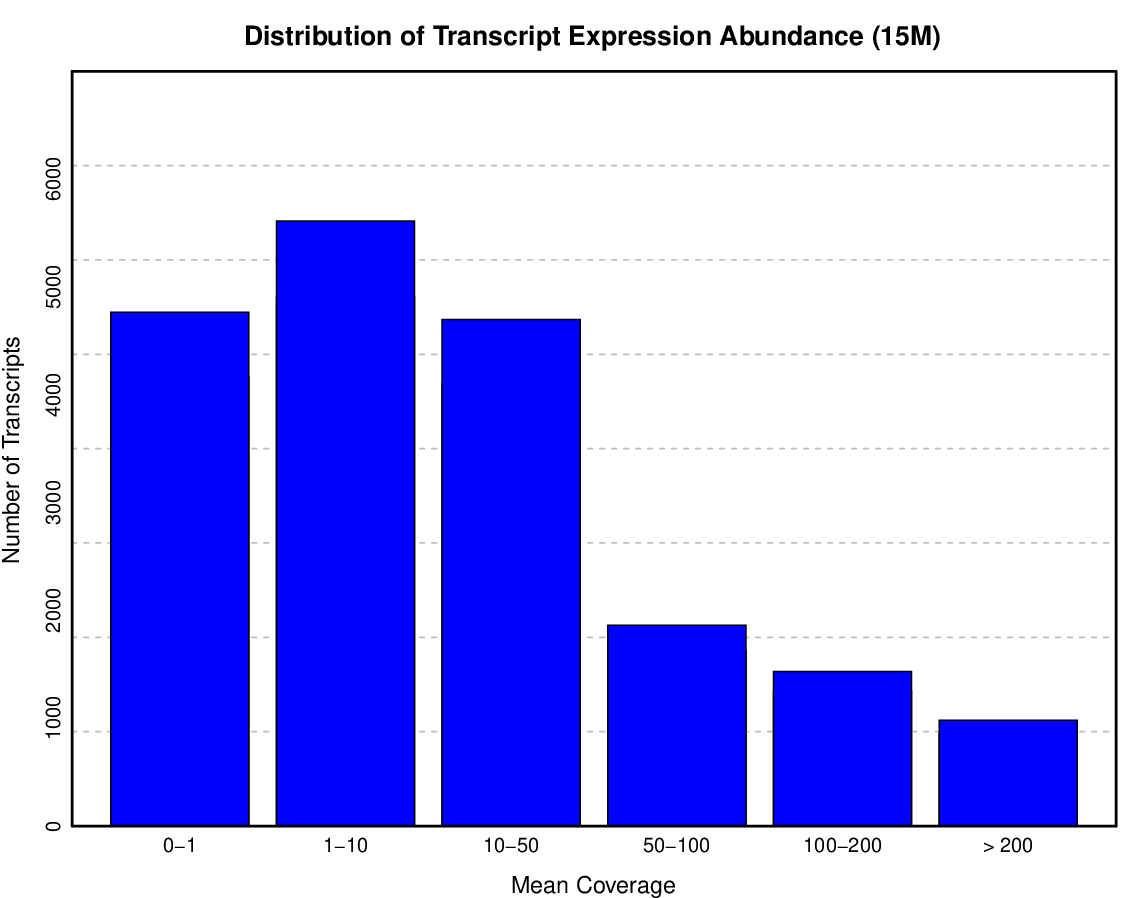
The statistics of the simulated data are displayed in Table 1, Figure 9 and Figure 10. Table 1 shows the number of reference transcripts in each data set. Figure 9 displays the quality score distribution of sequenced bases across $76$ read positions whereas Figure 9 displays the expression abundance distribution of the reference transcripts.

Table 1: Number of reference transcripts

Data sets	Expressed transcripts	Transcripts having
		coverage $\geq 5$
15M	19,351	10,784
20M	19,390	11,357
30M	19,299	12,326
50M	19,316	13,360
75M	19,380	14,424
100M	19,344	15,160

References

[1] Matlin, A. J., Clark, F. and Smith, C. W. J. (2005) Understanding alternative splicing: towards a cellular code. Nature Reviews Molecular Cell Biology, 6(5), 386 – 398.
[2] Mortazavi, A., Williams, B. A., McCue, K., Schaeffer, L. and Wold, B. (2008) Mapping and quantifying mammalian transcriptomes by RNA-Seq. Nature Methods, 5(7), 621–628.
[3] Wang, E. T., Sandberg, R., Luo, S., Khrebtukova, I., Zhang, L., Mayr, C., Kingsmore, S. F., Schroth, G. P. and Burge, C. B. (2008) Alternative isoform regulation in human tissue transcriptomes. Nature, 456(7221), 470–476.
[4] Maher, C. A., Kumar-Sinha, C., Cao, X., Kalyana-Sundaram, S., Han, B., Jing, X., Sam, L., Barrette, T., Palanisamy, N. and Chinnaiyan, A. M. (2009) Transcriptome sequencing to detect gene fusions in cancer. Nature, 458(7234), 97 – 101.
[5] Medvedev, P., Stanciu, M. and Brudno, M. (2009) Computational methods for discovering structural variation with next-generation sequencing. Nature Methods, 6(11 Suppl), S13–S20.
[6] Medvedev, P., Fiume, M., Dzamba, M., Smith, T. and Brudno, M. (2010) Detecting copy number variation with mated short reads. Genome Research, 20(11), 1613–1622.
[7] Wang, X.-S., Prensner, J. R., Chen, G., Cao, Q., Han, B., Dhanasekaran, S. M., Ponnala, R., Cao, X., Varambally, S., Thomas, D. G. et al. (2009) An integrative approach to reveal driver gene fusions from paired-end sequencing data in cancer. Nature Biotechnology, 27(11), 1005–1011.
[8] Barash, Y., Calarco, J. A., Weijun, G., Qun, P., Xinchen, W., Shai, O., Blencowe, B. J. and Frey, B. J. (2010) Deciphering the splicing code. Nature, 465(7294), 53 – 59.
[9] Nguyen, T. C., Deng, N. and Zhu, D. (2012) SASeq: A Selective and Adaptive Shrinkage Approach to Detect and Quantify Active Transcripts using RNA-Seq. arXiv preprint arXiv:1208.3619,.
[10] Feuk, L., Carson, A. R. and Scherer, S. W. (2006) Structural variation in the human genome. Nature Reviews Genetics, 7(2), 85–97.
[11] Pan, Q., Shai, O., Lee, L. J., Frey, B. J. and Blencowe, B. J. (2008) Deep surveying of alternative splicing complexity in the human transcriptome by high-throughput sequencing. Nature genetics, 40(12), 1413–1415.
[12] Croft, L., Schandorff, S., Clark, F., Burrage, K., Arctander, P. and Mattick, J. S. (2000) ISIS, the intron information system, reveals the high frequency of alternative splicing in the human genome.. Nat Genet, 24(4), 340–341.
[13] Ozsolak, F. and Milos, P. M. (2010) RNA sequencing: advances, challenges and opportunities. Nature Reviews Genetics, 12(2), 87–98.
[14] Haas, B. J., Zody, M. C. et al. (2010) Advancing RNA-seq analysis. Nature biotechnology, 28(5), 421.
[15] Martin, J. A. and Wang, Z. (2011) Next-generation transcriptome assembly. Nature Reviews Genetics,.
[16] Garber, M., Grabherr, M. G., Guttman, M. and Trapnell, C. (2011) Computational methods for transcriptome annotation and quantification using RNA-Seq. Nature methods, 8(6), 469–477.
[17] Denoeud, F., Aury, J.-M., Da Silva, C., Noel, B., Rogier, O., Delledonne, M., Morgante, M., Valle, G., Wincker, P., Scarpelli, C. et al. (2008) Annotating genomes with massive-scale RNA sequencing. Genome Biology, 9(12), R175.
[18] Guttman, M., Garber, M., Levin, J. Z., Donaghey, J., Robinson, J., Adiconis, X., Fan, L., Koziol, M. J., Gnirke, A., Nusbaum, C. et al. (2010) Ab initio reconstruction of cell type-specific transcriptomes in mouse reveals the conserved multi-exonic structure of lincRNAs. Nature Biotechnology, 28(5), 503–510.
[19] Trapnell, C., Williams, B. A., Pertea, G., Mortazavi, A., Kwan, G., van Baren, M. J., Salzberg, S. L., Wold, B. J. and Pachter, L. (2010) Transcript assembly and quantification by RNA-Seq reveals unannotated transcripts and isoform switching during cell differentiation. Nature Biotechnology, 28(5), 511 – 515.
[20] Feng, J., Li, W. and Jiang, T. (2011) Inference of isoforms from short sequence reads. Journal of computational biology, 18(3), 305–321.
[21] Li, W. and Jiang, T. (2012) Transcriptome assembly and isoform expression level estimation from biased RNA-Seq reads. Bioinformatics, 28(22), 2914–2921.
[22] Li, W., Feng, J. and Jiang, T. (2011) IsoLasso: A LASSO Regression Approach to RNA-Seq Based Transcriptome Assembly. Journal of Computational Biology, 18(11), 1693–1707.
[23] Trapnell, C., Pachter, L. and Salzberg, S. L. (2009) TopHat: discovering splice junctions with RNA-Seq. Bioinformatics, 25(9), 1105–1111.
[24] Ameur, A., Wetterbom, A., Feuk, L. and Gyllensten, U. (2010) Global and unbiased detection of splice junctions from RNA-seq data. Genome Biology, 11(3), R34+.
[25] Wang, K., Singh, D., Zeng, Z., Coleman, S. J., Huang, Y., Savich, G. L., He, X., Mieczkowski, P., Grimm, S. A., Perou, C. M. et al. (2010) MapSplice: Accurate mapping of RNA-Seq reads for splice junction discovery. Nucleic Acids Research,.
[26] Dimon, M. T., Sorber, K. and DeRisi, J. L. (2010) MMSplicer: A Tool for Efficient and Sensitive Discovery of Known and Novel Splice Junctions in RNA-Seq Data. PLoS ONE, 5(11), e13875.
[27] Au, K. F., Jiang, H., Lin, L., Xing, Y. and Wong, W. H. (2010) Detection of splice junctions from paired-end RNA-seq data by SpliceMap. Nucleic Acids Research,.
[28] Lou, S.-K., Ni, B., Lo, L.-Y., Tsui, S. K.-W., Chan, T.-F. and Leung, K.-S. (2011) ABMapper: a suffix array-based tool for multi-location searching and splice-junction mapping. Bioinformatics, 27(3), 421–422.
[29] Kinsella, M., Harismendy, O., Nakano, M., Frazer, K. and Bafna, V. (2011) Sensitive gene fusion detection using ambiguously mapping RNA-Seq read pairs. Bioinformatics, 27(8), 1068–1075.
[30] de Bruijn, N. G. and Erdos, P. (1946) A combinatorial problem. Koninklijke Netherlands: Academe Van Wetenschappen, 49, 758–764.
[31] Good, I. J. (1946) Normal recurring decimals. Journal of the London Mathematical Society, 1(3), 167.
[32] Pevzner, P. A., Tang, H. and Waterman, M. S. (2001) An Eulerian path approach to DNA fragment assembly. Proceedings of the National Academy of Sciences, 98(17), 9748–9753.
[33] Zerbino, D. R. and Birney, E. (2008) Velvet: algorithms for de novo short read assembly using de Bruijn graphs. Genome research, 18(5), 821–829.
[34] Butler, J., MacCallum, I., Kleber, M., Shlyakhter, I. A., Belmonte, M. K., Lander, E. S., Nusbaum, C. and Jaffe, D. B. (2008) ALLPATHS: De novo assembly of whole-genome shotgun microreads. Genome research, 18(5), 810–820.
[35] Simpson, J. T., Wong, K., Jackman, S. D., Schein, J. E., Jones, S. J. and Birol, n. (2009) ABySS: A parallel assembler for short read sequence data. Genome Research, 19(6), 1117–1123.
[36] Pell, J., Hintze, A., Canino-Koning, R., Howe, A., Tiedje, J. M. and Brown, C. T. (2012) Scaling metagenome sequence assembly with probabilistic de Bruijn graphs. Proceedings of the National Academy of Sciences, 109(33), 13272–13277.
[37] Martin, J., Bruno, V. M., Fang, Z., Meng, X., Blow, M., Zhang, T., Sherlock, G., Snyder, M. and Wang, Z. (2010) Rnnotator: an automated de novo transcriptome assembly pipeline from stranded RNA-Seq reads. BMC genomics, 11(1), 663.
[38] Birol, I., Jackman, S. D., Nielsen, C. B., Qian, J. Q., Varhol, R., Stazyk, G., Morin, R. D., Zhao, Y., Hirst, M., Schein, J. E. et al. (2009) De novo transcriptome assembly with ABySS. Bioinformatics, 25(21), 2872–2877.
[39] Robertson, G., Schein, J., Chiu, R., Corbett, R., Field, M., Jackman, S. D., Mungall, K., Lee, S., Okada, H. M. M., Qian, J. Q. et al. (2010) De novo assembly and analysis of RNA-Seq data. Nature Methods, 7(11), 909–912.
[40] Surget-Groba, Y. and Montoya-Burgos, J. I. (2010) Optimization of de novo transcriptome assembly from next-generation sequencing data. Genome Research, 20(10), 1432–1440.
[41] Grabherr, M. G., Haas, B. J., Yassour, M., Levin, J. Z., Thompson, D. A., Amit, I., Adiconis, X., Fan, L., Raychowdhury, R., Zeng, Q. et al. (2011) Full-length transcriptome assembly from RNA-Seq data without a reference genome. Nature Biotechnology, 29(7), 644–652.
[42] Schulz, M. H., Zerbino, D. R., Vingron, M. and Birney, E. (2012) Oases: robust de novo RNA-Seq assembly across the dynamic range of expression levels. Bioinformatics, 28(8), 1086–1092.
[43] Langmead, B., Trapnell, C., Pop, M., Salzberg, S. L. et al. (2009) Ultrafast and memory-efficient alignment of short DNA sequences to the human genome. Genome Biology, 10(3), R25.
[44] Langmead, B. and Salzberg, S. L. (2012) Fast gapped-read alignment with Bowtie 2. Nature Methods, 9(4), 357–359.
[45] Ning, Z., Cox, A. J. and Mullikin, J. C. (2001) SSAHA: a fast search method for large DNA databases.. Genome research, 11(10), 1725–1729.
[46] Salzberg, S. L. and Yorke, J. (2005) Beware of mis-assembled genomes. Bioinformatics (Oxford, England), 21(24).
[47] Salzberg, S. L., Phillippy, A. M., Zimin, A., Puiu, D., Magoc, T., Koren, S., Treangen, T. J., Schatz, M. C., Delcher, A. L., Roberts, M. et al. (2012) GAGE: A critical evaluation of genome assemblies and assembly algorithms. Genome research, 22(3), 557–567.
[48] Baker, M. (2012) De novo genome assembly: what every biologist should know. Nature methods, 9(4), 333–337.