The Brownian Mean Field model

Pierre-Henri Chavanis E-mail: chavanis@irsamc.ups-tlse.fr Affiliation: Laboratoire de Physique Théorique (IRSAMC), CNRS and UPS, Université de Toulouse, F-31062 Toulouse, France

To be included later

Abstract

We discuss the dynamics and thermodynamics of the Brownian Mean Field (BMF) model which is a system of $N$ Brownian particles moving on a circle and interacting via a cosine potential. It can be viewed as the canonical version of the Hamiltonian Mean Field (HMF) model. The BMF model displays a second order phase transition between a homogeneous phase and an inhomogeneous phase below a critical temperature $T_{c}=1/2$ . We first complete the description of this model in the mean field approximation valid for $N\rightarrow+\infty$ . In the strong friction limit, the evolution of the density towards the mean field Boltzmann distribution is governed by the mean field Smoluchowski equation. For $T<T_{c}$ , this equation describes a process of self-organization from a non-magnetized (homogeneous) phase to a magnetized (inhomogeneous) phase. We obtain an analytical expression for the temporal evolution of the magnetization close to $T_{c}$ . Then, we take fluctuations (finite $N$ effects) into account. The evolution of the density is governed by the stochastic Smoluchowski equation. From this equation, we derive a stochastic equation for the magnetization and study its properties both in the homogenous and inhomogeneous phases. We show that the fluctuations diverge close to the critical point so that the mean field approximation ceases to be valid. Actually, the limits $N\rightarrow+\infty$ and $T\rightarrow T_{c}$ do not commute. The validity of the mean field approximation requires $N(T-T_{c})\rightarrow+\infty$ so that $N$ must be larger and larger as $T$ approaches $T_{c}$ . We show that the direction of the magnetization changes rapidly close to $T_{c}$ but its amplitude takes a long time to relax. We also indicate that, for systems with long-range interactions, the lifetime of metastable states scales as $e^{N}$ except close to a critical point. The BMF model shares many analogies with other systems of Brownian particles with long range interactions such as self-gravitating Brownian particles, the Keller-Segel model describing the chemotaxis of bacterial populations, and the Kuramoto model describing the collective synchronization of coupled oscillators.

pacs

05.20.-y Classical statistical mechanics - 05.45.-a Nonlinear dynamics and chaos - 05.20.Dd Kinetic theory - 64.60.De Statistical mechanics of model systems

1 Introduction

In the recent years, the statistical mechanics of systems with long-range interactions has been a topic of active research [1, 2, 3, 4]. In most papers devoted to this subject, one assumes that the system is isolated. This corresponds to the microcanonical ensemble in which the energy is conserved. This is the proper description of self-gravitating systems such as galaxies and globular clusters in astrophysics. Indeed, they can be viewed as isolated Hamiltonian systems of $N$ point mass stars in gravitational interaction described by the Newton equations [5]. This is also the correct approach to the point vortex gas in 2D hydrodynamics described by the Kirchhoff equations [6]. Actually, the statistical mechanics of stellar systems and two-dimensional vortices share many analogies [7]. Systems with long-range interactions display very interesting properties such as ensemble inequivalence, negative specific heats, spatially inhomogeneous equilibrium states, violent collisionless relaxation, slow collisional relaxation, non-Boltzmannian quasistationary states (QSS) etc. The dynamics and thermodynamics of these systems is now relatively well-understood [4] even if some conceptual issues remain such as the precise nature of the QSSs.

However, in many situations of physical interest, the system is not isolated from the surrounding and it is important to take into account its interaction with the external medium. This interaction usually results in some effects of forcing and dissipation. In the simplest situation, the one that we shall consider here, the forcing and the dissipation satisfy a detailed balance condition so that, formally, the system can be thought to be in contact with a thermal bath fixing its temperature $T$ . We stress that the thermostat is played by a system of another nature (physically different from the system under consideration) which usually has short-range interactions¹¹ 1 Indeed, it is not possible to define the notion of thermostat for a purely long-range system (i.e. to divide the system into a subsystem $+$ a reservoir) since the energy is non-additive [4].. To be specific, let us consider a particular example issued from astrophysics. In the context of planet formation, one has to study the motion of dust particles in gravitational interaction evolving in a gas (the solar nebula) [8]. In addition to the long-range gravitational interaction, the dust particles experience a friction with the gas and a stochastic force (noise) due to turbulence or Brownian motion (i.e. short-range collisions with the molecules of the gas). This situation can be described by $N$ stochastic Langevin equations, one for each particle, coupled together by the gravitational interaction. This defines the self-gravitating Brownian model. If we assume a detailed balance condition, the diffusion coefficient $D$ and the friction coefficient $\xi$ satisfy the Einstein relation $D=\xi k_{B}T/m$ where $T$ is the temperature of the bath. In that case, the proper statistical ensemble is the canonical ensemble. The self-gravitating Brownian model has been studied in a series of papers by Chavanis and Sire (see, e.g., [9] and references therein) in the strong friction limit $\xi\rightarrow+\infty$ in which the motion of the particles is overdamped. Some interesting analogies with the chemotaxis of bacterial populations, the so-called Keller-Segel model [10], have been developed in these papers. Indeed, bacterial populations may be considered as a system of Brownian particles with long-range interactions. The bacteria have a diffusive motion (due to their flagella) but they also secrete a substance (a sort of pheromone) and are collectively attracted by this substance. Interestingly, it can be shown that the concentration of the secreted chemical plays the same role as the gravitational potential. This long-range attraction may result in chemotactic collapse. As a result, the Smoluchowski-Poisson system and the Keller-Segel models are isomorphic [11]. Furthermore, in biology, the overdamped limit is justified because inertial effects are generally negligible.

In order to study systems with long-range interactions in a simple setting, toy models have been introduced in statistical mechanics. In particular, the Hamiltonian Mean Field (HMF) model has received a particular attention [12-37]. This model consists in $N$ particles of unit mass moving on a circle and interacting via a cosine potential $u=N^{-1}[1-\cos(\theta_{i}-\theta_{j})]$ where $\theta_{i}$ denotes the angle that particle $i$ makes with an axis of reference. Since the energy is conserved, the fundamental statistical description of the HMF model is the microcanonical ensemble. It can be of interest to consider in parallel the case of a system in which the particles experience, in addition to the cosine interaction, a friction force and a stochastic force. In that case, their dynamics is described by coupled Langevin equations. Like for the model of self-gravitating Brownian particles, we assume that a detailed balance condition holds. We thus consider a system of Brownian particles with cosine interaction in contact with a thermal bath. This is the so-called Brownian Mean Field (BMF) model [17, 38]. Since the temperature is fixed, the fundamental statistical description of the BMF model is the canonical ensemble. It has been demonstrated in [39] that Hamiltonian reservoirs microscopically coupled with the system [40, 41] and Langevin thermostats [17] provide equivalent descriptions even out-of-equilibrium. Therefore, the BMF model has many applications. It is also connected to the Kuramoto model [42] describing the collective synchronization in spatially extended systems of coupled oscillators²² 2 The Kuramoto model is, however, more complicated since the oscillators usually have different frequencies. A generalization of the BMF model, called the $\alpha$ -BMF model, has been considered recently [43].

The Brownian Mean Field model was introduced and studied in [17]. However, in this work, the effect of fluctuations was neglected and a mean field approximation was considered. For systems with long-range interactions the mean field approximation is usually exact in the thermodynamic limit $N\rightarrow+\infty$ . However, this is no longer true in the vicinity of a critical point. In that case, the limits $N\rightarrow+\infty$ and $T\rightarrow T_{c}$ do not commute and the effect of fluctuations must be properly taken into account. The objective of the present paper is to go beyond the mean field approximation considered in [17] and study the effect of fluctuations. We shall be particularly interested in the behavior of the magnetization close to the critical point. We show that it is described by the usual phenomenology of second order phase transitions. However, an interest of the BMF model is that we can derive the stochastic equation for the magnetization ${\bf M}(t)$ directly from the $N$ -body dynamics by using the stochastic Smoluchowski equation. As a result, the number of particles $N$ explicitly enters in the equations and leads to novel effects such as the non-commutation of the limits $N\rightarrow+\infty$ and $T\rightarrow T_{c}$ , and the fact that the metastable states have very long lifetimes scaling as $e^{N}$ (except close to a critical point).

The paper is organized as follows. In Section 2 we introduce the BMF model and present the basic equations. In Section 3, to simplify the study, we consider the strong friction limit $\xi\rightarrow+\infty$ in which the inertia of the particles can be neglected. In Section 4, we determine the statistical equilibrium state of the BMF model in the canonical ensemble. It displays a second order phase transition at the critical temperature $T_{c}=1/2$ . We solve the thermodynamical stability problem by different methods and study the equilibrium fluctuations of the magnetization. We show that they diverge at the critical point. We also investigate the effect of an external magnetic field and show that the magnetic susceptibility also diverges at the critical point. In Section 5, we study the dynamical stability of a steady state of the mean field Smoluchowski equation and show the equivalence between dynamical and thermodynamical stability. In Section 6, we apply the linear response theory to the BMF model and study the response of the system to an external perturbation such as a pulse or a step function. In Section 7, we study the evolution of the mean magnetization in the inhomogeneous phase and solve the equations perturbatively close to the critical point. We obtain an analytical expression for the temporal evolution of the magnetization close to $T_{c}$ . In Section 8, we study the temporal correlations of the magnetization in the homogeneous phase. We show that they diverge as we approach the critical point implying that the mean field approximation ceases to be valid close to the critical point and that the instability occurs sooner than predicted by the linear stability analysis. We also explicitly check in this particular situation the fluctuation-dissipation theorem. In Section 9 we study the fluctuations of the magnetization in the homogeneous phase and show that they can be described by an Ornstein-Uhlenbeck process. The evolution of the probability density of the magnetization is described by a linear Fokker-Planck equation analogous to the Kramers equation. Finally, in Section 10, we study the fluctuations of the magnetization in the inhomogeneous phase and solve the problem perturbatively close to the critical point. As $T\rightarrow T_{c}$ , we show that the direction of the magnetization changes rapidly while its magnitude takes a long time to relax towards its equilibrium value.

2 The inertial BMF model

2.1 The Langevin equations

The BMF model is a system of $N$ Brownian particles of unit mass moving on a circle and interacting via a cosine binary potential [17]. The dynamics of these particles is governed by the coupled stochastic Langevin equations

	$\displaystyle{d\theta_{i}\over dt}=v_{i},\qquad\qquad\qquad\qquad\qquad\qquad\qquad\quad$
	$\displaystyle{dv_{i}\over dt}=-{\partial\over\partial\theta_{i}}U(\theta_{1},...,\theta_{N})-\xi v_{i}+\sqrt{2D}R_{i}(t),$		(1)

where $i=1,...,N$ label the particles. The particles interact through the potential $U(\theta_{1},...,\theta_{N})=\frac{1}{N}\sum_{i<j}u(\theta_{i}-\theta_{j})$ where

u(\theta-\theta^{\prime})=1-\cos(\theta-\theta^{\prime}),

(2)

is the cosine potential. This potential is attractive and the particles tend to group themselves in order to decrease their potential energy. This tendency is of course counter-balanced by thermal motion. The Hamiltonian is $H=\sum_{i=1}^{N}{v_{i}^{2}\over 2}+U(\theta_{1},...,\theta_{N})$ . We have rescaled the potential energy by $1/N$ to make the system extensive. This corresponds to the Kac prescription [44]. We note, however, that the energy remains fundamentally non-additive [4]. $R_{i}(t)$ is a Gaussian white noise satisfying $\langle R_{i}(t)\rangle=0$ and $\langle R_{i}(t)R_{j}(t^{\prime})\rangle=\delta_{ij}\delta(t-t^{\prime})$ . $D$ and $\xi$ are respectively the diffusion and friction coefficients. The former measures the strength of the noise, whereas the latter quantifies the dissipation to the external environment. We assume that these two effects have the same physical origin, like when the system interacts with a heat bath. In particular, we suppose that the temperature $T$ of the bath satisfies the Einstein relation $D=\xi T$ . The temperature measures the strength of the stochastic force for a given friction coefficient. For $\xi=D=0$ , we recover the HMF model [12] which conserves the energy $H$ .

To monitor the evolution of the system, it is convenient to introduce the magnetization ${\bf M}=(M_{x},M_{y})$ with components

\displaystyle M_{x}=\frac{1}{N}\sum_{i=1}^{N}\cos\theta_{i},\qquad M_{y}=\frac{1}{N}\sum_{i=1}^{N}\sin\theta_{i}.

(3)

The magnetization can serve as an order parameter in the BMF model. In terms of the magnetization, the potential energy is exactly given by $U=N(1-M^{2})/2$ . The force acting on particle $i$ is $F_{i}=-{\partial U\over\partial\theta_{i}}$ . Using Eqs. (2) and (3) it can be written as $F_{i}=-\frac{1}{N}\sum_{j}\sin(\theta_{i}-\theta_{j})=-M_{x}\sin\theta_{i}+M_{y}\cos\theta_{i}$ .

2.2 The $N$ -body Kramers equation

The evolution of the $N$ -body distribution function is governed by the Fokker-Planck equation [45]:

	$\displaystyle{\partial P_{N}\over\partial t}+\sum_{i=1}^{N}\biggl(v_{i}{\partial P_{N}\over\partial\theta_{i}}+F_{i}{\partial P_{N}\over\partial v_{i}}\biggr)=$
	$\displaystyle\sum_{i=1}^{N}{\partial\over\partial v_{i}}\biggl(D{\partial P_{N}\over\partial v_{i}}+\xi P_{N}v_{i}\biggr).$		(4)

This is the so-called $N$ -body Kramers equation. In the absence of forcing and dissipation ( $\xi=D=0$ ), it reduces to the Liouville equation. The $N$ -body Kramers equation satisfies an $H$ -theorem for the free energy

F[P_{N}]=E[P_{N}]-TS[P_{N}],

(5)

where $E[P_{N}]=\int P_{N}H\,d\theta_{1}dv_{1}...d\theta_{N}dv_{N}$ is the energy and $S[P_{N}]=-\int P_{N}\ln P_{N}\,d\theta_{1}dv_{1}...d\theta_{N}dv_{N}$ is the entropy. A simple calculation gives

	$\displaystyle\dot{F}=-\sum_{i=1}^{N}\int\frac{\xi}{P_{N}}\left(T\frac{\partial P_{N}}{\partial v_{i}}+P_{N}v_{i}\right)^{2}\,d\theta_{1}dv_{1}...d\theta_{N}dv_{N}.$
			(6)

Therefore, $\dot{F}\leq 0$ and $\dot{F}=0$ if, and only, if $P_{N}$ is the canonical distribution defined by Eq. (7) below. Because of the $H$ -theorem, the system converges towards the canonical distribution for $t\rightarrow+\infty$ .

2.3 The canonical distribution

When the system is in contact with a thermal bath, as in the case of the BMF model, the relevant statistical ensemble is the canonical ensemble. The statistical equilibrium state is described by the canonical distribution

\displaystyle P_{N}(\theta_{1},v_{1},...,\theta_{N},v_{N})={1\over Z(\beta)}e^{-\beta H(\theta_{1},v_{1},...,\theta_{N},v_{N})},

(7)

where

\displaystyle Z(\beta)=\int e^{-\beta H(\theta_{1},v_{1},...,\theta_{N},v_{N})}\,\prod_{i}d\theta_{i}dv_{i}.

(8)

is the partition function determined by the normalization condition $\int P_{N}\,d\theta_{1}dv_{1}....d\theta_{N}dv_{N}=1$ . The canonical distribution (7) is the steady state of the $N$ -body Kramers equation (4). We note that the velocity distribution is Gaussian for any $N$ .

We define the free energy by $F(T)=-T\ln Z(T)$ . We also introduce the Massieu function $J(\beta)=-\beta F(\beta)=\ln Z(\beta)$ . In the canonical ensemble, the average energy $E=\langle H\rangle$ is given by $E=\partial(\beta F)/\partial\beta=-\partial J/\partial\beta$ . The fluctuations of energy are given by $\langle H^{2}\rangle-\langle H\rangle^{2}=T^{2}C$ where $C=dE/dT$ is the specific heat. This relation implies that the specific heat is always positive in the canonical ensemble.

We note that the canonical distribution (7) is the minimum of $F[P_{N}]$ respecting the normalization condition. At equilibrium, we get $F[P_{N}]=-T\ln Z(T)=F(T)$ .

2.4 The mean field approximation

In the thermodynamic limit $N\rightarrow+\infty$ , we can neglect the correlations between the particles. Therefore, the mean field approximation is exact and the $N$ -body distribution function can be factorized in a product of $N$ one-body distribution functions

P_{N}(\theta_{1},v_{1},...,\theta_{N},v_{N},t)=\prod_{i=1}^{N}P_{1}(\theta_{i},v_{i},t).

(9)

We also have

\displaystyle P_{N}(\theta_{1},...,\theta_{N},t)=\prod_{i=1}^{N}P_{1}(\theta_{i},t).

(10)

We introduce the distribution function $f(\theta,v,t)=P_{1}(\theta,v,t)$ and the spatial density $\rho(\theta,t)=\int f\,dv=P_{1}(\theta,t)$ . The mean field energy per particle is given by

\displaystyle E=\frac{1}{2}\int fv^{2}\,d\theta dv+\frac{1}{2}\int\rho\Phi\,d\theta,

(11)

where $\rho(\theta,t)=\int f\,dv$ is the spatial density and

\displaystyle\Phi(\theta,t)=\int u(\theta-\theta^{\prime})\rho(\theta^{\prime},t)\,d\theta,

(12)

is the mean potential. Expanding the cosine function in Eq. (2), the mean potential may be written as

\Phi(\theta,t)=1-M_{x}(t)\cos\theta-M_{y}(t)\sin\theta,

(13)

where

M_{x}=\int\rho\cos\theta\,d\theta,\qquad M_{y}=\int\rho\sin\theta\,d\theta,

(14)

are the components of the mean magnetization. In terms of the magnetization the mean field potential energy is given by

\displaystyle W=\frac{1}{2}\int\rho\Phi\,d\theta=\frac{1-M^{2}}{2}.

(15)

We also note that, in the mean field approximation, the entropy per particle is

\displaystyle S=-\int f\ln f\,d\theta dv.

(16)

2.5 The equilibrium distribution of the smooth density and the most probable macrostate

We wish to determine the equilibrium distribution of the smooth density $f(\theta,v)$ in phase space. A microstate is defined by the specification of the exact positions and velocities $\{\theta_{i},v_{i}\}$ of the $N$ particles. A macrostate is defined by the specification of the (coarse-grained) density $f(\theta,v)$ of particles in each cell $[\theta,\theta+d\theta]\times[v,v+dv]$ irrespectively of their precise position in the cell. Let us call $\Omega[f]$ the unconditional number of microstates $\{\theta_{i},v_{i}\}$ corresponding to the macrostate $f$ . The entropy per particle of the macrostate $f(\theta,v)$ is defined by the Boltzmann formula $S[f]=\frac{1}{N}\ln\Omega[f]$ . The unconditional probability density of the distribution $f(\theta,v)$ is therefore $P_{0}[f]\propto\Omega[f]\propto e^{NS[f]}$ . The number of complexions $\Omega[f]$ can be obtained by a standard combinatorial analysis. For $N\gg 1$ , we find that the Boltzmann entropy is given by $S[f]=-\int f\ln f\,d\theta dv$ .

To evaluate the partition function (8), instead of integrating over the microstates $\{\theta_{1},v_{1},...,\theta_{N},v_{N}\}$ , we can integrate over the macrostates $f(\theta,v)$ . Introducing the unconditional number of microstates $\Omega[f]$ corresponding to the macrostate $f$ , and the mean field energy per particle $E[f]$ of the macrostate $f$ , we obtain for $N\gg 1$ :

	$\displaystyle Z(\beta)\simeq\int e^{-N\beta E[f]}\,\Omega[f]\,\delta(I[f]-1)\,{\cal D}f$
	$\displaystyle\simeq\int e^{NS[f]-N\beta E[f]}\,\delta(I[f]-1)\,{\cal D}f$
	$\displaystyle\simeq\int e^{-N\beta F[f]}\,\delta(I[f]-1)\,{\cal D}f,$		(17)

where $F[f]=E[f]-TS[f]$ is the free energy defined by Eq. (4.1), and $I[f]$ is the normalization condition defined by Eq. (57). The canonical density probability of the distribution $f$ is therefore

\displaystyle P[f]=\frac{1}{Z(\beta)}e^{-N\beta F[f]}\delta(I[f]-1).

(18)

This distribution can be directly obtained by stating that $P[f]\propto W[f]e^{-N\beta E[f]}\delta(I[f]-1)$ since the microstates with energy $E$ have a probability $\propto e^{-\beta E}$ .

For $N\rightarrow+\infty$ , we can make the saddle point approximation. We obtain

\displaystyle Z(\beta)=e^{-\beta F(\beta)}\simeq e^{-N\beta F[f_{*}]},

(19)

i.e.

\displaystyle\lim_{N\rightarrow+\infty}\frac{1}{N}F(\beta)=F[f_{*}],

(20)

where $f_{*}$ is the global minimum of free energy $F[f]$ respecting the normalization condition. This is the most probable macrostate in the canonical ensemble. We are led therefore to solving the minimization problem defined by Eq. (55). This is a result of large deviations. The critical points of this variational problem are the mean field Maxwell-Boltzmann distributions (58). They can also be obtained from the canonical distribution (7) by writing the first equation of the Yvon-Born-Green (YBG) hierarchy and using the mean field approximation (9)(see [56, 51]).

2.6 The mean field Kramers equation

In the thermodynamic limit $N\rightarrow+\infty$ , the $N$ -body distribution function is a product of $N$ one-body distribution functions given by Eq. (9). Substituting this factorization in Eq. (4) and integrating over $N-1$ variables we find that the evolution of the distribution function $f(\theta,v,t)$ is governed by the mean field Kramers equation [45]:

{\partial f\over\partial t}+v{\partial f\over\partial\theta}-{\partial\Phi\over\partial\theta}{\partial f\over\partial v}={\partial\over\partial v}\biggl(D{\partial f\over\partial v}+\xi fv\biggr),

(21)

where $\Phi(\theta,t)$ is given by Eq. (12). For $\xi=D=0$ , Eq. (21) reduces to the Vlasov equation which describes the collisionless evolution of the HMF model.

Using the Einstein relation, the mean field Kramers equation (21) may be rewritten as

\frac{\partial f}{\partial t}+v\frac{\partial f}{\partial\theta}-\frac{\partial\Phi}{\partial\theta}\frac{\partial f}{\partial v}=\xi\frac{\partial}{\partial v}\left({T}\frac{\partial f}{\partial v}+fv\right).

(22)

The mean field Kramers equation satisfies an $H$ -theorem for the free energy $F[f]$ defined by Eq. (4.1) below. Its expression can be obtained from Eq. (5) by using the mean field approximation (9). In terms of the free energy, the mean field Kramers equation may be written as a gradient flow

\frac{\partial f}{\partial t}+v\frac{\partial f}{\partial\theta}-\frac{\partial\Phi}{\partial\theta}\frac{\partial f}{\partial v}=\xi\frac{\partial}{\partial v}\left[f\frac{\partial}{\partial v}\left(\frac{\delta F}{\delta f}\right)\right].

(23)

A simple calculation gives

{\dot{F}}=-\xi\int f\left[\frac{\partial}{\partial v}\left(\frac{\delta F}{\partial f}\right)\right]^{2}\,d\theta dv,

(24)

or equivalently

{\dot{F}}=-\xi\int\frac{1}{f}\left(T\frac{\partial f}{\partial v}+fv\right)^{2}\,d{\theta}dv.

(25)

Therefore, $\dot{F}\leq 0$ and $\dot{F}=0$ if, and only if, $f$ is the mean field Maxwell-Boltzmann distribution defined by Eq. (58) below with the temperature of the bath $T$ . Because of the $H$ -theorem, the system converges, for $t\rightarrow+\infty$ , towards a mean-field Maxwell-Boltzmann distribution that is a (local) minimum of free energy respecting the normalization condition. If several minima exist at the same temperature, the selection depends on a notion of basin of attraction. The relaxation time is $t_{B}\sim 1/\xi$ .

3 The overdamped BMF model

3.1 The Langevin equations

The inertial BMF model has been studied in [38, 39]. Here, to simplify the problem, we consider the strong friction limit $\xi\rightarrow+\infty$ in which the inertia of the particles can be neglected. This corresponds to the overdamped BMF model. The stochastic Langevin equations (1) reduce to

\displaystyle{d\theta_{i}\over dt}=-\mu{\partial\over\partial\theta_{i}}U(\theta_{1},...,\theta_{N})+\sqrt{2D_{*}}R_{i}(t),

(26)

where $\mu=1/\xi$ is the mobility and $D_{*}=D/\xi^{2}$ is the diffusion coefficient in physical space. The Einstein relation may be rewritten as $D_{*}={T}/{\xi}=\mu T$ . The temperature measures the strength of the stochastic force (for a given mobility).

3.2 The $N$ -body Smoluchowski equation

The evolution of the $N$ -body distribution function $P_{N}(\theta_{1},...,\theta_{N},t)$ is governed by the $N$ -body Fokker-Planck equation [45]:

\displaystyle{\partial P_{N}\over\partial t}=\sum_{i=1}^{N}{\partial\over\partial\theta_{i}}\biggl[D_{*}{\partial P_{N}\over\partial\theta_{i}}+\mu P_{N}{\partial\over\partial\theta_{i}}U(\theta_{1},...,\theta_{N})\biggr].\qquad

(27)

This is the so-called $N$ -body Smoluchowski equation. It can be derived directly from the stochastic equations (26). Alternatively, it can be obtained from the $N$ -body Kramers equation (4) in the strong friction limit $\xi\rightarrow+\infty$ [46]. In this limit, using the Einstein relation, we find that

	$\displaystyle P_{N}(\theta_{1},v_{1},...,\theta_{N},v_{N},t)=\left(\frac{\beta}{2\pi}\right)^{N/2}P_{N}(\theta_{1},...,\theta_{N},t)$
	$\displaystyle\times e^{-\beta\sum_{i=1}^{N}\frac{v_{i}^{2}}{2}}+O(\xi^{-1}),\qquad\qquad$		(28)

where the evolution of $P_{N}(\theta_{1},...,\theta_{N},t)$ is governed by Eq. (27). The $N$ -body Smoluchowski equation satisfies an H-theorem for the free energy

	$\displaystyle F[P_{N}]=\int P_{N}U\,d\theta_{1}...d\theta_{N}+T\int P_{N}\ln P_{N}\,d\theta_{1}...d\theta_{N}$
	$\displaystyle-\frac{N}{2}T\ln T-\frac{N}{2}T\ln(2\pi).\qquad$		(29)

The expression (29) can be obtained from the free energy (5) by using Eq. (28). A simple calculation gives

\displaystyle\dot{F}=-\sum_{i=1}^{N}\int\frac{1}{\mu P_{N}}\left(D_{*}{\partial P_{N}\over\partial\theta_{i}}+\mu P_{N}{\partial U\over\partial\theta_{i}}\right)^{2}\,d\theta_{1}...d\theta_{N}.

Therefore, $\dot{F}\leq 0$ and $\dot{F}=0$ if, and only, if $P_{N}$ is the canonical distribution in physical space defined by Eq. (33) below. Because of the $H$ -theorem, the system converges towards the canonical distribution (33) for $t\rightarrow+\infty$ .

We note that the free energy may be written as $F[P_{N}]=E[P_{N}]-TS[P_{N}]$ , where

\displaystyle E[P_{N}]=\frac{1}{2}NT+\int P_{N}U\,d\theta_{1}...d\theta_{N},

(31)

S[P_{N}]=-\int P_{N}\ln P_{N}\,d\theta_{1}...d\theta_{N}+\frac{1}{2}N\ln\left({2\pi T}\right)+\frac{1}{2}N

(32)

are the energy and the entropy.

3.3 The canonical distribution

The statistical equilibrium state in configuration space is described by the canonical distribution

\displaystyle P_{N}(\theta_{1},...,\theta_{N})={1\over Z_{conf}(\beta)}e^{-\beta U(\theta_{1},...,\theta_{N})},

(33)

where

\displaystyle Z_{conf}(\beta)=\int e^{-\beta U(\theta_{1},...,\theta_{N})}\,\prod_{i}d\theta_{i},

(34)

is the configurational partition function determined by the normalization condition $\int P_{N}\,d\theta_{1}....d\theta_{N}=1$ . The canonical distribution (33) is the steady state of the $N$ -body Smoluchowski equation (27). It can also be obtained from Eq. (7) by integrating over the velocity. We then find that $Z(\beta)=Z_{conf}(\beta)(2\pi/\beta)^{N/2}$ .

We note that the canonical distribution (33) is the minimum of $F[P_{N}]$ respecting the normalization condition. At equilibrium, we get $F[P_{N}]=-T\ln Z_{conf}(T)-\frac{N}{2}T\ln(2\pi T)=-T\ln Z(T)=F(T)$ .

3.4 The distribution of the smooth density and the most probable macrostate

We wish to determine the equilibrium distribution of the smooth density $\rho(\theta)$ in position space. A microstate is defined by the specification of the exact positions $\{\theta_{i}\}$ of the $N$ particles. A macrostate is defined by the specification of the (coarse-grained) density $\rho(\theta)$ of particles in each cell $[\theta,\theta+d\theta]$ irrespectively of their precise position in the cell. Let us call $\Omega[\rho]$ the unconditional number of microstates $\{\theta_{i}\}$ corresponding to the macrostate $\rho(\theta)$ . The unconditional entropy per particle of the macrostate $\rho(\theta)$ is defined by the Boltzmann formula $S_{0}[\rho]=\frac{1}{N}\ln\Omega[\rho]$ . The unconditional probability density of the density $\rho(\theta)$ is therefore $P_{0}[\rho]\propto\Omega[\rho]\propto e^{NS_{0}[\rho]}$ . The number of complexions $\Omega[\rho]$ can be obtained by a standard combinatorial analysis. For $N\gg 1$ , we find that the Boltzmann entropy per particle is given by $S_{0}[\rho]=-\int{\rho}\ln\rho\,d\theta$ .

To evaluate the partition function $Z(\beta)=Z_{conf}(\beta)(2\pi/\beta)^{N/2}$ with Eq. (34), instead of integrating over the microstates $\{\theta_{1},...,\theta_{N}\}$ , we can integrate over the macrostates $\rho(\theta)$ . Introducing the unconditional number of microstates $\Omega[\rho]$ corresponding to the macrostate $\rho$ and the mean field potential energy per particle $W[\rho]$ of the macrostate $\rho$ , we obtain for $N\gg 1$ :

	$\displaystyle Z(\beta)\simeq e^{\frac{N}{2}\ln\left(\frac{2\pi}{\beta}\right)}\int e^{-N\beta W[\rho]}\Omega[\rho]\,\delta(I[\rho]-1)\,{\cal D}\rho$
	$\displaystyle\simeq e^{\frac{N}{2}\ln\left(\frac{2\pi}{\beta}\right)}\int e^{NS_{0}[\rho]-N\beta W[\rho]}\,\delta(I[\rho]-1)\,{\cal D}\rho$
	$\displaystyle\simeq\int e^{-N\beta F[\rho]}\,\delta(I[\rho]-1)\,{\cal D}\rho,\qquad$		(35)

where the free energy per particle $F[\rho]$ is given by Eq. (4.1). The canonical probability density of the distribution $\rho$ is therefore

\displaystyle P[\rho]=\frac{1}{Z(\beta)}e^{-N\beta F[\rho]}\delta(I[\rho]-1).

(36)

For $N\rightarrow+\infty$ , we can make the saddle point approximation. We obtain

\displaystyle Z(\beta)=e^{-\beta F(\beta)}\simeq e^{-N\beta F[\rho_{*}]},

(37)

i.e.

\displaystyle\lim_{N\rightarrow+\infty}\frac{1}{N}F(\beta)=F[\rho_{*}],

(38)

where $\rho_{*}$ is the global minimum of free energy $F[\rho]$ respecting the normalization condition. This is the most probable macrostate in the canonical ensemble. We are led therefore to solving the minimization problem defined by Eq. (61). This is a result of large deviations. The critical points of this variational problem are the mean field Boltzmann distributions (62). They can also be obtained from the canonical distribution (33) by writing the first equation of the Yvon-Born-Green (YBG) hierarchy and using the mean field approximation (10)(see [56, 51]).

3.5 The mean field Smoluchowski equation

In the thermodynamic limit $N\rightarrow+\infty$ , the $N$ -body distribution function is a product of $N$ one-body distribution functions given by Eq. (10). Substituting this factorization in Eq. (27) and integrating over $N-1$ angular variables we find that the evolution of the density $\rho(\theta,t)$ is governed by the mean field Smoluchowski equation [45]:

\displaystyle{\partial\rho\over\partial t}={\partial\over\partial\theta}\biggl[{1\over\xi}\biggl(T{\partial\rho\over\partial\theta}+\rho{\partial\Phi\over\partial\theta}\biggr)\biggr],

(39)

where $\Phi(\theta,t)$ is given by Eq. (12). The mean field Smoluchowski equation (39) can also be obtained from the mean field Kramers equation (22) by using an expansion in power of $1/\xi$ when $\xi\rightarrow+\infty$ [46]. In that limit, the distribution function is close to the Maxwellian

f(\theta,v,t)={1\over\sqrt{2\pi T}}\rho(\theta,t)e^{-{v^{2}\over 2T}}+O(\xi^{-1}),

(40)

with the temperature of the bath, and the evolution of the density is governed by Eq. (39).

The mean field cosine Smoluchowski equation (39) may be written in the form of an integro-differential equation

\displaystyle\xi{\partial\rho\over\partial t}=T{\partial^{2}\rho\over\partial\theta^{2}}+{\partial\over\partial\theta}\biggl\{\rho\int_{0}^{2\pi}\sin(\theta-\theta^{\prime})\rho(\theta^{\prime},t)d\theta^{\prime}\biggr\}.

(41)

It may also be written as

\displaystyle\xi{\partial\rho\over\partial t}=T{\partial^{2}\rho\over\partial\theta^{2}}+{\partial\over\partial\theta}\biggl[\rho M(t)\sin(\theta-\phi(t))\biggr],

(42)

where $M$ is the modulus of the magnetization and $\phi$ is its phase so that ${\bf M}=Me^{i\phi}$ .

The mean field Smoluchowski equation satisfies an $H$ -theorem for the free energy $F[\rho]$ defined by Eq. (4.1) below. Its expression can be obtained from Eq. (29) by using the mean field approximation (10). It can also be obtained from Eq. (4.1) by using Eq. (40). It can be written as $F[\rho]=E[\rho]-TS[\rho]$ , where

\displaystyle E[\rho]=\frac{1}{2}T+\frac{1}{2}\int\rho\Phi\,d\theta,

(43)

\displaystyle S[\rho]=-\int{\rho}\ln\rho\,d\theta+\frac{1}{2}\ln\left({2\pi T}\right)+\frac{1}{2}

(44)

are the energy and the entropy. In terms of the free energy, the mean field Smoluchowski equation may be written as a gradient flow

\displaystyle\xi{\partial\rho\over\partial t}=\frac{\partial}{\partial\theta}\left[\rho\frac{\partial}{\partial\theta}\left(\frac{\delta F}{\delta\rho}\right)\right].

(45)

A simple calculation gives

\dot{F}=-\int\frac{\rho}{\xi}\left[\frac{\partial}{\partial\theta}\left(\frac{\delta F}{\partial\rho}\right)\right]^{2}\,d\theta,

(46)

or equivalently

\dot{F}=-\int\frac{1}{\xi\rho}\left(T{\partial\rho\over\partial\theta}+\rho{\partial\Phi\over\partial\theta}\right)^{2}\,d\theta.

(47)

Therefore, $\dot{F}\leq 0$ and $\dot{F}=0$ if, and only if, $\rho$ is the mean field Boltzmann distribution defined by Eq. (62) below with the temperature of the bath $T$ . Because of the $H$ -theorem, the system converges, for $t\rightarrow+\infty$ , towards a mean-field Boltzmann distribution that is a (local) minimum of free energy respecting the normalization condition³³ 3 The steady states of the mean field Smoluchowski equation are the critical points (minima, maxima, saddle points) of the free energy $F[\rho]$ respecting the normalization condition. It can be shown [47] that a critical point of free energy is dynamically stable with respect to the mean field Smoluchowski equation if, and only, if it is a (local) minimum. Maxima are unstable for all perturbations so they cannot be reached by the system. Saddle points are unstable only for certain perturbations so they can be reached if the system does not spontaneously generate these dangerous perturbations. The same comments apply to the mean field Kramers equation (21).. If several minima exist at the same temperature, the selection depends on a notion of basin of attraction. The relaxation time is $t_{B}\sim 1/\xi$ , independent of $N$ .

The mean field Smoluchowski equation (39) may also be written as

\displaystyle{\partial\rho\over\partial t}={\partial\over\partial\theta}\biggl[{1\over\xi}\biggl({\partial p\over\partial\theta}+\rho{\partial\Phi\over\partial\theta}\biggr)\biggr],

(48)

where $p(\theta,t)$ is a pressure related to the density by the isothermal equation of state

\displaystyle p(\theta,t)=\rho(\theta,t)T.

(49)

This equation of state can be obtained from the expression of the local kinetic pressure $p(\theta,t)=\int f(\theta,v,t)(v-u(\theta,t))^{2}\,dv$ , where $u(\theta,t)=\frac{1}{\rho}\int fv\,dv$ is the local velocity, combined with the expression (40) of the distribution function valid in the strong friction limit (see [47] for a generalization of this result). The steady states of the mean field Smoluchowski equation satisfy the equation

\displaystyle T\frac{d\rho}{d\theta}+\rho\frac{d\Phi}{d\theta}=0,

(50)

which may be interpreted as a condition of hydrostatic equilibrium.

Remark: at $T=0$ , the free energy reduces to the potential energy $W$ and the $H$ -theorem (46) becomes $\dot{W}=-\int(\rho/\xi)(\partial\Phi/\partial\theta)^{2}\,d\theta\leq 0$ . In that case, the system relaxes to the ground state $\rho=\delta(\theta)$ , $M=1$ , $W=0$ (see Section 4).

3.6 The stochastic Smoluchowski equation

The previous equations, which are based on a mean field approximation, ignore fluctuations. However, fluctuations become important close to a critical point. As we shall see, the BMF model displays a critical temperature $T_{c}=1/2$ . As we approach the critical temperature the mean field approximation becomes less and less accurate (or requires a larger and larger number of particles $N$ ). As a result, the limits $N\rightarrow+\infty$ and $T\rightarrow T_{c}$ do not commute.

For Brownian particles with long-range interactions, the fluctuations can be taken into account by adapting the theory of fluctuating hydrodynamics developed by Landau and Lifshitz [48]. Using this theory, we can derive the stochastic Smoluchowski equation (see Appendix B of [49]):

	$\displaystyle\xi{\partial\rho\over\partial t}={\partial\over\partial\theta}\biggl(T{\partial\rho\over\partial\theta}+\rho{\partial\Phi\over\partial\theta}\biggr)+\frac{1}{\sqrt{N}}\frac{\partial}{\partial\theta}\left(\sqrt{2\xi T\rho}R(\theta,t)\right),$
			(51)

with Eq. (12) where $R(\theta,t)$ is a Gaussian white noise such that $\langle R(\theta,t)\rangle=0$ and $\langle R(\theta,t)R(\theta^{\prime},t^{\prime})\rangle=\delta(\theta-\theta^{\prime})\delta(t-t^{\prime})$ . This equation applies to the “smooth”, but still fluctuating, distribution of particles $\rho(\theta,t)$ . This is the so-called “coarse-grained” density. It is usually denoted $\overline{\rho}(\theta,t)$ but we shall omit the bar to simplify the notations. Eq. (51) is physically different, but similar in form, to the exact stochastic equation derived by Dean [50] for the discrete distribution of particles $\rho_{d}(\theta,t)=\frac{1}{N}\sum_{i}\delta(\theta-\theta_{i}(t))$ which is a sum of Dirac distributions. We refer to Appendix B of [51] (and references therein) for more details about the domain of validity of these different equations.

Introducing the mean field free energy (4.1), the stochastic Smoluchowski equation can be rewritten as

\displaystyle{\partial\rho\over\partial t}=\frac{1}{\xi}\frac{\partial}{\partial\theta}\left[\rho\frac{\partial}{\partial\theta}\left(\frac{\delta F}{\delta\rho}\right)\right]+\frac{\partial}{\partial\theta}\left(\sqrt{\frac{2T\rho}{\xi}}{R}\right).

(52)

Eq. (52) may be interpreted as a stochastic Langevin equation for the field $\rho(\theta,t)$ . The corresponding Fokker-Planck equation for the probability density $P[\rho,t]$ of the density profile $\rho(\theta,t)$ at time $t$ is

			$\displaystyle\xi\frac{\partial P}{\partial t}[\rho,t]$
		$\displaystyle=$	$\displaystyle-\int\frac{\delta}{\delta\rho(\theta,t)}\left\{\frac{\partial}{\partial\theta}\rho\frac{\partial}{\partial\theta}\left[{T}\frac{\delta}{\delta\rho}+\frac{\delta F}{\delta\rho}\right]P[\rho,t]\right\}\,d\theta.$

Its stationary solution returns the canonical distribution (36) which shows the consistency of our approach. Actually, the form of the noise in Eq. (52) may be determined precisely in order to recover the distribution (36) at statistical equilibrium. We note that the noise is multiplicative since it depends on $\rho(\theta,t)$ (it vanishes in regions devoid of particles).

The fluctuations have several effects. First of all, if the number of particles is small, the fluctuations must be taken into account in all cases. On the other hand, if the system displays a critical point, the fluctuations invalidate the mean field theory close to that critical point as we have explained previously. Finally, when the free energy $F[\rho]$ has several minima, the fluctuations allow the system to jump from one minimum to the other. The timescale of the transition depends on the height of the barrier of free energy that has to be crossed. If we consider a very long timescale, the system will explore the free energy landscape. Of course, it will spend more time in the global minimum of free energy than in a local one. However, for long-range interactions, local minima (metastable states) have very long lifetimes scaling as $e^{N\Delta F/k_{B}T}\sim e^{N}$ because the barrier of free energy is proportional to $N$ [52, 53]. If we use the mean field Smoluchowski equation (39), valid for $N\rightarrow+\infty$ , the system will remain “blocked” in a minimum of free energy even if it is not the global minimum. For finite $N$ , fluctuations taken into account in the stochastic Smoluchowski equation (51) can “un-block” the system by allowing it to jump into another minimum. Their effect will be particularly important close to the critical point where the barrier of free energy per particle $\Delta F$ is small.

Remark: the stochastic Smoluchowski equation (52) is different from the stochastic Ginzburg-Landau equation

\displaystyle{\partial\rho\over\partial t}=-\Gamma\frac{\delta F}{\delta\rho}+\sqrt{2\Gamma T}\zeta(\theta,t),

(54)

where $\zeta(\theta,t)$ is a Gaussian white noise, used to describe the time-dependent fluctuations about equilibrium. Eq. (54) is a phenomenological equation because, in general, it is an impossible task to derive the true equation for the macroscopic variables directly from the dynamics of the microscopic variables of the system [54]. However, for Brownian particles with long-range interactions, this task is realizable and leads to the stochastic Smoluchowski equation (52) instead of Eq. (54).

4 Statistical equilibrium states in the canonical ensemble

4.1 The equilibrium distribution

In the canonical ensemble, the statistical equilibrium state of the inertial BMF model is determined by the minimization problem (see Sec. 2.5 and [55]):

\displaystyle F(T)=\min_{f}\left\{F[f]=E[f]-TS[f]\,|\,I[f]=1\right\},

(55)

where

\displaystyle F[f]=\frac{1}{2}\int fv^{2}\,d\theta dv+\frac{1}{2}\int\rho\Phi\,d\theta+T\int f\ln f\,d\theta dv,

is the free energy per particle and

\displaystyle I[\rho]=\int\rho\,d\theta=1,

(57)

is the normalization condition. The critical points of this minimization problem are determined by the variational principle $\delta F+\alpha T\delta I=0$ where $\alpha$ (chemical potential) is a Lagrange multiplier taking the normalization condition into account. Performing the variations, we find that the critical points are given by the mean field Maxwell-Boltzmann distribution

f(\theta,v)=A\,e^{-\beta[\frac{v^{2}}{2}+\Phi(\theta)]},

(58)

where $A=e^{-1-\alpha}$ and $\Phi(\theta)$ is the mean potential defined by Eq. (12).

To solve the minimization problem (55), we can proceed in two steps [55]. We first minimize $F[f]$ at fixed normalization and density $\rho(\theta)$ . This gives

\displaystyle f(\theta,v)=\left(\frac{\beta}{2\pi}\right)^{1/2}\rho(\theta)e^{-\beta v^{2}/2}.

(59)

Using Eq. (59) we can express the free energy $F[f]$ given by Eq. (4.1) as a functional of the density $\rho$ . We get

\displaystyle F[\rho]={1\over 2}\int\rho\Phi\,d\theta+T\int\rho\ln\rho\,d\theta-\frac{1}{2}T\ln T-\frac{T}{2}\ln(2\pi).

Finally, the solution of the minimization problem (55) is given by Eq. (59) where $\rho(\theta)$ is the solution of the minimization problem

\displaystyle F(T)=\min_{\rho}\left\{F[\rho]\,|\,I[\rho]=1\right\}.

(61)

It can be shown that the minimization problems (55) and (61) are equivalent for global and local minimization [55]. If we consider the overdamped BMF model, its statistical equilibrium state is directly determined by the minimization problem (61) (see Sec. 3.4 and [55]). The critical points of this minimization problem are determined by the variational principle $\delta F+\alpha^{\prime}T\delta I=0$ . Performing the variations, we find that the critical points are given by the mean field Boltzmann distribution

\displaystyle\rho(\theta)=A^{\prime}\,e^{-\beta\Phi(\theta)},

(62)

where $A^{\prime}=e^{-1-\alpha^{\prime}}$ and $\Phi(\theta)$ is the mean potential defined by Eq. (12). This distribution may also be obtained by integrating Eq. (58) over the velocity. Using the expression (13) of the potential, the density (62) can be rewritten as

\displaystyle\rho(\theta)=A^{\prime}\,e^{-\beta\left(1-M_{x}\cos\theta-M_{y}\sin\theta\right)}.

(63)

It is convenient to write $M_{x}=M\cos\phi$ and $M_{y}=M\sin\phi$ where $M=(M_{x}^{2}+M_{y}^{2})^{1/2}$ is the modulus of the magnetization and $\phi$ its phase. In that case, the foregoing expression takes the form

\displaystyle\rho(\theta)=\frac{1}{2\pi I_{0}(\beta M)}\,e^{\beta M\cos(\theta-\phi)},

(64)

where we have used the normalization condition (57) to determine the amplitude. Here

I_{n}(x)=\frac{1}{2\pi}\int_{0}^{2\pi}e^{z\cos\theta}\cos(n\theta)\,d\theta,

(65)

is the modified Bessel function of order $n$ . If $M=0$ , the density is uniform. This defines the homogeneous phase. If $M>0$ , the equilibrium state is inhomogeneous with one cluster centered about $\theta=\phi$ .

Refer to caption — Figure 1: Evolution of the density profile as temperature is decreased (from bottom to top).

The magnetization $M$ is determined by substituting Eq. (64) in Eq. (14). This yields the self-consistency relation

M=\frac{I_{1}(\beta M)}{I_{0}(\beta M)}.

(66)

Equation (66) determines the magnetization $M$ as a function of the temperature $T$ . Then, the density profile is given by Eq. (64). The critical points are degenerate. There exist an infinity of critical points which differ only by their phase $\phi$ , i.e. by the position of the maximum of the density profile. They have the same value of free energy (see below). We can take $\phi=0$ without loss of generality. In that case, $M_{x}=M$ and $M_{y}=0$ . Then, the density can be written as

\displaystyle\rho(\theta)=\frac{1}{2\pi I_{0}(\beta M)}e^{\beta M\cos\theta},

(67)

where $M$ is determined in terms of $T$ by Eq. (66). Some density profiles are plotted in Figure 1.

In the canonical ensemble, we have to select free energy minima and discard free energy maxima and saddle points. In a first step, we shall determine all the critical points of free energy. The thermodynamical stability of these solutions will be studied in a second step.

4.2 The mean magnetization at equilibrium

Using Eqs. (13), (14) and (67), the equilibrium free energy (4.1) is given by

	$\displaystyle F(T)=\frac{1-M^{2}}{2}-T\ln I_{0}(\beta M)+M^{2}$
	$\displaystyle-\frac{1}{2}T\ln T-\frac{3T}{2}\ln(2\pi).$		(68)

Using the self-consistency relation (66), we can obtain the curves $M(T)$ and $F(T)$ . To that purpose, we can proceed as follows. Introducing the parameter

\displaystyle x=\beta M,

(69)

we can rewrite the self-consistency relation as

\displaystyle M=M(x)\equiv\frac{I_{1}(x)}{I_{0}(x)}.

(70)

The function $M(x)$ is plotted in Figure 2. The self-consistency relation may be solved by a simple graphical construction explained in the Figure caption. For future reference, we note the identity

\displaystyle M^{\prime}(x)=1-\frac{M(x)}{x}-M(x)^{2},

(71)

which can be obtained from the standard properties of the Bessel functions. From Eqs. (69) and (70), the temperature may be expressed in terms of $x$ as

\displaystyle T=\frac{M(x)}{x}.

(72)

From the relations $M=M(x)$ , $T=T(x)$ and $F=F(x)$ , we can obtain the curves $M(T)$ and $F(T)$ in parametric form with the parameter $x$ going from $0$ to $+\infty$ . These parametric equations apply to the inhomogeneous phase ( $M\neq 0$ ). For the homogeneous phase, we have

\displaystyle M(T)=0,\quad F(T)=-\frac{1}{2}T\ln T-\frac{3}{2}T\ln(2\pi)+\frac{1}{2}.

(73)

The homogeneous phase exists for $T\geq 0$ . The inhomogeneous phase bifurcates from the homogeneous phase at $x=0$ , corresponding to

\displaystyle T_{c}=\lim_{x\rightarrow 0}\frac{M(x)}{x}=\frac{1}{2}.

(74)

The inhomogeneous phase exists for $0\leq T\leq T_{c}=1/2$ .

At $T=0$ (ground state), all the particles are at $\theta=0$ . The density profile $\rho(\theta)=\delta(\theta)$ is a Dirac peak and the magnetization is $M=1$ . Close to the ground state ( $x\rightarrow+\infty$ , $T\rightarrow 0$ ):

\displaystyle M\simeq 1-\frac{T}{2}-\frac{3T^{2}}{8},\qquad F\sim-T\ln(2\pi T).

(75)

At $T=T_{c}$ (critical temperature), the density profile is spatially homogeneous $\rho(\theta)=1/(2\pi)$ and the magnetization is $M=0$ . Close to the bifurcation point ( $x\rightarrow 0$ , $T\rightarrow T_{c}^{-}$ ):

\displaystyle M\sim 2(T_{c}-T)^{1/2},

(76)

\displaystyle F-F_{c}\sim\frac{1}{2}[1-\ln 2+3\ln(2\pi)](T_{c}-T),

(77)

where $F_{c}=1/2+(1/4)\ln 2-(3/4)\ln(2\pi)\simeq-0.705$ is the value of the free energy at the critical point.

The curves $M(T)$ and $F(T)$ are plotted in Figures 3 and 4. These curves contain all the critical points of free energy respecting the normalization condition. They reveal a second order phase transition between the homogeneous phase and the inhomogeneous phase at the critical temperature $T_{c}$ . It is marked by the discontinuity of the second derivatives of the free energy. This is equivalent to the discontinuity of the derivative of the energy and the discontinuity of the derivative of the magnetization.

4.3 The eigenvalue equation for thermodynamical stability

Among the critical points of free energy respecting the normalization condition, we have to select minima and discard maxima and saddle points.

The second order variations of free energy are given by

\displaystyle\delta^{2}F={1\over 2}\int\delta\rho\delta\Phi d\theta+{1\over 2}T\int{(\delta\rho)^{2}\over\rho}d\theta,

(78)

with

\delta\Phi(\theta)=\int_{0}^{2\pi}u(\theta-\theta^{\prime})\delta\rho(\theta^{\prime})\,d\theta^{\prime}.

(79)

The Boltzmann distribution is a (local) minimum of free energy respecting the normalization condition if, and only, if $\delta^{2}F>0$ for all perturbations satisfying $\int\delta\rho\,d\theta=0$ .

Let us first consider the homogeneous phase where $\rho=1/(2\pi)$ . We decompose the perturbation $\delta\rho$ in Fourier modes according to

\delta\rho(\theta)=\sum_{n=-\infty}^{+\infty}\,e^{in\theta}\delta\hat{\rho}_{n},\qquad\delta\hat{\rho}_{n}=\int_{0}^{2\pi}\frac{d\theta}{2\pi}\,e^{-in\theta}\delta\rho(\theta).

(80)

We use a similar decomposition for $\delta\Phi$ and $u$ . According to Eq. (79), we have

\displaystyle\delta\hat{\Phi}_{n}=2\pi\hat{u}_{n}\delta\hat{\rho}_{n},

(81)

with

\hat{u}_{n}=\frac{1}{2}(2\delta_{n,0}-\delta_{n,1}-\delta_{n,-1}).

(82)

From Eq. (80), we obtain

\displaystyle\int(\delta\rho)^{2}\,d\theta=2\pi\sum_{n}|\delta\hat{\rho}_{n}|^{2}.

(83)

On the other hand, using Eq. (81), we get

\displaystyle\int\delta\rho\delta\Phi\,d\theta=2\pi\sum_{n}\delta\hat{\rho}_{n}\delta\hat{\Phi}_{-n}=(2\pi)^{2}\sum_{n}\hat{u}_{n}|\delta\hat{\rho}_{n}|^{2}.

(84)

Substituting these relations in Eq. (78), we find that

\displaystyle\delta^{2}F=(2\pi)^{2}\sum_{n=1}^{+\infty}(T+\hat{u}_{n})|\delta\hat{\rho}_{n}|^{2}.

(85)

This equation is valid for a general potential of interaction. If $\hat{u}_{n}>0$ for all $n$ (repulsive interaction), the homogeneous phase is always thermodynamically stable. If $\hat{u}_{n}<0$ for some mode(s) $n$ (attractive interaction), the homogeneous phase is thermodynamically stable when $T>T_{c}=\max_{n}|\hat{u}_{n}|$ and thermodynamically unstable (with respect to the modes such that $T+\hat{u}_{n}<0$ ) when $T<T_{c}$ . For the cosine potential (2), using Eq. (82), we obtain

\displaystyle\delta^{2}F=(2\pi)^{2}T\sum_{n=2}^{+\infty}|\delta\hat{\rho}_{n}|^{2}+(2\pi)^{2}(T-T_{c})|\delta\hat{\rho}_{1}|^{2}.

(86)

For $T>T_{c}$ , we clearly have $\delta^{2}F>0$ so that the homogeneous phase is thermodynamically stable. For $T<T_{c}$ , taking $\delta\hat{\rho}_{n}=0$ for $n\neq\pm 1$ and $\delta\hat{\rho}_{\pm 1}\neq 0$ , we see that $\delta^{2}F<0$ for these particular perturbations so that the homogeneous phase is thermodynamically unstable.

To treat the general case where the system may be spatially inhomogeneous, we introduce the notation

\displaystyle q(\theta)=\int_{0}^{\theta}\delta\rho(\theta^{\prime},t)\,d\theta^{\prime},\qquad\delta\rho=\frac{dq}{d\theta},

(87)

which corresponds to the mass perturbation in the interval $[0,\theta]$ . The conservation of mass implies $q(0)=q(2\pi)=0$ . Substituting Eq. (87) in Eq. (78) and making simple integrations by parts, we can put the second order variations of free energy in the quadratic form

\displaystyle\delta^{2}F=\int_{0}^{2\pi}\int_{0}^{2\pi}d\theta d\theta^{\prime}q(\theta)K(\theta,\theta^{\prime})q(\theta^{\prime}),

(88)

with

\displaystyle K(\theta,\theta^{\prime})=-\frac{1}{2}\cos(\theta-\theta^{\prime})-\frac{1}{2}T\delta(\theta-\theta^{\prime})\frac{d}{d\theta}\left(\frac{1}{\rho}\frac{d}{d\theta}\right).

We are led therefore to considering the eigenvalue problem

\displaystyle\int_{0}^{2\pi}K(\theta,\theta^{\prime})q(\theta^{\prime})\,d\theta^{\prime}=\lambda q(\theta),

(90)

or, more explicitly,

	$\displaystyle{d\over d\theta}\biggl({1\over\rho}{dq\over d\theta}\biggr)+{1\over T}\int_{0}^{2\pi}q(\theta^{\prime})\cos(\theta-\theta^{\prime})d\theta^{\prime}=-2\lambda q.$
			(91)

The Boltzmann distribution is a (local) minimum of free energy respecting the normalization condition if all the eigenvalues $\lambda$ are positive, and a saddle point of free energy if at least one of the eigenvalues is negative.

In the homogeneous phase ( $\rho=1/(2\pi)$ and $\Phi=1$ ), Eq. (91) reduces to

2\pi{d^{2}q\over d\theta^{2}}+{1\over T}\int_{0}^{2\pi}q(\theta^{\prime})\cos(\theta-\theta^{\prime})d\theta^{\prime}=-2\lambda q.

(92)

The eigenmodes of Eq. (92) are $q_{n}=A_{n}\cos(n\theta)$ and $q_{n}=B_{n}\sin(n\theta)$ . For $n\neq\pm 1$ , the eigenvalues are $\lambda_{n\neq\pm 1}={\pi n^{2}}>0$ , so that these modes do not induce instability. For $n=\pm 1$ , the (degenerate) eigenvalues are $\lambda_{\pm 1}=-\pi(T_{c}/T-1)$ . Therefore, the uniform phase is thermodynamically stable when $T>T_{c}$ and thermodynamically unstable when $T<T_{c}$ , as discussed previously.

In the inhomogeneous phase, it is possible to solve Eq. (91) analytically close to the bifurcation point $T_{c}$ where $M\rightarrow 0$ [17]. The smallest eigenvalue is $\lambda\simeq 2\pi({T_{c}/T}-1)$ . More generally, the smallest eigenvalue $\lambda$ obtained by solving Eq. (91) numerically, is plotted as a function of the inverse temperature in Figure 5. Since $\lambda>0$ , the inhomogeneous phase is always stable.

Remark: it is possible to determine analytically the eigenfunction $q_{0}(\theta)$ corresponding to the neutral mode $\lambda=0$ in Eq. (91). This is done in Appendix F of [57] (see also Appendix E of [58] and Appendix C of [59] for generalizations). With the notations of the present paper, assuming that the equilibrium state is symmetric with respect to the $x$ -axis, the expression of the neutral mode is (see Eq. (F.5) of [57]):

\delta\rho_{0}=\frac{dq_{0}}{d\theta}=\beta\rho(\theta)\left[\delta M_{x}(\cos\theta-M)+\delta M_{y}\sin\theta\right],

(93)

where $\delta M_{x}$ and $\delta M_{y}$ are determined self-consistently by the relations $\delta M_{x}=\int\delta\rho_{0}\cos\theta\,d\theta$ and $\delta M_{y}=\int\delta\rho_{0}\sin\theta\,d\theta$ . Using the properties of the Bessel functions, they lead to the trivial identity $\delta M_{y}=\delta M_{y}$ and to the condition $\delta M_{x}=\beta\delta M_{x}M^{\prime}(\beta M)$ . For $\delta M_{x}\neq 0$ , this condition is satisfied only at the critical point ( $T=T_{c}$ , $M=0$ , $x=0$ ) [57]. For $\delta M_{x}=0$ , the neutral mode is $\delta\rho_{0}=\beta\rho(\theta)\delta M_{y}\sin\theta$ and it corresponds to a mere rotation of the system⁴⁴ 4 Using Eq. (67), we note that $\delta\rho_{0}\propto\rho^{\prime}(\theta)$ . This result can be understood as follows. Since the system is invariant by rotation, if $\rho(\theta)$ is an equilibrium state, then $\rho(\theta+\phi)$ is also an equilibrium state for any $\phi$ (see Section 4.1). Considering $\phi\ll 1$ and using $\rho(\theta+\phi)\simeq\rho(\theta)+\rho^{\prime}(\theta)\phi$ , we conclude that $\rho^{\prime}(\theta)$ is a neutral mode ( $\lambda=0$ or $\delta^{2}S=0$ ). [59]. In conclusion, for $T<T_{c}$ , there is no solution of Eq. (91) for which $\lambda=0$ (except a trivial rotation of the system) [57]. The neutral mode occurs only at the bifurcation point $T=T_{c}$ in agreement with the Poincaré theorem [55]. This is in agreement with the preceding results showing that $\lambda>0$ in the inhomogeneous phase ( $T<T_{c}$ ). These results have been generalized to the $\alpha$ -BMF model in Ref. [43].

4.4 The free energy $F(M)$

To solve the minimization problem (61), we can proceed in two steps [55]. We first minimize $F[\rho]$ at fixed normalization and magnetization ${\bf M}$ . This gives

\displaystyle\rho(\theta)=\frac{1}{2\pi I_{0}(\lambda)}e^{\lambda\cos(\theta-\phi)},

(94)

where $\phi$ is an arbitrary phase and $\lambda$ is determined by the modulus of the magnetization according to

M=M(\lambda)=\frac{I_{1}(\lambda)}{I_{0}(\lambda)}.

(95)

Using Eq. (94) we can express the free energy $F[\rho]$ given by Eq. (4.1) as a function of the magnetization $M$ . We get

	$\displaystyle F(M)=\frac{1-M^{2}}{2}+T\lambda M-T\ln I_{0}(\lambda)$
	$\displaystyle-\frac{1}{2}T\ln T-\frac{3}{2}T\ln(2\pi),$		(96)

where $\lambda(M)$ is obtained by inverting equation (95). Finally, the solution of the minimization problem (61) is given by Eq. (94) where $M$ is the solution of the minimization problem

\displaystyle F(T)=\min_{M}\left\{F(M)\right\}.

(97)

It can be shown that the minimization problems (61) and (97) are equivalent for global and local minimization [55]. The minimization problem (97) can also be directly derived from the canonical distribution in the $N\rightarrow+\infty$ limit [55]. This is a result of large deviations.

Using the identity $I^{\prime}_{0}(\lambda)=I_{1}(\lambda)$ , we can check that the condition $F^{\prime}(M)=0$ gives $\lambda=x=\beta M$ leading to the self-consistency relation (66).

In the homogeneous phase ( $M=0$ ), computing the second derivatives of the free energy (96), we obtain

\displaystyle F^{\prime\prime}(0)=2(T-T_{c}).

(98)

From this analytical formula, we immediately conclude that the homogeneous states are stable ( $F^{\prime\prime}(0)>0$ ) for $T>T_{c}$ and unstable ( $F^{\prime\prime}(0)<0$ ) for $T<T_{c}$ as found previously by other methods.

In the inhomogeneous phase, using Eq. (71), we find that the second derivatives of the free energy (96) at a critical point can be written as

\displaystyle F^{\prime\prime}(M)=-1+\frac{T}{1-T-M^{2}},

(99)

where $M$ and $T$ are related by the self-consistency relation (66). By studying the sign of the second derivative of $F(M)$ we can show (see [55] and the caption of Figure 2) that the inhomogeneous states are always stable ( $F^{\prime\prime}(M)>0$ ).

We can plot the function $F(M)$ for a prescribed temperature $T$ . It is defined in parametric form (with parameter $\lambda$ ) by Eqs. (95) and (96). This function displays the two behaviors described above, as illustrated in Figure 6. For $T>T_{c}$ the free energy $F(M)$ has a unique minimum at $M=0$ (homogeneous phase). For $M\rightarrow 0$ , we can make the approximation

\displaystyle F(M)\simeq F_{0}(T)+(T-T_{c})M^{2},

(100)

where $F_{0}(T)$ is the equilibrium free energy of the homogeneous phase $(M=0)$ given by Eq. (73). From this formula, we explicitly check that the minimum of free energy is $M=0$ and that $F^{\prime\prime}(0)=2(T-T_{c})>0$ in agreement with Eq. (98). For $T<T_{c}$ , the free energy $F(M)$ has a maximum at $M=0$ and a minimum at $M(T)>0$ (inhomogeneous phase). Close to the critical point $T\rightarrow T_{c}^{-}$ , the equilibrium magnetization $M(T)$ tends to zero. For $M\rightarrow 0$ , we can make the approximation

\displaystyle F(M)\simeq F_{0}(T)+(T-T_{c})M^{2}+\frac{1}{8}M^{4}.

(101)

From this formula, we explicitly check that the minimum of free energy is given by Eq. (76) and that $F^{\prime\prime}(M)=4(T_{c}-T)>0$ at that point.

Remark: In addition to the approach developed previously, the thermodynamical stability analysis of the cosine model may also be performed by determining the minimizer of the free energy [60], by evaluating the partition function using the Hubbard-Stratonovich transformation and the saddle point approximation [12], by using the Poincaré theory of linear series of equilibria [55, 61], by applying the theory of large deviations [62], or by determining the minimum value of the second order variations of free energy [30]. The advantage of the approach developed in the present paper, based on the minimization of the free energy $F[f]$ , $F[\rho]$ , or $F(M)$ , is to be simple and physical.

4.5 The equilibrium fluctuations of the magnetization

The distribution of the magnetization in the canonical ensemble is given, for $N\rightarrow+\infty$ , by [55]:

\displaystyle P({\bf M})=\frac{1}{Z(\beta)}e^{-\beta NF(M)},

(102)

where $Z(\beta)=\int e^{-\beta NF(M)}\,d{\bf M}$ is the partition function and $F(M)$ is the free energy defined by Eq. (96). We note that the average value of the magnetization vector ${\bf M}$ is always zero. This is due to the rotational invariance of the system.

In the homogeneous phase $(T>T_{c})$ the particles are uniformly distributed on the circle so that the equilibrium magnetization vanishes ( $M=0$ ). For $N\rightarrow+\infty$ , $P({\bf M})$ is strongly peaked around the minimum of $F(M)$ that is $M=0$ . Therefore, we can make the Gaussian approximation

\displaystyle P({\bf M})=\frac{1}{\pi\langle M^{2}\rangle}e^{-\frac{M^{2}}{\langle M^{2}\rangle}}.

(103)

The variance of the magnetization is given by

\displaystyle N\langle M^{2}\rangle=\frac{2}{\beta F^{\prime\prime}(0)}.

(104)

Using Eq. (98), we obtain

N\langle M^{2}\rangle=\frac{1}{1-T_{c}/T}.

(105)

In the inhomogeneous phase $(T<T_{c})$ the particles are concentrated around a certain point so that the equilibrium magnetization has a modulus $M\neq 0$ and a phase $\phi$ . However, due to the degeneracy of the equilibrium states (see Section 4.1), the phase $\phi$ changes from realization to realization (or in the course of time when we consider a long timescale). This is why the average value of the magnetization vector ${\bf M}$ vanishes in that case. In order to avoid this degeneracy, it may be useful to impose the direction of the magnetization. For example, we can impose $M_{y}=0$ (i.e. $\phi=0$ ). The distribution of the $x$ -component of the magnetization is therefore given by

\displaystyle P(M_{x})=\frac{1}{Z(\beta)}e^{-\beta NF(M_{x})}.

(106)

For $N\rightarrow+\infty$ , $P(M_{x})$ is strongly peaked around the minimum of $F(M_{x})$ . Therefore, we can make the Gaussian approximation

\displaystyle P(M_{x})=\frac{1}{\sqrt{2\pi\langle(\Delta M_{x})^{2}\rangle}}e^{-\frac{(\Delta M_{x})^{2}}{2\langle(\Delta M_{x})^{2}\rangle}},

(107)

where $\Delta M_{x}$ is the fluctuation of the magnetization around its equilibrium value $M_{x}$ . The variance of the magnetization is given by

\displaystyle N\langle(\Delta M_{x})^{2}\rangle=\frac{1}{\beta F^{\prime\prime}(M_{x})},

(108)

Using Eq. (99), we get

\displaystyle N\langle(\Delta M_{x})^{2}\rangle=\frac{1}{\frac{1}{1-T-M_{x}^{2}}-\frac{1}{T}},

(109)

where the magnetization $M_{x}$ is related to the temperature by Eq. (66). Close to the bifurcation point $T\rightarrow T_{c}^{-}$ , using Eq. (101), we obtain

\displaystyle N\langle(\Delta M_{x})^{2}\rangle\sim\frac{1}{8(T_{c}-T)}.

(110)

Close to the ground state $T\rightarrow 0$ , using Eq. (75), we get

\displaystyle N\langle(\Delta M_{x})^{2}\rangle\sim\frac{T^{2}}{2}.

(111)

The variance $\langle(\Delta M_{x})^{2}\rangle$ of the magnetization is plotted as a function of the inverse temperature in Figure 7 (to obtain this curve, it is convenient to write Eq. (109) in parametric form with parameter $x$ and use the results of Section 4.2). According to Eq. (108), Figure 7 also gives the evolution of $F^{\prime\prime}(M_{x})$ at a critical point ( $F^{\prime}(M_{x})=0$ ) as a function of the temperature $T$ . It shows, in particular, that the inhomogeneous phase is always a minimum of free energy ( $F^{\prime\prime}(M_{x})>0$ ). On the other hand, we can directly read from Eq. (105) that the homogeneous phase is stable ( $F^{\prime\prime}(0)>0$ ) for $T>T_{c}$ and unstable ( $F^{\prime\prime}(0)<0$ ) for $0\leq T<T_{c}$ . This is of course equivalent to the results of Section 4.4.

4.6 The effect of an external magnetic field

The statistical equilibrium state of the cosine model under a magnetic field has been studied in detail in [59]. We give here a few complements that will be needed in the sequel. The effect of an external magnetic field $h$ pointing in the $x$ direction can be taken into account by adding a term $-hM_{x}$ in the Hamiltonian $H/N$ , hence in the free energy $F$ . The statistical equilibrium state is determined by the Boltzmann distribution (62) where $\Phi(\theta)$ is replaced by $\Phi(\theta)-h\cos\theta$ . The equilibrium distribution may be rewritten as in Eq. (67) where $M$ is replaced by $M_{x}+h$ . As a result, the relation between the magnetization, the temperature, and the magnetic field is

\displaystyle M_{x}=M(x)

(112)

with

\displaystyle x=\beta(M_{x}+h).

(113)

For a fixed temperature $T$ , the magnetization $M_{x}$ is related to the magnetic field $h$ by eliminating $x$ between Eq. (112) and

\displaystyle h=Tx-M(x),

(114)

issued from Eq. (113). From Eqs. (112) and (114), the magnetic susceptibility $\chi_{M}=dM_{x}/dh$ is given by

\displaystyle\chi_{M}=\frac{1}{\frac{T}{M^{\prime}(x)}-1}.

(115)

For a fixed magnetic field $h$ , the magnetic susceptibility $\chi_{M}$ is related to the temperature $T$ by eliminating $x$ between Eq. (115) and

\displaystyle T=\frac{M(x)+h}{x},

(116)

issued from Eq. (113). The case of an arbitrary magnetic field $h$ is considered in [59]. Here, we restrict ourselves to a weak field. For $T>T_{c}$ and $h\rightarrow 0$ we can take $x\rightarrow 0$ in Eqs. (112) and (114). We obtain $M\sim x/2$ and $h\sim(T-T_{c})x$ leading to

\displaystyle M_{x}=\frac{h}{2(T-T_{c})},\qquad\chi_{M}=\frac{1}{2(T-T_{c})}.

(117)

For $T<T_{c}$ and $h\rightarrow 0$ , the magnetic susceptibility is related to the temperature by eliminating $x$ between Eq. (115) and Eq. (116) with $h=0$ . These equations can be rewritten as

\displaystyle\chi_{M}=\frac{1}{\frac{T}{1-T-M(x)^{2}}-1},\qquad T=\frac{M(x)}{x},

(118)

where we have used the identity (71). For $T\rightarrow T_{c}^{-}$ , we can take $x\rightarrow 0$ and we obtain $T_{c}-T\sim x^{2}/16$ and $\chi_{M}\sim 4/x^{2}$ leading to

\displaystyle\chi_{M}\sim\frac{1}{4(T_{c}-T)},\qquad(T\rightarrow T_{c}^{-}).

(119)

Actually, we can obtain these asymptotic results directly from the normal form of the free energy close to the critical point $T\rightarrow T_{c}$ in the weak field limit $h\rightarrow 0$ :

\displaystyle F(M_{x})=F_{0}(T)+(T-T_{c})M_{x}^{2}+\frac{1}{8}M_{x}^{4}-hM_{x}.

(120)

It is obtained from Eq. (101) by adding $-hM_{x}$ . The minimum of free energy is determined by

\displaystyle 2(T-T_{c})M_{x}+\frac{1}{2}M_{x}^{3}-h=0.

(121)

For $T>T_{c}$ , we get $M_{x}\simeq h/[2(T-T_{c})]$ returning Eq. (117) and for $T<T_{c}$ , we get $M_{x}\simeq 2(T_{c}-T)^{1/2}+h/[4(T_{c}-T)]$ returning Eq. (119). We also note that the magnetization at the critical point $T=T_{c}$ behaves as $M_{x}=(2h)^{1/3}$ when the magnetic field $h\rightarrow 0$ (critical isotherm).

The magnetic susceptibility in the weak field limit $h\rightarrow 0$ is plotted as a function of the temperature in Figure 8. Comparing Eqs. (105) and (109) with Eqs. (117) and (118) we find that

\displaystyle\chi_{M}=\beta N\langle(\Delta M_{x})^{2}\rangle.

(122)

This is the well-known fluctuation-dissipation theorem (see Appendix B and Section 8.3). This relation is actually valid for an arbitrary magnetic field as explicitly checked in [59]. In the Gaussian approximation, $\chi_{M}=1/F^{\prime\prime}(M_{x})$ but Eq. (122) is valid beyond the Gaussian approximation (see Appendix B).

5 Dynamical stability of the steady states of the mean field Smoluchowski equation

The steady states of the mean field Smoluchowski equation (39) correspond to the mean field Boltzmann distribution (62). They are the critical points of the free energy (4.1) respecting the normalization condition. Using general arguments based on the fact that the free energy is the Lyapunov functional of the mean field Smoluchowski equation, we can show that dynamical and thermodynamical stability coincide [47]: the mean field Boltzmann distribution is dynamically stable with respect to the Smoluchowski equation if, and only, if it is a (local) minimum of free energy respecting the normalization condition (thermodynamical stability). We shall confirm this result in this section by a direct calculation. This study will provide in addition the explicit growth rate or damping rate of the perturbation.

5.1 Spectral stability of the homogeneous phase: Jeans-like instability

We first study the spectral stability of a spatially homogeneous steady state of the mean field Smoluchowski equation: $\rho(\theta)=\rho=1/(2\pi)$ and $\Phi(\theta)=1$ . Considering a small perturbation about this steady solution, the linearized mean field Smoluchowski equation is

\displaystyle\xi{\partial\delta\rho\over\partial t}={\partial\over\partial\theta}\biggl(T{\partial\delta\rho\over\partial\theta}+\rho{\partial\delta\Phi\over\partial\theta}\biggr),

(123)

with

\delta\Phi(\theta,t)=\int u(\theta-\theta^{\prime})\delta\rho(\theta^{\prime},t)\,d\theta^{\prime}.

(124)

We look for solutions in the form of plane waves $\delta\rho(\theta,t)=\delta\hat{\rho}_{n}e^{i(n\theta-\omega t)}$ and $\delta\Phi(\theta,t)=\delta\hat{\Phi}_{n}e^{i(n\theta-\omega t)}$ . The first equation gives

-i\xi\omega\delta\hat{\rho}_{n}=-Tn^{2}\delta\hat{\rho}_{n}-\rho n^{2}\delta\hat{\Phi}_{n},

(125)

and the second equation gives Eq. (81). Eliminating $\delta\hat{\Phi}_{n}$ between Eqs. (81) and (125), we obtain the dispersion relation

\displaystyle i\xi\omega=n^{2}(T+\hat{u}_{n}).

(126)

We note that the pulsation is purely imaginary: $\omega=i\omega_{i}$ . In the linear regime, the different modes of the density perturbation behave as

\displaystyle\delta\hat{\rho}_{n}(t)=\delta\hat{\rho}_{n}(0)e^{-n^{2}(T+\hat{u}_{n})t/\xi}.

(127)

The foregoing equations are valid for a general potential of interaction. The neutral mode ( $\omega=0$ ) is determined by the condition

\displaystyle T+\hat{u}_{n}=0.

(128)

If $\hat{u}_{n}>0$ for all $n$ (repulsive interaction), the homogeneous phase is always dynamically stable. If $\hat{u}_{n}<0$ for some mode(s) $n$ (attractive interaction), the homogeneous phase is dynamically stable when $T>T_{c}=\max_{n}|\hat{u}_{n}|$ and dynamically unstable (for the modes such that $T+\hat{u}_{n}<0$ ) when $T<T_{c}$ . For the cosine potential (2), using Eq. (82), we find that the modes $n\neq\pm 1$ are damped with a damping rate

\displaystyle\omega_{i}=-\frac{1}{\xi}Tn^{2}<0.

(129)

On the other hand, the complex pulsation of the modes $n=\pm 1$ is

\displaystyle\omega_{i}=-\frac{1}{\xi}(T-T_{c}).

(130)

The homogeneous phase is dynamically stable when $T>T_{c}=1/2$ and dynamically unstable (with respect to the modes $n=\pm 1$ ) when $T<T_{c}$ . In that case, the system is expected to become spatially inhomogeneous and form clusters. This is similar to the Jeans instability in astrophysics [5]. When $T>T_{c}$ , all the modes decay. When $T<T_{c}$ , the modes $n\neq\pm 1$ decay while the modes $n=\pm 1$ grow. Therefore, contrary to the Jeans instability in astrophysics where the gravitational potential is scale invariant resulting in several clusters, for the cosine potential the linear instability is expected to generate a single cluster corresponding to the growth of the modes $n=\pm 1$ (see Sec. 7).

Remark: we note that the relaxation time $t_{R}=1/\omega_{i}$ diverges when $T\rightarrow T_{c}^{+}$ . This corresponds to a critical slowing down [54]. As $T\rightarrow T_{c}$ , it takes longer and longer to equilibriate the system.

5.2 Spectral stability of the inhomogeneous phase

We now consider a steady state of the mean field Smoluchowski equation that may be spatially inhomogeneous. The linearized mean field Smoluchowski equation is

\displaystyle\xi{\partial\delta\rho\over\partial t}={\partial\over\partial\theta}\biggl(T{\partial\delta\rho\over\partial\theta}+\delta\rho{\partial\Phi\over\partial\theta}+\rho{\partial\delta\Phi\over\partial\theta}\biggr),

(131)

with Eqs. (12) and (124). Considering a perturbation of the form $\delta\rho\sim e^{\omega_{i}t}g(\theta)$ , we obtain the eigenvalue equation

\displaystyle{d\over d\theta}\biggl(T{d\delta\rho\over d\theta}+\delta\rho{d\Phi\over d\theta}+\rho{d\delta\Phi\over d\theta}\biggr)=\xi\omega_{i}\delta\rho.

(132)

Introducing the notation (87), and using the condition of hydrostatic equilibrium (50), we can put the eigenvalue equation (132) in the form

\displaystyle{d\over d\theta}\biggl({1\over\rho}{dq\over d\theta}\biggr)+{1\over T}\int_{0}^{2\pi}q(\theta^{\prime})\cos(\theta-\theta^{\prime})d\theta^{\prime}={\omega_{i}\xi\over T\rho}q.\qquad

(133)

This equation is similar to the eigenvalue equation (91) obtained by studying the sign of $\delta^{2}F$ . In particular, these two equations coincide at the point of marginal stability ( $\omega_{i}=0$ ).

In the uniform phase, the destabilizing perturbations are $\delta\rho\sim\cos\theta\ e^{\omega_{i}t}$ and $\delta\rho\sim\sin\theta\ e^{\omega_{i}t}$ , corresponding to the modes $n=\pm 1$ . The corresponding eigenvalue is given by Eq. (130). When $T<T_{c}$ the perturbation grows exponentially rapidly while it is damped exponentially rapidly when $T>T_{c}$ . This returns the results of Section 5.1.

Considering now the inhomogeneous phase when $T<T_{c}$ , and using a perturbative approach valid for $T\rightarrow T_{c}^{-}$ (the calculations are similar to those reported in Appendix A of [17]), we find that the largest eigenvalue is

\displaystyle\omega_{i}=-{2\over\xi}(T_{c}-T).

(134)

Since $\omega_{i}<0$ , the perturbation is damped exponentially rapidly. More generally, by solving Eq. (133) numerically (see Figure 9), we find that $\omega_{i}$ is always negative in the inhomogeneous phase. This implies that the inhomogeneous phase is always dynamically stable.

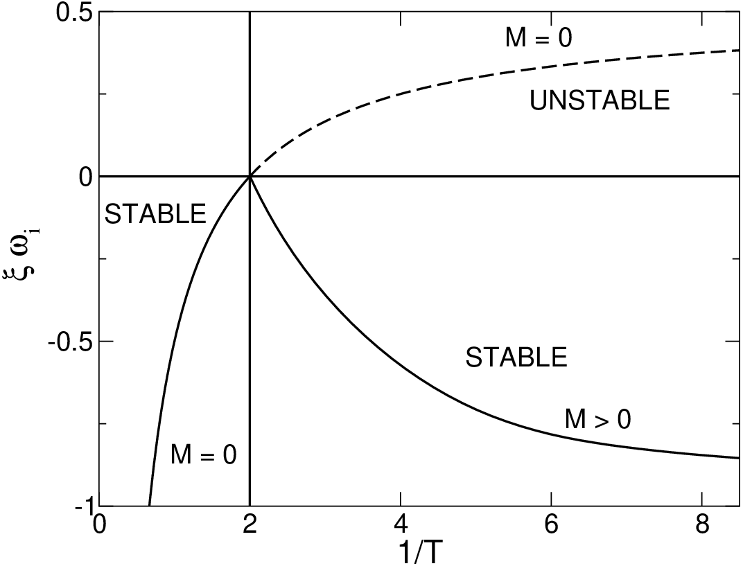
In conclusion, we find that dynamical and thermodynamical stability coincide. We note that the modes $n=\pm 1$ are associated with the magnetization (see Appendix A). Therefore, Eqs. (130) and (134) give the growth rate or the damping rate of the magnetization (see also Section 7). Starting from an unstable homogeneous distribution below the critical temperature ( $T<T_{c}$ ), there is first an exponential growth of the magnetization on a timescale $\sim\xi(T_{c}-T)^{-1}$ . Then, nonlinear terms come into play. Finally, the system relaxes towards a stable clustered state on a timescale $\sim(1/2)\xi(T_{c}-T)^{-1}$ . The fact that only the modes $n=\pm 1$ grow during the linear regime explains why we observe just one cluster in the numerical simulation of the mean field cosine Smoluchowski equation (see Figure 10 in Section 7). We also note that the relaxation is very slow close to the critical point. In fact, close to the critical point, the mean field approximation is not valid anymore due to the enhancement of fluctuations (see Section 10).

6 The linear response theory applied to the mean field Smoluchowski equation

In this section, we study the linear response of the BMF model to an external perturbation. Other applications of the linear response theory to systems with long-range interactions have been developed in Refs. [63, 64, 65].

6.1 The mean field Smoluchowski equation with an external potential

In the presence of an external potential $\Psi(\theta,t)$ , the mean field Smoluchowski equation becomes

\xi\frac{\partial\rho}{\partial t}=\frac{\partial}{\partial\theta}\left(T\frac{\partial\rho}{\partial\theta}+\rho\frac{\partial\Phi}{\partial\theta}+\rho\frac{\partial\Psi}{\partial\theta}\right),

(135)

with Eq. (12). We assume that the system has a homogeneous distribution $\rho=1/(2\pi)$ and we examine its response to a small external potential $\Psi(\theta,t)\ll 1$ . Since the perturbation is small, we can develop a linear response theory. The linearized Smoluchowski equation writes

\xi\frac{\partial\delta\rho}{\partial t}=\frac{\partial}{\partial\theta}\left(T\frac{\partial\delta\rho}{\partial\theta}+\rho\frac{\partial\delta\Phi}{\partial\theta}+\rho\frac{\partial\Psi}{\partial\theta}\right),

(136)

with Eq. (124). Since the external potential is introduced at $t=0$ (say), it is convenient to use Laplace transforms in time and Fourier transforms in space. The Fourier-Laplace transform of the perturbed density $\delta\rho(\theta,t)$ is defined by

\delta\tilde{\rho}_{n}(\omega)=\int_{0}^{2\pi}\frac{d\theta}{2\pi}\int_{0}^{+\infty}dt\,e^{-i(n\theta-\omega t)}\delta\rho(\theta,t).

(137)

This expression for the Laplace transform is valid for ${\rm Im}(\omega)$ sufficiently large. For the remaining part of the complex $\omega$ plane, it is defined by an analytic continuation. The inverse Fourier-Laplace transform is

\delta\rho(\theta,t)=\sum_{n}\int_{\cal C}\frac{d\omega}{2\pi}\,e^{i(n\theta-\omega t)}\delta\tilde{\rho}_{n}(\omega),

(138)

where the Laplace contour ${\cal C}$ in the complex $\omega$ plane must pass above all poles of the integrand. Similar definitions are introduced for the Fourier-Laplace transform of the perturbed potential.

Taking the Fourier-Laplace transform of Eqs. (124) and (136), and using Eq. (81), we obtain

\delta\tilde{\Phi}_{n}(\omega)=\frac{n^{2}\hat{u}_{n}}{i\xi\omega-n^{2}(T+\hat{u}_{n})}\tilde{\Psi}_{n}(\omega),

(139)

where we have assumed $\delta\Phi(\theta,t)=0$ at $t=0$ . The response function is defined by

\delta\tilde{\Phi}_{n}(\omega)=R_{n}(\omega)\tilde{\Psi}_{n}(\omega).

(140)

Therefore, we get

R_{n}(\omega)=\frac{n^{2}\hat{u}_{n}}{i\xi\omega-n^{2}(T+\hat{u}_{n})}.

(141)

The polarization function is defined by

\delta\tilde{\Phi}_{n}(\omega)=P_{n}(\omega)[\tilde{\Psi}_{n}(\omega)+\delta\tilde{\Phi}_{n}(\omega)],

(142)

yielding

P_{n}(\omega)=\frac{R_{n}(\omega)}{1+R_{n}(\omega)}=\frac{n^{2}\hat{u}_{n}}{i\xi\omega-Tn^{2}}.

(143)

Finally, the dielectric function is defined by

\epsilon_{n}(\omega)=1-P_{n}(\omega)=1-\frac{n^{2}\hat{u}_{n}}{i\xi\omega-Tn^{2}}.

(144)

We note the relations

R_{n}(\omega)=\frac{P_{n}(\omega)}{1-P_{n}(\omega)}=\frac{1-\epsilon_{n}(\omega)}{\epsilon_{n}(\omega)}.

(145)

The pure modes ( $\Psi=0$ ) correspond to $1/R_{n}(\omega)=\epsilon_{n}(\omega)=0$ . This returns the dispersion relation (126). The physical meaning of the response, polarization, and dielectric functions is further discussed in [5, 65].

6.2 The density response function

Another important quantity is the density response function defined by

\delta\tilde{\rho}_{n}(\omega)=\chi_{n}(\omega)\tilde{\Psi}_{n}(\omega).

(146)

According to Eqs. (81) and (140) it is related to the response function by $R_{n}(\omega)=2\pi\hat{u}_{n}\chi_{n}(\omega)$ . From Eq. (141) we get

\chi_{n}(\omega)=\frac{1}{2\pi}\frac{n^{2}}{i\xi\omega-n^{2}(T+\hat{u}_{n})}.

(147)

The previous relation gives the dynamical density response function. We now consider the static case. We start from the mean field Boltzmann distribution (62), introduce an external field, and consider the weak field limit. The static response function is defined by

\delta\tilde{\rho}_{n}=\chi_{n}\tilde{\Psi}_{n}.

(148)

Since the Boltzmann distribution is the steady state of the mean field Smoluchowski equation, the previous study remains valid provided that we set $\omega=0$ . Therefore $\chi_{n}=\chi_{n}(0)$ yielding

\chi_{n}=-\frac{1}{2\pi}\frac{1}{T+\hat{u}_{n}}.

(149)

Similar results hold for $R_{n}$ , $P_{n}$ , and $\epsilon_{n}$ . These results can also be obtained as in Appendix C.

6.3 The magnetization

We assume that the external potential is of the form

\Psi(\theta,t)=-h(t)\cos\theta,

(150)

where $h$ may be interpreted as a magnetic field acting in the $x$ -direction (see Section 4.6). Its Fourier-Laplace transform is

\tilde{\Psi}_{n}(\omega)=-\frac{1}{2}\tilde{h}(\omega)(\delta_{n,1}+\delta_{n,-1}).

(151)

On the other hand, from Eq. (13), the fluctuations of the potential can be expressed in terms of the fluctuations of the magnetization as

\delta\Phi(\theta,t)=-M_{x}(t)\cos\theta-M_{y}(t)\sin\theta.

(152)

Taking the Fourier-Laplace transform of this equation, we obtain

	$\displaystyle\delta\tilde{\Phi}_{n}(\omega)=-\frac{1}{2}(\tilde{M}_{x}+i\tilde{M}_{y})(\omega)\delta_{n,-1}$
	$\displaystyle-\frac{1}{2}(\tilde{M}_{x}-i\tilde{M}_{y})(\omega)\delta_{n,1}.$		(153)

From Eqs. (139) and (151), we see that $\delta\tilde{\Phi}_{1}(\omega)=\delta\tilde{\Phi}_{-1}(\omega)$ . According to Eq. (153), this implies that $\tilde{M}_{y}(\omega)=0$ . Therefore, Eq. (153) reduces to

\delta\tilde{\Phi}_{n}(\omega)=-\frac{1}{2}\tilde{M}_{x}(\omega)(\delta_{n,1}+\delta_{n,-1}).

(154)

We can rewrite Eq. (140) as

\tilde{M}_{x}(\omega)=R(\omega)\tilde{h}(\omega),

(155)

with

R(\omega)=-\frac{T_{c}}{i\xi\omega-(T-T_{c})}.

(156)

We also have

\tilde{M}_{x}(\omega)=P(\omega)[\tilde{h}(\omega)+\tilde{M}_{x}(\omega)],

(157)

with

P(\omega)=\frac{R(\omega)}{1+R(\omega)}=-\frac{T_{c}}{i\xi\omega-T}.

(158)

The dielectric function is

\epsilon(\omega)=1-P(\omega)=1+\frac{T_{c}}{i\xi\omega-T}.

(159)

We note the relations

R(\omega)=\frac{P(\omega)}{1-P(\omega)}=\frac{1-\epsilon(\omega)}{\epsilon(\omega)}.

(160)

6.4 The response to a pulse

We consider the response of the system to a magnetic “pulse” localized at $t=0$ . It can be represented by the Dirac distribution

h(t)=\delta(t).

(161)

The Laplace transform of the magnetic field is

\tilde{h}(\omega)=1.

(162)

According to Eq. (155), the perturbation caused by a pulse is equal to the response function

\tilde{M}_{x}(\omega)=R(\omega).

(163)

Taking the inverse Laplace transform of Eq. (156), we obtain

{M}_{x}(t)=R(t)=-\int_{\cal C}\frac{d\omega}{2\pi}e^{-i\omega t}\frac{T_{c}}{i\xi\omega-(T-T_{c})}.

(164)

The integral can be easily calculated with the residue theorem leading to

{M}_{x}(t)=R(t)=\frac{T_{c}}{\xi}e^{-(T-T_{c})t/\xi}.

(165)

The polarization function can be calculated similarly yielding

P(t)=\frac{T_{c}}{\xi}e^{-Tt/\xi}.

(166)

In the stable case $T>T_{c}$ , the perturbation $M_{x}(t)$ is damped exponentially rapidly (it tends to $0$ for $t\rightarrow+\infty$ ) and in the unstable case $T<T_{c}$ , the perturbation grows exponentially rapidly. This is of course consistent with the results of Section 5. The linear response theory is another manner to study the dynamical stability of a system.

6.5 The response to a step function

We consider the response of the system to a constant magnetic field that is “switched on” suddenly at $t=0$ . It can be represented by a step function

h(t)=H(t)h,

(167)

where $H(t)=0$ for $t<0$ and $H(t)=1$ for $t>0$ (Heaviside function). The Laplace transform of the magnetic field is

\tilde{h}(\omega)=\frac{i}{\omega}h.

(168)

According to Eq. (155), the perturbation caused by a step function is

\tilde{M}_{x}(\omega)=R(\omega)\frac{i}{\omega}h.

(169)

Taking the inverse Laplace transform of this equation and using Eq. (156), we obtain

{M}_{x}(t)=-h\int_{\cal C}\frac{d\omega}{2\pi}e^{-i\omega t}\frac{T_{c}}{i\xi\omega-(T-T_{c})}\frac{i}{\omega}.

(170)

The integral can be easily calculated with the residue theorem leading to

{M}_{x}(t)=\frac{T_{c}}{T-T_{c}}\left[1-e^{-(T-T_{c})t/\xi}\right]h.

(171)

In the stable case $T>T_{c}$ , the perturbation $M_{x}(t)$ tends to the asymptotic value

({M}_{x})_{\infty}=\frac{T_{c}}{T-T_{c}}h,

(172)

which corresponds to the equilibrium magnetization of the BMF model under a weak magnetic field (see Section 4.6). It arises here as the pole of the integral (170) at $\omega=0$ . We note that the magnetic susceptibility is

\chi_{M}=R=-\pi\chi=\frac{T_{c}}{T-T_{c}}.

(173)

In the unstable case $T<T_{c}$ , the perturbation grows exponentially rapidly. Of course, the linear response theory ceases to be valid when the perturbation has grown significatively, so the expressions (165) and (171) are only valid for sufficiently “short” times in the unstable case.

6.6 The evolution of the magnetization in the presence of a magnetic field

The previous results may be obtained in a more synthetic manner as follows. If we decompose the density perturbation $\delta\rho(\theta,t)$ in Fourier modes according to Eq. (269) and substitute this decomposition in the linearized Smoluchowski equation (136), we obtain the modal equations

\displaystyle\xi\frac{d\delta\hat{\rho}_{n}}{dt}+n^{2}(T+\hat{u}_{n})\delta\hat{\rho}_{n}=-n^{2}\rho\hat{\Psi}_{n}(t).

(174)

The different modes evolve as

\displaystyle\delta\hat{\rho}_{n}(t)=-\frac{n^{2}\rho}{\xi}\int_{0}^{t}\hat{\Psi}_{n}(s)e^{-\frac{n^{2}}{\xi}(T+\hat{u}_{n})(t-s)}\,ds,

(175)

where we have assumed that $\delta\hat{\rho}_{n}(0)=0$ . When the external potential is a step function $\hat{\Psi}_{n}(t)=H(t)\hat{\Psi}_{n}$ , we get

\displaystyle\delta\hat{\rho}_{n}(t)=-\frac{\rho\hat{\Psi}_{n}}{T+\hat{u}_{n}}\left[1-e^{-n^{2}(T+\hat{u}_{n})t/\xi}\right],

(176)

which tends to

\displaystyle\delta\hat{\rho}_{n}^{\infty}=-\frac{\rho\hat{\Psi}_{n}}{T+\hat{u}_{n}},

(177)

for $t\rightarrow+\infty$ (for the stable modes). We recover the expression (149) of the static density response function. These relations generalize the preceding results.

In the case of the cosine potential (2), and for an external potential of the form (150), the modal equations become

\displaystyle\xi\frac{d\delta\hat{\rho}_{n}}{dt}+Tn^{2}\delta\hat{\rho}_{n}=0,\qquad(n\neq\pm 1)

(178)

\displaystyle\xi\frac{d\delta\hat{\rho}_{\pm 1}}{dt}+(T-T_{c})\delta\hat{\rho}_{\pm 1}=\frac{1}{4\pi}h(t).

(179)

We see that the modes $n\neq\pm 1$ are damped exponentially rapidly as $e^{-Tn^{2}t/\xi}$ . Only the modes $n=\pm 1$ have a non trivial evolution. Recalling that the modes $\delta\hat{\rho}_{\pm 1}$ are related to the magnetization (see Appendix A), we can rewrite Eq. (179) in the form

\displaystyle\xi\frac{d{\bf M}}{dt}+(T-T_{c}){\bf M}=T_{c}{\bf h},

(180)

where ${\bf M}=M_{x}+iM_{y}$ and ${\bf h}=h$ . From this equation, we can establish the results of Eqs. (165), (171), and (172).

7 The evolution of the mean magnetization in the inhomogeneous phase

In the previous sections, we have considered the linear dynamical stability of a steady state of the mean field cosine Smoluchowski equation, and the linear response of the system to a weak external potential. We now turn to the nonlinear evolution of the mean field cosine Smoluchowski equation. This equation exhibits an interesting process of self-organization. Indeed, for $T<T_{c}$ , the spatially homogeneous phase is unstable and the system evolves towards an equilibrium state with a spatially inhomogeneous distribution (clustered phase). This process of self-organization is illustrated on Figure 10 for $T=1/4$ . In this section, we analytically study the evolution of the magnetization close to the critical point.

7.1 The modal decomposition of the mean field cosine Smoluchowski equation

In the mean field approximation, the evolution of the density profile $\rho(\theta,t)$ is given by the cosine Smoluchowski equation (39). Decomposing the density profile in Fourier modes according to Eq. (269), and using the identities of Appendix A, we obtain a hierarchy of coupled ordinary differential equations

\displaystyle\xi\frac{d\hat{\rho}_{n}}{dt}+Tn^{2}\hat{\rho}_{n}=-2\pi n\sum_{m}m\hat{\rho}_{m}\hat{u}_{m}\hat{\rho}_{n-m}.

(181)

For the cosine potential, using Eq. (82), the hierarchy of equations (181) takes the form

\displaystyle\xi\frac{d\hat{\rho}_{n}}{dt}+Tn^{2}\hat{\rho}_{n}=\pi n(\hat{\rho}_{1}\hat{\rho}_{n-1}-\hat{\rho}_{-1}\hat{\rho}_{n+1}).

(182)

The modes $\hat{\rho}_{\pm 1}$ are directly related to the components of the magnetization ${\bf M}$ (see Appendix A). This infinite hierarchy of equations is equivalent to the mean field cosine Smoluchowski equation (39). A good approximation of the solution can be obtained by taking a sufficient number of modes ${\cal N}\gg 1$ and closing the hierarchy by imposing the condition $\hat{\rho}_{\pm{\cal N}}=0$ . The density profile can then be reconstructed from Eq. (269). This is the numerical procedure used in [17] to obtain the result of Figure 10.

At equilibrium, the hierarchy of equations (182) reduces to

\displaystyle Tn^{2}\hat{\rho}_{n}=\pi n(\hat{\rho}_{1}\hat{\rho}_{n-1}-\hat{\rho}_{-1}\hat{\rho}_{n+1}).

(183)

Using $\hat{\rho}_{n}=I_{n}(\beta M)/[2\pi I_{0}(\beta M)]$ according to Eqs. (67) and (270), we find that Eq. (183) is equivalent to the recursive relation $2nI_{n}(x)/x=I_{n-1}(x)-I_{n+1}(x)$ satisfied by the Bessel functions. On the other hand, considering a small perturbation $\delta\hat{\rho}_{n}\propto e^{\omega_{i}t}$ around the equilibrium state (assumed to be symmetric with respect to the $x$ -axis), linearizing Eq. (182), and using the identities of Appendix A, we obtain the eigenvalue equations

	$\displaystyle\xi\omega_{i}\delta M_{x}^{(n)}$	$\displaystyle=$	$\displaystyle-Tn^{2}\delta M_{x}^{(n)}+\frac{1}{2}nM_{x}[\delta M_{x}^{(n-1)}-\delta M_{x}^{(n+1)}]$		(184)
		$\displaystyle+$	$\displaystyle\frac{1}{2}n\delta M_{x}[M_{x}^{(n-1)}-M_{x}^{(n+1)}],$		(184)

	$\displaystyle\xi\omega_{i}\delta M_{y}^{(n)}$	$\displaystyle=$	$\displaystyle-Tn^{2}\delta M_{y}^{(n)}+\frac{1}{2}nM_{x}[\delta M_{y}^{(n-1)}-\delta M_{y}^{(n+1)}]$		(185)
		$\displaystyle+$	$\displaystyle\frac{1}{2}n\delta M_{y}[M_{x}^{(n-1)}+M_{x}^{(n+1)}].$		(185)

These equations are equivalent to the eigenvalue problem written in the form of a differential equation in Section 5.2.

7.2 The closure of the hierarchy close to the critical point

When $T<T_{c}$ , the equilibrium distribution is spatially inhomogeneous ( $M\neq 0$ ) but close to the critical point $T\rightarrow T_{c}^{+}$ the magnetization $M\rightarrow 0$ . We assume that the initial magnetization is small so that $M(t)$ remains small during all the evolution. In that case, analytical results can be obtained. Indeed, according to Eq. (182), the density modes scale as $\hat{\rho}_{n}\sim M^{n}$ . Therefore, when $M\ll 1$ , the modes of higher and higher order become less and less important. After a transient regime of duration $2\xi/n^{2}$ , the modes $n>0$ are given by

\displaystyle\hat{\rho}_{n}\sim\frac{2\pi}{n}\hat{\rho}_{1}\hat{\rho}_{n-1}\sim{(2\pi)^{n-1}}\frac{1}{n!}\hat{\rho}_{1}^{n},

(186)

and the modes $n<0$ by

\displaystyle\hat{\rho}_{n}\sim-\frac{2\pi}{n}\hat{\rho}_{-1}\hat{\rho}_{n+1}\sim{(2\pi)^{|n|-1}}\frac{1}{|n|!}\hat{\rho}_{-1}^{|n|}.

(187)

In particular, for $n=2$ , we get

\displaystyle\hat{\rho}_{\pm 2}\sim{\pi}\hat{\rho}_{\pm 1}^{2}.

(188)

This shows that the second mode is slaved to the first (this corresponds to an adiabatic approximation). In that case, we obtain the closed equations

\displaystyle\xi\frac{d\hat{\rho}_{\pm 1}}{dt}+(T-T_{c})\hat{\rho}_{\pm 1}=-{\pi^{2}}\hat{\rho}_{\mp 1}\hat{\rho}_{\pm 1}^{2},

(189)

Using the results of Appendix A, they can be rewritten in terms of the components $M_{x}$ and $M_{y}$ of the magnetization as

\displaystyle\xi\frac{dM_{x}}{dt}+(T-T_{c})M_{x}=-\frac{M^{2}}{4}M_{x},

(190)

\displaystyle\xi\frac{dM_{y}}{dt}+(T-T_{c})M_{y}=-\frac{M^{2}}{4}M_{y},

(191)

where $M=(M_{x}^{2}+M_{y}^{2})^{1/2}$ . Introducing the complex magnetization ${\bf M}=M_{x}+iM_{y}$ , Eqs. (190) and (191) may be combined into a single equation

\displaystyle\xi\frac{d{\bf M}}{dt}=-(T-T_{c}){\bf M}-\frac{M^{2}}{4}{\bf M}.

(192)

We note that

\displaystyle\xi\frac{d{\bf M}}{dt}=-\frac{1}{2}\frac{\partial F}{\partial{\bf M}},

(193)

where $F(M)$ is the approximate expression (101) of the free energy close to equilibrium for $T\rightarrow T_{c}^{-}$ . For $T>T_{c}$ , the evolution of the magnetization close to equilibrium is given by Eq. (192) without the cubic term. In that case, the free energy is given by Eq. (100).

The steady states of Eq. (193) correspond to extrema of free energy ( $F^{\prime}(M)=0$ ). Since

\displaystyle\dot{F}=-\frac{1}{2\xi}\left(\frac{\partial F}{\partial{\bf M}}\right)^{2}\leq 0,

(194)

the magnetization ${\bf M}(t)$ relaxes towards a minimum of free energy (maxima of free energy are unstable). Considering a small perturbation about a steady state of Eq. (193), we find that the perturbation evolves as $\delta M\propto e^{\omega_{i}t}$ with $\omega_{i}=-\frac{1}{2\xi}F^{\prime\prime}(M)$ .

7.3 The evolution of the mean magnetization close to the critical point

For sufficiently short times, and for sufficiently small initial magnetization, we can neglect the cubic term in Eq. (192). This corresponds to the linear regime. The resulting equation

\displaystyle\xi\frac{d{\bf M}}{dt}=-(T-T_{c}){\bf M},

(195)

can be integrated into

\displaystyle M(t)\simeq M_{0}e^{(T_{c}-T)t/\xi},

(196)

returning the exponential rate (130). For $T>T_{c}$ , the perturbation is damped at a rate $\omega_{i}=(T_{c}-T)/\xi<0$ and the magnetization tends to zero (homogeneous phase). In that case, the solution (196) is valid for all times. For $T<T_{c}$ , the perturbation grows at a rate $\omega_{i}=(T_{c}-T)/\xi>0$ . This growth is limited by nonlinear effects represented by the cubic term in Eq. (192) so that a magnetized state is finally reached (inhomogeneous phase). A simple analytical solution describing this saturation may be obtained [17]. From Eq. (192), we find that the evolution of the modulus of the magnetization is governed by the equation

\displaystyle\xi\frac{dM}{dt}+(T-T_{c})M=-\frac{M^{3}}{4}.

(197)

This equation is readily solved (it may be convenient to use $M^{2}$ as a variable) with the initial condition $M(0)=M_{0}$ . We obtain

\displaystyle M(t)=\frac{M}{\sqrt{1+\left(\frac{M^{2}}{M_{0}^{2}}-1\right)e^{-2(T_{c}-T)t/\xi}}},

(198)

where

\displaystyle M=2\sqrt{T_{c}-T},

(199)

is the asymptotic value of the magnetization reached for $t\rightarrow+\infty$ . This returns the equilibrium value of the magnetization (76) close to the critical point. The magnetization relaxes towards its equilibrium value as

\displaystyle M(t)\simeq M\left[1-\frac{1}{2}\left(\frac{M^{2}}{M_{0}^{2}}-1\right)e^{-2(T_{c}-T)t/\xi}\right],

(200)

returning the damping rate (134). On the other hand, for $t\rightarrow 0$ , one has

\displaystyle M(t)\simeq M_{0}\left[1+\frac{1}{4\xi}(M^{2}-M_{0}^{2}){t}\right].

(201)

The magnetization increases if $M_{0}<M$ and decreases if $M_{0}>M$ . When $M_{0}\ll M$ , we recover the result of Eq. (196). The analytical solution (198) describes the complete evolution of the magnetization close to the critical point $T_{c}$ , from its initial growth to its convergence towards its equilibrium value (see Figure 11).

Solving Eqs. (190) and (191) with Eq. (198), we get

\displaystyle M_{x}(t)=\frac{\frac{M_{x}(0)}{M_{0}}M}{\sqrt{1+\left(\frac{M^{2}}{M_{0}^{2}}-1\right)e^{-2(T_{c}-T)t/\xi}}},

(202)

\displaystyle M_{y}(t)=\frac{\frac{M_{y}(0)}{M_{0}}M}{\sqrt{1+\left(\frac{M^{2}}{M_{0}^{2}}-1\right)e^{-2(T_{c}-T)t/\xi}}}.

(203)

We see that if $M_{x}(0)=M_{y}(0)$ initially, then $M_{x}(t)=M_{y}(t)$ for all times. Similarly, if $M_{y}(0)=0$ initially then $M_{y}(t)=0$ for all times. More generally, writing $M_{x}(t)=M(t)\cos\phi(t)$ and $M_{y}(t)=M(t)\sin\phi(t)$ , we see that $\tan\phi(t)=M_{y}(0)/M_{x}(0)$ so that the phase is conserved. As a result, we can take $\phi=0$ without loss of generality. In that case, $M_{y}(t)=0$ and $M_{x}(t)=M(t)$ . The density profile close to the critical point can be written as

\displaystyle\rho(\theta,t)=\frac{1}{2\pi}+\frac{1}{\pi}M(t)\cos\theta,

(204)

where $M(t)$ is given by Eq. (198).

At $T=T_{c}$ , the solution of Eq. (192) is

\displaystyle M(t)={M_{0}\over\sqrt{1+{M_{0}^{2}t\over 2\xi}}}.

(205)

The magnetization tends to zero algebraically as $t^{-1/2}$ for $t\rightarrow+\infty$ (assuming that the mean field approximation is correct which is not the case close to $T_{c}$ as we shall see shortly). Solving Eqs. (190) and (191) with Eq. (205), we get

\displaystyle M_{x}(t)={M_{x}(0)\over\sqrt{1+{M_{0}^{2}t\over 2\xi}}},\qquad M_{y}(t)={M_{y}(0)\over\sqrt{1+{M_{0}^{2}t\over 2\xi}}}.

(206)

Remark: We have truncated the hierarchy of equations (182) by using the approximation (188). This is valid close to the critical point $T_{c}$ . Another approach would be to truncate the hierarchy of equations at the level of $\hat{\rho}_{\pm 2}$ by taking $\hat{\rho}_{\pm 3}=0$ . In that case, we get the coupled equations

\displaystyle\xi\frac{d\hat{\rho}_{\pm 1}}{dt}+(T-T_{c})\hat{\rho}_{\pm 1}=-\pi\hat{\rho}_{\mp 1}\hat{\rho}_{\pm 2},

(207)

\displaystyle\xi\frac{d\hat{\rho}_{\pm 2}}{dt}+4T\hat{\rho}_{\pm 2}=2\pi\hat{\rho}_{\pm 1}^{2}.

(208)

This system of equations is closed but it does not seem to admit a simple analytical solution. If we replace Eq. (208) by its asymptotic expression $\hat{\rho}_{\pm 2}=\pi\hat{\rho}_{\pm 1}^{2}$ and substitute this relation in Eq. (207), we recover Eq. (189). However, Eqs. (207)-(208) are more general that Eq. (189) because they do not rely on an adiabatic assumption.

8 The temporal correlations of the magnetization in the homogeneous phase

8.1 The density fluctuation spectrum and the structure factor

In the previous sections, we have used a mean field approximation which amounts to neglecting fluctuations. For large values of $N$ , this is a good approximation for systems with long-range interactions, except close to a critical point. In this section, we study the correlations of the magnetization in the homogeneous phase and show that they diverge as $T\rightarrow T_{c}^{+}$ . To that purpose, we return to the stochastic Smoluchowski equation (51). Since the noise is weak when $N\gg 1$ , we can consider small fluctuations $\delta\rho(\theta,t)$ and $\delta\Phi(\theta,t)$ about the homogeneous steady state $\rho=1/(2\pi)$ and $\Phi=1$ . The linearized equation for the fluctuations is

\displaystyle\xi\frac{\partial\delta\rho}{\partial t}=T\frac{\partial^{2}\delta\rho}{\partial\theta^{2}}+\rho\frac{\partial^{2}\delta\Phi}{\partial\theta^{2}}+\sqrt{\frac{2\xi T\rho}{N}}\frac{\partial R}{\partial\theta}(\theta,t),

(209)

with Eq. (124). We introduce the Fourier transform of the density fluctuations in space and time

\delta\hat{\rho}_{n}(\omega)=\int_{0}^{2\pi}\frac{d\theta}{2\pi}\int_{-\infty}^{+\infty}\frac{dt}{2\pi}\,e^{-i(n\theta-\omega t)}\delta\rho(\theta,t).

(210)

The inverse Fourier transform is

\delta\rho(\theta,t)=\sum_{n=-\infty}^{+\infty}\int_{-\infty}^{+\infty}{d\omega}\,e^{i(n\theta-\omega t)}\delta\hat{\rho}_{n}(\omega).

(211)

We use similar notations for the fluctuations of the potential $\delta\Phi(\theta,t)$ and for the noise $R(\theta,t)$ .

Taking the Fourier transform of Eqs. (124) and (209), and using Eq. (81), we find that the fluctuations of the density induced by the noise are given by

\displaystyle\delta\hat{\rho}_{n}(\omega)=in\sqrt{\frac{2\xi T\rho}{N}}\frac{1}{Z_{n}(\omega)}\hat{R}_{n}(\omega),

(212)

where

\displaystyle Z_{n}(\omega)=Tn^{2}+\hat{u}_{n}n^{2}-i\xi\omega.

(213)

Without noise ( ${R}={0}$ ), we must have $Z_{n}(\omega)=0$ and we recover the dispersion relation (126) corresponding to a pure mode.

For a Gaussian white noise, $\langle\hat{R}_{n}(\omega)\rangle=0$ and

\displaystyle\langle\hat{R}_{n}(\omega)\hat{R}_{n^{\prime}}(\omega^{\prime})\rangle=\frac{1}{(2\pi)^{2}}\delta_{n,-n^{\prime}}\delta(\omega+\omega^{\prime}).

(214)

Therefore, the correlations of the fluctuations are

\displaystyle\langle\delta\hat{\rho}_{n}(\omega)\delta\hat{\rho}_{n^{\prime}}(\omega^{\prime})\rangle=\frac{1}{(2\pi)^{2}}\frac{2\xi T\rho}{N}\frac{n^{2}}{|Z_{n}(\omega)|^{2}}\delta_{n,-n^{\prime}}\delta(\omega+\omega^{\prime}).

The density fluctuation spectrum is defined by

\displaystyle\langle\delta\hat{\rho}_{n}(\omega)\delta\hat{\rho}_{n^{\prime}}(\omega^{\prime})\rangle=\frac{1}{2\pi}S_{n}(\omega)\delta_{n,-n^{\prime}}\delta(\omega+\omega^{\prime}).

(216)

According to Eqs. (213) and (8.1), we find that the density fluctuation spectrum is the Lorenzian

\displaystyle S_{n}(\omega)=\frac{1}{2\pi^{2}}\frac{\xi Tn^{2}}{\xi^{2}\omega^{2}+n^{4}(T+\hat{u}_{n})^{2}}.

(217)

We note that it becomes more and more narrow as we approach the neutral mode defined by Eq. (128). The temporal correlation function of the Fourier components of the density fluctuations is given by

\displaystyle\langle\delta\hat{\rho}_{n}(t)\delta\hat{\rho}_{n^{\prime}}(t^{\prime})\rangle=\frac{n^{2}}{(2\pi)^{2}}\frac{2\xi T\rho}{N}\delta_{n,-n^{\prime}}\int_{-\infty}^{+\infty}d\omega\,\frac{e^{-i\omega(t-t^{\prime})}}{|Z_{n}(\omega)|^{2}}.

The integral over $\omega$ can be easily performed by using the Cauchy residue theorem yielding

\displaystyle\langle\delta\hat{\rho}_{n}(t)\delta\hat{\rho}_{n^{\prime}}(t^{\prime})\rangle=\frac{1}{N}\frac{T\rho^{2}}{T+\hat{u}_{n}}\delta_{n,-n^{\prime}}e^{-n^{2}(T+\hat{u}_{n})|t-t^{\prime}|/\xi}.

The equal time correlation function is

\displaystyle\langle\delta\hat{\rho}_{n}\delta\hat{\rho}_{n^{\prime}}\rangle=\frac{1}{N}\frac{T\rho^{2}}{T+\hat{u}_{n}}\delta_{n,-n^{\prime}}.

(220)

The structure factor is defined by

\displaystyle\langle\delta\hat{\rho}_{n}\delta\hat{\rho}_{n^{\prime}}\rangle=\frac{1}{2\pi}S_{n}\delta_{n,-n^{\prime}}.

(221)

According to Eq. (220), it is given by

\displaystyle S_{n}=\frac{1}{2\pi}\frac{T}{T+\hat{u}_{n}}.

(222)

We note that the structure factor diverges at the neutral mode defined by Eq. (128). This is manifested by a peak in the spectrum.

The results of this section can be obtained in different manners as shown in Appendices C and D.

8.2 Application to the cosine potential

The foregoing expressions can be simplified for the cosine potential (2) using Eq. (82). The density fluctuation spectrum (217) can be written as

\displaystyle S_{n}(\omega)=\frac{1}{2\pi^{2}}\frac{\xi Tn^{2}}{\xi^{2}\omega^{2}+n^{4}T^{2}}\qquad(n\neq\pm 1),

(223)

\displaystyle S_{\pm 1}(\omega)=\frac{1}{2\pi^{2}}\frac{\xi T}{\xi^{2}\omega^{2}+(T-T_{c})^{2}}.

(224)

The Lorenzian $S_{\pm 1}(\omega)$ becomes more and more narrow as we approach the critical temperature $T\rightarrow T_{c}$ . The temporal correlation function of the density fluctuations for the stable modes $n\neq\pm 1$ is

\displaystyle\langle\delta\hat{\rho}_{n}(t)\delta\hat{\rho}_{n^{\prime}}(t^{\prime})\rangle=\frac{1}{N}\rho^{2}e^{-Tn^{2}|t-t^{\prime}|/\xi}\delta_{n,-n^{\prime}}.

(225)

For the unstable modes $n=\pm 1$ , we get

\displaystyle\langle\delta\hat{\rho}_{\pm 1}(t)\delta\hat{\rho}_{n^{\prime}}(t^{\prime})\rangle=\frac{1}{N}\frac{T\rho^{2}}{T-T_{c}}e^{-(T-T_{c})|t-t^{\prime}|/\xi}\delta_{n^{\prime},\mp 1}.

The equal time correlation function is

\displaystyle\langle\delta\hat{\rho}_{n}\delta\hat{\rho}_{n^{\prime}}\rangle=\frac{1}{N}\rho^{2}\delta_{n,-n^{\prime}}

(227)

for the stable modes $n\neq\pm 1$ and

\displaystyle\langle\delta\hat{\rho}_{\pm 1}\delta\hat{\rho}_{n^{\prime}}\rangle=\frac{1}{N}\frac{T\rho^{2}}{T-T_{c}}\delta_{n^{\prime},\mp 1}

(228)

for the unstable modes $n=\pm 1$ . The structure factor is

\displaystyle S_{n\neq\pm 1}=\frac{1}{2\pi},\qquad S_{\pm 1}=\frac{1}{2\pi}\frac{T}{T-T_{c}}.

(229)

It diverges at the critical point $T_{c}$ . Using the relations of Appendix A, we can express these results in terms of the magnetization. We obtain $\langle M_{x}(t)M_{y}(t^{\prime})\rangle=0$ and $\langle M_{x}(t)M_{x}(t^{\prime})\rangle=\langle M_{y}(t)M_{y}(t^{\prime})\rangle$ with

\displaystyle\langle M_{x}(t)M_{x}(t^{\prime})\rangle=\frac{T}{2N(T-T_{c})}e^{-(T-T_{c})|t-t^{\prime}|/\xi}.

(230)

Taking $t^{\prime}=t$ , we find that the equal time correlation function of the magnetization is given by Eq. (105).

The physical content of Eq. (230) is very instructive. Considering the temporal factor in Eq. (230), we see that the correlations decay for $T>T_{c}$ with the rate (130) given by the mean field theory, i.e. by the deterministic mean field Smoluchowski equation (39) without noise. However, as we approach the critical temperature $T_{c}$ , the amplitude of the fluctuations diverges like $(T-T_{c})^{-1}$ so that the phase transition should occur for $T$ strictly above $T_{c}$ . Indeed, the fluctuations become large before ordinary stability theory predicts growth. We had previously reached this conclusion from the YBG hierarchy [17, 56]. These results imply that the mean field approximation breaks down close to the critical point⁵⁵ 5 Indeed, the limits $N\rightarrow+\infty$ (mean field) and $T\rightarrow T_{c}$ do not commute (see Appendix D). and that the instability triggering the phase transition occurs sooner than what is predicted by the mean field theory (i.e. by the stability analysis of the mean field Smoluchowski equation). Similar results have been reported for self-gravitating systems [52, 66, 67].

8.3 The fluctuation-dissipation theorem

There exist an important relation between the correlation function and the response of the system to an external perturbation. This is the so-called fluctuation-dissipation theorem [68]. It can be derived at a very general level but it is interesting to obtain it explicitly in the present model.

Comparing Eqs. (147) and (217), we find that the density fluctuation spectrum is related to the density response function by the relation

\displaystyle S_{n}(\omega)=-\frac{T}{\pi\omega}{\rm Im}\chi_{n}(\omega).

(231)

Similarly, comparing Eqs. (149) and (222), we find that the structure factor is related to the susceptibility by

\displaystyle S_{n}=-T\chi_{n}.

(232)

This identity can also be derived from Eq. (231) by using $S_{n}=\int S_{n}(\omega)\,d\omega$ .

For the cosine potential, we can obtain the relation (231) with $n=\pm 1$ by comparing Eqs. (156) and (224) and recalling that $R(\omega)=-\pi\chi(\omega)$ . Similarly, we can obtain the relation (232) with $n=\pm 1$ by comparing Eq. (173) and (229-b). Finally, using $N\langle M^{2}\rangle=2\pi S_{\pm 1}$ and $\chi_{M}=R_{\pm 1}=-\pi\chi_{\pm 1}$ , we check the equivalence between Eqs. (122) and (232).

9 The fluctuations of the magnetization in the homogeneous phase

9.1 The modal decomposition of the linearized stochastic cosine Smoluchowski equation

When $T>T_{c}$ (homogeneous phase) and $N\gg 1$ , the fluctuations of the density $\delta\rho(\theta,t)$ about the equilibrium distribution $\rho=1/(2\pi)$ are small. Their evolution is described by the linearized stochastic cosine Smoluchowski equation (209) with Eq. (124). Decomposing the density fluctuations $\delta\rho(\theta,t)$ in Fourier modes according to Eq. (269), and using Eq. (81), we find that the evolution of the different modes is given by

\displaystyle\xi\frac{d\delta\hat{\rho}_{n}}{dt}+n^{2}(T+\hat{u}_{n})\delta\hat{\rho}_{n}=in\sqrt{\frac{\xi T}{\pi N}}\,\hat{R}_{n}(t),

(233)

where $\hat{R}_{n}(t)$ is the Fourier transform of $R(\theta,t)$ . This is a Gaussian white noise with zero mean $\langle\hat{R}_{n}(t)\rangle=0$ and correlator

\displaystyle\langle\hat{R}_{n}(t)\hat{R}_{n^{\prime}}(t^{\prime})\rangle=\frac{1}{2\pi}\delta_{n,-n^{\prime}}\delta(t-t^{\prime}).

(234)

For the cosine potential (2), using Eq. (82), we get

\displaystyle\xi\frac{d\delta\hat{\rho}_{n}}{dt}+n^{2}T\delta\hat{\rho}_{n}=in\sqrt{\frac{\xi T}{\pi N}}\,\hat{R}_{n}(t),\quad(n\neq\pm 1)

(235)

\displaystyle\xi\frac{d\delta\hat{\rho}_{\pm 1}}{dt}+(T-T_{c})\delta\hat{\rho}_{\pm 1}=\pm i\sqrt{\frac{\xi T}{\pi N}}\,\hat{R}_{\pm 1}(t).

(236)

9.2 The Langevin equation for the fluctuations of the magnetization

From Eq. (236), using the relations of Appendix A, we find that the evolution of the fluctuations of the magnetization is given by

\displaystyle\xi\frac{dM_{x}}{dt}+(T-T_{c})M_{x}=\sqrt{\frac{\xi T}{N}}R_{x}(t),

(237)

\displaystyle\xi\frac{dM_{y}}{dt}+(T-T_{c})M_{y}=\sqrt{\frac{\xi T}{N}}R_{y}(t),

(238)

where $R_{x}(t)=i\sqrt{\pi}(\hat{R}_{1}-\hat{R}_{-1})$ and $R_{y}(t)=-\sqrt{\pi}(\hat{R}_{1}+\hat{R}_{-1})$ are Gaussian white noises with $\langle{R}_{i}(t)\rangle={0}$ and $\langle R_{i}(t)R_{j}(t^{\prime})\rangle=\delta_{ij}\delta(t-t^{\prime})$ . The magnetization vector ${\bf M}=M_{x}+iM_{y}$ satisfies a Langevin equation of the form

\displaystyle\xi\frac{d{\bf M}}{dt}+(T-T_{c}){\bf M}=\sqrt{\frac{\xi T}{N}}{\bf R}(t),

(239)

where ${\bf R}=R_{x}+iR_{y}$ . Equation (239) can be rewritten as

\displaystyle\xi\frac{d{\bf M}}{dt}=-\frac{1}{2}\frac{\partial F}{\partial{\bf M}}+\sqrt{\frac{\xi T}{N}}{\bf R}(t),

(240)

where $F({\bf M})$ is the approximate expression (100) of the free energy in the homogeneous phase when $M\ll 1$ .

9.3 The Fokker-Planck equation for the fluctuations of the magnetization

The Langevin equation (239) for the fluctuations of the magnetization defines an Ornstein-Uhlenbeck process. The Fokker-Planck equation governing the evolution of the distribution $P({\bf M},t)$ of the magnetization is

\displaystyle\xi\frac{\partial P}{\partial t}=\frac{\partial}{\partial{\bf M}}\cdot\left[\frac{T}{2N}\frac{\partial P}{\partial{\bf M}}+P(T-T_{c}){\bf M}\right].

(241)

It can be written as

\displaystyle\xi\frac{\partial P}{\partial t}=\frac{1}{2}\frac{\partial}{\partial{\bf M}}\cdot\left(\frac{T}{N}\frac{\partial P}{\partial{\bf M}}+P\frac{\partial F}{\partial{\bf M}}\right),

(242)

where $F({\bf M})$ is given by Eq. (100). The equilibrium distribution of the magnetization is the Gaussian

\displaystyle P({\bf M})=\frac{N(T-T_{c})}{\pi T}e^{-N(T-T_{c})M^{2}/T}.

(243)

It can be written as Eq. (102) with Eq. (100). These results are valid in the Gaussian approximation where the fluctuations of the magnetization are very much peaked around the equilibrium value ${\bf M}={\bf 0}$ . This corresponds to the weak noise limit valid when $N\gg 1$ .

The probability of observing the fluctuation ${\bf M}$ at time $t$ provided that the system has the magnetization ${\bf M}^{\prime}$ at time $t^{\prime}$ is

	$\displaystyle P({\bf M},t\|{\bf M}^{\prime},t^{\prime})=\frac{N(T-T_{c})}{\pi T\left[1-e^{-2(T-T_{c})(t-t^{\prime})/\xi}\right]}$
	$\displaystyle\times e^{-\frac{N(T-T_{c})\left[{\bf M}-e^{-(T-T_{c})(t-t^{\prime})/\xi}{\bf M}^{\prime}\right]^{2}}{T\left[1-e^{-2(T-T_{c})(t-t^{\prime})/\xi}\right]}}.$		(244)

At equilibrium, the joint probability density

\displaystyle P_{2}({\bf M},t|{\bf M}^{\prime},t^{\prime})=P({\bf M},t|{\bf M}^{\prime},t^{\prime})P({\bf M}^{\prime}),

(245)

	$\displaystyle P_{2}({\bf M},t\|{\bf M}^{\prime},t^{\prime})=\frac{N^{2}(T-T_{c})^{2}}{\pi^{2}T^{2}[1-e^{-2(T-T_{c})\|t-t^{\prime}\|/\xi}]}$
	$\displaystyle\times e^{-\frac{N(T-T_{c})\left(M^{2}+{M^{\prime}}^{2}-2{\bf M}\cdot{\bf M}^{\prime}e^{-(T-T_{c})\|t-t^{\prime}\|/\xi}\right)}{T\left[1-e^{-2(T-T_{c})\|t-t^{\prime}\|/\xi}\right]}}.$		(246)

The temporal correlation function of the $x$ -component of the magnetization at equilibrium is

	$\displaystyle\langle M_{x}(t)M_{x}(t^{\prime})\rangle=\int P_{2}(M_{x},t\|M_{x}^{\prime},t^{\prime})M_{x}M_{x}^{\prime}\,dM_{x}dM_{x}^{\prime}.$
			(247)

Similar expressions hold for $\langle M_{y}(t)M_{y}(t^{\prime})\rangle$ and $\langle M_{x}(t)M_{y}(t^{\prime})\rangle$ . Using Eq. (246), we recover Eqs. (105) and (230). More generally, the relaxation of the temporal correlation function may be calculated from Eq. (244) or directly from the Langevin equation (239). In that case we find that

	$\displaystyle\langle M_{x}(t)M_{x}(t^{\prime})\rangle=M_{x}(0)^{2}e^{-(T-T_{c})(t+t^{\prime})/\xi}$
	$\displaystyle+\frac{T}{2N(T-T_{c})}\left[e^{-(T-T_{c})\|t-t^{\prime}\|/\xi}-e^{-(T-T_{c})(t+t^{\prime})/\xi}\right].$
			(248)

The temporal evolution of the variance of the magnetization is

	$\displaystyle\langle M_{x}^{2}(t)\rangle=M_{x}(0)^{2}e^{-2(T-T_{c})t/\xi}$
	$\displaystyle+\frac{T}{2N(T-T_{c})}\left[1-e^{-2(T-T_{c})t/\xi}\right].$		(249)

We have similar expressions for the correlations of $M_{y}(t)$ . The crossed correlation functions are simply $\langle M_{x}(t)M_{y}(t^{\prime})\rangle=M_{x}(0)M_{y}(0)e^{-(T-T_{c})(t+t^{\prime})/\xi}$ and $\langle M_{x}(t)M_{y}(t)\rangle=M_{x}(0)M_{y}(0)e^{-2(T-T_{c})t/\xi}$ . For large times, we recover Eqs. (105) and (230).

10 The stochastic evolution of the magnetization in the inhomogeneous phase

10.1 The modal decomposition of the stochastic cosine Smoluchowski equation

The general evolution of the density, taking the fluctuations into account, is governed by the stochastic cosine Smoluchowski equation (51) with Eq. (12). Substituting the Fourier decomposition (269) of the density in Eq. (51), and using the identities of Appendix A, we obtain the infinite hierarchy of equations

	$\displaystyle\xi\frac{d\hat{\rho}_{n}}{dt}+Tn^{2}\hat{\rho}_{n}=-2\pi n\sum_{m}m\hat{\rho}_{m}\hat{u}_{m}\hat{\rho}_{n-m}+\hat{Q}_{n}(t),$
			(250)

where we have defined

	$\displaystyle\hat{Q}_{n}(t)=\frac{1}{\sqrt{N}}\frac{in}{2\pi}\int_{0}^{2\pi}d\theta\,e^{-in\theta}\sqrt{2\xi T\rho(\theta,t)}R(\theta,t).$
			(251)

This is a noise with zero mean $\langle\hat{Q}_{n}(t)\rangle=0$ and correlator

\displaystyle\langle\hat{Q}_{n}(t)\hat{Q}_{n^{\prime}}(t^{\prime})\rangle=-\frac{\xi T}{N\pi}nn^{\prime}\hat{\rho}_{n+n^{\prime}}\delta(t-t^{\prime}).

(252)

For the cosine potential (2), using Eq. (82), the hierarchy of equations (250) takes the form

	$\displaystyle\xi\frac{d\hat{\rho}_{n}}{dt}+Tn^{2}\hat{\rho}_{n}=\pi n(\hat{\rho}_{1}\hat{\rho}_{n-1}-\hat{\rho}_{-1}\hat{\rho}_{n+1})+\hat{Q}_{n}(t).$
			(253)

If we linearize Eqs. (250)-(253) about a homogeneous state, we recover Eqs. (233)-(236).

10.2 The stochastic evolution of the magnetization close to the critical point

Close to the critical point ( $T\rightarrow T_{c}^{-}$ ), we can make the approximation (188) and we can replace $\rho(\theta,t)$ by $\rho=1/(2\pi)$ in the expression (251) of the noise. With these approximations, we obtain the closed equations

	$\displaystyle\xi\frac{d\hat{\rho}_{\pm 1}}{dt}+(T-T_{c})\hat{\rho}_{\pm 1}=-\pi^{2}\hat{\rho}_{\mp 1}\hat{\rho}_{\pm 1}^{2}\pm i\sqrt{\frac{\xi T}{\pi N}}\hat{R}_{\pm 1}(t),$
			(254)

where $\hat{R}_{n}(t)$ has been defined in Section 9. Using the relations given in Appendix A, these equations can be rewritten in terms of the magnetization as

\displaystyle\xi\frac{dM_{x}}{dt}+(T-T_{c})M_{x}=-\frac{M^{2}}{4}M_{x}+\sqrt{\frac{\xi T}{N}}R_{x}(t),

(255)

\displaystyle\xi\frac{dM_{y}}{dt}+(T-T_{c})M_{y}=-\frac{M^{2}}{4}M_{y}+\sqrt{\frac{\xi T}{N}}R_{y}(t).

(256)

Remark: We could also close the hierarchy by assuming that $a_{n}=0$ for $|n|\geq 3$ . In that case, we get

	$\displaystyle\xi\frac{d\hat{\rho}_{\pm 1}}{dt}+(T-T_{c})\hat{\rho}_{\pm 1}=-\pi\hat{\rho}_{\mp 1}\hat{\rho}_{\pm 2}+i\sqrt{\frac{\xi T}{\pi N}}\hat{R}_{1}(t),$
	,		(257)

\displaystyle\xi\frac{d\hat{\rho}_{\pm 2}}{dt}+4T\hat{\rho}_{\pm 2}=2\pi\hat{\rho}_{\pm 1}^{2}\pm 2i\sqrt{\frac{\xi T}{\pi N}}\hat{R}_{\pm 2}(t),

(258)

where we have again replaced $\rho(\theta,t)$ by $\rho=1/(2\pi)$ in the expression (251) of the noise. These equations are more general than Eq. (254) but they are also more complicated.

10.3 The Fokker-Planck equation for the magnetization

Introducing the complex magnetization ${\bf M}=M_{x}+iM_{y}$ , we can rewrite the Langevin equations (255) and (256) as

\displaystyle\xi\frac{d{\bf M}}{dt}+(T-T_{c}){\bf M}=-\frac{M^{2}}{4}{\bf M}+\sqrt{\frac{\xi T}{N}}{\bf R}(t),

(259)

or, equivalently, as

\displaystyle\xi\frac{d{\bf M}}{dt}=-\frac{1}{2}\frac{\partial F}{\partial{\bf M}}+\sqrt{\frac{\xi T}{N}}{\bf R}(t),

(260)

where $F({\bf M})$ is the approximate expression (101) of the free energy close to the critical point.

The Fokker-Planck equation governing the evolution of the distribution $P({\bf M},t)$ of the magnetization is

	$\displaystyle\xi\frac{\partial P}{\partial t}=\frac{\partial}{\partial{\bf M}}\cdot\left[\frac{T}{2N}\frac{\partial P}{\partial{\bf M}}+P(T-T_{c}){\bf M}+P\frac{M^{2}}{4}{\bf M}\right].$
			(261)

It can be written as

\displaystyle\xi\frac{\partial P}{\partial t}=\frac{1}{2}\frac{\partial}{\partial{\bf M}}\cdot\left(\frac{T}{N}\frac{\partial P}{\partial{\bf M}}+P\frac{\partial F}{\partial{\bf M}}\right),

(262)

where $F({\bf M})$ is given by Eq. (101). The equilibrium distribution of the magnetization is

\displaystyle P({\bf M})=Ae^{-\frac{N}{T}\left[(T-T_{c})M^{2}+\frac{M^{4}}{8}\right]}.

(263)

It can be written as Eq. (102) with Eq. (101).

The magnetization vector may be written as ${\bf M}(t)=M(t)e^{i\phi(t)}$ where $M$ is its modulus and $\phi$ is its phase. The Fokker-Planck equation governing the evolution of the distribution $P(M,\phi,t)$ is

	$\displaystyle\xi\frac{\partial P}{\partial t}$	$\displaystyle=$	$\displaystyle\frac{1}{M}\frac{\partial}{\partial{M}}\left\{M\left[\frac{T}{2N}\frac{\partial P}{\partial{M}}+P(T-T_{c}){M}+P\frac{M^{3}}{4}\right]\right\}$		(264)
		$\displaystyle+$	$\displaystyle\frac{1}{M^{2}}\frac{T}{2N}\frac{\partial^{2}P}{\partial\phi^{2}}.$		(264)

This equation shows that the modulus of the magnetization relaxes towards its equilibrium value on a typical timescale

\displaystyle t_{R}\sim\frac{\xi}{T_{c}-T},

(265)

in agreement with the results of Section 7. On the other hand, the phase diffuses with a diffusion coefficient

\displaystyle D_{\phi}\sim\frac{T}{NM^{2}}\sim\frac{T}{N(T_{c}-T)},

(266)

where we have used Eq. (199) to evaluate the equilibrium magnetization. This defines a timescale

\displaystyle t_{\phi}\sim\frac{2\pi}{D_{\phi}}\sim\frac{N}{T}(T_{c}-T),

(267)

determining the spread of the phase. For given $T<T_{c}$ and $N\rightarrow+\infty$ we see that $t_{R}\sim 1$ and $t_{\phi}\sim N\rightarrow+\infty$ . This shows that the modulus of the magnetization relaxes on a timescale of order $O(1)$ and that the direction of the magnetization (phase) changes slowly on a timescale $O(N)$ . Actually, if we fix the interval of time $t$ (any) and let $N\rightarrow+\infty$ , the direction of the magnetization does not change (see Section 7). On the other hand, for fixed $N$ and $T\rightarrow T_{c}$ , we see that the scalings are reversed: $t_{R}\rightarrow+\infty$ and $t_{\phi}\rightarrow 0$ . Close to the critical point, the direction of the magnetization changes rapidly (it diffuses) and its magnitude takes a long time to relax.

In conclusion, the limits $T\rightarrow T_{c}$ and $N\rightarrow+\infty$ do not commute. For fixed $T<T_{c}$ and $N\rightarrow+\infty$ , the particles rapidly form a cluster ( $t_{R}\sim 1$ ) and the position of this cluster slowly diffuses ( $t_{\phi}\sim N$ ). For fixed $N$ and $T\rightarrow T_{c}$ , the fluctuations are very important (the diffusion dominates: $t_{\phi}\rightarrow 0$ ) and the formation of a cluster is hardly visible ( $t_{R}\rightarrow+\infty$ ).

Remark: If we impose $M_{y}=0$ , the Langevin equation (259) reduces to

\displaystyle\xi\frac{d{M}_{x}}{dt}+(T-T_{c}){M}_{x}=-\frac{M_{x}^{3}}{4}+\sqrt{\frac{\xi T}{N}}{R}_{x}(t).

(268)

When $T<T_{c}$ , the free energy $F(M_{x})$ has two symmetric minima at $M_{x}=\pm 2(T_{c}-T)^{1/2}$ separated by a maximum at $M_{x}=0$ . In that case, the magnetization undergoes random changes between the two minima (metastable states). These random changes can be analyzed with standard technics [46]. In particular, the probability of transition from a minimum to the other scales like $e^{-N\Delta F/T}$ where $\Delta F=2(T_{c}-T)^{2}$ is the barrier of free energy (per particle) between the minimum and the maximum computed from Eq. (101). For fixed $T<T_{c}$ and $N\rightarrow+\infty$ the system remains in one of the minima for a very long time scaling like $e^{N}$ . For fixed $N$ and $T\rightarrow T_{c}$ , the barrier of free energy is reduced and the random transitions between the two minima (bistability) should be observed. This type of random transitions has been recently studied for a model of self-gravitating Brownian particles and chemotaxis [53]. Similar results should be obtained for the BMF model and for other models with long-range interactions presenting a phenomenon of bistability.

11 Conclusion

We have provided a detailed analysis of the BMF model in the overdamped limit $\xi\rightarrow+\infty$ improving and extending the study of [17]. We have considered the mean field approximation generally valid when $N\rightarrow+\infty$ and we have studied the process of self-organization from an unstable homogeneous state to a stable inhomogenous state when $T<T_{c}$ . Interestingly, this process of self-organization can be described analytically close to the critical point where the magnetization is small. Indeed, in that limit, we can approximate the free energy by its normal form close to a second order phase transition. We have indicated that the mean field approximation becomes incorrect as we approach the critical point $T\rightarrow T_{c}$ due to the enhancement of fluctuations. In particular, the limits $N\rightarrow+\infty$ and $T\rightarrow T_{c}$ do not commute. We have studied the stochastic evolution of the magnetization close to the critical point and we have shown that the correlation functions diverge at the critical point.

The BMF model may be viewed as the canonical counterpart of the HMF model. The HMF model evolves at fixed energy $E$ while the BMF model dissipates the energy and evolves instead at fixed temperature $T$ . There has been a lot of studies dedicated to the HMF model [4]. The HMF model also displays a process of self-organization⁶⁶ 6 The statistical equilibrium states of the HMF and BMF models are both described by the mean field Maxwell-Boltzmann distribution with $E$ and $T$ as a control parameter respectively. Furthermore, the microcanonical and canonical ensembles are equivalent for the cosine interaction. However, the relaxation towards these equilibrium states is very different in the HMF model (fixed $E$ ) and in the BMF model (fixed $T$ ). but this process is difficult to describe analytically because we do not know the explicit kinetic equation governing the relaxation of the system towards the microcanonical equilibrium state. Indeed, for the HMF model, the relaxation towards the Boltzmann distribution (with a temperature $T(E)$ determined by the energy) is due to finite $N$ effects and we must therefore take correlations into account. Unfortunately, the Lenard-Balescu collision term which takes correlations into account at the order $1/N$ vanishes for one dimensional systems and the kinetic equation valid at the next order is not explicitly known. By contrast, for the BMF model, the relaxation towards the canonical equilibrium state is due to the coupling with the bath, not to finite $N$ effects. As a result, for $N\rightarrow+\infty$ , the relaxation towards the Boltzmann distribution (with the temperature $T$ of the bath) is explicitly described by the mean field Kramers equation, or by the mean field Smoluchowski equation in the strong friction limit. This makes the study of the BMF model much easier than that of the HMF model⁷⁷ 7 This remark concerns only the relaxation towards the canonical distribution. Of course, the intermediate dynamics of the inertial BMF model is extremely rich and complex since the properties of the HMF model should be recovered for $\xi\rightarrow 0$ . This intermediate dynamics has been studied in [39]. Depending on the relative importance of $\xi$ and $N$ , the inertial BMF model may display Vlasov QSSs and microcanonical QSSs before reaching the canonical equilibrium state. For $N\rightarrow+\infty$ , the system generally exhibits a dynamical phase transition between a Vlasov QSS and the canonical distribution [38]. In the overdamped limit $\xi\rightarrow+\infty$ , the QSSs are destroyed and only the canonical equilibrium state remains.. Indeed, an almost complete description of the relaxation process can be given for the BMF model and the influence of the fluctuations can be taken into account by using the stochastic Kramers or Smoluchowski equations.

Appendix A Fourier decomposition of the density and of the magnetization

It is convenient to decompose the density in Fourier modes as

\displaystyle\rho(\theta,t)=\sum_{n=-\infty}^{+\infty}\hat{\rho}_{n}(t)e^{in\theta},

(269)

where

\displaystyle\hat{\rho}_{n}(t)=\frac{1}{2\pi}\int_{0}^{2\pi}\rho(\theta,t)e^{-in\theta}\,d\theta.

(270)

We note that $\hat{\rho}_{n}^{*}=\hat{\rho}_{-n}$ . For $n=0$ , we have

\displaystyle\hat{\rho}_{0}=\frac{1}{2\pi}.

(271)

We define

\displaystyle M_{x}^{(n)}(t)=\int\rho(\theta,t)\cos(n\theta)\,d\theta,

(272)

\displaystyle M_{y}^{(n)}(t)=\int\rho(\theta,t)\sin(n\theta)\,d\theta.

(273)

For $n=1$ , we recover the mean magnetization: $M_{x}^{(1)}=M_{x}$ and $M_{y}^{(1)}=M_{y}$ . For $n=0$ , we have $M_{x}^{(0)}=M_{y}^{(0)}=1$ . According to Eq. (270), we have

\displaystyle{\bf M}_{n}=M_{x}^{(n)}+iM_{y}^{(n)}=2\pi\hat{\rho}_{-n},

(274)

\displaystyle{\bf M}_{n}^{*}=M_{x}^{(n)}-iM_{y}^{(n)}=2\pi\hat{\rho}_{n}.

(275)

Inversely, we obtain

\displaystyle M_{x}^{(n)}=\pi(\hat{\rho}_{n}+\hat{\rho}_{-n}),\quad M_{y}^{(n)}=i\pi(\hat{\rho}_{n}-\hat{\rho}_{-n}).

(276)

In particular, the modes $n=\pm 1$ of the density are related to the components (14) of the mean magnetization. We note the identities

\displaystyle\hat{\rho}_{n}^{2}+\hat{\rho}_{-n}^{2}=\frac{1}{2\pi^{2}}({M_{x}^{(n)}}^{2}-{M_{y}^{(n)}}^{2}),

(277)

\displaystyle\hat{\rho}_{n}^{2}-\hat{\rho}_{-n}^{2}=-\frac{i}{\pi^{2}}M_{x}^{(n)}M_{y}^{(n)},

(278)

\displaystyle\hat{\rho}_{n}\hat{\rho}_{-n}=\frac{M_{n}^{2}}{4\pi^{2}},

(279)

where $M_{n}=\sqrt{{M_{x}^{(n)}}^{2}+{M_{y}^{(n)}}^{2}}$ (for $n=1$ , this is the modulus of the magnetization). Using the foregoing relations, we can write the density as

	$\displaystyle\rho(\theta,t)=\frac{1}{2\pi}+\frac{1}{\pi}\sum_{n=1}^{+\infty}\left[M_{x}^{(n)}(t)\cos(n\theta)+M_{y}^{(n)}(t)\sin(n\theta)\right].$
			(280)

Appendix B Fluctuation-dissipation theorem for the magnetization

The distribution of the magnetization in the presence of a magnetic field is [59]:

\displaystyle P(M_{x})=\frac{1}{Z(\beta)}e^{-\beta N[F(M_{x})-hM_{x}]},

(281)

where $F(M_{x})$ is the free energy in the absence of a magnetic field (see Eq. (96)) and $Z(\beta)=\int e^{-\beta N[F(M_{x})-hM_{x}]}\,dM_{x}$ is the partition function. Identifying $\ln Z$ as the generating function of the connexe correlation functions, a classical calculation shows that

\displaystyle\langle M_{x}\rangle=\frac{1}{\beta N}\frac{\partial\ln Z}{\partial h},\quad\langle(\Delta M_{x})^{2}\rangle=\frac{1}{\beta^{2}N^{2}}\frac{\partial^{2}\ln Z}{\partial h^{2}}.\qquad

(282)

This leads to the fluctuation-dissipation theorem

\displaystyle\langle(\Delta M_{x})^{2}\rangle=\frac{1}{\beta N}\frac{\partial\langle M_{x}\rangle}{\partial h}=\frac{\chi_{M}}{\beta N}.

(283)

This relation is valid for arbitrary $h$ and $T$ . If we consider a weak field $h\rightarrow 0$ and expand the free energy close to $M_{x}=0$ in the homogeneous phase ( $T>T_{c}$ ), we get

\displaystyle P(M_{x})\propto e^{-\beta N[\frac{1}{2}F^{\prime\prime}(0)M_{x}^{2}-hM_{x}]}.

(284)

From this expression, we immediately obtain $M_{x}=h/F^{\prime\prime}(0)$ and $\langle(\Delta M_{x})^{2}\rangle=1/[\beta NF^{\prime\prime}(0)]$ with $F^{\prime\prime}(0)=2(T-T_{c})$ . This returns Eq. (283) but the previous derivation is more general.

Appendix C Distribution of the density fluctuations in the homogeneous phase

The equilibrium distribution of the density is given by eq. (36) where $F[\rho]$ is the free energy defined by Eq. (4.1). The distribution of the density fluctuations about an equilibrium state is

\displaystyle P[\delta\rho]\propto e^{-\beta N\delta^{2}F[\delta\rho]}.

(285)

Using Eq. (78), it can be rewritten as

\displaystyle P[\delta\rho]\propto e^{-\beta N\left\{{1\over 2}\int\delta\rho\delta\Phi d\theta+{1\over 2}T\int{(\delta\rho)^{2}\over\rho}d\theta\right\}}.

(286)

If the equilibrium state is spatially homogeneous, using Eq. (85) we find that the distribution of the different modes of the density fluctuations is given by

\displaystyle P[\delta\hat{\rho}_{n}]\propto e^{-\beta N\sum_{n=1}^{+\infty}4\pi^{2}(T+\hat{u}_{n})|\delta\hat{\rho}_{n}|^{2}}.

(287)

From this distribution, we can compute the correlations of the fluctuations and we obtain Eq. (222). If we introduce an external field $\Psi(\theta)$ , we have to replace $F[\rho]$ by $F[\rho]+\int\rho\Psi\,d\theta$ in the foregoing equations. The distribution of the different modes of the density fluctuations becomes

	$\displaystyle P[\delta\hat{\rho}_{n}]\propto e^{-\beta N\left(\sum_{n=1}^{+\infty}4\pi^{2}(T+\hat{u}_{n})\|\delta\hat{\rho}_{n}\|^{2}+2\pi\sum_{n=-\infty}^{+\infty}\delta\hat{\rho}_{n}\hat{\Psi}_{-n}\right)}.$
			(288)

From this distribution, we can compute the change of density due to the external field. This leads to Eq. (149). From Eqs. (149) and (222) we obtain the fluctuation-dissipation theorem (232).

We now consider the dynamical evolution of the fluctuations about a homogeneous state. As shown in Section 9, the Fourier components of the density fluctuations satisfy the equations

\displaystyle\xi\frac{d\delta\hat{\rho}_{n}}{dt}+n^{2}(T+\hat{u}_{n})\delta\hat{\rho}_{n}=in\sqrt{\frac{\xi T}{\pi N}}\,\hat{R}_{n}(t).

(289)

These equations are valid in the homogeneous phase for $N\gg 1$ so that the fluctuations with respect to the homogeneous distribution $\rho=1/(2\pi)$ are small. Using Eq. (280), writing the equations satisfied by $M_{x}^{(n)}$ and $M_{y}^{(n)}$ , and introducing the vector ${\bf M}_{n}=M_{x}^{(n)}+iM_{y}^{(n)}$ , we get

\displaystyle\xi\frac{d{\bf M}_{n}}{dt}+{n^{2}}(T+\hat{u}_{n}){\bf M}_{n}=\sqrt{\frac{\xi Tn^{2}}{N}}{\bf R}_{n}(t),

(290)

where ${\bf R}_{n}=R_{x}^{(n)}+iR_{y}^{(n)}$ with $R_{x}^{(n)}=i\sqrt{\pi}(\hat{R}_{n}-\hat{R}_{-n})$ and $R_{y}^{(n)}=-\sqrt{\pi}(\hat{R}_{n}+\hat{R}_{-n})$ . This is a Gaussian white noise with zero mean $\langle{\bf R}_{n}(t)\rangle={\bf 0}$ and variance $\langle{R}_{n,i}(t)R_{m,j}(t^{\prime})\rangle=\delta_{nm}\delta_{ij}\delta(t-t^{\prime})$ . We note that ${\bf M}_{n}=2\pi\delta\hat{\rho}_{-n}$ and ${\bf R}_{n}=-2i\sqrt{\pi}\hat{R}_{-n}$ . For fixed $n$ , Eq. (290) defines an Ornstein-Uhlenbeck process. The corresponding Fokker-Planck equation for each mode is

\displaystyle\xi\frac{\partial P_{n}}{\partial t}=\frac{\partial}{\partial{\bf M}_{n}}\cdot\left[\frac{Tn^{2}}{2N}\frac{\partial P_{n}}{\partial{\bf M}_{n}}+P_{n}(T+\hat{u}_{n})n^{2}{\bf M}_{n}\right].\quad

(291)

This equation can be solved analytically as in Section 9.3 and we recover by this method the temporal correlations functions of Section 8. The stationary solution of the Fokker-Planck equation (291) is

\displaystyle P_{n}=\frac{\beta N(T+\hat{u}_{n})}{\pi}e^{-\beta N(T+\hat{u}_{n})|{\bf M}_{n}|^{2}}.

(292)

The complete distribution of the density fluctuations is obtained by taking the product of $P_{n}$ for the different modes $n$ . Recalling that $|{\bf M}_{n}|^{2}=4\pi^{2}|\delta\hat{\rho}_{n}|^{2}$ , we find that the stationary distribution of the density fluctuations is given by Eq. (287).

Appendix D The two-body correlation function and the invalidity of the mean field approximation close to the critical point

The two-body distribution function may be written as $P_{2}(\theta,\theta^{\prime})=P_{1}(\theta)P_{1}(\theta^{\prime})\left[1+\frac{1}{N}h(\theta,\theta^{\prime})+\frac{1}{N}\right]$ where $h(\theta,\theta^{\prime})$ is the two-body correlation function. In the homogeneous phase, this relation becomes $P_{2}(\theta,\theta^{\prime})=\rho^{2}\left[1+\frac{1}{N}h(|\theta-\theta^{\prime}|)+\frac{1}{N}\right]$ where $\rho=1/(2\pi)$ is the equilibrium density. The correlations of the density fluctuations $\langle\delta{\rho}(\theta)\delta{\rho}(\theta^{\prime})\rangle$ are related to the two-body correlation function $h(|\theta-\theta^{\prime}|)$ by (see, e.g., Appendix A of [49]):

\displaystyle\langle\delta{\rho}(\theta)\delta{\rho}(\theta^{\prime})\rangle=\frac{1}{N}\left[\rho\delta(\theta-\theta^{\prime})+\rho^{2}h(|\theta-\theta^{\prime}|)\right].

(293)

In the absence of interaction, we recover the well-known result $\langle\delta{\rho}(\theta)\delta{\rho}(\theta^{\prime})\rangle=\frac{\rho}{N}\delta(\theta-\theta^{\prime})$ . The Fourier transform of Eq. (293) is

\displaystyle\langle\delta\hat{\rho}_{n}\delta\hat{\rho}_{n^{\prime}}\rangle=\frac{1}{N}\rho^{2}(1+\hat{h}_{n})\delta_{n,-n^{\prime}}.

(294)

According to Eq. (294), the structure factor is related to the Fourier transform of the correlation function by

\displaystyle{S}_{n}=\frac{1}{2\pi}(1+\hat{h}_{n}).

(295)

Using Eq. (222), we find that the Fourier transform of the correlation function is

\displaystyle\hat{h}_{n}=-\frac{\hat{u}_{n}}{T+\hat{u}_{n}}.

(296)

If we neglect collective effects, we simply have ${h}=-{u}/T$ . More generally, we can define an effective potential $u_{DH}$ whose Fourier transform is $\hat{u}_{DH}=\hat{u}_{n}/(1+\hat{u}_{n}/T)$ . It can be viewed as a generalization of the Debye-Hückel potential in plasma physics. For the cosine potential (2), whose Fourier transform is given by Eq. (82), we find that $\hat{h}_{n}=0$ for $n\neq\pm 1$ and

\displaystyle\hat{h}_{\pm 1}=\frac{1}{N}\frac{T_{c}}{T-T_{c}}.

(297)

The correlation function in physical space is therefore

\displaystyle h(\theta-\theta^{\prime})=\frac{1}{N}\frac{1}{T-T_{c}}\cos(\theta-\theta^{\prime}).

(298)

This expression is valid at the order $1/N$ . These results can also be obtained from the YBG hierarchy (see [56] and Appendix A of [49]). We note that the two-body correlation function diverges at the critical point $T_{c}$ where the homogeneous phase becomes unstable and the clustered phase appears. This implies that the mean-field approximation ceases to be valid close to the critical point.

Let us consider the relation between the energy and the temperature in the homogeneous phase. The exact expression of the energy, taking correlations into account, is

E={T\over 2}+\frac{1}{2}\frac{N-1}{N}\int P_{2}(\theta,\theta^{\prime})u(\theta-\theta^{\prime})\,d\theta d\theta^{\prime}.

(299)

Using the preceding results, we obtain

E={T\over 2}+\frac{1}{2}-\frac{T_{c}}{2N(T-T_{c})}.

(300)

For fixed $T>T_{c}$ and $N\rightarrow+\infty$ , we obtain the mean field result

E={T\over 2}+\frac{1}{2}.

(301)

However, finite $N$ effects modify the shape of the caloric curve in the vicinity of the critical point. According to Eq. (300), the mean-field approximation is valid when $N(T-T_{c})\gg 1$ . This condition requires that $N$ be larger and larger as $T$ approaches $T_{c}$ .

Starting from Eq. (3) and using the two-body correlation function (298), we can easily compute the variance of the magnetization. For example,

$\displaystyle\langle M_{x}^{2}\rangle$	$\displaystyle=$	$\displaystyle\frac{1}{N^{2}}\sum_{ij}\langle\cos\theta_{i}\cos\theta_{j}\rangle$	(302)
	$\displaystyle=$	$\displaystyle\frac{1}{N^{2}}\sum_{i}\langle\cos^{2}\theta_{i}\rangle+\frac{1}{N^{2}}\sum_{i\neq j}\langle\cos\theta_{i}\cos\theta_{j}\rangle$
	$\displaystyle=$	$\displaystyle\frac{1}{N}\int P_{1}\cos^{2}\theta\,d\theta$
	$\displaystyle+$	$\displaystyle\frac{N(N-1)}{N^{2}}\int P_{2}(\theta,\theta^{\prime})\cos\theta\cos\theta^{\prime}\,d\theta d\theta^{\prime}$
	$\displaystyle=$	$\displaystyle\frac{1}{2N}\frac{1}{1-T_{c}/T}.$

Similarly, we find that $\langle M_{x}M_{y}\rangle=0$ and $\langle M_{x}^{2}\rangle=\langle M_{y}^{2}\rangle=\langle M^{2}\rangle/2$ where $\langle M^{2}\rangle$ is given by Eq. (105). This returns the results of Sections 4.5, 8, and 9. The fluctuations of the magnetization scale as $M\sim N^{-1/2}$ but they diverge as $(T-T_{c})^{-1/2}$ at the critical temperature $T_{c}$ . At high temperatures the variance of the fluctuation is simply given by $\langle M^{2}\rangle=1/N$ . Indeed, the correlations are negligible and the distribution of the magnetization for $N\rightarrow+\infty$ can be directly obtained from the central limit theorem (CLT). This leads to the Gaussian distribution (103) with a variance $\langle M^{2}\rangle=1/N$ . Finally, using $F(\theta)=-\partial\Phi/\partial\theta=-M_{x}\sin\theta+M_{y}\cos\theta$ , the spatial correlations of the force are given by

\langle F(\theta)F(\theta^{\prime})\rangle={1\over N}{1\over 2(1-T_{c}/T)}\cos(\theta-\theta^{\prime}).

(303)

Appendix E Approximate analytical formulae for the magnetization

In [17] and in Sec. 7.3 of this paper, we have established the following equation for the evolution of the magnetization close to the critical point $T_{c}$ :

\xi\frac{dM}{dt}=(T_{c}-T)M-\frac{M^{3}}{4}.

(304)

Its stable steady state returns the expression $M=2\sqrt{T_{c}-T}$ of the magnetization close to the critical point (see Eq. (76)). The temporal evolution of the magnetization is given by Eq. (198). These results are valid for $T\rightarrow T_{c}^{-}$ .

In a recent paper, Sonnenschein and Schimansky-Geier [69] have proposed an approximate equation for the evolution of the magnetization. With our notations it writes

\xi\frac{dM}{dt}=(T_{c}-T)M-\frac{M^{5}}{2}.

(305)

This equation is based on a Gaussian approximation. It gives a good agreement with numerical simulations at sufficiently low temperatures but becomes inaccurate close to the critical point. Its stable steady state is $M=[2(T_{c}-T)]^{1/4}$ [69]. We can check that it reproduces the asymptotic expansion (75) of the magnetization for $T\rightarrow 0$ . The temporal evolution of the magnetization is given by [69]:

M(t)=\frac{M}{\left[1+\left(\frac{M^{4}}{M_{0}^{4}}-1\right)e^{-4(T_{c}-T)t/\xi}\right]^{1/4}}.

(306)

Interestingly, the two equations (304) and (305) appear to be complementary. We propose to unify them in a single equation

\xi\frac{dM}{dt}=(T_{c}-T)M-\left(\frac{T}{T_{c}}\right)^{n}\frac{M^{3}}{4}-\frac{M^{5}}{2},

(307)

where $n$ is a fitting parameter. For $T\ll T_{c}$ we recover Eq. (305) and for $T\rightarrow T_{c}$ we recover Eq. (304) since $M\rightarrow 0$ . The stable steady state of this equation has a simple analytial expression

M=\left[\sqrt{\frac{1}{16}\left(\frac{T}{T_{c}}\right)^{2n}+2T_{c}\left(1-\frac{T}{T_{c}}\right)}-\frac{1}{4}\left(\frac{T}{T_{c}}\right)^{n}\right]^{1/2}.

(308)

We find that Eq. (308) with $n=4$ gives an excellent agreement with the exact value of the equilibrium magnetization for any temperature $T\leq T_{c}$ (the analytical curve $M(T)$ is almost indistinguishable from the exact numerical curve in Fig. 3). On the other hand, considering a small perturbation about a steady state of Eq. (307), we find that the perturbation evolves as $\delta M\propto e^{\omega_{i}t}$ with

\omega_{i}=\frac{1}{\xi}\left[T_{c}-T-\frac{3}{4}\left(\frac{T}{T_{c}}\right)^{n}M^{2}-\frac{5}{2}M^{4}\right].

(309)

For $T\rightarrow T_{c}$ we recover the result $\omega_{i}=-2(T_{c}-T)/\xi$ [see Eq. (134)] and for $T\ll T_{c}$ we get $\omega_{i}=-4(T_{c}-T)/\xi$ . This last expression does not give a very good agreement with the exact result shown in Fig. 9 for $T\ll T_{c}$ because Eq. (305) remains an approximation (the relaxation time is overestimated in the approach of [69]). Finally, Eq. (307) can be solved analytically to give $t(M)$ . We find that

\frac{M(t)^{2a}(M(t)^{2}-M_{e}^{2})^{b}(M(t)^{2}-M_{*}^{2})^{c}}{M_{0}^{2a}(M_{0}^{2}-M_{e}^{2})^{b}(M_{0}^{2}-M_{*}^{2})^{c}}=e^{-t/\xi},

(310)

where $a=1/(M_{e}^{2}M_{*}^{2})=-1/[2(T_{c}-T)]$ , $b=1/[M_{e}^{2}(M_{e}^{2}-M_{*}^{2})]$ , and $c=1/[M_{*}^{2}(M_{*}^{2}-M_{e}^{2})]$ . We have introduced $M_{e}^{2}=M_{+}^{2}$ and $M_{*}^{2}=M_{-}^{2}$ where $M_{\pm}^{2}=\pm[\frac{1}{16}({T}/{T_{c}})^{2n}+2T_{c}(1-{T}/{T_{c}})]^{1/2}-\frac{1}{4}({T}/{T_{c}})^{n}$ are the roots of the r.h.s. of Eq. (307) ( $M_{e}$ is the equilibrium magnetization).

References

(1) Dynamics and thermodynamics of systems with long range interactions, edited by T. Dauxois et al., Lecture Notes in Physics 602, (Springer, 2002)
(2) Dynamics and thermodynamics of systems with long range interactions: Theory and experiments, edited by A. Campa et al., AIP Conf. Proc. 970 (AIP, 2008).
(3) Long-Range Interacting Systems, edited by T. Dauxois, S. Ruffo and L. Cugliandolo, Les Houches Summer School 2008, (Oxford: Oxford University Press, 2009)
(4) A. Campa, T. Dauxois, S. Ruffo, Physics Reports 480, 57 (2009)
(5) J. Binney, S. Tremaine, Galactic Dynamics (Princeton Series in Astrophysics, 1987)
(6) P.K. Newton, The $N$ -Vortex Problem: Analytical Techniques, in Applied Mathematical Sciences 145 (Springer-Verlag, Berlin, 2001)
(7) P.H. Chavanis, Statistical mechanics of two-dimensional vortices and stellar systems in [1].
(8) P.H. Chavanis, Astron. Astrophys. 356, 1089 (2000)
(9) P.H. Chavanis, C. Sire, Phys. Rev. E 73, 066103 (2006)
(10) E. Keller, L.A. Segel, J. Theor. Biol. 26, 399 (1970)
(11) P.H. Chavanis, Physica A 384, 392 (2007)
(12) M. Antoni, S. Ruffo, Phys. Rev. E 52, 2361 (1995)
(13) V. Latora, A. Rapisarda, C. Tsallis, Phys. Rev. E 64, 056134 (2001)
(14) V. Latora, A. Rapisarda, C. Tsallis, Physica A 305, 129 (2002)
(15) Y.Y. Yamaguchi, J. Barré, F. Bouchet, T. Dauxois, S. Ruffo, Physica A 337, 36 (2004)
(16) F. Bouchet, T. Dauxois, Phys. Rev. E 72, 045103 (2005)
(17) P.H. Chavanis, J. Vatteville, F. Bouchet, Eur. Phys. J. B 46, 61 (2005)
(18) H. Morita, K. Kaneko, Phys. Rev. Lett. 96, 050602 (2006)
(19) P.H. Chavanis, Eur. Phys. J. B 53, 487 (2006)
(20) A. Antoniazzi, D. Fanelli, J. Barré, P.H. Chavanis, T. Dauxois, S. Ruffo, Phys. Rev. E 75, 011112 (2007)
(21) A. Antoniazzi, F. Califano, D. Fanelli, S. Ruffo, Phys. Rev. Lett. 98, 150602 (2007)
(22) A. Antoniazzi, D. Fanelli, S. Ruffo, Y. Yamaguchi, Phys. Rev. Lett. 99, 040601 (2007)
(23) A. Campa, A. Giansanti, G. Morelli, Phys. Rev. E 76, 041117 (2007)
(24) P.H. Chavanis, G. De Ninno, D. Fanelli, S. Ruffo, in Chaos, Complexity and Transport, edited by C. Chandre, X. Leoncini and G. Zaslavsky (World Scientific, Singapore, 2008) p. 3
(25) A. Campa, P.H. Chavanis, A. Giansanti, G. Morelli, Phys. Rev. E 78, 040102(R) (2008)
(26) R. Bachelard, C. Chandre, D. Fanelli, X. Leoncini, S. Ruffo, Phys. Rev. Lett. 101, 260603 (2008)
(27) R. Bachelard, C. Chandre, A. Ciani, D. Fanelli, Y.Y. Yamaguchi, Physics Letters A 373, 4239 (2009)
(28) F. Staniscia, P.H. Chavanis, G. De Ninno, D. Fanelli, Phys. Rev. E 80, 021138 (2009)
(29) P.H. Chavanis, J. Stat. Mech., P05019 (2010)
(30) A. Campa, P.H. Chavanis, J. Stat. Mech. (2010) P06001
(31) F. Staniscia, P.H. Chavanis, G. De Ninno, Phys. Rev. E 83, 051111 (2011)
(32) J. Barré, A. Olivetti, Y.Y. Yamaguchi, J. Phys. A 44, 5502 (2011)
(33) S. Ogawa, Y. Yamaguchi, Phys. Rev. E 84, 061140 (2011)
(34) R. Pakter, Y. Levin, Phys. Rev. Lett. 106, 200603 (2011)
(35) T.M. Rocha Filho, M.A. Amato, A. Figueiredo, Phys. Rev. E 85, 062103 (2012)
(36) A. Campa, P.H. Chavanis, Eur. Phys. J. B 86, 170 (2013)
(37) W. Ettoumi, M.C. Firpo, Phys. Rev. E 87, 03102 (2013)
(38) P.H. Chavanis, F. Baldovin, E. Orlandini, Phys. Rev. E 83, 040101(R) (2011)
(39) F. Baldovin, P.H. Chavanis, E. Orlandini, Phys. Rev. E 79, 011102 (2009)
(40) F. Baldovin, E. Orlandini, Phys. Rev. Lett. 96, 240602 (2006)
(41) F. Baldovin, E. Orlandini, Phys. Rev. Lett. 97, 100601 (2006)
(42) Y. Kuramoto, Chemical Oscillations, Waves, and Turbulence (Springer-Verlag, Berlin, 1984)
(43) S. Gupta, A. Campa, S. Ruffo, Phys. Rev. E 86, 1130 (2012)
(44) M. Kac, G.E. Uhlenbeck, P.C. Hemmer, J. Math. Phys. 4, 216 (1963)
(45) P.H. Chavanis, Physica A 361, 81 (2006)
(46) H. Risken, The Fokker-Planck equation (Springer, New York, 1989)
(47) P.H. Chavanis, Eur. Phys. J. B 62, 179 (2008)
(48) L. Landau, E. Lifshitz, Fluid Mechanics (Pergamon, London, 1959)
(49) P.H. Chavanis, Physica A 387, 5716 (2008)
(50) D.S. Dean, J. Phys A 29, L613 (1996)
(51) P.H. Chavanis, Physica A 390, 1546 (2011)
(52) P.H. Chavanis, Astron. Astrophys. 432, 117 (2005)
(53) P.H. Chavanis, L. Delfini [arXiv:1309.2872]
(54) N. Goldenfeld, Lectures on Phase Transitions and the Renormalization Group (Frontiers in Physics, 1994)
(55) P.H. Chavanis, [arXiv:1007.4916]
(56) P.H. Chavanis, Physica A 361, 55 (2006)
(57) P.H. Chavanis, L. Delfini, Eur. Phys. J. B 69, 389 (2009)
(58) P.H. Chavanis, A. Campa, Eur. Phys. J. B 76, 581 (2010)
(59) P.H. Chavanis, Eur. Phys. J. B 80, 275 (2011)
(60) J. Messer, H. Spohn, J. Stat. Phys. 29, 561 (1982)
(61) S. Inagaki, Prog. Theor. Phys. 90, 557 (1993)
(62) J. Barré, F. Bouchet, T. Dauxois, S. Ruffo, J. Stat. Phys. 119, 677 (2005)
(63) A. Patelli, S. Gupta, C. Nardini and S. Ruffo, Phys. Rev. E 85, 021133 (2012)
(64) S. Ogawa, Y.Y. Yamaguchi, Phys. Rev. E 85, 061115 (2012)
(65) P.H. Chavanis, Eur. Phys. J. Plus 128, 38 (2013)
(66) J.J. Monaghan, Mon. not. R. astron. Soc. 184, 25 (1978)
(67) J. Katz, I. Okamoto, Mon. not. R. astron. Soc. 317, 163 (2000)
(68) R. Kubo, Rep. Prog. Phys. 29, 255 (1966)
(69) B. Sonnenschein, L. Schimansky-Geier [arXiv:1308.5629]

The Brownian Mean Field model

Abstract

pacs

1 Introduction

2 The inertial BMF model

2.1 The Langevin equations

2.2 The NN-body Kramers equation

2.3 The canonical distribution

2.4 The mean field approximation

2.5 The equilibrium distribution of the smooth density and the most probable macrostate

2.6 The mean field Kramers equation

3 The overdamped BMF model

3.1 The Langevin equations

3.2 The NN-body Smoluchowski equation

3.3 The canonical distribution

3.4 The distribution of the smooth density and the most probable macrostate

3.5 The mean field Smoluchowski equation

3.6 The stochastic Smoluchowski equation

4 Statistical equilibrium states in the canonical ensemble

4.1 The equilibrium distribution

4.2 The mean magnetization at equilibrium

4.3 The eigenvalue equation for thermodynamical stability

4.4 The free energy F⁡(M)F(M)

4.5 The equilibrium fluctuations of the magnetization

4.6 The effect of an external magnetic field

5 Dynamical stability of the steady states of the mean field Smoluchowski equation

5.1 Spectral stability of the homogeneous phase: Jeans-like instability

5.2 Spectral stability of the inhomogeneous phase

6 The linear response theory applied to the mean field Smoluchowski equation

6.1 The mean field Smoluchowski equation with an external potential

6.2 The density response function

6.3 The magnetization

6.4 The response to a pulse

6.5 The response to a step function

6.6 The evolution of the magnetization in the presence of a magnetic field

7 The evolution of the mean magnetization in the inhomogeneous phase

7.1 The modal decomposition of the mean field cosine Smoluchowski equation

7.2 The closure of the hierarchy close to the critical point

7.3 The evolution of the mean magnetization close to the critical point

8 The temporal correlations of the magnetization in the homogeneous phase

8.1 The density fluctuation spectrum and the structure factor

8.2 Application to the cosine potential

8.3 The fluctuation-dissipation theorem

9 The fluctuations of the magnetization in the homogeneous phase

9.1 The modal decomposition of the linearized stochastic cosine Smoluchowski equation

9.2 The Langevin equation for the fluctuations of the magnetization

9.3 The Fokker-Planck equation for the fluctuations of the magnetization

10 The stochastic evolution of the magnetization in the inhomogeneous phase

10.1 The modal decomposition of the stochastic cosine Smoluchowski equation

10.2 The stochastic evolution of the magnetization close to the critical point

10.3 The Fokker-Planck equation for the magnetization

11 Conclusion

Appendix A Fourier decomposition of the density and of the magnetization

Appendix B Fluctuation-dissipation theorem for the magnetization

Appendix C Distribution of the density fluctuations in the homogeneous phase

Appendix D The two-body correlation function and the invalidity of the mean field approximation close to the critical point

Appendix E Approximate analytical formulae for the magnetization

References

2.2 The $N$ -body Kramers equation

3.2 The $N$ -body Smoluchowski equation

4.4 The free energy $F(M)$