An N-body Integrator for Gravitating Planetary Rings,
and the Outer Edge of Saturn’s B Ring
Abstract
A new symplectic N-body integrator is introduced, one designed to calculate the global evolution of a self-gravitating planetary ring that is in orbit about an oblate planet. This freely-available code is called epi_int, and it is distinct from other such codes in its use of streamlines to calculate the effects of ring self-gravity. The great advantage of this approach is that the perturbing forces arise from smooth wires of ring matter rather than discreet particles, so there is very little gravitational scattering and so only a modest number of particles are needed to simulate, say, the scalloped edge of a resonantly confined ring or the propagation of spiral density waves.
The code is applied to the outer edge of Saturn’s B ring, and a comparison of Cassini measurements of the ring’s forced response to simulations of Mimas’ resonant perturbations reveals that the B ring’s surface density at its outer edge is gm/cm2 which, if the same everywhere across the ring would mean that the B ring’s mass is about of Mimas’ mass.
Cassini observations show that the B ring-edge has several free normal modes, which are long-lived disturbances of the ring-edge that are not driven by any known satellite resonances. Although the mechanism that excites or sustains these normal modes is unknown, we can plant such a disturbance at a simulated ring’s edge, and find that these modes persist without any damping for more than orbits or yrs despite the simulated ring’s viscosity cm2/sec. These simulations also indicate that impulsive disturbances at a ring can excite long-lived normal modes, which suggests that an impact in the recent past by perhaps a cloud of cometary debris might have excited these disturbances which are quite common to many of Saturn’s sharp-edged rings.
Keywords:
planets: ringsI Introduction
A planetary ring is often coupled dynamically to a satellite via orbital resonances. The ring’s response to resonant perturbations varies with the forcing, and if the ring is for instance composed of low optical depth dust, then the ring’s response will vary with the satellite’s mass and its proximity. But in an optically thick planetary ring, such as Saturn’s main A and B rings or its many dense narrow ringlets, the ring is also interacting with itself via self gravity, so its response is also sensitive to the ring’s mass surface density [28, 22, 15]. So by measuring a dense ring’s response to satellite perturbations, and comparing that measurement to a model for the ring-satellite system, one can then infer the ring’s physical properties, such as its surface density , and perhaps other quantities too [22, 31, 15]. Recently [15] developed a semi-analytic model of the outer edge of Saturn’s B ring, which is confined by an inner Lindblad resonance with the satellite Mimas. The resonance index also describes the ring’s anticipated equilibrium shape, with the ring-edge’s deviations from circular motion expected to have an azimuthal wavenumber of . So the B ring’s expected shape is a planet-centered ellipse, which has alternating inward and outward excursions. The model of [15] also calculates the ring’s equilibrium response excited by Mimas, but that comparison between theory and observation was done during the early days of the Cassini mission when that spacecraft’s measurement of the ring-edge’s semimajor axis was still rather uncertain. It turns out that the ring’s inferred surface density is very sensitive to how far the B ring’s outer edge extends beyond the resonance, which was quite uncertain then due to the uncertainty in , so the uncertainty in the ring’s inferred was also relatively large. Now however is known with much greater precision, so a re-examination of this system is warranted.
Cassini’s monitoring of the B ring also reveals that the ring’s outer edge exhibits several normal modes, which are unforced disturbances that are not associated with any known satellite resonances. Figure 1 illustrates this phenomenon with a mosaic of images that Cassini acquired of the B ring’s edge on 28 January 2008. [29] have also fit a kinematic model to four years worth of Cassini images of the B ring; that model is composed of four normal modes having azimuthal wavenumbers that steadily rotate over time at distinct rates. In the best-fitting kinematic model there are two modes, one that is forced by and corotating with Mimas, as well as a free mode that rotates slightly faster. The amplitudes and orientations of all the modes as they appear in the 28 January 2008 data is also shown in Fig. 2. Note that although the B ring’s outer edge, as seen in Fig. 1, might actually resemble a simple shape on 28 January 2008, at other times the ring-edge’s shape is much more complicated than a simple configuration, yet at other times the ring-edge is relatively smooth and nearly circular; see for example Fig. 1 of [29]. This behavior is due to the superposition of the normal modes that are rotating relative to each other, which causes the B ring’s edge to evolve over time. Since this system is not in simple equilibrium, a time-dependent model of the ring that does not assume equilibrium is appropriate here.
So the following develops a new N-body method that is designed specifically to track the time evolution of a self-gravitating planetary ring, and that model is then applied to the latest Cassini results. Section II describes in detail the N-body model that can simulate all of a narrow annulus in a self-gravitating planetary ring using a very modest number of particles. Section III then shows results from several simulations of the outer edge of Saturn’s B ring, and demonstrates how a ring’s observed epicyclic amplitudes and pattern speeds can be compared to N-body simulations to determine the ring’s physical properties. Results are then summarized in Section V.


II Numerical method
The following briefly summarizes the theory of the symplectic integrator that [9] use in their SYMBA code and [7] use in the MERCURY integrator to calculate the motion of objects in nearly Keplerian orbits about a point-mass star. That numerical method is adapted here so that one can study the evolution of a self-gravitating planetary ring that is in orbit about an oblate planet.
II.1 symplectic integrators
The Hamiltonian for a system of N bodies in orbit about a central planet is
| (1) |
where body has mass and momentum where is its velocity and is the potential such that is the force on due to body where is the gradient with respect to coordinate , and the index is reserved for the central planet whose mass is . Next choose a coordinate system such that all velocities are measured with respect to the system’s barycenter, so , and the Hamiltonian becomes
| (2) |
since . This Hamiltonian has three parts,
| (3a) | |||||
| (3b) | |||||
| (3c) | |||||
and the following will employ spatial coordinates such that all are measured relative to the central planet. This combination of planetocentric coordinates and barycentric velocities is referred to as ‘democratic-heliocentric’ coordinates in [9] and ‘mixed-center’ coordinates in [7]. In the above, is the sum of two-body Hamiltonians, represents the particles’ mutual interactions, and accounts for the additional forces that arise in this particular coordinate system that are due to the central planet’s motion about the barycenter.
Hamilton’s equations for the evolution of the coordinates and momenta for particle are and . So a particle that is subject only to Hamiltonian during short time interval would experience the velocity kick
| (4) |
which of course is ’s response to the forces exerted by all the other small particles in the system. And since is a function of momenta only, a particle subject to during time will see its spatial coordinate kicked by
| (5) |
due to the planet’s motion about the barycenter.
Now let represent any of particle ’s coordinates or momenta ; that quantity evolves at the rate [14]
| (6) |
where the brackets are a Poisson bracket, and the operator is defined such that , with operators and defined similarly. The solution to Eqn. (6) for evaluated at the later time is formally
| (7) |
[14], but this exact expression is in general not analytic and not in a useful form. However [9] and [7] show that the above is approximately
| (8) |
which indicates that five actions that are to occur as the system of orbiting bodies are advanced one timestep by the integrator. First (i.) the operator acts on , which increments (i.e. kicks) particle ’s velocity by Eqn. (4) due to the system’s interparticle forces with . Then (ii.) the operator acts on the result of substep (i.) and kicks the particle’s spatial coordinates according to Eqn. (5) due to the central planet’s motion about the barycenter. Then in substep (iii.) the operation advances the particle along its unperturbed epicyclic orbit about the central planet during a full timestep , with this substep is referred to below as the orbital ‘drift’ step. Step (iv.) is another coordinate kick and the last step (v.) is the final velocity kick.
In a traditional symplectic N-body integrator the planet’s oblateness is treated as a perturbation whose effect would be accounted for during steps (i.) and (v.) which provide an extra kick to a particle’s velocity every timestep. Those kicks cause a particle in a circular orbit to have a tangential speed that is faster than the Keplerian speed by the fractional amount that is of order where is Saturn’s second zonal harmonic and is a B ring particle’s orbit radius in units of Saturn’s radius . The particle’s circular speed is super-Keplerian, and if its coordinates and velocities were to be converted to Keplerian orbit elements, its Keplerian eccentricity would also be of order . This putative eccentricity should be compared to the observed eccentricity of Saturn’s B ring, which is the focus of this study and is of order , about 30 times smaller than the particle’s Keplerian eccentricity. The main point is, that one does not want to use Keplerian orbit elements when describing a particle’s nearly circular motions about an oblate planet because the Keplerian eccentricity is dominated by planetary oblateness whose effects obscures the ring’s much smaller forced motions.
To sidestep this problem, the following algorithm uses the epicyclic orbit elements of [6] which provide a more accurate representation of an unperturbed particle’s orbit about an oblate planet. Note that this use of epicyclic orbit elements effectively takes the effects of oblateness out of the integrator’s velocity kick steps (i.) and (v.) and places oblateness effects in the integrator’s drift step (iii.), which is preferable because the forces in the B ring that are due to oblateness are about times larger than any satellite perturbation. The following details how these epicyclic orbit elements are calculated and are used to evolve the particle along its unperturbed orbit during the drift substep.
II.2 epicyclic drift
This 2D model will track a particle’s motions in the ring plane, so the particle’s position and velocity relative to the central planet can be described by four epicyclic orbit elements: semimajor axis , eccentricity , longitude of periapse , and mean anomaly . For a particle in a low eccentricity orbit about an oblate planet, the relationship between the particle’s epicyclic orbit elements and its cylindrical coordinates and velocities are
| (9a) | |||||
| (9b) | |||||
| (9c) | |||||
| (9d) | |||||
which are adapted from Eqns. (47-55) of [6]. These equations are accurate to order and require . Here is the angular velocity of a particle in a circular orbit while is its epicyclic frequency and the frequency is defined below, all of which are functions of the particle’s semimajor axis . Also keep in mind that when the following refers to the particle’s orbit elements, it is the epicyclic orbit elements that are intended11 1 Actually what we identify here as the semimajor axis is called in [6], which differs slightly from what they identify as the epicyclic semimajor axis where ., which are distinct from the osculating orbit elements that describe pure Keplerian motion around a spherical planet. But these distinctions disappear in the limit that the planet becomes spherical and the orbit frequencies , and all converge on the mean motion , where is the gravitational constant and is the central planet’s mass; in that case, Eqns. (9) recover a Keplerian orbit to order .
The three orbit frequencies , , and appearing in Eqns. (9) are obtained from spatial derivatives of the oblate planet’s gravitational potential , which is
| (10) |
where is the planet’s effective radius, is one of the oblate planet’s zonal harmonics, and is a Legendre polynomial with zero argument. For reasons that will be evident shortly, these calculations will only preserve the term in the above sum, so
| (11) |
and the orbital frequencies are
| (12a) | |||||
| (12b) | |||||
| (12c) | |||||
| (12d) | |||||
where the additional frequency is needed below.
During the particle’s unperturbed epicyclic drift phase its angular orbit elements and advance during timestep by amount
| (13a) | |||||
| (13b) | |||||
where the frequencies and in Eqns. (13) differ slightly from Eqns. (12) due to additional corrections that are of order :
| (14a) | |||||
| (14b) | |||||
[6].
[6] also show that the above equations have three integrals of the motion: the particle’s specific energy , its specific angular momentum , and its epicyclic energy . Those integrals are
| (15a) | |||||
| (15b) | |||||
| (15c) | |||||
Advancing the particle along its epicyclic orbit require converting its cylindrical coordinates and velocities into epicyclic orbit elements. To obtain the particle’s semimajor axis, solve the angular momentum integral , which is quadratic in so
| (16) |
where . Note though that if the and higher oblateness terms had been preserved in the planet’s potential, then the angular momentum polynomial would be of degree 4 and higher in , for which there is no known analytic solution. That equation could still be solved numerically, but that step would have to be performed for all particles at every timestep, which would slow the N-body algorithm so much as to make it useless. So only the term is preserved here, which nonetheless accounts for the effects of planetary oblateness in a way that is sufficiently realistic.
To calculate the particle’s remaining orbit elements, use Eqn. (15c) to obtain the integral which then provides its eccentricity via
| (17) |
Then set and and solve Eqns. (9a) and (9d) for and :
| (18a) | |||||
| (18b) | |||||
which then provides the mean anomaly via .
To summarize, the epicyclic drift step uses Eqns. (15–18) to convert each particle’s cylindrical coordinates into epicyclic orbit elements. The particles’ orbit frequencies and are obtained via Eqns. (12) and (14), and Eqns. (13) are then used to advance each particle’s orbit elements and during timestep , with Eqns. (9) used to convert the particles’ orbit elements back into cylindrical coordinates.
II.3 velocity kicks due to the ring’s internal forces
The N-body code developed here is designed to follow the dynamical evolution of all of a narrow annulus within a planetary ring, and it is intended to deliver accurate results quickly using a desktop PC. The most time consuming part of this algorithm is the calculation of the accelerations that the gravitating ring exerts on all of its particles, so the principal goal here is to design an algorithm that will calculate these accelerations with sufficient accuracy while using the fewest possible number of simulated particles.
II.3.1 streamlines
The dominant internal force in a dense planetary ring is its self gravity, and the representation of the ring’s full extent via a modest number of streamlines provides a practical way to calculate rapidly the acceleration that the entire ring exerts on any one particle. A streamline is the closed path through the ring that is traced by those particles that share a common initial semimajor axis . The simulated portion of the planetary ring will be comprised of discreet streamlines that are spaced evenly in semimajor axis , with each streamline comprised of particles on each streamline, so a model ring consists of particles. Simulations typically employ streamlines with particles along each streamline, so a typical ring simulation uses about five thousand particles. Note though that the assignment of particles to a given streamline is merely labeling; particles are still free to wander over time in response to the ring’s internal forces: gravity, pressure, and viscosity. But as the following will show, the simulated ring stays coherent and highly organized throughout the run, in the sense that particles on the same streamline do not pass each other longitudinally, nor do adjacent streamlines cross. Because the simulated ring stays so highly organized, there is no radial or transverse mixing of the ring particles, and the particles will preserve over time membership in their streamline22 2 But if the simulated ring is instead initialized with all particles on a given streamline having distinct (rather than common) values for and , then the resulting streamlines can appear ragged in longitude . And if that initial ring is sufficiently ragged or non-smooth, then that raggedness can grow over time as the particles ’s and ’s evolve independently. The main point is that the streamline model employed here succeeds when all streamlines are sufficiently smooth, and that is accomplished by initializing all particles in a given streamline with commmon ..
II.3.2 ring self gravity
The concept of gravitating streamlines is widely used in analytic studies of ring dynamics [12, 2, 5, 21, 15], and the concept is easily implemented in an N-body code. Because the simulated portion of the ring is narrow, its streamlines are all close in the radial sense. Consequently the gravitational pull that one streamline exerts on a particle is dominated by the nearest part of the streamline, with that acceleration being quite insensitive to the fact that the more distant and unimportant parts of the perturbing streamline are curved. So the perturbing streamline can be regarded as a straight and infinitely long wire of matter whose linear density is to lowest order in the streamline’s small eccentricity , where is the mass of a single particle. The gravitational acceleration that a wire of matter exerts on the particle is
| (19) |
where is the separation between the particle and the streamline. However the particles in that streamline only provide discreet samplings of a streamline that is after all slightly curved over larger spatial scales. So to find the distance to nearest part of the perturbing streamline, the code identifies at every timestep the three perturbing particles that are nearest in longitude to the perturbed particle. A second-degree Lagrange polynomial is then used to fit a smooth continuous curve through those three particles [19], and this polynomial provides a convenient method for extrapolating the perturbing streamline’s distance from the perturbed particle. This procedure is also illustrated in Fig. 3, which shows that the radial and tangential components of that acceleration are
| (20a) | |||||
| (20b) | |||||
to lowest order in the perturbing streamline’s eccentricity , where and are the radial and tangential velocity components of that streamline. Equation (20) is then summed to obtain the gravitational acceleration that all other streamlines exerts on the particle.

To obtain the gravity that is exerted by the streamline that the particle inhabits, treat the particle as if it resides in a gap in that streamline that extends midway to the adjacent particles. The nearby portions of that streamline can be regarded as two straight and semi-infinite lines of matter pointed at the particle whose net gravitational acceleration is
| (21) |
where and are the particle’s distance from its neighbors in the leading (+) and trailing (-) directions. The radial and tangential components of that streamline’s gravity are
| (22a) | |||||
| (22b) | |||||
where are the perturbed particle’s velocity components.
A major benefit of using Eqn. (19) to calculate the ring’s gravitational acceleration is that there is no artificial gravitational stirring. This is in contrast to a traditional N-body model that would use discreet point masses to represent what is really a continuous ribbon of densely-packed ring matter. Those gravitating point masses then tug on each other in amounts that very rapidly in magnitude and direction as they drift past each other in longitude, and those rapidly varying tugs will quickly excite the simulated particles’ dispersion velocity. As a result, the particles’ unphysical random motions tend to wash out the ring’s large-scale coherent forced motions, which is usually the quantity that is of interest. So, although Eqn. (19) is only approximate because it does not account for the streamline’s curvature that occurs far away from a perturbed ring particle, Eqn. (19) is still much more realistic and accurate than the force law that would be employed in a traditional global N-body simulation of a planetary ring, which out of computational necessity would treat a continuous stream of ring matter as discreet clumps of overly massive gravitating particles.
II.3.3 ring pressure
A planetary ring is very flat and its vertical structure will be unresolved in this model, so a 1D pressure is employed here. That pressure is the rate-per-length that a streamline segment communicates linear momentum to the adjacent streamline orbiting just exterior to it, with that momentum exchange being due to collisions occurring among particles on adjacent streamlines. So for a small streamline segment of length that resides somewhere in the ring’s interior, the net force on that segment due to ring pressure is since is the pressure or force-per-length exerted by the streamline that lies just interior and a distance away from segment , and is the force-per-length that segment exerts on the exterior streamline. And since force where is the segment’s mass, the acceleration on a particle due to ring pressure is
| (23) |
since the ring’s surface density .
Formulating the acceleration in terms of pressure differences across adjacent streamlines is handy because the model can then easily account for the large pressure drop that occurs at a planetary ring’s edge, which can be quite abrupt when the ring’s edge is sharp. For a particle orbiting at the ring’s innermost streamline, the acceleration there is simply since there is no ring matter orbiting interior to it so there; likewise the acceleration of a particle in the ring’s outermost streamline is . Pressure is exerted perpendicular to the streamline and hence it is predominantly a radial force, so by the geometry of Fig. 3 the radial component of the acceleration due to pressure is while the tangential component is smaller by a factor of , where and are the perturbed particle’s radial and tangential velocities. This accounts for the pressure on the particle due to adjacent streamlines.
The acceleration on the particle due to pressure gradients in the particle’s streamline is simply . This acceleration points in the direction of the particle’s motion, so the radial and tangential components of that acceleration are and .
Acceleration due to pressure requires selecting an equation of state (EOS) that relates the pressure to the ring’s other properties, and this study will treat the ring as a dilute gas of colliding particles for which the 1D pressure is where is the particles dispersion velocity. However alternate EOS exist for planetary rings, and that possibility is discussed in Section IV.2.
A simple finite difference scheme is used to calculate the pressure gradient in Eqn. (23) in the vicinity of particle in streamline that lies at at longitude . Lagrange polynomials are again used to evaluate the adjacent streamlines’ planetocentric distances and along the particle’s longitude , so the pressure gradient at particle in streamline is
| (24) |
where the pressures in the adjacent streamlines and are also determined by interpolating those quantities to the perturbed particle’s longitude .
The surface density in the vicinity of particle in streamline is determined by centering a box about that particle whose radial extent spans half the distance to the neighboring streamlines, so
| (25) |
If however streamline lies at the ring’s inner edge where then the surface density there is while the surface density at the outermost streamline is .
II.3.4 ring viscosity
Viscosity has two types, shear viscosity and bulk viscosity. Shear viscosity is the friction that results as particles on adjacent streamlines collide as they flow past each other. The friction due to this shearing motion causes adjacent streamlines to torque each other, so shear viscosity communicates a radial flux of angular momentum through the ring. A particle on a streamline experiences a net torque and hence a tangential acceleration when there is a radial gradient in that angular momentum flux.
And if there are additional spatial gradients in the ring’s velocities that cause ring particles to converge towards or diverge away from each other, then these relative motions will cause ring particles to bump each other as they flow past, which transmits momentum through the ring via the pressure forces discussed above. However the ring particles’ viscous bulk friction tends to retard those relative motions, and that friction results in an additional flux of linear momentum through the ring. Any radial gradients in that linear momentum flux then results in a radial acceleration on a ring particle.
The 1D radial flux of the component of angular momentum due to the ring’s shear viscosity is derived in Appendix A:
| (26) |
(see Eqn. A16) where is the ring’s kinematic shear viscosity and is the angular velocity. The quantity is the rate-per-length that one streamline segment communicates angular momentum to the adjacent streamline orbiting just exterior, so the net torque on a streamline segment of length is but where so the tangential acceleration due to the ring’s shear viscosity is
| (27) |
Again this differencing approach is useful because it easily accounts for the large viscous torque that occurs at a ring’s sharp edge since at the ring’s inner edge and at the ring’s outer edge.
Appendix B shows that the radial flux of linear momentum due to the ring’s shear and bulk viscosity is
| (28) |
(Eqn. B7) where is the ring’s bulk viscosity. This quantity is analogous to a 1D pressure so the corresponding acceleration is
| (29) |
in the ring’s interior and or along the ring’s inner or outer edges.
To evaluate the partial derivatives that appear in the flux equations (26) and (28), Lagrange polynomials are again used to determine the angular and radial velocities and in the adjacent streamlines, interpolated at the perturbed particle’s longitude, with finite differences used to calculate the radial gradients in those quantities.
II.3.5 satellite gravity
All ring particles are also subject to each satellite’s gravitational acceleration, , where is the satellite’s mass and is the particle-satellite separation. Satellites also feel the gravity exerted by all the ring particles, as well as the satellites’ mutual gravitational attractions.
And once all of the accelerations of each ring particle and satellite are tallied, each body is then subject to the corresponding velocity kicks of steps (i.) and (v.) that are described just below Eqn. (8).
II.4 tests of the code
The N-body integrator developed here is called epi_int, which is shorthand for epicyclic integrator, and the following briefly describes the suite of simulations whose known outcomes are used to test all of the code’s key parts.
Forced motion at a Lindblad resonance: numerous massless particles are placed in circular orbits at Mimas’ inner Lindblad resonance. In this test, Mimas’ initially zero mass is slowly grown to its current mass over an exponential timescale ring orbits, which excites adiabatically the ring particle’s forced eccentricities to levels that are in excellent agreement with the solution to the linearized equations of motion, Eqn. (42) of [13]. Similar results are also obtained for the particle’s response to Janus’ inner Lindblad resonance, which is responsible for confining the outer edge of Saturn’s A ring. These simulations test the implementation of the integrator’s kick-step-drift scheme as well as the satellite’s forcing of the ring.
Precession due to oblateness: this simple test confirms that the orbits of massless particles in low eccentricity orbits precess at the expected rate, , due to planetary oblateness .
Ringlet eccentricity gradient and libration: when a narrow eccentric ringlet is in orbit about an oblate planet, dynamical equilibrium requires the ringlet to have a certain eccentricity gradient so that differential precession due to self-gravity cancels that due to oblateness. And when the ringlet is composed of only two streamlines then this scenario is analytic, with the ringlet’s equilibrium eccentricity gradient given by Eqn. (28b) of [3]. So to test epi_int’s treatment of ring self-gravity, we perform a suite of simulations of narrow eccentric ringlets that have surface densities gm/cm2 with initial eccentricity gradients given by Eqn. (28b), and integrate over time to show that these pairs of streamlines do indeed precess in sync with no relative precession, as expected, over runtimes that exceed of the timescale for massless streamlines to precess differentially. And when we repeat these experiments with the ringlets displaced slightly from their equilibrium eccentricity gradients, we find that the simulated streamlines librate at the frequency given by Eqn. (30) of [3], as expected.
Density waves in a pressure-supported disk: this test examines the model’s treatment of disk pressure, and uses a satellite to launch a two-armed spiral density wave at its ILR in a non-gravitating pressure supported disk. The resulting pressure wave has a wavelength and amplitude that agrees with Eqn. (46) of [32], as expected.
Viscous spreading of a narrow ring: in this test epi_int follows the radial evolution of an initially narrow ring as it spreads radially due to its viscosity, and the simulated ring’s surface density is in excellent agreement with the expected solution, Eqn. (2.13) of [24].
III Simulations of the Outer Edge of Saturn’s B Ring
The semimajor axis of the outer edge of Saturn’s B ring is km, and that edge lies km exterior to Mimas’ inner Lindblad resonance (ILR) (Spitale & Porco 29, hereafter SP10). Evidently Mimas’ ILR is responsible for confining the B ring and preventing it from viscously diffusing outwards and into the Cassini Division. Mimas’ ILR excites a forced disturbance at the ring-edge whose radius–longitude relationship is expected to have the form where is the epicyclic amplitude of the mode whose azimuthal wavenumber is and whose orientation at time is given by the angle . This forced disturbance is expected to corotate with Mimas’ longitude, and such a pattern would have a pattern speed that satisfies where is satellite Mimas’ angular velocity.
SP10 have analyzed the many images of the B ring’s edge that have been collected by the Cassini spacecraft, and they show that this ring-edge does indeed have a forced shape that corotates with Mimas as expected. But they also show that the B ring’s edge has an additional free pattern that rotates slightly faster than the forced pattern. SP10 also detect two additional modes, a slowly rotating pattern as well as a rapidly rotating pattern. These findings are confirmed by stellar occulation observations of the B ring’s outer edge that also detect additional lower-amplitude and modes [23].
The following will use the N-body model to investigate the higher amplitude , and 3 modes seen at the B ring’s edge. But keep in mind that only the forced pattern has a known driver, namely, Mimas’ ILR, while the nature of the perturbation that launched the other three free modes in the B ring is quite unknown. So to study the B ring’s behavior when those free modes are present, an admittedly ad hoc method is used. Specifically, the simulated ring particles’ initial conditions are constructed in a way that plants a free , or 3 pattern at the simulated ring’s edge at time . The N-body integrator then advances the system over time, which then reveals how those free patterns evolve over time. And to elucidate those findings most simply, the following subsections first consider the B ring’s , 2, and 3 patterns in isolation.
All simulations use a timestep orbit periods, so there are 31.4 timesteps per orbit of the simulated B ring, and nearly all simulations use oblateness , which is the same value we used in previous work [15].
And lastly, these simulations also zero the viscous acceleration that is exerted at the simulated B ring’s innermost and outermost streamlines, to prevent them from drifting radially due to the ring’s viscous torque. This is in fact appropriate for the simulation’s innermost streamline, since in reality the viscous torque from the unmodeled part of the B ring should deliver to the inner streamline a constant angular momentum flux that it then communicates to the adjacent streamline, so the viscous acceleration at the simulation’s inner edge really should be zero. But zeroing the viscous acceleration of outer streamline might seem like a slight-of-hand since it should be according Section II.3.4. But setting is done because, if not, then the outermost streamline will slowly but steadily drifts radially outwards past Mimas’ ILR, which also causes that streamline’s forced eccentricity to slowly and steadily grow as the streamline migrates. This happens because the model does not settle into a balance where the ring’s positive viscous torque on its outermost streamline is opposed by a negative torque exerted by the satellite’s gravity. We also note that the semi-analytic model of this resonant ring-edge, which is described in [15], also had the same difficulty in finding a torque balance. So to sidestep this difficulty, this model zeros the viscous acceleration at the outermost streamline, which keeps its semimajor axis static as if it were in the expected torque balance. This then allows us to compare simulations to the B ring’s forced pattern to that measured by the Cassini spacecraft. The validity of this approximation is also assessed below in Section IV.1.
III.1 the forced and free patterns
SP10 detect a forced pattern at the B ring’s outer edge that has an epicyclic amplitude km, and that forced pattern corotates with the satellite Mimas. They also detect a free pattern whose epicyclic amplitude is km larger, so the forced and free patterns are nearly equal in amplitude, and the free pattern rotates slightly faster than the forced pattern by degrees/day (SP10). The radius-longitude relationship for a ring-edge that experiences these two modes can be written
| (30) |
where is the epicyclic amplitude of the forced pattern that corotates with Mimas whose longitude is at time , and is the epicyclic amplitude of the free pattern with being the free pattern’s longitude.
The N-body integrator epi_int is used to simulate the forced and free patterns that are seen at the outer edge of the B ring, for simulated rings having a variety of initial surface densities . These simulations use streamlines that are distributed uniformly in the radial direction with spacings km, so the radial width of the simulated portion of the B ring is km. Each streamline is populated with particles that are initially distributed uniformly in longitude and in circular coplanar orbits. These simulations use a total of particles, which is more than sufficient to resolve the patterns seen here. These systems are evolved for years, which corresponds to orbits, and is sufficient time to see the simulation’s slightly faster free pattern lap the forced pattern several times. The execution time for these high resolution, publication-quality simulations is 1.5 days on a desktop PC, but sufficiently useful preliminary results from lower-resolution simulations can be obtained in just a few hours.
The B ring’s viscosity is unknown, so these simulations will employ a value for the kinematic shear viscosity and bulk viscosity that are typical of Saturn’s A ring, cm2/sec [31]. The simulated particles’ dispersion velocity is also chosen so that the ring’s gravitational stability parameter , since Saturn’s main rings likely have [26]. Mimas’ mass is Saturn masses, and its semimajor axis is chosen so that its inner Lindblad resonance lies km interior to the simulated B ring’s outer edge. This model only accounts for the part of Saturn’s oblateness, so the constraint on the resonance location puts the simulated Mimas at km, which is 38 km exterior to its real position.
Starting the ring particles in circular orbits provides an easy way to plant equal-amplitude free and forced patterns in the ring. This creates a free pattern that at time nulls perfectly the forced pattern due to Mimas. However the free pattern rotates slightly faster than the forced pattern, so the ring’s epicyclic amplitude varies between near zero and as the rotating patterns interfere constructively or destructively over time. This behavior is illustrated in Fig. 4 which shows results from a simulation of a B ring whose undisturbed surface density is gm/cm2. The wire diagrams show the ring’s streamlines via radius versus longitude plots, with dots indicating individual particles, and the adjacent grayscale map shows the ring’s surface density at that instant. Figure 4 shows snapshots of the system at five distinct times that span one cycle of the ring’s circulation: at time yr when the ring’s outermost streamline is nearly circular due to the forced and free patterns being out of phase by nearly and interfering destructively, to time yr when the forced and free patterns are in phase and interfere constructively, to nearly circular again at time yr.
![[Uncaptioned image]](1306.1135v2/wires_55.png)
![[Uncaptioned image]](1306.1135v2/wires_61.png)
![[Uncaptioned image]](1306.1135v2/wires_72.png)
![[Uncaptioned image]](1306.1135v2/wires_84.png)

The circulation cycle seen in Fig. 4 repeats for the duration of the integration, which spans about 10 cycles. The gray lines in Fig. 4 show the semimajor axes of all particles on each streamline; note that all particles on a given streamline preserve a common semimajor axes, and this is also true of their eccentricities . In the simulations shown here, the two orbit elements and do not vary with the particle’s longitude . This however is distinct from the particles’ angular orbit elements and , which do vary linearly with longitude along each streamline. Recall that the epi_int code does not in any way force or require particles to inhabit a given streamline. The streamline concept is only used when calculating the forces that all of the ring’s streamlines exert on each particle, which the symplectic integrator then uses to advance these particles forwards in time. Although a particle’s and are in principle free to drift away from that of the other streamline-members, that does not happen in the simulations shown here; evidently the particles’ and evolve slowly in the orbit-averaged sense, with that time-averaged evolution being independent of longitude . This accounts for why all particles on the same streamline have the same evolution in and . This time-averaged evolution is also a standard assumption that is routinely invoked in analytic models of planetary rings (see cf. Goldreich & Tremaine 12, Borderies et al. 5, Hahn et al. 15), and the simulations shown here confirm the validity of that assumption.
A suite of seven B ring simulations is performed for rings whose undisturbed surface densities range over gm/cm2. Results are summarized in Fig. 5 which shows the forced epicyclic amplitude (solid curve) and the free epicyclic amplitude (dashed curve) from each simulation. These amplitudes are obtained by fitting Eqn. (30) to the simulated B ring’s outermost streamline assuming that the free pattern there rotates at a constant rate, where is the free pattern’s angular offset at time and is the free mode’s pattern speed. Equation (30) provides an excellent representation of the ring-edge’s behavior over time, and that equation has four parameters , and that are determined by least squares fitting. The observed epicyclic amplitude of the B ring’s forced component is km (SP10), and the gray bar in Fig. 5 indicates that the outer edge of the B ring has a surface density of about gm/cm2. And if we naively assume that the ring’s surface density is everywhere the same, then its total mass of Saturn’s B ring is about of Mimas’ mass.
Figure 5 also shows that the amplitude of the forced pattern gets larger for rings that have a smaller surface density , due to the ring’s lower inertia, with the forced response varying roughly as . This also makes lighter rings more difficult to simulate, because their larger epicyclic amplitudes also causes the ring’s streamlines to get more bunched up at periapse. For instance in the gm/cm2 simulation of Fig. 4, the ring’s edge at longitudes and are overdense by a factor of 3 at time yr, which is when the force and free patterns add constructively. Streamline bunching in lighter rings is even more extreme, which is also more problematic, because streamlines that are too compressed can at times cross in these overdense sites, and the simulated ring’s subsequent evolution becomes unreliable.

To avoid the streamline crossing that occurs in simulations of lower surface density, the model also grows the mass of Mimas exponentially over the timescale that takes values of years, with faster satellite growth ( yrs or 320 B ring orbits) occurring in simulations of a heavy B ring having gm/cm2 and slower growth ( yrs or 4800 B ring orbits) for the lighter gm/cm2 ring simulations. The satellite growth timescale controls the amplitude of the free pattern , with the ring having a smaller free epicyclic amplitude when is larger; see the dashed curve in Fig. 5. Indeed, when the satellite grows over a timescale yrs (i.e. orbits), the ring responds adiabatically to forcing by the slowly growing Mimas, and shows only a forced pattern that corotates with Mimas, with the free pattern having a negligible amplitude. Consequently, only the , and gm/cm2 simulations in Fig. 5 are faithful in their attempt to reproduce a B ring whose free epicyclic amplitude is slightly larger than the forced amplitude . However the lower-surface density simulations have free patterns whose amplitudes are smaller than the forced patterns, and these simulated rings have outer edges whose longitude of periapse librate about Mimas’ longitude, rather than circulate.
Also of interest here is the so-called radial depth of the disturbance, , which is defined as the semimajor axis separation between the ring’s outer edge and the streamline whose mean eccentricity is one-tenth that of the edge’s eccentricity. For these simulations the radial depth is km, so the radial width of the simulated part of the ring is .
III.1.1 sensitivity to resonance location and other factors
The surface density that is inferred from the amplitude of the ring’s forced motion is very sensitive to the uncertainty in the ring’s semimajor axis, which is . For example, when the B ring is simulated again but with its outer edge instead extending further out by km, those simulations show that the ring’s forced amplitude is larger by about 6 km, which requires increasing by gm/cm2 so that the simulated is in agreement with the observed value. Similarly, when the simulated ring’s edge is moved inwards by km, the forced amplitude is smaller and the ring’s surface density must be decreased by to compensate. So the surface density of the B ring-edge is gm/cm2, and this value represents the mean surface density of outer km that is most strongly disturbed by Mimas’ resonance. These results are also in excellent agreement with the semi-analytic model of [15], which calculated only the ring’s forced motion.
However these results are very insensitive to the model’s other main unknown, the ring’s viscosity . For instance, when we re-run the gm/cm2 simulation with the ring’s shear and bulk viscosities increases as well as decreased by a factor of 10, we obtain the same forced response . So these findings are insensitive to range of ring viscosities considered here, cm2/sec.
III.1.2 free pattern
The dotted curve in Fig. 6 shows the simulations’ free pattern speeds , which is also sensitive to the ring’s undisturbed surface density . The purpose of this subsection is to illustrate how a free normal mode can also be used to determine the ring’s surface density. Although these result will not be as definitive as the value of that was inferred from the ring’s forced pattern, due to a greater sensitivity to the observational uncertainties, the following illustrates an alternate technique that in principle can be used to infer the surface density of other rings, such as the many narrow ringlets orbiting Saturn that also exhibit free normal modes.
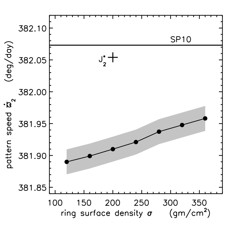
But first note the models’ large discrepancy with the observed free pattern speed reported in SP10, which is the upper horizontal bar in Fig. 6. This discrepancy is not due to the km uncertainty in the ring-edge’s semimajor axis, which makes the simulated ring particles’ mean angular velocity uncertain by the fraction . We find empirically that the simulations’ pattern speeds are also uncertain by this fraction, so deg/day, which is the vertical extent of the gray band around the simulated data in Fig. 6.
Rather, this discrepancy is indirectly due to the absence of the and higher terms from the N-body simulations. To demonstrate this, repeat the gm/cm2 simulation with boosted slightly by factor so that the second zonal harmonic is . This increases the simulated B ring-edge’s angular velocity slightly to deg/day, which is in fact the ring’s true angular velocity at when the higher order and terms are also accounted for33 3 This mean angular velocity is obtained using the physical constants given in the 25 August 2011 Cassini SPICE kernel file: km3/sec2, , , and .. And since Saturn’s gravitational force there is , this means that Saturn’s gravity on the simulated particles at is in fact the true value. Note that boosting to the slightly larger value also requires bringing the simulated Mimas inwards and just interior to its true semimajor axis by 2km. Which speeds up both the forced and free pattern speeds, and is why this simulation’s free pattern speed , which is the cross in Fig. 6, is in better agreement with the observed pattern speed. So the discrepancy between all the other simulated and observed pattern speeds is due to those models’ not accounting for the additional gravity that is due to the and higher terms in Saturn’s oblate figure. Compensating for the absence of those oblateness effects requires altering the simulated satellite’s orbits slightly, which in turn alters the forced and free pattern speeds slightly. But the following will show that these two patterns’ relative speeds are quite insensitive to the particular value of and the absence of the and higher terms.
The best way to compare simulated to observed free patterns is to consider the free pattern speed relative to the forced pattern speed, which is the satellite’s mean angular velocity . That frequency difference is , and is plotted versus ring surface density in Fig. 7. Black dots are from the simulation and the light gray band indicates the deg/day spread that results from the km uncertainty in the ring-edge’s semimajor axis. The relatively large uncertainty in means that one can only conclude from Fig. 7 that gm/cm2. If however the uncertainty in were instead km, then the uncertainty in would be 4 times smaller (darker gray band), which would have allowed us to determine the ring surface density with a much smaller uncertainty of only gm/cm2. The lesson here is that if one wishes to use models of free patterns to infer in, say, narrow ringlets, then one will likely need to know the ring-edge’s semimajor axis with a precision of km.

The cross in Fig. 7 indicates that the the free pattern speed relative to the forced is unchanged when Saturn’s oblateness is boosted to . And to demonstrate that this kind of plot is rather insensitive to oblateness effects, the white dot in Fig. 7 shows that these relative pattern speeds change only very slightly even when is set to zero.
Note though that there will be instances where there is no forced mode with which to compare pattern speeds. In that case it will be convenient to convert the free pattern speed into a radius by solving the Lindblad resonance criterion
| (31) |
for the resonance radius , where is the ring particles’ epicyclic frequency (Eqn. 12b), and at an inner (outer) Lindblad resonance. So for the simulated B ring’s free mode, Eqn. (31) is solved for the radius of the inner Lindblad resonance that is associated with this mode. That quantity is to be compared to a nearby reference distance, which in this case would be the semimajor axis of the B ring’s outer edge . Results are shown in Fig. 8, which shows the simulations’ distance from the B ring’s outer edge to the free pattern’s ILR , , plotted versus ring surface density . Heavier rings have a faster pattern speeds (Fig. 6–7), and so the pattern’s resonance resides at a higher orbital frequency and thus must lie further inwards of the ring’s outer edge in order to satisfy the resonance condition, Eqn. (31). Figure 8 has the same information content as Fig. 7, which is why it also tells us that the B ring’s outer edge has gm/cm2. However a plot like Fig. 8 will also provide the best way to interpret the B ring’s free mode, which is examined below in subsection III.2.
Lastly, note that the free patterns seen in these simulations persist for orbits or 40 years without any sign of damping, despite the ring’s viscosity cm2/sec. This is illustrated in Fig. 9, which plots the ring-edge’s epicyclic amplitude over time for the nominal gm/cm2 simulation. Indeed we have also rerun this simulation using a viscosity that is ten times larger and still saw no damping. These experiments reveal a possibly surprising result, that a free pattern can persist at a ring-edge for a considerable length of time, likely hundreds of years or longer, and Section IV.1 will show that this longevity is due to the viscous forces being several orders or magnitude weaker than the ring’s other interval forces. So one possible interpretation of the free modes seen at the B ring and at other ring edges is that they are relics from past disturbances in Saturn’s ring that may have happened hundreds or more years ago. This possibility is discussed further in Section IV.3.


III.2 the free pattern
The B ring’s free mode has an epicyclic amplitude of km, a pattern speed deg/day, and the inner Lindblad resonance associated with this pattern speed lies km interior to the B ring’s outer edge (SP10).
To excite a free pattern at the ring-edge, place a fictitious satellite in an orbit that has an inner Lindblad resonance km interior to the ring’s outer edge. Noting that the satellite Janus happens to have an resonance in the vicinity, about 2000 km inwards of the B ring’s edge, these simulations use a Janus-mass satellite to perturb the simulated ring for about orbits (about 2 years), which excites an pattern at the ring’s outer edge. The satellite is then removed from the system, which converts the pattern into a free normal mode, and epi_int is then used to evolve the now unperturbed ring for another orbits (about 23 years). Figure 10 plots the ring-edge’s epicyclic amplitude, where it is shown that the free mode persists at the B ring’s outer edge, undamped over time, despite the simulated ring’s viscosity of cm2/sec.
A suite of such B ring simulations is performed, with ring surface densities gm/cm2 and all other parameters identical to the nominal model of Section III.1 except where noted in Fig. 11 caption. The pattern speed of the normal mode is then extracted from each simulation, with those speeds again being slightly faster in the heavier rings. Those pattern speeds are then inserted into Eqn. (31) which is solved for the radius of the inner Lindblad resonance , each of which lies a distance inwards of the ring’s outer edge, and those distances are plotted in Fig. 11 versus ring surface density . The simulated distances are compared to the observed edge-resonance distance reported in SP10, which indicates a ring surface density gm/cm2. This finding is consistent with the the results from the patterns, but this constraint on is again rather loose due to the km uncertainty in the ring-edge’s semimajor axis. But our purpose here is to show how one might use models of free normal modes to infer the surface density of other rings and narrow ringlets, which again will likely require knowing the ring-edge’s semimajor axis to km or better.
Also note that the radial depth of this disturbance is km, about three times smaller than the radial depth of the disturbance.


III.3 the free pattern
The B ring’s free mode has an epicyclic amplitude of km and a pattern speed deg/day that is slightly faster than the local precession rate, and the inner Lindblad resonance that is associated with this pattern speed lies km interior to the B ring’s outer edge (SP10). Several simulations of the B ring’s pattern are evolved for model rings having surface densities of gm/cm2. To excite the pattern at the simulated ring’s edge, again arrange a fictitious satellite’s orbit so that its ILR lies km interior to the B ring’s edge, which is the site where the resonance condition (Eqn. 31) is satisfied when the satellite’s mean angular velocity matches the ring particles’ precession rate, . The simulated ring is perturbed by a satellite whose mass is about 20% that of Mimas, for orbits or 21 years, which excites a forced pattern at the ring’s edge that corotates with the satellite. The satellite is then removed, which converts the forced pattern into a free pattern, and the ring is evolved for another orbits or 83 years. For each simulation the free pattern speed is measured, and Eqn. (31) is then used to convert the free pattern speed into a resonance radius , which is displayed in Fig. 12 that shows that resonance’s distance from the ring’s outer edge, . As the figure shows, the free pattern rotates slightly faster in the heavier ring and thus the associated ILR must lie further inwards in order to satisfy the resonance condition . Again there is no damping of the free pattern, which stays localized at the ring’s outer edge over the simulation’s 83 yr timespan, despite the simulated ring’s viscosity cm2/sec.
The radial depth of this disturbance is much greater than the others, km, which is about four times larger than the disturbance. Comparing Fig. 12 to Figs. 8 and 11 also shows that the LR associated with the disturbance lies about 10 times further from the ring-edge than the and resonances. Which is why the simulation uses streamlines whose width is larger, since a wider portion of the B ring-edge must be simulated in order to capture this disturbances’ deeper reach into the B ring.
Note also that the km uncertainty in this resonance’s position relative to the B ring edge, which is entirely due to the uncertainty in the B ring-edge’s semimajor axis, is in this case relatively small. Which is why the ring’s free mode can also be used to probe its surface density with some precision (unlike the free and modes), and is consistent with a B ring surface density of gm/cm2,

III.4 convergence tests
A number of simulations have also been performed, which repeat the ring simulations using various particle numbers and and various widths of the simulated ring. We find that the results reported here do not change significantly when the simulated ring is populated densely with enough particles, and when the radial width of the simulated B ring is sufficiently wide. Those convergence tests reveal that the number of particles along each streamline must satisfy , that the radial width of each streamline should satisfy , and that the total width of the simulated ring should satisfy . All of the simulations reported here satisfy these requirements.
IV Discussion
This section re-examines the model’s treatment of viscous effects at the ring’s edge, and also describes related topics that will be considered in followup work.
IV.1 the ring’s internal forces
Figure 13 plots the accelerations that the ring’s internal forces—gravity, pressure, and viscosity—exert on each ring particle. These accelerations are from the nominal gm/cm2 simulation that is described in Figs. 5–9, and these accelerations are plotted versus each particle’s distance from the ring’s edge, so those forces obviously get larger closer to the ring’s disturbed outer edge. But the main point of Fig. 13 is that the ring’s self gravity is the dominant internal force in the ring, exceeding the pressure force by a factor of at the ring’s outer edge and by a larger factor elsewhere. Those pressure forces are also about larger than the ring’s viscous forces. But recall that those simulations had zeroed the viscous acceleration that the ring exerts on its outermost streamline (Section III), when that acceleration should instead be as indicated by the large blue dot at the right edge of Fig. 13. Note though that the neglected viscous acceleration of the ring’s edge is still about smaller than that due to ring gravity and smaller than that due to ring pressure. So this justifies neglecting, at least for the short-term yr simulations considered here, the much smaller viscous forces at the ring’s outer edge.
Nonetheless this study’s neglect of the small viscous force at the ring’s outer edge implies that this model does not yet account for the B ring’s radial confinement by Mimas’ ILR. So there appears to be some missing physics that will be necessary if one is interested in the ring’s resonant confinement or the ring’s long-term evolution over yr timescales. The suspected missing physics is described below.

IV.1.1 unmodeled effects: the viscous heating of a resonantly confined ring-edge
The model’s inability to confine the B ring’s outer edge at Mimas’ ILR may be a consequence of the ring’s kinematic viscosity being treated here as a constant parameter everywhere in the simulated ring. Although treating as a constant is a simple and plausible way to model the effects of the ring’s viscous friction, it might not be adequate or accurate if one wishes to simulate the resonant confinement of a planetary ring. This is because the ring’s viscosity transports both energy and angular momentum radially outwards through the ring. So if the ring’s outer edge is to be confined by a satellite’s Lindblad resonance, the satellite must absorb the ring’s outward angular momentum flux, which it can do by exerting a negative gravitational torque at the ring’s edge. But [1] show via a simple Jacobi-integral argument that resonant interactions only allow the satellite to absorb but a fraction of the energy that viscosity delivers to the ring-edge. Consequently the ring’s viscous friction still delivers some orbital energy to the ring-edge where it accumulates and heats up the ring particles’ random velocities . And if collisions among particles are the main source of the ring’s viscosity, then where is the ring’s optical depth [13]. In this case viscous heating would increase as well as at the ring’s edge. The enhanced dissipation there should also increase the angular lag between the ring-edge’s forced pattern and the satellite’s longitude (see Eqn. 83b of Hahn et al. 15). Which will also be important because the gravitational torque that the satellite exerts on the ring-edge varies as [15], and that torque needs to be boosted if the satellite is to confine the spreading ring.
To model this phenomenon properly, the epi_int code also needs to employ an energy equation, one that accounts for how viscous heating tends to increase the ring particles’ dispersion velocity and viscosity nearer the ring’s edge. The increased dissipation and the resulting orbital lag will allow the satellite to exert a greater torque on the ring which, we suspect, will enable the satellite to resonantly confine the simulated ring’s outer edge. The derivation of this energy equation and its implementation in epi_int are ongoing, and those results will be reported on in a followup study.
IV.2 an alternate equation of state
The EOS adopted here is appropriate for a dilute gas of colliding ring particles whose mutual separations greatly exceed their sizes. This should be regarded as a limiting case since ring particles can of course be packed close to each other in the ring. But [4] consider the other extreme limiting case, with close-packed particles that reside shoulder to shoulder in the ring. In that case the ring is expected to behave as an incompressible fluid whose volume density stays constant. So when some perturbation causes ring streamlines to bunch up and increases the ring’s surface density , the ring’s vertical scale height also increases as ring particles are forced to accumulate along the vertical direction. This in turn increases the ring’s pressure due to the larger gravitational force along the vertical direction.
[4] show that infinitesimal density waves in an incompressible disk are unstable and grow in amplitude over time. This phenomenon is related to the viscous overstability, and [21] show that it can distort a narrow eccentric ringlet’s streamlines in a way that accounts for its shapes. [4] also suggest that unstable density waves can be trapped between a Lindblad resonance and the B ring’s outer edge, which might explain the normal modes seen there, and [29] use this concept to estimate the ring’s surface density there.
But keep in mind that this instability only occurs when the ring particles are densely packed to the point of being incompressible, which requires the ring to be very thin and dynamically cold. We have shown here that the amplitude of the B ring’s forced motions indicates that the ring-edge has a surface density gm/cm2. So if this ring is incompressible and composed of icy spheres having a mean volume density of gm/cm3, this then requires a B ring thickness of only meters, which is rather thin compared to other estimates [8]. Similarly the ring particles’ dispersion velocity must be small compared to that expected for a dilute particle gas, so mm/sec), which again is cold compared to all other estimates for Saturn’s rings [8]. The upshot is that an incompressible EOS requires the ring to be very thin and dynamically cold, likely much colder and thinner than is generally thought. Consequently we are optimistic that the compressible EOS used here, , is the appropriate choice for simulations of the outer edge of Saturn’s B ring. Nonetheless in a followup investigation we do intend to encode the incompressible EOS into epi_int, to see if the BGT instability can account for the higher free modes that are seen at the outer edge of the B ring and in many other narrow ringlets.
IV.3 impulse origin for normal modes
The simulations of Section III used a fictitious temporary satellite to excite the free modes that occur at many Saturnian ring edges. These simulations used an admittedly ad hoc method—the sudden appearance and disappearance of a satellite—to excite these modes. Nonetheless these models demonstrate that transient and impulsive events can excite normal modes at ring edges, and those simulations show that normal modes can persist at the ring’s edge for hundreds of years after the disturbance has occurred. Which suggests that an impulsive event in the recent past, perhaps an impact into Saturn’s rings, might be responsible for exciting the normal modes that are seen at the outer edge of the B ring, as well as the normal modes that are also seen along the edges of several narrower ringlets [10, 18, 11, 23]
The possibility that normal modes are due to an impact is motivated by the discovery of vertical corrugations in Saturn’s C and D rings [17, 16] and in Jupiter’s main dust ring [27]. These vertical structures are spirals that span a large swath of each ring, and they are observed to wind up over time due to the central planet’s oblateness. Evolving the vertical corrugations backwards in time also unwinds their spiral pattern until some moment when the affected region is a single tilted plane. Unwinding the Jovian corrugation shows that that disturbance occurred very close to the date when the tidally disrupted comet Shoemaker-Levy 9 impacted Jupiter in 1994, which suggests an impact from a tidally disrupted comet as the origin of these ring-tilts [27]. However a single sub-km comet fragment cannot tilt a large km-wide planetary ring. But a disrupted comet can produce an extended cloud of dust, and if that disrupted dust cloud returns to the planet with enough mass and momentum, then it might tilt a ring that at a later date would be observed as a spiral corrugation.
However the tidal disruption of comet about a low-density planet like Saturn is more problematic, because tidal disruption only occurs when the comet’s orbit is truly close to parabolic and not too hyperbolic, and with periapse just above the planet’s atmosphere [30, 25].
But it is easy to envision an alternate scenario that might be more likely, with a small km-sized comet originally in a heliocentric orbit coming close enough to Saturn to instead strike the main A or B rings. This scenario is more probable because the cross-section available to orbits impacting the main rings is significantly larger than those resulting in tidal disruption. The impacting comet’s considerably greater momentum will nonetheless carry the impactor through the dense A or B rings, but the collision itself is likely energetic enough to shatter the comet. And if that collision is sufficiently dissipative, then the resulting cometary debris will then stay bound to Saturn, and in an orbit that will return that debris back into the ring system on its next orbit. Small differences among the orbits of individual debris particles’ means that, when the debris encounters the rings again, that impacting debris will be spread across a much larger footprint on the ring, which presumably will allow any dense rings or ringlets to absorb the debris’ mass and momentum in a way that effectively gives the ring particles there a sudden velocity kick in proportion to the comet debris density and velocity relative to the ring matter. But if comet Shoemake-Levy 9’s (SL9) impact with Jupiter is any guide, then impact by a cloud of comet debris could last as long week of time, which might tend to smear this effect out due to the ring’s orbital motion. But that effect would be offset if the debris train’s dust cloud is also rather clumpy, like the SL9 debris train was. Indeed, it is possible that this scenario might also account for the spiral corrugations of Saturn’s C and D ring. It is also conceivable that an inclined cloud of impacting comet debris might also excite the vertical analog of normal modes—long-lived vertical oscillations of a ring’s edge. This admittedly speculative scenario will be pursued in a followup study, to determine whether debris from an impact-disrupted comet can excite the normal modes seen at ring edges, and to determine the mass of the progenitor comet that would be needed to account for these modes’ observed amplitudes.
V Summary of results
We have developed a new N-body integrator that calculates the global evolution of a self-gravitating planetary ring as it orbits an oblate planet. The code is called epi_int, and it uses the same kick-drift-step algorithm as is used in other symplectic integrators such as SYMBA and MERCURY. However the velocity kicks that are due to ring gravity are computed via an alternate method that assumes that all particles inhabit a discreet number of streamlines in the ring. The use of streamlines to calculate ring self gravity has been used in analytic studies of rings [12, 2, 5], and the streamline concept is easily implemented in an N-body code. A streamline is the closed path through the ring that is traced by particles having a common semimajor axis. All streamlines are radially close to each other, so the gravitation acceleration due to a streamline is simply that due to a long wire, where is the streamline’s linear density and is the particle’s distance from the streamline. Which is very useful since particles are responding to the pull of smooth wires rather than discreet clumps of ring matter so there is no gravitational scattering. Which means that only a modest number of particles are needed, typically a few thousand, to simulate all of a scalloped ring like the outer edges of Saturn’s A and B ring. Only a few thousand particles are also needed to simulate linear as well as nonlinear spiral density waves, and execution times are just a few hours on a desktop PC.
Another distinction occurs during the particles’ unperturbed drift step when particles follow the epicyclic orbit of [21] about an oblate planet, rather than the usual Keplerian orbit about a spherical planet. This effectively moves the perturbation due to the planet’s oblate figure out of the integrator’s kick step and into the drift step. The code also employs hydrodynamic pressure and viscosity to account for the transport of linear and angular momentum through the ring that arises from collisions among ring particles. Another convenience of the streamline formulation is that it easily accounts for the large pressure drop that occurs at a ring’s sharp edge, as well as the large viscous torque that the ring exerts there. The model also accounts for the mutual gravitational perturbations that the ring and the satellites exert on each other. The epi_int code is written in IDL, and the source code is available for download at http://gemelli.spacescience.org/~hahnjm/software.html.
This integrator is used to simulate the forced response that the satellite Mimas excites at its inner Lindblad resonance (ILR) that lies near the outer edge of Saturn’s B ring. That resonance lies km inwards of the ring’s edge, and simulations show that the ring’s forced epicyclic amplitude varies with the ring’s surface density as . Good agreement with Cassini measurements of occurs when the simulated ring has a surface density of gm/cm2 (see Fig. 5), where the uncertainty in is dominated by the km uncertainty that [29] find in the ring-edge’s semimajor axis. This is the mean surface density over that part of the B ring that is disturbed by this resonance, whose influence in the ring extends to a radial distance of km from the B ring’s outer edge. And if we naively assume that this surface density is the same everywhere across Saturn’s B ring, then its total mass is about of Mimas’ mass.
Cassini observations reveal that the outer edge of Saturn’s B ring also has several free normal modes that are not excited by any known satellite resonances. Although the mechanism that excites these free modes is uncertain, we are nonetheless able to excite free modes in a simulated ring via various ad-hoc methods. For instance, a fictitious satellite’s Lindblad resonance is used to excite a forced pattern at the ring edge. Removing that satellite then converts the forced patten into a free normal mode that persists in these simulations for up to years or orbits without any damping, despite the simulated ring having a kinematic viscosity of cm2/sec; see Fig. 10 for one example.
Alternatively, starting the ring particles in circular orbits while subject to Mimas’ gravitational perturbation excites both a forced and a free pattern that initially null each other precisely at the start of the simulation. But the forced patten corotates with Mimas’ longitude while the free pattern rotates slightly faster in a heavier ring, which suggests that a free mode’s pattern speed can also be used to infer a ring’s surface density . However the free pattern speed is also influenced by the and higher terms in the oblate planet’s gravity field, which are absent from this model which only accounts for the component. So the simulated pattern speed cannot be compared directly to the observed pattern speed; see Fig. 6. To avoid this difficulty, the resonance condition (Eqn. 31) is used to calculate the radius of the Lindblad resonance that is associated with the free normal mode. Plotting the distances of the simulated and observed resonances from the B ring’s edge (Figs. 8, 11, and 12) then provides a convenient way to compare simulations to observations of free modes in a way that is insensitive to the planet’s oblateness.
Simulations of the B ring’s free and patterns are consistent with Cassini measurements of the B ring’s normal modes when the simulated ring-edge again has a surface density of gm/cm2, which is a nice consistency check. But these particular measurements do not provide tight constraint on the ring’s , due to the fact that the and Lindblad resonances only lie km from the outer edge of a ring whose semimajor axis is uncertain by km. However the B ring’s free normal mode does lie much deeper in the ring’s interior, , so the uncertainly in its location is fractionally much smaller, and this normal mode does confirm the gm/cm2 value that was inferred from simulations of the B ring’s forced response .
One of the goals of this study is to determine whether simulations of free modes can be used to determine the surface density and mass of a narrow ringlet. Such ringlets show a broad spectrum of free normal models over [10, 18, 11, 23], and the answer appears to be yes since free pattern speeds do increase with . However Section III.1.2 shows that the semimajor axes of the ringlet’s edges likely need to be known to a precision of km in order for a free mode to provide a useful measurement of the ringlet’s .
The origin of these free modes, which are quite common along the edges of Saturn’s broad rings and its many narrow ringlets, is uncertain. [4] show that, if a planetary ring’s particles are packed shoulder to shoulder such that the ring behaves like an incompressible fluid, then that ring is unstable to the growth of density waves, a phenomenon also termed viscous overstability, and they suggest that the B ring’s normal modes might be due to unstable waves that are trapped between a Lindblad resonance and the ring’s edge. To study this further, we will in a followup study adapt epi_int to employ an incompressible equation of state, to see if the viscous overstability can in fact account for the free normal modes seen along the Saturnian ring edges.
Although the current version of epi_int does not account for the origin of these free modes, one can still plant a free mode along the edge of a simulated ring by temporarily perturbing a ring at a fictitious satellite’s Lindblad resonance, and then removing that satellite, which creates an unforced mode that persists undamped at the ring-edge for more than orbits or yrs despite the simulated ring having a kinematic viscosity of cm2/sec. Because this forcing is suddenly turned on and off, this suggests that any sudden or impulsive disturbance of the ring can excite normal modes, with those disturbances possibly persisting for hundreds or maybe thousands of years. And in Section IV.3 we suggest that the Saturnian normal modes might be excited by an impact with a collisionally disrupted cloud of comet dust. This is a slight variation of the scenario that [17] and [27] propose for the origin of corrugated planetary rings, and in a followup investigation we intend to determine whether such impacts can also account for the normal modes seen in Saturn’s rings.
And lastly, we find that epi_int’s treatment of ring viscosity has difficulty accounting for the radial confinement of the B ring’s outer edge by Mimas’ inner Lindblad resonance. This model employs a kinematic shear viscosity that is everywhere a constant, which causes the simulation’s outermost streamline to slowly but steadily drift radially outwards. Which in turn causes the ring’s forced epicyclic amplitude to slowly grow over time, and makes difficult any comparison to Cassini’s measurement of . To sidestep this difficulty, the model zeros the torque that the simulated ring exerts on its outermost streamline, which does allow the ring to settle into a static configuration that can be compared to Cassini observations and yields a measurement of the ring’s surface density . This approximate treatment is also examined in in Section IV.1, which shows that the viscous acceleration of the ring-edge, had it been included in the simulation, is still orders of magnitude smaller than that due to ring self gravity. So this study of the dynamics of the B ring’s forced and free modes is not adversely impacted by this approximate treatment. But this does mean that the B ring’s radial confinement is still an unsolved problem, and Section IV.1.1 suggests that this might be a consequence of treating as a constant. [1] show that viscosity’s outward transport of energy should also heat the ring’s outer edge and increase the ring particles’ dispersion velocity there. And if collisions among ring particles are the dominant source of ring viscosity, then and viscous dissipation would be enhanced at the ring edge, which in turn would increase the angular lag between the ring’s forced response and the Mimas’ longitude. That then would increase the gravitational torque that that satellite exerts on the ring-edge. So in a followup study we will modify epi_int to address this problem in a fully self-consistent way, to see if enhanced dissipation at the ring-edge also increases Mimas’ gravitational torque there sufficiently to prevent the B ring’s outer edge from flowing viscously beyond that satellite’s inner Lindblad resonance.
Appendix A Appendix A
The following calculates the flux of angular momentum that is communicated via a disk’s viscosity. The disk is flat and thin and has a vertical halfwidth and constant volume density that is related to its surface density via . The disk is assumed viscous, and its gravity is ignored here since this Appendix is only interested in the angular momentum flux that is transported solely by viscosity.
The density of angular momentum in the disk is , and the vertical component along the axis is in Cartesian coordinates and where and are functions of position and time, so the time rate of change of is
| (A1) |
The time derivatives in the above are Euler’s equation,
| (A2) |
where the are the elements of the momentum flux density tensor
| (A3) |
where is the pressure and are the elements of the viscous stress tensor [20]. Inserting Eqn. (A3) into (A1) yields
| (A4) |
where the vector
| (A5) |
is the flux density of the component of linear momentum and is the unit vector along the axis. Equation (A4) can be rewritten
| (A6) |
but note that since the viscous stress tensor is symmetric (Eqn. A11), so
| (A7) |
where
| (A8) |
Integrating Eqn. (A7) over some volume that is bounded by area yields
| (A9) |
by the divergence theorem, so Eqn. (A9) indicates that is the flux of the component of angular momentum out of volume that is being transported by advection, pressure, and viscous effects.
This Appendix is interested in the part of that is due to viscous effects, which will be identified as and is obtained by replacing in Eqn. (A3) with so
| (A10) |
This is the 2D flux of the component of angular momentum that is transported by the disk’s viscosity whose horizontal components in Cartesian coordinates are where and . However this Appendix desires the radial component of are some site in the disk, which is .
The elements of the viscous stress tensor are [20]
| (A11) |
where is the shear viscosity, is the bulk viscosity, and is the Kronecker delta. Inserting this into and replacing and then yields
| (A12) |
The horizontal velocities are and when written in terms of their radial component and tangential component . The derivatives in Eqn. (A12) are
| (A13) |
when written in terms of cylindrical coordinates, and the combinations of derivatives in Eqn. (A12) are
| (A14a) | |||||
| (A14b) | |||||
Inserting these into Eqn. (A12) then yields a result that is thankfully much more compact,
| (A15) |
noting that the second term in Eqn. (A15) may be neglected since the azimuthal gradient is much smaller than the radial gradient for the disks considered here. This is the radial component of the disk’s 2D viscous angular momentum flux density, so the 1D viscous angular momentum flux density is Eqn. (A15) integrated through the disk’s vertical cross section:
| (A16) |
where is the disk’s kinematic shear viscosity.
Appendix B Appendix B
The flux density of -type momentum is (see Eqn. A5) while the flux density of -type momentum is , so the flux density of radial momentum is and the radial component of this momentum flux density is
| (B1) | |||||
| (B2) |
where is the unit vector in the radial direction. The part of that momentum flux that is transported solely by viscous effects will be called and is again obtained by replacing the in the above with :
| (B3) | |||||
| (B4) |
Equations (A13) provide the combination
| (B5) |
and inserting this plus Eqn. (A14a) into Eqn. (B3) then yields
| (B6) |
but the term is again neglected in the streamline approximation. This is the 2D radial momentum flux due to viscous transport, so the vertically integrated linear momentum flux due to viscosity is
| (B7) |
References
- [1] Borderies, N., Goldreich, P., & Tremaine, S. 1982, Nature, 299, 209
- [2] —. 1983a, AJ, 88, 1074
- [3] —. 1983b, Icarus, 55, 124
- [4] —. 1985, Icarus, 63, 406
- [5] —. 1986, Icarus, 68, 522
- [6] Borderies-Rappaport, N. & Longaretti, P.-Y. 1994, Icarus, 107, 129
- [7] Chambers, J. E. 1999, MNRAS, 304, 793
- [8] Cuzzi, J. N., Burns, J. A., Charnoz, S., Clark, R. N., Colwell, J. E., Dones, L., Esposito, L. W., Filacchione, G., French, R. G., Hedman, M. M., Kempf, S., Marouf, E. A., Murray, C. D., Nicholson, P. D., Porco, C. C., Schmidt, J., Showalter, M. R., Spilker, L. J., Spitale, J. N., Srama, R., Sremčević, M., Tiscareno, M. S., & Weiss, J. 2010, Science, 327, 1470
- [9] Duncan, M. J., Levison, H. F., & Lee, M. H. 1998, AJ, 116, 2067
- [10] French, R. G., Marouf, E. A., Rappaport, N. J., & McGhee, C. A. 2010, AJ, 139, 1649
- [11] French, R. G., Nicholson, P. D., Colwell, J., Marouf, E. A., Rappaport, N. J., Hedman, M., Lonergan, K., McGhee-French, C., & Sepersky, T. 2011, in EPSC-DPS Joint Meeting 2011, 624
- [12] Goldreich, P. & Tremaine, S. 1979, AJ, 84, 1638
- [13] —. 1982, ARA&A, 20, 249
- [14] Goldstein, H. 1980, Classical mechanics (2nd ed.) (Reading, Massachusetts:Addison-Wesley)
- [15] Hahn, J. M., Spitale, J. N., & Porco, C. C. 2009, ApJ, 699, 686
- [16] Hedman, M. M., Burns, J. A., Evans, M. W., Tiscareno, M. S., & Porco, C. C. 2011, Science, 332, 708
- [17] Hedman, M. M., Burns, J. A., Showalter, M. R., Porco, C. C., Nicholson, P. D., Bosh, A. S., Tiscareno, M. S., Brown, R. H., Buratti, B. J., Baines, K. H., & Clark, R. 2007, Icarus, 188, 89
- [18] Hedman, M. M., Nicholson, P. D., Baines, K. H., Buratti, B. J., Sotin, C., Clark, R. N., Brown, R. H., French, R. G., & Marouf, E. A. 2010, AJ, 139, 228
- [19] Kudryavtsev, L. D. & Samarin, M. K. 2013, Lagrange interpolation formula, Encyclopedia of Mathematics. URL: http://www.encyclopediaofmath.org/index.php? title=Lagrange interpolation formula&oldid=17497
- [20] Landau, L. D. & Lifshitz, E. M. 1987, Fluid mechanics, 2nd Ed. (Elsevier)
- [21] Longaretti, P.-Y. & Rappaport, N. 1995, Icarus, 116, 376
- [22] Melita, M. D. & Papaloizou, J. C. B. 2005, Celestial Mechanics and Dynamical Astronomy, 91, 151
- [23] Nicholson, P. D., French, R. G., & M., H. M. 2012, contributed talk at AAS/DDA conference, 1, 1
- [24] Pringle, J. E. 1981, ARA&A, 19, 137
- [25] Richardson, D. C., Bottke, W. F., & Love, S. G. 1998, Icarus, 134, 47
- [26] Salo, H. 1995, Icarus, 117, 287
- [27] Showalter, M. R., Hedman, M. M., & Burns, J. A. 2011, Science, 332, 711
- [28] Shu, F. H. 1984, in IAU Colloq. 75: Planetary Rings, ed. R. Greenberg & A. Brahic, 513–561
- [29] Spitale, J. N. & Porco, C. C. 2010, AJ, 140, 1747
- [30] Sridhar, S. & Tremaine, S. 1992, Icarus, 95, 86
- [31] Tiscareno, M. S., Burns, J. A., Nicholson, P. D., Hedman, M. M., & Porco, C. C. 2007, Icarus, 189, 14
- [32] Ward, W. R. 1986, Icarus, 67, 164