Quantum entanglement entropy and classical mutual information in long-range harmonic oscillators

A useful method to obtain entanglement entropy is introduced in [7] and rediscovered in [8] and generalized to Rényi entropy in [9]. In this method one would like to measure the quantum entanglement entropy of the ground state of the free field $\{\phi\}$, generated by tracing over fields inside of the region of the boundary surface. To fix the notation and for the later use we give here a brief summary of the work described in more detail in the Ref. [7, 9]. The ground state wave functional is given by

$$\Psi_{0}(\{\phi\})\propto(\text{det}\Gamma)^{\frac{1}{4}}\exp\{-\sum_{n,n^{\prime}=1}^{N}\phi_{n}\Gamma_{nn^{\prime}}\phi_{n^{\prime}}\}.$$

(12)

where $\{\phi\}$ denotes the collection of all $\phi$’s, one for each oscillator and $\Gamma=K^{1/2}$.

Now consider a subregion in the total space and split the field variables into “inside” ($\{\phi\}_{A}$) and “outside” ($\{\phi\}_{B}$) parts, then one can rewrite the ground state wave function as

$\displaystyle\Psi_{0}\propto\exp\{-(\{\phi\}_{A}~\{\phi\}_{B})\begin{pmatrix}\Gamma_{AA}&\Gamma_{AB}\\ \Gamma_{BA}&\Gamma_{BB}\end{pmatrix}\begin{pmatrix}\{\phi\}_{A}\\ \{\phi\}_{B}\end{pmatrix}\}~,$

(13)

where $\Gamma_{\oplus\otimes}$ ($\oplus=\{A,B\}$ and $\otimes=\{A,B\}$) denotes the kernel matrix restricted to the inside or the outside.

For the fields $\{\phi^{1,2}\}_{A}$ which are defined in the inside region, the ground state density matrix $\rho_{A}(\{\phi^{1}\}_{A},\{\phi^{2}\}_{A})$, is given by

$\displaystyle\begin{split}\rho_{A}(\{\phi^{1}\}_{A};\{\phi^{2}\}_{A})&\propto(\text{det}(\Gamma_{AA})^{-1})^{\frac{1}{2}}\exp\{-{1\over 2}\times\\ &(\{\phi^{1}\}_{A}~\{\phi^{2}\}_{A})\begin{pmatrix}\mathcal{A}&2\mathcal{B}\\ 2\mathcal{B}&\mathcal{A}\end{pmatrix}\begin{pmatrix}\{\phi^{1}\}_{A}\\ \{\phi^{2}\}_{A}\end{pmatrix}\}~,\end{split}$

(14)

where

	$\displaystyle\mathcal{A}$	$\displaystyle=$	$\displaystyle 2(\Gamma_{AA}-{1\over 2}\Gamma_{AB}(\Gamma_{BB})^{-1}\Gamma_{BA});$		(15)
	$\displaystyle\mathcal{B}$	$\displaystyle=$	$\displaystyle-{1\over 2}\Gamma_{AB}(\Gamma_{BB})^{-1}\Gamma_{BA}~.$		(16)

From now on one can follow two different methods to get the entanglement entropy: one is based on direct diagonalization of the above reduced density matrix and the other based on using replica trick. For later use we will summarize the results for both of them. Using appropriate transformations [7] one can write the reduced density matrix as

$\displaystyle\begin{split}&\rho_{A}(\{\phi^{1}\}_{A};\{\phi^{2}\}_{A})=\prod_{i}\frac{1}{\sqrt{\pi}}\times\\ &\exp\{-\frac{1}{2}(\phi_{n}^{1}\phi^{1n}+\phi_{n}^{2}\phi^{2n})-\frac{1}{4}E_{i}(\phi^{1}-\phi^{2})_{n}(\phi^{1}-\phi^{2})^{n}\}\end{split}$

(17)

where $E_{i}$’s are the eigenvalues of the matrix $\Lambda$ with the following simple form

$$\Lambda\equiv-(\Gamma^{-1})_{AB}~\Gamma_{BA}~.$$

(18)

The interesting point about the equation (17) is that it has the form of the reduced density matrix of two body harmonic oscillator. In other words for the ground state of coupled harmonic oscillator the problem of calculating the entanglement entropy can be reduced to the problem of calculating the entanglement entropy of two coupled harmonic oscillators. One can then show that the entropy can be expressed in terms of the eigenvalues $E_{i}$ of $\Lambda$ as [7]:

$$S=\sum_{i}\left[\log\frac{\sqrt{E_{i}}}{2}+\sqrt{1+E_{i}}\log(\frac{1}{\sqrt{E_{i}}}+\sqrt{1+\frac{1}{E_{i}}})\right]~.$$

(19)

It is worth mentioning that having larger coupling between two oscillators leads to larger $E$ and consequently larger entanglement entropy.

The second method which is also useful to get the Rényi entropy is based on Replica trick. Using Eq. (14), and rescaling the reduced density matrix one can calculate ${\rm\tr}\rho_{A}^{n}$ and ultimatley the entropy [9] as following sum

$$S=\lim_{n\rightarrow 1}\frac{1}{1-n}\log(\rm\tr\rho_{A}^{n})=-\sum_{i=1}^{l}\{{\rm ln}(1-\xi_{i})+{\xi_{i}\over 1-\xi_{i}}{\rm ln}\xi_{i}\}~,$$

(20)

where $\xi_{i}$ is related to the eigenvalue of the matrix $\mathcal{C}=-2\mathcal{A}^{-1}\mathcal{B}$ by $\mathcal{C}_{i}=\frac{2\xi_{i}}{1+\xi_{i}^{2}}$ .

It is also useful to consider the matrix $\Lambda=(1-\mathcal{P})^{-1}\mathcal{P}$ where $\mathcal{P}\equiv\Gamma_{AA}^{-1}\Gamma_{AB}\Gamma_{BB}^{-1}\Gamma_{BA}$ which has also the simple form (18) and write Eq. (20) in terms of eigenvalues of the matrix $\Lambda$ as (19). The eigenvalues $E_{i}$ of the matrix $\Lambda$ are positive and related to $\xi_{i}$ by

$$\xi_{i}=\frac{\sqrt{1+E_{i}}-1}{\sqrt{1+E_{i}}+1}~.$$

(21)

It is also straightforward to write the Rényi entropy $S_{n}$ in term of $\xi_{i}$ as:

$\displaystyle S_{n}=\frac{1}{n-1}\sum_{i}\left(\log(1-\xi_{i}^{n})-n\log(1-\xi_{i})\right)~.$

(22)

In order to compute the entanglement entropy obtained by tracing over the fields in the region $A$ for a given problem, one should find the eigenvalues of the matrix $\Lambda$. For a given hamiltonian $\mathcal{H}$ one can easily find the operators $K$ and consequently $\Gamma$ and $\Gamma^{-1}$. In the continuum limit, the operator $\Lambda$ is obtained after integration over the oscillators in the region $B$ as

$$\Lambda(x,y)=-\int_{B}dz\Gamma^{-1}(x,z)\Gamma(z,y).$$

(23)

The eigenvalue problem to be solved is then

$$\int dy\Lambda(x,y)\psi(y)=E\psi(x),$$

(24)

where $\psi(x)$ is an eigenfunction with eigenvalue $E$.

It is worth mentioning that for the general Hamiltonian Eq. (1), one can calculate the two point correlators $X_{A}=\rm\tr(\rho_{A}\phi_{i}\phi_{j})$ and $P_{A}=\rm\tr(\rho_{A}\pi_{i}\pi_{j})$ using the $K$ matrix by

$\displaystyle\frac{1}{2}K^{-1/2}=\begin{pmatrix}X_{A}&X_{AB}\\ X^{T}_{AB}&X_{B}\end{pmatrix},\hskip 5.69046pt\frac{1}{2}K^{1/2}=\begin{pmatrix}P_{A}&P_{AB}\\ P^{T}_{AB}&P_{B}\end{pmatrix}~,$

(25)

Then one can define matrix $C=\sqrt{X_{A}P_{A}}$, which has the eigenvalues [5],

$$\nu_{i}=\coth(-\log(\frac{\sqrt{1+E_{i}}-1}{\sqrt{1+E_{i}}+1})/2),$$

(26)

where $\nu_{i}$ are the eigenvalues of $C$. With respect to the new operators the entropy is given by

	$\displaystyle S$	$\displaystyle=\rm\tr\left[(C+\frac{1}{2})\log(C+\frac{1}{2})-(C-\frac{1}{2})\log(C-\frac{1}{2})\right]$			(27)
		$\displaystyle=\sum_{i=1}^{l}\left[(\nu_{i}+\frac{1}{2})\log(\nu_{i}+\frac{1}{2})-(\nu_{i}-\frac{1}{2})\log(\nu_{i}-\frac{1}{2})\right]~.$

We also have

	$\displaystyle S_{n}$	$\displaystyle=$	$\displaystyle\frac{1}{n-1}\rm\tr\left[\log\left((C+\frac{1}{2})^{n}-(C-\frac{1}{2})^{n}\right)\right]$		(28)
		$\displaystyle=$	$\displaystyle\frac{1}{n-1}\sum_{i=1}^{l}\left[\log\left((\nu_{i}+\frac{1}{2})^{n}-(\nu_{i}-\frac{1}{2})^{n}\right)\right],$

where $l$ is the size of the subsystem $A$. In this formulation we need only the correlators inside the region $A$, to calculate $S$ and $S_{n}$.

In order to clarify the hamiltonian approach in the continuum limit, we briefly review the procedure followed in [9] to find an approximate analytical solution for the harmonic oscillator system with short-range interaction. This method is introduced in order to determine $E$ and also $S$ by using eigenvalue problem Eq. (24). They considered a one dimensional coupled harmonic oscillator with mass $M$, confined to the region $-L<x<L$ and the subsystem is taken to be half of a finite system.

To calculate the eigenvalue $E$, for system of harmonic oscillators with short-range interactions, it is better to first consider a system with infinite size $L\rightarrow\infty$. At this limit the kernels $\Gamma^{\pm 1}$ needed to construct $E$ have the following forms:

$\displaystyle\begin{split}&\Gamma(x,y)=MK_{1}(M(x-y))/(\pi(x-y))~,\\ &\Gamma^{-1}(x,y)=K_{0}(M(x-y))/\pi~.\end{split}$

(29)

where $M$ is the mass term. In the $M\rightarrow 0$ limit it is easy to show that $\psi=\exp(\imath\omega\ln x)$ is an eigensolution of the Eq. (24) with eigenvalue

$$E={\rm sinh}^{-2}(\pi\omega)~.$$

(30)

To discretize the spectrum and calculate the entropy, one needs to impose Dirichlet boundary conditions at some large $x=L$ and further Dirichlet condition at some small $x=\epsilon$. The eigenvalues and eigenvectors are then:

$$\psi(x)=\sin(\omega(E)\ln(x/\epsilon)),\hskip 5.69046pt\omega(E_{i})\ln(L/\epsilon)=\pi i~.$$

(31)

It is useful to note that the density of states per unit $\omega$ interval is constant. Now one can rewrite the continuum limit of the Rényi entropy Eq. (22) and the entanglement entropy as an integral over $\omega$,

$$S_{n}=\frac{\log L}{\pi(n-1)}\int_{0}^{\infty}d\omega(\log(1-\xi^{n})-n\log(1-\xi)),$$

(32)

$$S=\frac{\log L}{\pi}\int_{0}^{\infty}d\omega\left(\frac{\xi}{\xi-1}\log(\xi)-\log(1-\xi)\right),$$

(33)

where $\xi(\omega)$ is defined in the Eq. (21).

As discussed before, conformal invariance implies universal properties for the entanglement entropy. The entanglement entropy and also the Réyni entropy for these models, diverge logarithmically with the subsystem size with prefactors proportional to $c$ and $c_{n}$, respectively.

By using the Eq. (33) and also Eqs. (21) and (30) one can find the entanglement entropy $S$ for the harmonic oscillator problem, giving the result $S=\frac{1}{6}\log(L/\epsilon)$ which is consistent with $c=1$. In addition using (32) one can also find the Rényi entropy $S_{n}=\frac{1}{12}\left(1+\frac{1}{n}\right)\ln(L/\epsilon)$ consistent with the CFT predictions [31].

Next we consider short-range harmonic oscillator with infinite size and sub-system with length $l$. This kind of configuration is completely different from the Ref. [9]. We should remember that the Eqs. (30) and (31) are no longer true in this configuration. We proceed with the Eq. (23). To evaluate this integral we must consider $B\in\left(-\infty<z<0\right)\cup\left(l<z<\infty\right)$ as the complement of the sub-region $l$. The matrix $\Lambda$ becomes:

	$\displaystyle\Lambda(x,y)$	$\displaystyle=$	$\displaystyle-\frac{1}{\pi^{2}}\int_{B}\frac{\ln(x+z)}{(z+y)^{2}}dz$		(34)
		$\displaystyle=$	$\displaystyle\frac{1}{\pi^{2}}\bigg\{\frac{\left(l-x\right)\log(l-x)-\left(l-y\right)\log(l-y)}{(l-y)(y-x)}$
		$\displaystyle-$	$\displaystyle\frac{x\log(x)-y\log(y)}{(y-x)y}\bigg\}.$

Therefore, according to Eq. (24), the eigenvalues $E_{i}$ and the corresponding eigenfunctions $\psi_{i}(x)$ can be obtained by diagonalizing $\Lambda$ matrix. Unfortunately we were unable to find $E_{i}$ analytically. One can numerically evaluate $E_{i}$ and $\psi_{i}$ using direct diagonalization of the matrix $\Lambda$, then try to guess the formula for eigenvalues and eigenfunctions. We shall come to this problem in the next section by means of numerical calculations.

We are now ready to speak more about the LRHO with $\alpha<2$. To determine $E$ and $\psi$ for LRHO, we calculated first the matrices $\Gamma=K^{1/2}$ and $\Gamma^{-1}=K^{-1/2}$. The continuum limit of the matrices $\Gamma$ and $\Gamma^{-1}$ has the following forms:

$\displaystyle\begin{split}\Gamma^{\pm 1}(x,y)&=\frac{1}{2\pi}\int_{-\infty}^{\infty}dk(|k|^{\alpha}+M^{\alpha})^{\pm 1/2}e^{ik.(x-y)}\\ &=\frac{1}{2\Gamma[\mp\alpha/2]}\frac{1}{|r|^{1\pm\alpha/2}}\times\\ &H_{3,2}^{1,2}\left(\left(M|r|\right)^{\alpha}\middle|\begin{array}[]{c}(1,1)(\mp\frac{\alpha}{2},1)(\mp\frac{\alpha}{4},\frac{\alpha}{2})\\ (\mp\frac{\alpha}{2},1)(\mp\frac{\alpha}{4},\frac{\alpha}{2})\end{array}\right)\\ &=\frac{1}{2\Gamma[\mp\alpha/2]\cos(\frac{\pi\alpha}{4})}\frac{1}{|r|^{1\pm\alpha/2}}+\mathcal{O}(M^{\alpha})~,\end{split}$

(35)

where $r=x-y$ and $H_{3,2}^{1,2}$ is the Fox H-Function. Then in a similar way as in Eq. (23), we found the matrix $\Lambda$ by multiplying $\Gamma$ and $\Gamma^{-1}$ in the complement region $B\in\left(-\infty<z<0\right)\cup\left(l<z<\infty\right)$ as

$\displaystyle\Lambda(x,y)=\mathfrak{A}\left[\frac{2\left(\left(\frac{l-x}{l-y}\right)^{\alpha/2}-\left(\frac{x}{y}\right)^{\alpha/2}\right)}{\alpha(x-y)}\right]\hskip 2.84544pt(\alpha<2)$

(36)

where $\mathfrak{A}=\frac{1}{4\Gamma[-\alpha/2]\Gamma[\alpha/2]\cos^{2}(\frac{\pi\alpha}{4})}$. Unfortunately, the exact solution of the eigenvalues and the corresponding eigenfunctions for Eq. (36) are not known and remain an open problem. It is nonetheless both possible and interesting to investigate the properties of the $E$ and $\psi$, for LRHO problem, numerically. In the next section we will discuss our numerical findings.

It is worth mentioning that, the Eq. (36) is only true for an infinitely large system compared to the sub-system size. However one can also study LRHO problem in the presence of boundary but since boundary of the finite system breaks the translational invariance, we have not been able to find $\Gamma^{\pm 1}$ explicitly because we are not allowed to use Fourier transform for the finite systems. Therefore we studied this case just numerically, which we will present the results in the next sections.

As explained above, we can find the eigenvalues $E$ and the corresponding eigenvectors $\psi(x)$ for a given matrix $K$, and we can also study the scaling behaviors of the entanglement entropy $S$ and the Rényi entropy $S_{n}$.

In the next section we will speak more about our results but here we will discuss about different configurations for the system and also subsystem that we have used in our study. In this work we consider five main kinds of configurations depicted in Fig. (1) for system and subsystem. In the massless case:

• $\mathfrak{C_{1}}$:

  System is very large and $A$ is a small sub-system with length $l$.

• $\mathfrak{C_{2}}$:

  System with periodic boundary condition has finite size $L$, and $A$ is a sub-system with length $l$.

• $\mathfrak{C_{3}}$:

  System with size $L$ has boundary and is divided to two adjacent parts. The first part is a sub-system with length $l<L$ and the second part is the complement with size $L-l$.

• $\mathfrak{C_{4}}$:

  System with size $2L$ has boundary and is divided to two adjacent equal intervals with length $l=L$ where one of them is the sub-system.

In the massive case:

• $\mathfrak{C_{5}}$:

  System is very large and $A$ is a sub-system with length $l$.

We now numerically evaluate the von Neumann entanglement entropy $S$ and the Rényi entropy $S_{n}$ for LRHO problem in different cases ($\mathfrak{C_{i}}$,$i=1\dots 5$), by using Eqs. (19) and (22) or equivalently Eqs. (27) and (28), which was first studied in [24]. In this respect, we follow the method explained in the last section. We will measure the eigenvalues $E_{i}$ and the eigenfunctions $\psi_{i}(x)$ in Eq. (24) numerically and then we introduce an expression for $E$ and $\psi$, which matches to the numerical simulations. Our motivation to study these quantities with full detail is related to our interest in better understanding the operator (36) which its eigenvalues provide the entanglement entropy. We should here stress that we calculate the entanglement entropy using the numerical $\Lambda$ matrix and not by discretizing the operator (36). However we will confirm that these two operators are very close to each other if we consider large systems and consequently can approximate each other.

In order to calculate $E$ and $\psi$, we first need to construct the matrix $\Lambda$ for a given $K$ matrix. Numerically one can find the matrix $\Lambda\equiv-\Gamma^{-1}_{+-}\Gamma_{-+}$ by multiplying $\Gamma^{-1}$ and $\Gamma$, where $\Gamma=K^{1/2}$ and $\Gamma^{-1}=K^{-1/2}$. For example we applied this method to the LRHO with very large system size and small sub-region $l$. There is a very good agreement between numerical $\Lambda$ and the matrix $\Lambda(x,y)$ coming from Eqs. (34) and (36), when the distances are more than four lattice sizes.

To obtain a better understanding of the long-range harmonic oscillator problem, we studied first the eigenvalues $E_{i}$ and the eigenfunctions $\psi_{i}$ of the short-range harmonic oscillator. We considered a system with size $2L$ and the subsystem is taken to be half of the system size ($\mathfrak{C_{4}}$). Then using the numerical methods, we diagonalized the matrix $\Lambda$ to find $E_{i}$ and $\psi_{i}$. In Fig. (2) we sketched logarithm of the eigenvalues $E_{i}$ with respect to $\omega(E_{i})$. As can be seen, the result obtained from Eq. (30) has similar asymptotic behavior as numerical simulations. In addition the eigenvectors $\psi(x)$ for the first and second largest eigenvalues, $E_{1}$ and $E_{2}$ verify the behavior predicted in Eq. (31). We have also calculated the prefactor $c$ numerically and our result is consistent with the theoretical prediction. The numerical results of entanglement entropy for LRHO ($\alpha<2$) for the systems with boundary e.g. $\mathfrak{C_{3}}$ and $\mathfrak{C_{4}}$, are summarized in the next sections.

Next we discuss the case, where the subsystem is very small with length $l$ and the system is very large ($\mathfrak{C_{1}}$). For this configuration, as a first step, we have studied the properties of $E_{i}$ and $\psi_{i}$ for harmonic oscillator problem with short-range interaction by a direct diagonalization of the matrix $\Lambda$. Numerical results are shown in Fig. (3). It is interesting to note that, when we choose $\omega(E_{i})=\pi i/2(\log(l)+\zeta)$ ($\zeta=1.3$), apart from a constant, which it appears ubiquitously in this kind of studies [10], the behavior of the eigenvalues $E_{i}$ are in very good agreement with $E(\omega)=1/\sinh^{2}(\pi\omega)$ (see Fig . (2)). Let us remark that $\omega(E)$ for the configuration $\mathfrak{C_{1}}$, differs from Ref. [9] by a factor two and a constant $\zeta$. We studied the scaling of $S$ versus the logarithm of the sub-system size, $\log l$, and compared with Eq. (10). Our result agrees with $c=1$.

The next step is to analyze the eigenvalues $E$ of the Eq. (36) for LRHO with $\alpha<2$. As we remarked before, if we consider very small sub-region of LRHO with $\alpha=2$ and very large system size ($\mathfrak{C_{1}}$), we expect $E_{i}\sim\sinh^{-2}(\pi\omega_{i})$ and $\omega(E_{i})=i\pi/2(\log(l)+\zeta)$. For other values of $\alpha$, the eigenvalues behavior can be seen in the Fig. (4), where we compared $\log(E)$ vs. $\omega$ for various $\alpha$’s. Let us first address the behavior of small eigenvalues $E_{i}$ (large $i$, i.e. $i>3$). Our results show that the small eigenvalues are independent of $\alpha$ and $\log(E_{i})$ is linearly dependent to $\omega_{i}$ by scaling factor $-2\pi$. Then one can get the asymptotic behavior $E_{i}\propto e^{-2\pi\omega_{i}}$ for $i>3$ and from our previous knowledge about $E_{i}$ for $\alpha=2$, one can conjecture the simple behavior $E_{i}\propto\sinh^{-2}(\pi\omega_{i})$. In our numerical simulations we used $\omega_{i}=i\pi/2(\log(l)+\zeta)$, where $\zeta$ is a $\alpha$ dependent parameter ( $\zeta\in\left[1.0,2.0\right]$), to get the best fit to numerical data. We may use this behavior and guess the asymptotic expression for the eigenvalue $E$ as

$\displaystyle E(\omega)=\frac{a(\alpha)}{\sinh^{2}(\pi\omega)+b(\alpha)}.$

(37)

The best fit parameters to our numerical data were $a(\alpha)=\frac{\alpha}{2}\sin^{2}(\frac{\pi\alpha}{4})$ and $b(\alpha)=0.12\alpha+0.19\alpha^{2}-0.20\alpha^{3}+0.04\alpha^{4}$ . The value of $b(\alpha)$ is zero at $\alpha=0$ and $\alpha=2$ and it has a maximum at $\alpha=1$.

Next, we studied the eigenvector $\psi_{i}(x)$ of the matrix $\Lambda$ for LRHO numerically. By diagonalizing $\Lambda$ we can also find the eigenvalues $E_{i}$. The eigenvector $\psi_{i}$ can then be computed for each $E_{i}$ by $\Lambda\psi_{i}=E_{i}\psi_{i}$. A typical example is shown in Fig. (5), where one can see that the eigenfunctions $\psi_{i}(x)$ are symmetric around $x=l/2$ for odd $i$, and antisymmetric for even $i$. We found that the best fit to the eigenvectors $\psi_{i}(x)$ is

	$\displaystyle\psi_{i}(x)$	$\displaystyle=$	$\displaystyle\frac{1}{\mathcal{N}}\{\left(x^{\imath\omega_{i}+b}+x^{-\imath\omega_{i}+b}\right)$		(38)
		$\displaystyle-$	$\displaystyle(-1)^{i}\left((l-x)^{\imath\omega_{i}+b}+(l-x)^{-\imath\omega_{i}+b}\right)\};$

where $\mathcal{N}$ is the normalization coefficient and $b\in\left[-1,0\right]$ is the free parameter to get the best fit to the numerical data. In Eq. (38) we used $\omega_{i}=\frac{i\pi}{2(\log l+\zeta)}$. The values of the free parameters $b$ and $\zeta$ in general depend on $\alpha$. In Fig. (5) the behavior of the $\psi$ for LRHO problem with $\alpha=1$ and also the best fit to the Eq. (38), are shown, as a function of $x$.

As argued before, we studied the eigenvalue problem Eq. (24) for LRHO, in order to find the eigenfunction $\psi_{i}(x)$ and corresponding eigenvalue $E_{i}$. The von Neumann entanglement entropy $S$ and the Rényi entropy $S_{n}$ can be obtained as functions of $E$ (see Eq. (22)). It is possible to find $S$ and also $S_{n}$ using Eq. (27 ) and Eq. (28), respectively.

Finally, we discuss the goodness of Eq. (37). For arbitrary values of the long-range interaction $\alpha$, the von Neumann entanglement entropy $S$ and the Rényi entropy $S_{n}$ can in practice be obtained by $(i)$ evaluating Eq. (2) numerically for system with total size $L$ and compute $X_{A}$ and $P_{A}$ from $K$ matrix (see Eq. (25)), $(ii)$ diagonalizing $C$ to obtain $\nu_{i}$, and $(iii)$ evaluating (27) and (28), where $l$ is the number of lattice sites in the subsystem $A$.

We observe that, in the LRHO problem the entanglement entropy and the Rényi entropy increase logarithmically with the sub-system size as

$$S\sim\frac{\tilde{c}(\alpha)}{3}\log l~,$$

(39)

and

$$S_{n}\sim\frac{\tilde{c}_{n}(\alpha)}{3}\log l~,$$

(40)

respectively. By studying the scaling behavior of $S$ and also $S_{n}$ vs. $\log l$, one can find the scaling parameters $\tilde{c}(\alpha)$ and $\tilde{c}_{n}(\alpha)$. We display the resulting quantities for different values of $\alpha$ and $n$, in Fig. (6).

For arbitrary values of $\alpha$ and $n$, according to Eqs. (32) and (33) and also Eq. (37), one can find the prefactors $\tilde{c}(\alpha)$ and $\tilde{c}_{n}(\alpha)$. We have depicted the results coming from these formulas in Fig. (6), and we found perfect agreement between our results, confirming the validity of the Eq. (37).

There are some comments in order: the fact that the coefficient of the logarithm is an increasing function of $\alpha$ is somehow counter intuitive because we know that for bigger $\alpha$’s the interaction get weaker by the distance faster than the smaller $\alpha$’s. There are some ways to roughly understand this result: from mathematical point of view one might argue that the entanglement entropy is actually related to the eigenvalues of the matrix $\Lambda$ and those eigenvalues are smaller when we take smaller $\alpha$’s. This can be seen easily by looking to the equation (36). These eigenvalues are also the parameters that appear after mapping the many body harmonic oscillator to the two body case in equation (17). Stronger couplings between two oscillators leads to bigger $E$ and consequently bigger entanglement among them. The fact that after diagonalization we have smaller $E_{i}$’s for smaller $\alpha$’s shows that although the interactions between oscillators far from each other is much stronger for smaller $\alpha$’s, that still does not guaranty bigger entanglement entropy. One might understand this phenomena as follows: based on the equation (2) in the range $0<\alpha<2$ one can see that $K(1)$, which is related to the nearest neighbor interaction, is an increasing function with respect to $\alpha$ but $K(n)$ with $n>1$ first increases with $\alpha$ and then decreases. It seems like the value of $E_{i}$ is mostly dependent on the value of the nearest neighbor interaction and follows the same trend. So although in some range of $\alpha$’s the next nearest neighbor interaction for bigger $\alpha$ is smaller the entanglement after considering the nearest neighbor interaction is bigger. This also explain qualitatively why we get an increasing function of $a(\alpha)$ in the equation (37). This reasoning is consistent with the area law observation in the massive case and also higher dimensions that we are going to discuss later.

We now turn to determine the behavior of $\tilde{c}_{n}(\alpha)$ with respect to $n$. Interestingly, we find that the best fit to $\tilde{c}_{n}$ is

$$\tilde{c}_{n}(\alpha)=\frac{\tilde{c}(\alpha)}{2}(A(\alpha)+\frac{B(\alpha)}{n})~.$$

(41)

The coefficients $A(\alpha)$ and $B(\alpha)$ are functions of $\alpha$ (see Fig. (6)), which indicates that LRHO is not conformally invariant(notice that by definition $A(\alpha)+B(\alpha)=2$). In conformal invariant systems $\tilde{c}_{n}=\frac{c}{2}(1+\frac{1}{n})$, where $c$ is the central charge of the system. At this point it is worth mentioning that one can also calculate single copy entanglement introduced in [29]. Since this quantity is equivalent to the Rényi entropy with $n\to\infty$, see [30] we get simply the result $S_{\infty}=\frac{\tilde{c}(\alpha)}{6}A(\alpha)$ which shows that in this case in contrast to the short-range case the single copy entanglement is not just half of the von Neumann entanglement entropy.

In the next subsection, we will report the results of LRHO in the case of a system which has a finite size and also we will report the effect of boundary on the entanglement entropy.

Until now to avoid any finite size effect, we concentrated on very large system size $L\rightarrow\infty$ and small sub-system size $l$ (configuration $\mathfrak{C_{1}}$). As mentioned previously, the entanglement entropy $S$ and the Rényi entropy $S_{n}$, scale logarithmically with the size of the subregion $l$ ($l\ll L$). However, from the numerical computation of $\tilde{c}_{n}(\alpha)$, we argued that the LRHO is not conformally invariant except at $\alpha=2$.

We shall now present a computation of the entanglement entropy for systems with finite size. Conformal field theory (CFT) predicts¹¹ 1 For more subtle FSE see [32, 33]. following formulas for the Rényi entropy and the von Neumann entropy of conformally invariant systems with periodic BC’s:

$$S^{CFT}(L,l)=\frac{c}{3}\log\left[\frac{L}{\pi}\sin\left(\frac{\pi l}{L}\right)\right]+c^{\prime},$$

(42)

$$S_{n}^{CFT}(L,l)=\frac{c}{6}(1+\frac{1}{n})\log\left[\frac{L}{\pi}\sin\left(\frac{\pi l}{L}\right)\right]+c^{\prime}_{n},$$

(43)

where $c$ is the central charge and $c^{\prime}$ and $c^{\prime}_{n}$ are non-universal constants. Note that Eqs. (42) and (43) are symmetric under $l\rightarrow L-l$, and they are maximal when $l=L/2$. For infinite system size $L\rightarrow\infty$ and also the finite one with the condition $l\ll L$ the entanglement entropy scales like Eq. (10) [31]. Notice that the Eqs. (42) and (43) are only true for conformally invariant systems and we expect different function in our system.

Here we will discuss the effect of boundary on the entanglement and Rényi entropies of the LRHO problem. We are interested to study the case, which we take a finite system with half of it as the sub-system. We considered a system with total size $2L$, and the sub-system size $L$ ($\mathfrak{C_{4}}$). The important subtility here is the definition of the $K$ matrix. Since we have a finite system the fractional laplacian can not be easily defined by its Fourier transform (for more details see [26]). One way to define the fractional laplacian is based on non-local integrals in bounded domain [34]. Although this approach is precise it is difficult to use it in discrete level for numerical evaluations. We will follow the simpler path the so called absorbing boundary condition considered in [26].

The main difference between $K$ matrix in the finite system with boundary and the infinite one defined in [26] is that, the $K$ matrix for the system with boundary is defined by throwing away the elements of the infinite matrix which are in the outside of the system.

Let us now consider the $\Lambda$ matrix and its eigenvalues $E$ for the configuration $\mathfrak{C_{4}}$. For the short range interaction problem ($\alpha=2.0$) the eigenvalues are described by $E=\sinh^{-2}(\pi\omega)$ with $\omega=n\pi/\log(L)$ (see Eq. (30)). Our calculations for other cases $\alpha<2$ show that the small eigenvalues are independent of $\alpha$ (see Fig. (7)). We found that $E=a(\alpha)/(\sinh^{2}(\pi\omega)+b(\alpha))$ (see also Eq. (37)) is a good approximation for the eigenvalues of $\Lambda$ with $a(\alpha)=\frac{\alpha}{2}\sin^{2}(\frac{\pi\alpha}{4})$ and $b(\alpha)=0.32\alpha-0.08\alpha^{2}-0.16\alpha^{3}+0.06\alpha^{4}$ as the best numerical fit parameters to our data. The parameter $b(\alpha)$ for the configuration $\mathfrak{C_{4}}$ differs from the same quantity for the configuration $\mathfrak{C_{1}}$ except at $\alpha=2$.

Numerical measurement shows that the entanglement entropy $S$ and the Rényi entropy $S_{n}$ follow $S\sim\frac{\tilde{c}_{4}^{F}(\alpha)}{6}\log L$ and $S_{n}\sim\frac{\tilde{c}^{F}_{4n}(\alpha)}{6}\log L$ respectively, where the indices  4 indicates the case that we study. In Fig. (8) we report the numerically calculated values $\tilde{c}^{F}_{4}(\alpha)$ and $\tilde{c}^{F}_{4n}(\alpha)$ for several values of $\alpha$ and $n$.

These prefactors are generally different from $\tilde{c}(\alpha)$ and $\tilde{c}_{n}(\alpha)$ except at the point $\alpha=2$. Finally we found that, $\tilde{c}^{F}_{4n}(\alpha)=\frac{\tilde{c}^{F}_{4}(\alpha)}{6}(A^{F}(\alpha)+B^{F}(\alpha)/n)$, is the best fit to $\tilde{c}^{F}_{4n}(\alpha)$ with respect to $n$ (notice that by definition $A^{F}(\alpha)+B^{F}(\alpha)=2$). The coefficients $A^{F}$ and also $B^{F}$ are functions of $\alpha$ (see Fig. (8)).

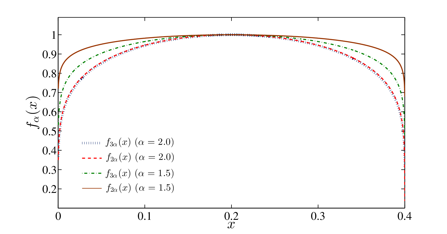
One can do the same calculations also for the configurations $\mathfrak{C_{2}}$ (in this case we considered $l=L/2$ and $S\sim\frac{\tilde{c}_{2}^{F}(\alpha)}{3}\log L$) and $\mathfrak{C_{3}}$ (where we take $S\sim\frac{\tilde{c}_{3}^{F}(\alpha)}{6}\log L$). In Fig. (9) we sketched $\tilde{c}^{F}(\alpha)$. It is clear that the results for different configurations $\mathfrak{C_{2}}$, $\mathfrak{C_{3}}$ and $\mathfrak{C_{4}}$ are similar. In other words

$$c^{F}(\alpha)=c^{F}_{2}(\alpha)=c^{F}_{3}(\alpha)=c^{F}_{4}(\alpha)$$

(44)

In the next section we will discus this similarity and we will show that these results are also the same as the massive systems. In case $\mathfrak{C_{3}}$ to have an idea about the function which controls the finite size effect we first realized that one can fit the data to the following function

$$S=\frac{c^{F}_{3}(\alpha)}{6}\log(Lf_{3\alpha}(\frac{l}{L})),$$

(45)

where $f_{\alpha}(x\to 0)\sim x$ and $f_{\alpha}(\frac{1}{2})\sim 1$. One can determine the function $f_{\alpha}$ by using the formula

$$f_{3\alpha}(\frac{l}{L})=e^{\frac{6}{c^{F}_{3}(\alpha)}(S_{\alpha}(l)-S_{\alpha}(\frac{L}{2}))}.$$

(46)

As one can see in Fig (10) the function is smoothly $\alpha$ dependent. At the same Fig (10) we also depicted the same function for the case $\mathfrak{C_{2}}$ where we define $f_{2\alpha}(\frac{l}{L})=e^{\frac{3}{c^{F}_{2}(\alpha)}(S_{\alpha}(l)-S_{\alpha}(\frac{L}{2}))}$. It seems that except at the $\alpha=2$ the form of the functions are different in two different configurations.

References

- [1] L. Amico, R. Fazio, A. Osterloh, and V. Vedral, Rev. Mod. Phys. 80, 517 (2008)
- [2] K. Modi, A. Brodutch, H. Cable, T. Paterek and V. Vedral, Rev. Mod. Phys. 84 (2012) 1655–1707
- [3] J. Eisert, M. Cramer and M. B. Plenio, Rev. Mod. Phys. 82, 277 (2010)
- [4] P. Calabrese and J. Cardy, J.Phys.A 42:504005,(2009)
- [5] H. Casini and M. Huerta, J.Phys.A42:504007 (2009)
- [6] I. Peschel and V. Eisler, J. Phys. A: Math. Theor. 42 504003 (2009)
- [7] L. Bombelli, R. K. Koul, J. Lee and R. D. Sorkin, Phys. Rev. D 34, 373 (1986).
- [8] M. Srednicki, Phys. Rev. Lett. 71, 666, (1993).
- [9] C. Callan, and F. Wilczek, Phys. Lett. B 333, 55 (1994).
- [10] I. Peschel, J. Phys. A: Math. Gen. 36 No 14, L205-L208 (2003)
- [11] O.A. Castro-Alvaredo and B. Doyon, J.Phys.A42:504006 (2009)
- [12] J. I. Latorre, R. Orús, E. Rico and J. Vidal, Phys. Rev. A, 71 (2005) 064101; T. Barthel, S. Dusuel and J. Vidal, Phys. Rev. Lett., 97 (2006) 220402; J. Vidal, S. Dusuel and T. Barthel, J. Stat. Mech., (2007) P01015; S. Dusuel and J. Vidal, Phys. Rev. B, 71 (2005) 224420; M. Filippone, S. Dusuel and J. Vidal, Phys. Rev. A 83, 022327 (2011)
- [13] R. Orus, S. Dusuel and J. Vidal, Phys. Rev. Lett. 101, 025701 (2008); M. Filippone, S. Dusuel and J. Vidal, Phys. Rev. A 83, 022327 (2011)
- [14] W. Dür, L. Hartmann, M. Hein, M. Lewenstein and H. J. Briegel, Phys. Rev. Lett. 94, 097203 (2005).
- [15] T. Koffel, M. Lewenstein and L. Tagliacozzo, Phys. Rev. Lett. 109, 267203 (2012).
- [16] J. Eisert and T. J. Osborne, Phys. Rev. Lett. 97, 150404 (2006) [quant-ph/0603114]; S. Bravyi, M. B. Hastings and F. Verstraete, Phys. Rev. Lett. 97, 050401 (2006) [quantph/ 0603121
- [17] M. B. Plenio, J. Eisert, J. Dreißig and M. Cramer, Phys. Rev. Lett. 94, 060503 (2005)
- [18] M. Cramer, J. Eisert, M.B. Plenio and J. Dreißig, Phys. Rev. A 73, 012309 (2006)
- [19] K. M. R. Audenaert, J. Eisert, M. B. Plenio, and R. F. Werner, 2002, Phys. Rev. A 66, 042327; C. H. Bennett, D. P. DiVincenzo, J. A. Smolin and W. K. Wootters , Phys. Rev. A 54, 3824 (1996).
- [20] A. Botero and B. Reznik, Phys. Rev. A 70, 052329 (2004)
- [21] M. Cramer and J. Eisert, New J. Phys. 8, 71 (2006)
- [22] A. Cadarso, M. Sanz, M. M. Wolf, J. I. Cirac and D. Perez-Garcia, Phys. Rev. B 87, 035114 (2013)
- [23] O.A. Castro-Alvaredo and B. Doyon, Phys. Rev. Lett., 108, 120401 (2012); P. Sadhukhan and S. M. Bhattacharjee, J. Phys. A: Math. Theor. 45 (2012) 425302; H. Katsura, Y. Hatsuda, J. Phys. A 40 (2007) 13931; D. Giuliano, A. Sindona, G. Falcone, F. Plastina and L. Amico, New J. Phys. 12 (2010) 025022, Philippe Corboz, Frederic Mila, [arXiv:1212.2983]; Shaon Sahoo, V. M. L. Durga Prasad Goli, S. Ramasesha and Diptiman Sen, J. Phys.: Condens. Matter 24, 115601 (2012); Rebecca Ronke, Tim Spiller and Irene DÁmico, J. Phys.: Conf. Ser. 286 (2011) 012020
- [24] M. G. Nezhadhaghighi and M. A. Rajabpour, EPL 100, 60011 (2012) [arXiv:1209.1883]
- [25] T. Blanchard, M. Picco, M. A. Rajabpour, EPL 101 (2013) 56003 [arXiv:1211.6758]
- [26] A. Zoia, A. Rosso and M. Kardar, Phys. Rev. E 76, 021116 (2007)
- [27] R. G. Unanyan and M. Fleischhauer, Phys. Rev. Lett. 95, 260604 (2005)
- [28] C. Holzhey, F. Larsen and F. Wilczek, Nucl. Phys. B 424, 443 (1994)
- [29] J. Eisert and M. Cramer, Phys. Rev. A 72, 042112 (2005) and R. Orús1, J. I. Latorre1, J. Eisert and M. Cramer, Phys. Rev. A 73, 060303 (2006)
- [30] Ingo Peschel and Jize Zhao, JSTAT P11002 (2005)
- [31] P. Calabrese and J. Cardy, J. Stat. Mech. P06002 (2004)
- [32] P. Calabrese, J. Cardy and I. Peschel, J.Stat.Mech.1009:P09003 (2010)
- [33] J. C. Xavier and F. C. Alcaraz, Phys. Rev. B 85, 024418 (2012)
- [34] S. G. Samko, A. A. Kilbas and O. I. Marichev, Fractional Integrals and Derivatives Theory and Applications, Gordon and Breach, New York (1993); M. Ilic, F. Liu, I. Turner, and V. Anh, Fractional Calculus and Applied Analysis 8.3, 324 (2005).
- [35] B. Swingle and T. Senthil, [arXiv:1112.1069].
- [36] H. Casini and M. Huerta, Nucl.Phys. B 764, 183-201(2007)
- [37] M.M. Wolf, F. Verstraete, M.B. Hastings and J.I. Cirac, Phys. Rev. Lett. 100, 070502 (2008)
- [38] Jean-Marie Stéphan, Shunsuke Furukawa, Grégoire Misguich and Vincent Pasquier, Phys. Rev. B 80, 184421 (2009)
- [39] Jean-Marie Stéphan, Grégoire Misguich and Vincent Pasquier, Phys. Rev. B 82, 125455 (2010) and Phys. Rev. B 84, 195128 (2011); Michael P. Zaletel, Jens H. Bardarson and Joel E. Moore, Phys.Rev.Lett. 107, 020402 (2011)
- [40] J. Wilms, M. Troyer and F. Verstraete, J. Stat. Mech. (2011) P10011; J. Wilms, J. Vidal, F. Verstraete and S. Dusuel, J. Stat. Mech. P01023 (2012)
- [41] Jaegon Um, Hyunggyu Park and Haye Hinrichsen, J. Stat. Mech. (2012) P10026
- [42] F. C. Alcaraz and M.A. Rajabpour, [arXiv:1305.1239 ]
- [43] H. Widom, Am. J. Math. 95, 333 (1973)