Orthogonal Range Searching for Text Indexing
Abstract
Text indexing, the problem in which one desires to preprocess a (usually large) text for future (shorter) queries, has been researched ever since the suffix tree was invented in the early 70’s. With textual data continuing to increase and with changes in the way it is accessed, new data structures and new algorithmic methods are continuously required. Therefore, text indexing is of utmost importance and is a very active research domain.
Orthogonal range searching, classically associated with the computational geometry community, is one of the tools that has increasingly become important for various text indexing applications. Initially, in the mid 90’s there were a couple of results recognizing this connection. In the last few years we have seen an increase in use of this method and are reaching a deeper understanding of the range searching uses for text indexing.
In this monograph we survey some of these results.
1 Introduction
The text indexing problem assumes a (usually very large) text that is to be preprocessed in a fashion that will allow efficient future queries of the following type. A query is a (significantly shorter) pattern. One wants to find all text locations that match the pattern in time proportional to the pattern length and number of occurrences.
Two classical data structures that are most widespread amongst all the data structures solving the text indexing problem are the suffix tree [104] and the suffix array [87] (see Section 2 for definitions, time and space usage).
While text indexing for exact matches is a well studied problem, many other text indexing related problems have become of interest as the field of text indexing expands. For example, one may desire to find matches within subranges of the text [86], or to find which documents of a collection contain a searched pattern [90], or one may want our text index compressed [93].
Also, the definition of a match may vary. We may be interested in a parameterized match [14, 85], a function match [5], a jumbled match [4, 24, 32, 89] etc. These examples are only a very few of the many different interesting ways that the field of text indexing has expanded.
New problems require more sophisticated ideas, new methods and new data structures. This indeed has happened in the realm of text indexing. New data structures have been created and known data structures from other domains have been incorporated for the use of text indexing data structures all mushrooming into an expanded, cohesive collection of text indexing methods. One of these incorporated methods is that of orthogonal range searching problems.
Orthogonal range searching refers to the preprocessing of a collection of points in -dimensional space to allow queries on ranges defined by rectangles whose sides are aligned with the coordinate axes (orthogonal).
In the problems we consider here we assume that all input point sets are in rank space, i.e., they have coordinates on the integer grid . The rank-space assumption can easily be made less restrictive, but we do not dwell on this here as the rank-space assumption works well for most of the results here.
The set of problems one typically considers in range searching are queries on the range such as emptiness, reporting (all points in the range), report any (one) point, range minimum/maximum, closest point. In general, some function on the set of points in the range.
We will consider different range searching variants in the upcoming sections and will discuss the time and space complexity of each at the appropriate place. For those interested in further reading of orthogonal range searching problems we suggest starting with [1, 27].
Another set of orthogonal range searching problems is on arrays (not point sets). We will lightly discuss this type of orthogonal range searching, specifically for Range Minimum Queries (RMQ).
In this monograph we take a look at some of the solutions to text indexing problems that have utilized range searching techniques. The reductions chosen are, purposely, quite straightforward with the intention of introducing the simplicity of the use of this method. Also, it took some time for the pattern matching community to adopt this technique into their repertoire. Now more sophisticated reductions are emerging and members of the community have also been contributing to better range searching solutions, reductions for hardness and more.
2 Problem Definitions and Preliminaries
Given a string , is the length of . Throughout this paper we denote . An integer is a location or a position in if . The substring of , for any two positions , is the substring of that begins at index and ends at index . The suffix of is the substring .
Suffix Tree The suffix tree [104, 101, 47, 88] of a string , denoted , is a compact trie of all the suffixes of (i.e., concatenated with a delimiter symbol , where is the alphabet set, and for all ). Each of its edges is labeled with a substring of (actually, a representation of it, e.g., the start location and its length). The “compact” property is achieved by contracting nodes having a single child. The children of every node are sorted in the lexicographical order of the substrings on the edges leading to them. Consequently, each leaf of the suffix tree represents a suffix of , and the leaves are sorted from left to right in the lexicographical order of the suffixes that they represent. requires space. The suffix tree can be prepared in , where is the text size, is the alphabet, and is the time required to sort the set [47]. For the suffix tree one can search an -length pattern in , where is the number of occurrences of the pattern. If the alphabet is large this potentially increases to , as one need to find the correct edge exiting at every node. If randomization is allowed then one can introduce hash functions at the nodes to obtain , even if the alphabet is large, without affecting the original construction time.
Suffix Array The suffix array [87, 71] of a string , denoted , is a permutation of the indices indicating the lexicographic ordering of the suffixes of . For example, consider . The suffix array of is , that is , where denotes less-than lexicographically. The construction time of a suffix array is [71]. The time to answer an query of length on the suffix array is [87]11 1 This requires LCP information. Details appear in Section 3.1.. The is required to find the range of suffixes (see Section 3.1 for details) which have as a prefix and then since appears as a prefix of suffix it must appear at location of the string . Hence, with a scan of the range we can report all occurrences in additional time.
Relations between the Suffix Tree and Suffix Array Let be a string. Let be its suffix array and its suffix tree. Consider ’s leaves. As these represent suffixes and they are in lexicographic ordering, is actually a tree over . In fact, one can even view as a search tree over .
Say we have a pattern whose path from the root of ends on the edge entering node in (the locus). Let denote the leftmost leaf in the subtree of and denote the rightmost leaf in the subtree of . Assume that is the location of that corresponds to , i.e. the suffix is associated with . Likewise assume corresponds to . Then the range contains all the suffixes that begin with and it is maximal in the sense that no other suffixes begin with . We call this range the -range of .
Consider the previous example with suffix array . For a query pattern we have that the -range for is , i.e. is a common prefix of .
Beforehand, we pointed out that finding the -range for a given takes in the suffix array. However, given the relationship between a node in the suffix tree and the SA-range in the suffix array, if we so desire, we can use the suffix tree as a search tree for the suffix array and find the SA-range in time. For simplification of results, throughout this paper we assume that indeed we find -ranges for strings of length in time.
Moreover, one can find for all nodes in a suffix tree representing for in time using suffix links. Hence, one can find all -ranges for for in time.
3 1D Range Minimum Queries
While the rest of this paper contains results for orthogonal range searching in rank space, one cannot disregard a couple of important range searching results that are widely used in text indexing structures. The range searching we refer to is the Range Minimum Query (RMQ) problem on an array (not a point set). RMQ is defined as follows.
Let be a set of linearly ordered elements whose elements can be compared (for ) in constant time.
| -Dimensional Range Minimum Query (d-RMQ) | |
|---|---|
| Input: | A d-dimensional array over of size |
| where is the size of dimension . | |
| Output: | A data structure over supporting the following queries. |
| Query: | Return the minimum element in a range |
| of . | |
1-dimensional RMQ plays an important role in text indexing data structures. Hence, we give a bit of detail on results about RMQ data structure construction.
The 1-dimensional RMQ problem has been well studied. Initially, Gabow, Bentley and Tarjan [53] introduced the problem. They reduced the problem to the Lowest Common Ancestor (LCA) problem [61] on Cartesian Trees [103]. The Cartesian Tree is a binary tree defined on top of an array of elements from a linear order. The root is the minimum element, say at location of the array. The left subtree is recursively defined as the Cartesian tree of the sub-array of locations to and the right subtree is defined likewise on the sub-array from to . It is quite easy to see the connection between the RMQ problem and the Cartesian tree, which is what was utilized in [53], where the LCA problem was solved optimally in time and space while supporting time queries. This, in turn, yielded the result of preprocessing time and space for the 1D RMQ problem with answers in time.
Sadakane [97] proposed a position-only solution, i.e. one that return the position of the minimum rather than the minimum itself, of bits space with query time. Fischer and Heun [52] improved the space to bits and preprocessed in time for subsequent time queries. They also showed that the space must be of size . Davoodi, Raman and Rao [41] showed how to achieve the same succinct representation in a different way with working space, as opposed to the working space in [52]. It turns out that there are two different models, the encoding model and the indexing model. The model difference was already noted in [43]. For more discussion on the modeling differences see [22]. In the encoding model we preprocess the array to create a data structure enc and queries have to be answered using enc only, without access to . In the indexing model, we create an index idx and are able to refer to when answering queries. The result of Fischer and Heun [52] is the encoding model result. For the indexing model Brodal et al. [22] and Fischer and Heun [52], in parallel, showed that an index of size bits is possible with query time . Brodal et al. [22] showed that this is an optimal tradeoff in the indexing model.
Range minimum queries on an array have been extended to 2D in [8, 13, 22, 21, 42, 56] and to higher dimension in [22, 30, 13, 40].
3.1 The LCP Lemma
The Longest Common Prefix (LCP) of two strings plays a very important role in text indexing and other string matching problems. So, define as follows.
Definition 1
Let and be two strings over an alphabet . The longest common prefix of and , denoted , is the largest string that is a prefix of both and . The length of is denoted .
The first sophisticated use of the LCP function for string matching was for string matching with errors in a paper by Landau and Vishkin [82]. An interesting and very central result to text indexing structures appears in the following lemma, which is not difficult to verify.
Lemma 1
[87] Let be a sequence of lexicographically ordered strings. Then .
This allows a data structure over the suffix array of size that returns the LCP value of any two substrings in time. This is done by building an RMQ data structure over the array containing the values of the LCP of lexicographically consecutive suffixes and using the lemma.
This result was implicitly22 2 They did not actually use the RMQ data structure. Rather, since they know the path a binary search will follow, they know which interval one needs to (RMQ)query when consulting a given suffix array position (there is only one path towards it in the virtual binary search tree). So they directly store that range LCP value. used in [87] to reduce the time for a search of an -length pattern in a suffix array indexing a text of length to . The idea is as follows. Both find the -range for based on a binary search of the pattern on the suffixes of the suffix array. The time follows for a naive binary search because it takes time to check if is a prefix of a suffix and the follows from the binary search.
Reducing to is done as follows. The binary search is still used. Initially is compared to the string in the center of the lexicographic ordering. This may take time. However, at every stage of the binary search we maintain for the suffix of with the maximal , over all the suffixes to which has already been compared. When comparing to the next suffix, say , in the binary search, first is evaluated (in constant time) if we immediately know the value of - give it a moment of thought - and we can compare the character at location +1 of and and continue the binary search from there. Otherwise, in which case we continue the comparison of and (but only) from the +1-th character. Hence, one can claim, in an amortized sense, that the pattern is scanned only once. So, the search time is .
The dynamic version of this method is much more involved but has interesting applications, see [9].
3.2 Document Retrieval
The Document Retrieval problem is very close to the text indexing problem. Here we are given a collection of documents and desire to preprocess them in order to answer document queries . A document query asks for the set of documents where appears.
The generalized suffix array (for generalized suffix tree, see [60]) is a suffix array for a collection of texts and can be viewed as the suffix array for . However, we may remove, before finalizing the suffix array, all suffixes that start with a delimiter as they contain no interesting information. In order to solve the document retrieval problem one can build a generalized suffix array for . The problem is that when one seeks a query one will find all the occurrences of in all documents, whereas we desire to know only in which documents appears and are not interested in all match locations.
A really neat trick to solve this problem was proposed by Muthukrishnan [90]. Imagine the generalized suffix array for of size and a document retrieval query of length . In , or even in time (as discussed in the end of Section 2) it is possible to find the -range for . Now we’d like to report all documents who have a suffix in this range. So, create a document array for the suffix array. The document array for will be of length and will contain at location the document id if is a suffix beginning in document . So, the former problem now becomes the problem of finding the unique id’s in the -range of the document array.
Muthukrishnan [90] proposed a transformation to the RMQ problem in the following sense. Take the document array and generate, yet another, array which we will call the predecessor document array. Let if , and for all . if there is no such . The predecessor document array has at location . The following observation now follows.
Lemma 2
Let be a collection of documents and let be their generalized suffix array. Let be a query and let be the -range of . There is a one-one mapping between the documents in range in the document array and the values in range in the predecessor document array.
Proof
Let be all locations in where document id appears in the document array. Then the -th location of the predecessor document array will be . However, locations will contain , all greater than or equal to , in the predecessor document array. ∎
Hence, it is natural to consider an extended problem defined now.
| Bounded RMQ | |
|---|---|
| Input: | An array . |
| Output: | A data structure over supporting the following |
| bounded RMQ queries. | |
| Query: | Given a range and a number find all values in the |
| range of value . | |
The bounded RMQ problem can be solved by recursively applying the known RMQ solution. Find an RMQ on , say it is at location . If it is less than then reiterate on and . The preprocessing time and space are the same as those of the RMQ problem. The query time is , where is the number of elements smaller than .
This yields an solution for the document retrieval problem, where is the number of documents in which the query appears.
4 Indexing with One Error
The problem of approximate text indexing, i.e. the text indexing problem where up to a given number of errors is allowed in a match is a much more difficult problem than text indexing. The problem is formally defined as follows.
| Input: | Text of length over alphabet and an integer . |
|---|---|
| Output: | A data structure for supporting -error queries. |
| Query: | A -error query is a pattern of length over alphabet |
| for which we desire to find all locations in where matches | |
| with errors. |
We note that there are several definitions of errors. The edit distance allows for mismatches, insertions and deletions [84], the Hamming distance allows for mismatches only. For text indexing with errors (for Hamming distance, Edit distance and more) Cole et al. [35] introduced a novel data structure which, for the Hamming distance version, uses space (it is preprocessed within an factor of the space complexity) and answers queries in . See also [25, 100] for different space/time tradeoffs for the Hamming distance version.
Throughout the rest of this section we focus and discuss the special case of one error. Moreover, we will do so for the mismatch error, but a similar treatment will handle insertions and deletions. The reduction to range queries presented in this section was obtained in parallel by Amir et al. [10] and by Ferragina, Muthukrishnan and de Berg [50]. The goal of [50] was to show geometric data structures that solve certain methods in object oriented programming. They also used their data structure to solve the dictionary matching with one error. In [10] Amir et al. solved dictionary matching with one error and also solved the text indexing with one error. For the sake of simplicity, we will present the result of text indexing with one error from [10], but the reduction is the same for dictionary matching (see definition in [10]).
The algorithm that we will shortly describe combines a bidirectional construction of suffix trees, which had been known before. Specifically, it is similar to the data structure of [20]. However, in [20] a reduction to 2D range searching was not used.
4.1 Bidirectional Use of Suffix Arrays
For simplicity’s sake we make the following assumption. Assume that there are no exact matches of the pattern in the text. We will relax this assumption later and show how to handle it in Section 4.3.
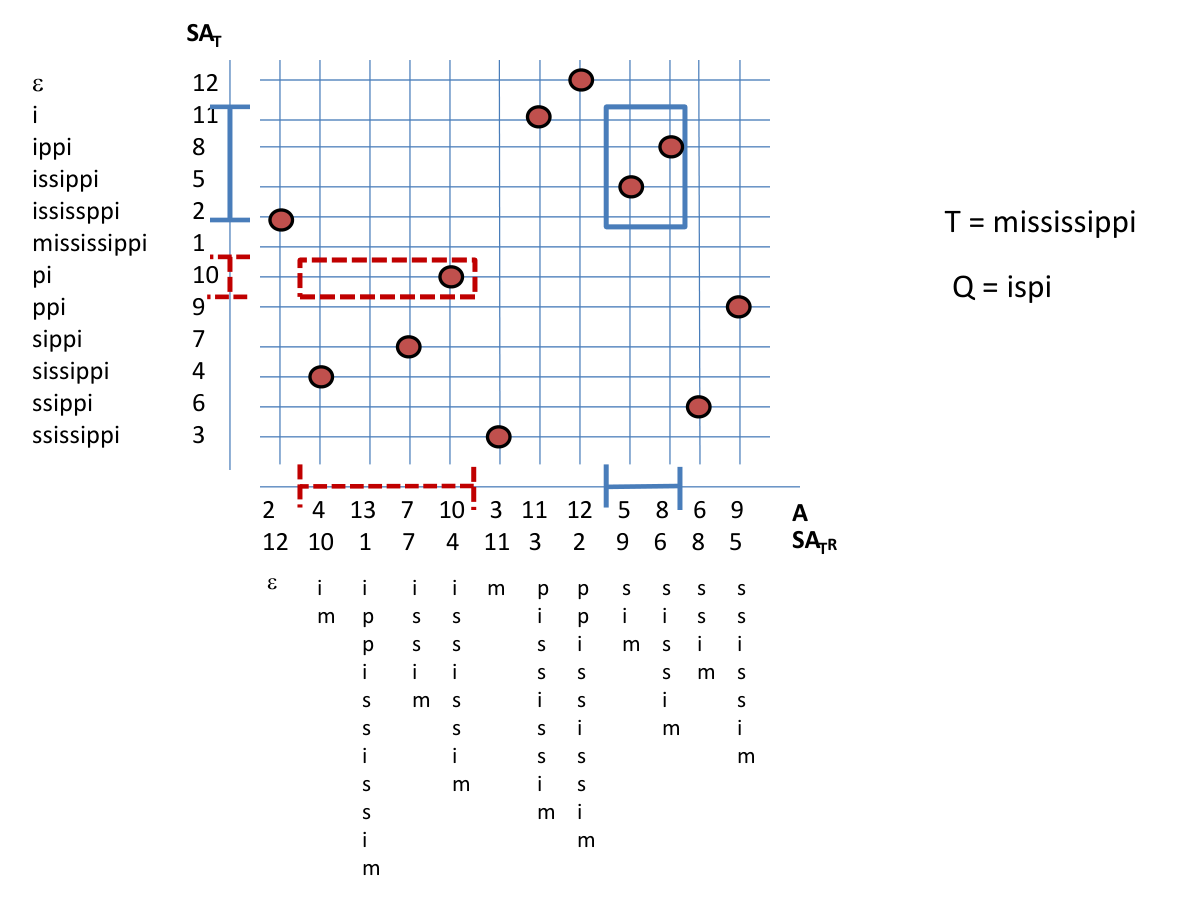
The main idea: Assume there is a pattern occurrence at text location with a single mismatch in location . This means that has an exact match at location and has an exact match at location .
The distance between location and location is dependent on the mismatch location, and that is somewhat problematic. We therefore choose to “wrap” the pattern around the mismatch. In other words, if we stand exactly at location of the text and look left, we see . If we look right we see . This leads to the following algorithm.
For the data structure supporting -mismatch queries construct a suffix array of text string and a suffix array of the string , where is the reversed text .
In order to reply to the -mismatch queries do as follows:
Query Reply:
-
For do
- 1.
Find the maximal -range of in , if it is non-empty.
- 2.
Find the maximal -range of in , if it is non-empty.
- 3.
If both and are non-empty, then return the intersection of and on their respective ranges.
Steps 1 and 2 of the query reply can be done for the ’s in overall linear time (see end of Section 2). Hence, we only need an efficient implementation of Step 3.
4.2 Set Intersection via Range Reporting
In Step 3, given -ranges [] and [] we want to report the points in the intersection of and w.r.t. to the corresponding coordinates of the two ranges. We show that this quite straightforwardly reduces to the 2D range reporting problem.
| Range Reporting in 2D (rank space) | |
|---|---|
| Input: | A point set . |
| Output: | A data structure representing that supports the following |
| range reporting queries. | |
| Query: | Given a range report all points of |
| contained in . | |
Since the arrays (the suffix array for and the suffix array for ) are permutations, every number between 1 and (we include suffix ) appears precisely once in each array. The coordinates of every number are , where and (the choice of is to align the appropriate reverse suffix with suffix — explanation: becomes when reversing the text. Then one needs to move over one to the mismatch location and one more to the next location). We define the point set to be and construct a range reporting structure for it (efficiency to be discussed in a moment). It is clear that the range elements intersection corresponds precisely with a query .
The current best range reporting data structures in 2D are as follows:
- 1.
Alstrup, Brodal and Rauhe [2]: a data structure requiring space, for any constant , that can answer queries in , where is the number of points reported.
- 2.
Chan, Larsen and Pǎtraşcu [27]: a data structure requiring space that can answer queries in .
- 3.
Chan, Larsen and Pǎtraşcu [27]: a data structure requiring space that can answer queries in . Other succinct results of interest appear in a footnote33 3 Note that prior succinct solutions show a novel adaptation of the method of Chazelle [28] to Wavelet Trees [58], see [70], [86] and [15]. It is especially worth reading the chapter of ”Application as Grids” in [91] for more results along this line..
Therefore, we have the following.
Theorem 4.1
Let and . When no exact match exists, indexing with one error can be solved with space such that queries can be answered in time, where:
-
s(n) = the space for a range reporting data structure and
-
occ = the number of occurrences of in with one error, and
-
qt(n,m,occ) = the query time for the same range reporting data structure.
Proof: Other than the range reporting data structure the space required is . Likewise, Steps 1 and 2 of the query response require total time for . Hence, the space and time are dominated by the range reporting data structure at hand, i.e. space and query time . ∎
4.3 Indexing with One Error when Exact Matches Exist
We assumed that the text contained no exact pattern occurrence in the text. In fact, the algorithm would also work for the case where there are exact pattern matches in the text, but its time complexity would suffer. Recall that the main idea of the algorithm was to pivot a pattern position and check, for every text location, whether the pattern to the left and to the right of the pivot were exact matches. However, if the pattern occurs as an exact match in the text then at that occurrence a match is announced for all pivots. So, this means that every exact occurrence is reported times. The worst case could end up being as bad as (for example if the text is and the pattern is then it would be ).
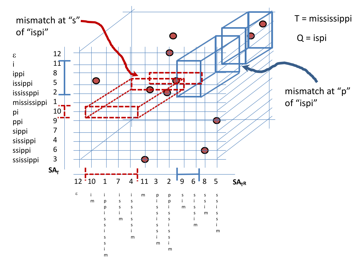
To handle the case of exact occurrences one can use the following idea. Add a third dimension to the range reporting structure representing the character in the text at the mismatch location. The desired intersection is of all suffix labels such that this character is different from the symbol at that respective pattern location. This leads to a specific variant of range searching.
| 3D 5-Sided Range Reporting (rank space) | |
|---|---|
| Input: | A point set |
| . | |
| Output: | A data structure representing that supports the |
| following range reporting queries. | |
| Query: | Given a range report all points |
| of contained in . | |
3D 5-Sided Range Reporting can be solved with space and query time [27].
Back to our problem. We need to update the preprocessing phase.
Preprocessing: Preprocess for 3-dimensional range queries on the matrix . If is unbounded, then use only the symbols in . The new geometric points are , where and will be the same as before and will be the text character that needs to mismatch. This will be added in the preprocessing stage.
The only necessary modification is for Step 3 of the query reply which becomes:
- 3.
If and both exist, then return all the points in for which the z-coordinate is not the respective pattern mismatch symbol.
The above step can be implemented by two 3D 5-sided range queries on the three dimensional range and where is the current pattern symbol being examined. We assume that the alphabet symbols are numbered .
See Figure 2 depicting the 3D queries.
Theorem 4.2
Let and . Indexing with one error can be solved with space and query time, where is the number of occurrences of the pattern in the text with at most one error.
4.4 Related Material
For a succinct index for dictionary matching the best result appears in [62].
A wildcard character is one that matches all other symbols. When used we denote them with .
Iliopoulos and Rahman [67] consider the problem of indexing a text to answer queries of the form , where and are known during the preprocessing. The is known as gap-indexing. Bille and Gørtz [18] consider the same problem. However, they required only to be known in advance. The solution in [18] uses a reduction to range reporting. The reduction they apply is similar to the one presented in this chapter. In fact, it is easier because the gap’s location within the query pattern is known. So, one does not need to check every position of the pattern as one does in the case of mismatch. Hence, the 2D range reporting data structure is sufficient. One does need to adapt the search for a difference of instead of . This requires setting .
5 Compressed Full-Text Indexes
Given that texts may be very large it makes sense to compress them - and there are many methods to do so. On the other hand, these are not constructed to allow text indexing. Doing both at once has been the center of a lot of research activity over the last decade. However, reaching this stage has happened in phases. Initially, pattern matching on compressed texts was considered starting by Amir et al. [6]. By pattern matching on compressed texts we mean that a compressed text, with some predefined compressor, and a pattern are given and the goal is to find the occurrences of the pattern efficiently without decompressing the text. The second phase was text indexing while maintaining a copy of the original text and augmenting it with some sublinear data structure (usually based on a compressor) that would allow text indexing, e.g. [72]. We will call this phase, the intermediate phase. Finally, compressed full-text indexing was achieved, that is text indexing without the original text and with a data structure with size depending on the compressibility of the string. See Section 3 for the discussion on the encoding model vs. the indexing model. Compressed full-text indexes of note are that of Ferragina and Manzini [49], the FM-Index, that of Grossi and Vitter [59], the Compressed Suffix Array and that of Grossi, Gupta and Vitter [58], the Wavelet Tree. For an extensive survey on compressed full-text indexes see [93].
In this section we will present two results, that of Kärkkäinen and Ukkonen [72] and that of Claude and Navarro [33]. The latter uses a central idea of the former. However, the former is from the intermediate phase. So, it maintains a text to reference. This certainly makes the indexing easier. The latter is a compressed full-text index. The former uses the more general LZ77 and the latter uses SLPs (Straight Line Programs). Both LZ77 and SLP compressions are defined in this section.
5.1 LZ77 Compressed Indexing
The Lempel-Ziv compression schemes are among the best known and most widely used. In this section (and in Section 7) we will be interested in the variant known as LZ77 [107]. For sake of completeness we describe the LZ77 scheme here.
An Overview of the Lempel-Ziv Algorithm
Given an input string of length , the algorithm encodes the string in a greedy manner from left to right. At each step of the algorithm, suppose that we have already encoded with phrases (phrase - to be defined shortly). We search for the location , such that , for which the longest common prefix of and the suffix is maximal. Once we have found the desired location, suppose the aforementioned longest common prefix is the substring , a phrase, , will be added to the output which will include the encoding of the distance to the substring (i.e., the value ), the length of the substring (i.e., the value ), and the next character . The algorithm continues by encoding . The sequence of phrases is called the string’s (LZ77) parse and is defined:
We denote with the start location of in the string . Finally, we denote the output of the LZ77 algorithm on the input as .
Kärkkäinen and Ukkonen Method.
Farach and Thorup [46], in their paper on search in LZ77 compressed texts, noted a neat, useful observation. Say of length is the text to be compressed and is its LZ parse containing phrases.
Lemma 3
[46] Let be a query pattern and let be the smallest integer such that . Then for some .
In other words, the first appearance of in cannot be contained in a single phrase. Kärkkäinen and Ukkonen [72] utilized this lemma to show how to augment the text with a sublinear text indexing data structure based on LZ77.
The idea is as follows. Say we search for a pattern in the text which has been compressed by LZ77. The occurrences of in are defined differently for those that intersect with more than one phrase (which must exist if there are any matches according to Lemma 3) and those that are completely contained in a single phrase. The former are called primary occurrences and the latter are called secondary occurrences. The algorithm proposed in [72] first finds primary occurrences and then uses the primary occurrences to find secondary occurrences. Both steps use orthogonal range searching schemes.
In order to find the primary occurrences they used a bi-directional scheme based on Lemma 3. Take every phrase and creates its reverse . Now, consider a primary occurrence and the first phrase it starts in, say . Then there must be a such that is a suffix of and is a prefix of the suffix of , . So, to find the primary occurrences it is sufficient to find such that:
- 1.
is a prefix of .
- 2.
is a prefix of the suffix of .
Let be the lexicographic sort of , i.e. . This leads to a range reporting scheme, similar to that of the previous section, of size , where the point set .
Therefore, for every we need to (1) find the range of for which every within has as a prefix and (2) find the range of suffixes that have as a prefix. Once we do so we revert to range reporting, as in the previous section. However, finding the ranges is not as simple as in the previous section. Recall that we want to maintain the auxiliary data in sublinear space. So, saving a suffix array for the text is not a possibility. Also, the reversed phrases need to be indexed for finding the range of relevant phrases.
To this end a sparse suffix tree was used in [73]. A sparse suffix tree is a compressed trie over a subset of the suffixes and is also known as a Patricia Trie over this suffix set. As it is a compressed trie it is of size subset size, in our case . Lately, in [17] it was shown how to construct a sparse suffix array in optimal space and near-optimal time.
The sparse suffix tree can be constructed for the suffixes and, since we have the original text on hand, we can maintain the compressed suffix tree in words. Navigation on this tree is the same as in a standard suffix tree. For the reversed phrases we can associate each with a prefix of the text. Reversing them gives a collection of suffixes of the reversed text. Now construct a sparse suffix tree for these reversed suffixes and this will allow finding the range in (with the help of the existing text) as in the previous section. Hence,
Theorem 5.1
Let be a text and its LZ77 parse. One can construct a text indexing scheme which maintains along with a data structure of size such that for a query we can find all its primary occurrences in , where is the number of primary occurrences.
Proof
For the query , as described above, each pattern position is evaluated for primary occurrences. That is for each of the pattern positions, we first traverse the auxiliary sparse suffix trees in time and once the ranges (for that pattern position is found) we perform a range query. The traversal will cost time.
Using the 2D succinct range reporting of Chan et al. [27] (see previous section) we have linear space, i.e. , and query time where is the number of points found, which is the same as the number of primary occurrences found.
Hence, over the pattern positions the range querying will cost time, where is the number of primary occurrences when we split the pattern at position . However, . Recalling that the traversal cost time yields the desired. ∎
We note that the secondary occurrences still need to be found. This is another interesting part of the paper and we refer the interested reader to [72].
5.2 SLP Text Indexing
Claude and Navarro [33] proposed a full-text indexing scheme based on straight line programs (SLPs). An SLP is a grammar based compression for a text . The grammar produces exactly one word and the rules are in Chomsky Normal Form, i.e. each rule is , where are variables of the grammar or , where is a variable and is a terminal (a character of ).
The text indexing scheme that they propose follows the previous idea [72] of finding primary and secondary occurrences. However, for SLPs things are slightly different. Consider the derivation tree for the text , that is deriving the full word by generating from the start symbol as the root (if then and will be children of the root in the derivation tree - from here the derivation tree is applied recursively until the full is spelled out in the left-to-right order of the leaves). Every occurrence of a pattern in the text has a unique lowest variable which produces this occurrence, but its children do not. That is if the children of are and , i.e. there is a rule , then produces (where ) and produces (where ) for some . We say that splits pattern at location . An occurrence of is called a primary occurrence if for some and splits this occurrence of . All other occurrences are secondary occurrences.
The format of the algorithm is to, once again, find the primary occurrences and then to deduce the occurrences of in the text therefrom. With the goal of finding the primary occurrences in mind, once again, our grid will be of size , where is the size of the variable set of the grammar. Each side of the grid will have one coordinate for each variable. The range searching point set is defined per rule, . The location on the grid corresponding to (for ) on one side and (for ) on the other will have a point, , on the grid. The ordering of the variables on either side of the grid follows from the desire to satisfy the following conditions.
- 1.
is a prefix of .
- 2.
is a prefix of .
- 3.
There is a rule .
It is easy to see that the desired ordering, as in the LZ77 scheme, has the phrases in the -coordinate in reverse lexicographic ordering and has the phrases in the -coordinate in lexicographic ordering. The challenge here is to actually find the range of variables where is a prefix of . This is because it is a full-text index and the text is not accessible any more. Nevertheless, this is doable in the SLP compression scheme using a suffix array type of search and comparing with the variable at hand. This comparison is not trivial. However, the full scheme is out of scope of this survey and we refer the reader to the full paper [33]. The result achieved is as follows:
Theorem 5.2
Let be a text of size represented by an SLP with variables and height . There is a representation using bits such that of length can be found in query time.
6 Weighted Ancestors
6.1 2-Sided Sorted Range Reporting in 2D
In this section we consider the 2-sided sorted range reporting problem44 4 Results in Section 6.1 stem from wonderful research chats with Timothy Chan. which is defined now.
| 2-Sided Sorted Range Reporting in 2D | |
|---|---|
| Input: | A point set . |
| Output: | A data structure representing that supports the following |
| 2-sided sorted range reporting queries. | |
| Query: | Given a range report all points of |
| contained in sorted by their -coordinate | |
| (from highest to lowest). | |
Note that we deviate from the assumption that the points are in rank-space. This is important for the the application of this section. We now show a method to solve the 2-sided sorted range reporting. The idea is as follows.
Consider the dynamic predecessor problem in which we need to support the following operations (a) insertions/deletions of integers () and (b) predecessor queries. This is a classical problem and is solved with a van-Emde Boas tree [102] or with -fast tries [105] in space ( is the current number of integers) and time for the operations, where is the domain of the elements.
Dietz and Raman [44] asked whether this could be made partially persistent55 5 Actually Dietz and Raman [44] asked about persistency in general, which may refer to full persistence or partial persistence. We stick to partial persistence as it is sufficient for our needs. within the same query times. In other words can one create a data structure where insertions and deletions are supported on the current version but predecessor queries can be made on any of the versions (current or previous) of the data structure. Recently, Chan [26] accomplished this by constructing a partially persistent predecessor data structure with space and operations time . Chan’s result [26] is in fact more general, showing that the first predecessor can be found (in any previous version) in time but the predecessor of the predecessor (etc.) can be found in time. This yields a time of to find the previous elements in sorted order in a chosen version of the data structure.
We utilize this for the 2-sided sorted range reporting by creating a data structure for as follows66 6 We point out that for our purposes, finding one successor, the results of Dietz and Raman [44] are sufficient because (a) we seek only one successor and (2) the insertions are done first and then the queries are asked.. Consider the sort of the -coordinates of , i.e. some permutation for which . Now we insert the -coordinates into the data structure according to . That is we insert and then until . Now, a 2-sided sorted range reporting query is answered as follows; first use a predecessor query to find within - that is find such that . Then we go to the -th copy of the partially persistent data structure which contains the points . Hence, the points are exactly the points that satisfy that their -coordinate . Now to find the relevant points () in sorted by their -coordinate we need to apply the predecessor query. This yields an when using the data structure from [26]. Hence,
Theorem 6.1
The 2-sided sorted range reporting problem on an -point set over a grid can be solved with space and time.
6.2 Weighted Ancestors to 2-Sided Range Successor in 2D
Consider the weighted ancestors problem on an edge-weighted tree introduced by Farach and Muthukrishnan [45] for the sake of obtaining a perfect-hash for substrings. An edge-weighted tree is a tree where each edge has a weight . Each node is associated with a weight , where is the path from root-to-. The weighted ancestors problem is defined as follows.
Input: An edge-weighed tree with weight function .
Ouput: A data structure supporting weighted ancestor queries.
Query: Given a node and a threshold find the ancestor of such that , but , where is the parent of .
The weighted ancestor problem is a natural extension of the predecessor problem to trees. The application considered by [45] was on suffix trees. A suffix tree can be viewed as an edge-weighted tree with the edge weights denoting the length of the text with which the edge is marked. Now, say you are given indices and and want to find the locus of in the suffix tree. This can be done by going to the leaf representing and asking a weighted ancestor query with threshold . The answer to the query is the locus of .
In [45] a solution was given with preprocessing time, space, and query time. Their solution is based on a heavy path decomposition in order to linearize the input tree. Each path of the heavy path decomposition is assigned a predecessor structure. The preprocessing time of can be improved to and this has been pointed out in [11, 79]. It should be mentioned that the authors of [45] were considering a PRAM model and hence the time is really parallel time and work. Lately, it was shown that if the depth of the answer is in the tree then the query can be answered in time [78].
We now present a solution for this problem using 2-sided sorted range reporting.
Consider the edge-weighted input tree . We assume that every internal node in the tree has at least two children. Otherwise, create a dummy child with an arbitrary edge weight, say 1. Now consider the leaves ordered in inorder. For every two adjacent leaves denote their lowest common ancestor with and . With one scan of the tree all these values are computable. Now generate an array of the values. Say we are given a weighted ancestor query, node and threshold . We may assume that is a leaf. Otherwise, we simply choose a descendant leaf to represent (the answer will be the same). Consider the node which is the answer to the query and consider its parent . Since has at least two children has at least one sibling. Say, has a sibling to its left (in inorder). Let then in the array the first location that satisfies is the node for which the . To obtain this we revert to 2-sided sorted range reporting. We set the points on the grid to be . The query is bounded by in the -coordinates and in the -coordinates. What we are looking for is the first answer, the element with the largest -coordinate.
Note that once this is done it is still necessary to find (we only obtained ). This can be done with a predecessor structure for each node. That is, for each node save the index of the leftmost leaf for each of ’s children. A predecessor query with will return the correct edge with child , the weighted ancestor of . Hence,
Theorem 6.2
Let be an node edge-weighted tree with weights from . Then using 2-sided sorted range reporting one can answer weighted ancestor queries in time. The space required is .
Note that for a suffix tree, the motivation in [45], the weights are from . So, the query time for a suffix tree is .
Recall (from Section 3) the definition of an -range and its relation to the suffix tree. Hence, the method just described precisely finds the boundaries of the -range for a given suffix (in the suffix array) and its prefix of length (threshold) .
7 Compressed Substring Retrieval
In this section we are concerned with the substring compression problem. The substring compression problem was introduced in [36]. Some of the definitions and layout here are from [36]. The solution, specifically the reduction to range successor queries, is from [75].
In substring compression one is given a text to preprocess so that, upon request, a compressed substring is returned. The goal is to do so quickly, preferably in time, where is the size of the compressed substring. Generalized substring compression is the same with the following twist. The queries contain an additional context substring (or a collection of context substrings) and the answers are the substring in compressed format, where the context substring is used to make the compression more efficient.
The compressor of interest is, once again, LZ77. We use the terminology from Section 5. Some extra terminology is as follows. The string may be encoded within the context of the string . We denote this by . The encoded result will be equivalent to the result when LZ77 is performed on the concatenated string , where $ is a symbol that does not appear in either or . However, only the portion of which represents the compression of is output by the algorithm.
Formally, given a string of length , we wish to preprocess in such a way that allows us to efficiently answer the following queries:
- Substring Compression Query ():
-
given any two indices and , such that , we wish to output .
- Generalized Substring Compression Query ():
-
given any four indices , , , and , such that and , we wish to output .
The goal is to do answer queries quickly. Query times for both of the above query types will strongly depend on the number of phrases actually encoded. We denote these as and for SCQ and GSCQ, respectively.
7.1 SCQ to Range Successor in 2D
Recall the definition of LZ77 from Section 5. Imagine that we have already computed the phrases for and desire to compute the next phrase which is a prefix of . In other words, we want to find the location for which the longest common prefix of and the suffix is maximal. Consider the suffix , which is an extension of . Clearly, it is sufficient to find the suffix for which is maximized (without necessarily computing the value at this stage). Therefore we have two steps: (1) finding the location , and (2) computing . Step (2) is easy since we assume that we have a full LCP data structure as described in Section 3. So, our goal is to solve Step (1). To do so we generalize our problem to the following.
- Interval Longest Common Prefix ():
-
given , we look for location of for which the suffix has the longest common prefix with .
Clearly, for us it is sufficient to compute .
To compute the Interval Longest Common Prefix () we use a reduction to the problem of 3-sided range successor query. That is given a 2D rank-space input on an grid, a 3-sided query seeks the point in with the largest -coordinate. The 3-sided range successor query problem was considered under a different guise in [37] where it was called the range next value problem. There it was considered as an array problem for which one desires to preprocess the array to allow queries that seek the largest value on a range less than a value . This can be translated to a grid and vice versa.
7.2 4-Sided and 3-Sided Sorted Range Reporting
The 3-sided range successor query generalizes quite nicely to the 3-sided sorted range reporting in 2D which we define now.
| 3-Sided Sorted Range Reporting in 2D (rank space) | |
|---|---|
| Input: | A point set . |
| Output: | A data structure representing that supports the following |
| 3-sided sorted range reporting queries. | |
| Query: | Given a range report all points of |
| contained in sorted by their -coordinate | |
| (from highest to lowest). | |
A solution for the 3-sided range successor query problem was proposed in Lenhof and Smid [83]77 7 Note, they called it the Range Searching for Minimum problem., and modified in [76] (improved query times) to work in rank space, i.e. on an grid for values with queries supported in worst-case time, using space. However, there are now better results which solve, not only the 3-sided range successor problem, but the more general 3-sided sorted range reporting. The 3-sided sorted range reporting generalizes the 3-sided range successor query because the solutions presented can report the first location and stop.
For the same reason the 3-sided solutions work just as well for the 4-sided sorted range reporting, as they can report all points until the -coordinates surpasses the range boundary and then stop.
The current best range 3-sided sorted range reporting data structures in 2D are as follows:
- 1.
Navarro and Nekrich [95]:
(a): a data structure with space where queries can be answered in where is the number of points reported and
(b): a data structure with space where queries can be answered in and
(c): a data structure with space for any constant , where queries can be answered in , - 2.
Crochemore et al. [37]: a data structure that requires space for any constant and can answer queries in time.
7.3 The Interval Longest Common Prefix to 3-Sided Sorted Range Reporting
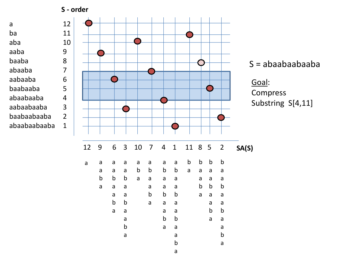
The reduction works as follows. Let be the suffix array of our input string of length . We associate each suffix with its string index and with its lexicographic index . From these two we generate a pair , where and . We then preprocess the set for 3-sided sorted range reporting queries. An example of the geometric representation of the scenario can be seen in Figure 3.
Computation of the ILCP Consider the suffix and the set of suffixes . Since , is in fact the suffix lexicographically closest to , out of all the suffixes of the set .
We will first assume that we are searching for a suffix , such that the suffix is lexicographically smaller than . The process for the case where the suffix chosen is lexicographically greater than is symmetric. Therefore, once both are found all we will need to do is to choose the best of both, i.e., the option yielding the greater value.
Since we have assumed w.l.o.g. that is lexicographically smaller than , we have actually assumed that , or equivalently, that appears to the left of in the suffix array. Incorporating the lexicographical ranks of and into the expression, is actually the value which maximizes the expression . Notice that .
Now consider the set . Assuming that indeed , we are interested in finding the maximal value , such that , and . It immediately follows that the point is the point in the range having the maximal -coordinate, and therefore can be obtained efficiently by obtaining the largest -coordinate in the output of the 3-sided sorted range query. Once we have found the point , we have , as .
Equivalently, there exists such that is the suffix lexicographically larger than and closest to it. In other words, we assume , or equivalently, that appears to the right of in the suffix array. can be found using a symmetric procedure. An example of the queries performed can be seen in Figure 4.

Determining whether or is implemented by calculating both and , and choosing the larger of the two. This gives us phrase . To finish simply reiterate. Hence,
Theorem 7.1
Let be a text of length . We can preprocess in space so that we can answer substring compression queries in time, where and are the space and query times mentioned above ().
The GSCQ problem
The generalized substring compression solution is more involved and uses binary searches on suffix trees applying range queries (3-sided range successor queries and emptiness queries) during the binary search. The interested reader should see [75].
Other applications
The reduction from this section to range searching structures, i.e. the set of , defined by a suffix with and had been considered beforehand.
This reduction was first used, to the best of our knowledge, by Ferragina [48] as part of the scheme for searching in a dynamic text indexing scheme. The reduction and point set were used also in position restricted substring search [86]. However, in both range reporting was used.
To the best of our knowledge, the first use of 3-sided range successor queries for text indexing was for range non-overlapping indexing and successive list indexing [76] and in parallel for position restricted substring search in [38].
See Section 9 for more range-restricted string search problems.
8 Top- Document Retrieval
The Top Document Retrieval problem is an extension of the Document Retrieval problem described in Section 3.2. The extension is to find the top documents in which a given pattern appears, under some relevance measure. Examples of such relevance measures are (a) tf(Q,d), the number of times occurs in document , (b) mind(Q,d), the minimum distance between two occurrences of and , (c) docrank(d), an arbitrary static rank assigned to document . In general, the type of relevance measures which which we shall discuss here are those that are defined by a function that assigns a numeric weight to every substring in document , such that depends only on the set of starting positions of occurrences of in . We call such a relevance measure a positions based relevance measure.
The following theorem is the culmination of the work of Hon, Shah and Vitter [65] and of Navarro and Nekrich [94].
Theorem 8.1
Let be a collection of strings (documents) of total length , and let be a positions based relevance measure for the documents . Then there exists an -word space data structure that, given a string and an integer reports documents containing of highest relevance, i.e. with highest values, in decreasing order of , in time.
Hon, Shah and Vitter [65] reduced this to a problem on arrays and achieved query time of . We will outline their idea within this section. Navarro and Nekrich [94] then showed how to adapt their solution to a 3-sided 2 dimensional range searching problem on weighted points. The solution of the range searching problem given in [94] builds upon earlier work on top color queries for document retrieval [74], another interesting result. We will describe the adaptation and range searching result shortly.
8.1 Flattening the Top- Document Retrieval Suffix Tree
Consider a generalized suffix tree for the document collection . The leaves have a one-one correspondence with the locations within the documents. If leaf is associated with location of document , we say that it is a -leaf. Let be the set of -leaves. Then a node is a -node if (a) it is a -leaf or if (b) it is an internal node of such that it is the lowest common ancestor of adjacent -leaves and . Let be a -node. If is is the lowest common ancestor of that is a -node we say that is ’s -parent (and that is ’s -child). If there is no lowest common ancestor of which is a -node then the -parent will be a dummy node which is the parent of the root. One can easily verify that the set of -nodes form a tree, called a -tree, and that an internal -node has at least two -children. It is also straightforward to verify that the lowest common ancestor of any two -nodes is a -node. Hence,
Lemma 4
Let be a node in the generalized suffix tree for the document collection . For every document for which the subtree of contains a -leaf there is exactly one -node in the subtree of that has a -parent to an ancestor of .
Proof
1. Every -parent of a -node in the subtree of is either in the subtree or is an ancestor of . 2. Assume, by contradiction, that there are two -nodes and in the subtree of each with a -parent that is an ancestor of . However, their lowest common ancestor, which must be a -node, is no higher than itself (since is a common ancestor). Hence, their -parents must be in ’s subtree a contradiction.
Hence, since every -node has a -parent, there must be exactly one -node with a -parent to an ancestor of . ∎
Corollary 1
Let be an arbitrary node in and let be a descendant of such that is a -node and its -parent is an ancestor of . Then all -nodes which are descendants of are also descendants of .
A node in may be a -node for different ’s, say for . Nevertheless, since every internal -node has at least two -children, the -tree is linear in the number of -leaves and, hence, the collection of all -trees is linear in the size of the which is .
In light of this in [65] an array was constructed by a pre-order traversal of the tree such that for each node which is a -node for indexes to are allocated in the array and contain the -parent of , , the -parent of . The integer interval denotes the interval bounded by the minimal and maximal indexes in assigned to or its descendants. Values and are stored in .
8.2 Solving with Weighted Range Searching
Let be the index in associated with -node for and with its -parent . Let be the string such that the locus of is . We generate a point , where denotes the depth of a node in the . The weight of the point is . Note that all points have different -coordinates and are on an integer grid.
It is still necessary to store a mapping from the -coordinates of points to the document numbers. A global array of size is sufficient for this task.
Queries. To answer a top- query first find the locus of (in time). Now, by Lemma 4 for each document containing there is a unique -node which is a descendant of with a -parent who is an ancestor of . By Corollary 1 , where is the string with locus , and is the weight of the point corresponding to the pointer from to its -parent. So, there is a unique point with and for every document that contains . Therefore, it is sufficient to report the heaviest weight nodes in . To do so Navarro and Nekrich [94] proposed the three sided top- range searching problem.
| Three sided top- range searching | |
|---|---|
| Input: | A set of weighted points on an grid . |
| Output: | A data structure over supporting the following queries. |
| Query: | Given and return the |
| heaviest weighted points in the range . | |
8.3 External Memory Top-k Document Retrieval
Lately, a new result for top- document retrieval for the external memory model has appeared in [98]. The result is I/O optimal and uses space.
9 Range Restricted String Problems
Research inspired by the problem of applying string problems limited to ranges has been of interest in the pattern matching community from around 2005. Some of the results are general. Others focus on specific applications. One such application is the substring compression problem that was discussed in Section 7. These problems are natural candidates for range searching solutions and indeed many of them have been solved with these exact tools.
The first three results on range restricted variants of text indexing appeared almost in parallel. The results were for property matching (the conference version of [7]), substring compression [36] and position-restricted substring searching [86].
Property matching
is the problem of generating a text index for a text and a collection of ranges over the text. The subsequent pattern queries asks for the locations where the text appears and are fully contained in some interval. The initial definition was motivated by weighted matching. In weighted matching a text is given with probabilities on each of the text symbols and each pattern occurrence in the text has weight which is the multiplication of the probabilities on the text symbols associated with that occurrence. Weighted matching was reduced to property matching. In [7] a solution was given using space, where is the text size, such that queries are answered in time, where is the pattern query and is the number of appearances within the interval set . The preprocessing time was near optimal and in a combination of a couple of papers was solved in optimal time [66, 69]. See also [39]. In [77] property matching was solved in the dynamic case, where intervals can be inserted and removed. Formally, denotes the collection of intervals and the operations are:
- •
Insert(, ) - Insert a new interval (, ) into .
- •
Delete(, ) - Delete the interval (, ) from .
In [77] it was shown how to maintain a data structure under interval deletions. Queries are answered in time and deletions take time. If both insertions and deletions are allowed then the insertion/deletion time is , where is the text length.
In [63] a succinct version was given that uses a compressed suffix array (CSA). The solution has a multiplicative logarithmic penalty for the query and update time.
Position-restricted substring searching
is the problem where the goal is to preprocess an index to allow range-restricted queries. That is the query consists of a pattern query and a range described by text indices and . This is different from property matching because the interval is not given a-priori. On the other hand, it is one interval only. The queries considered in [86] are position-restricted reporting and position-restricted counting. Another two related queries also considered are substring rank and substring select, which are natural extensions of rank and select [23, 57, 68]. These are defined as follows.
- 1.
PRI-Report: Preprocess text to answer queries Report, which reports all occurrences of in .
- 2.
PRI-Count: Preprocess text to answer queries Count, which returns the number of occurrences of in .
- 3.
Substring Rank: Preprocess text to answer queries SSR, which returns the number of occurrences of in .
- 4.
Substring Select: Preprocess text to answer queries SSS, which returns the occurrence of in .
We note that substring rank and position-restricted counting reduce to each other. Also, position-restricted reporting can be obtained from applying one substring-rank and substring-selects, where is the number of pattern occurrences in . We leave it to the reader to verify the details.
Reporting: For the reporting problem Mäkinen and Navarro [86] reduced the problem to range reporting. The way to do so is to first find the -range of . Then this range and the position-restricted range to define a rectangle for which range reporting is used. One can use any of the data structures mentioned in Section 4. For example with space, for any constant , one can answer queries in (we assume the alphabet is from otherwise if it is from then there is an extra additive factor of ). Crochemore et al. [38] noticed that a different type of reduction, namely range next value, could be more useful. The authors of [86] were more concerned with space issues. So, they also proposed a data structure which uses n + space and reports in . The reporting time was improved by Bose et al. [19] to with the same space constraints. Yu et al. [106] suggested a different algorithm with the same space and reporting time, but were able to report the occurrences in their original order.
Bille and Gørtz [18] went on to show that with space the query time can be improved to , which is optimal. They also solved position-restricted reporting merged with property matching. The space and query time remain the same.
An interesting result for the reporting variant appeared in [64]. Specifically, it was shown that a succinct space time index for position-restricted substring searching is at least as hard as designing a linear space data structure for 3D range reporting in time.
Counting: In [86] the same data structure that uses n + space and reports in was used for counting88 8 There is another result there that assumes faster query times that is flawed. See the introduction in [80] for an explanation.. Once again, Bose et al. [19] can improve the counting time to . Kopelowitz et al. [80] presented a counting data structure that uses space and answers counting queries in time . Recently, in the upcoming journal version of [18] a similar result appears. The space is the same. However, the counting time is , which can be slightly worse. Lately, Gagie and Gawrychowski [54] showed that if the alphabet is of size then space can be achieved. Moreover, if the alphabet size then they can reduce the query time to an optimal .
Substring Select: In [86] a solution for indexing for substring select is given. The space is , where is an upper bound on the size of the queried patterns. The query time is . This was improved in [80] to allow for any length query with space and optimal query time. The proposed solution in [80] uses persistent data structure which is a basic ingredient in most of the range searching solutions.
Substring compression
has been expanded on in Section 7. It was introduced in [36] and improved upon in [75]. The results are detailed in Section 7. One of the problems that is of interest in substring compression is the (interval longest common prefix) query. This inspired Amir et al. [3] to consider extensions to LCP range queries of different types.
Range non-overlapping indexing and successive list indexing [76]
. In range non-overlapping indexing one wants to prepare an index so that when give a pattern query one can return a maximal set of occurrences so that the occurrences do not overlap. In successive list indexing one prepares an index to answer queries where a pattern is given along with a position and one desires to find the first occurrence of the pattern after . A reduction to range successor was used to solve this problem. Along with the results of range sorted reporting [95] one can solve the former with space space and query time. For the latter the query time is .
Range Successor in 2D
solves several of the problems mentioned in this section. This has been discussed in Section 7 and is referred to in [37, 95, 106]. It is interesting that its generalization sorted range reporting [95] is a variant of range reporting that was considered in the community because of the unique range search problems that arise.
10 Lower Bounds on Text Indexing via Range Reporting
A novel use of range searching is its use to show lower bounds on text indexing via reductions from range reporting [31].
Theorem 10.1
Let be a set of points in . We can construct a text of length bits along with bits of auxiliary data such that we can answer range reporting queries on with pattern match queries on , each query is a pattern of length .
We denote the set of -coordinates, of , and the set of -coordinates, of , .
The idea is as follows. Each point . So, and both have binary representations of bits99 9 We assume that is a power of 2. Otherwise, it will be .. Denote with the binary representation of a number and the reverse of the binary representation with . The text (from the theorem) constructed is .
To obtain the result a collection of pattern queries on is generated whose answers will yield an answer to the range reporting problem on the point set . To this end, sort and . Let denote the ordering of the former and denote the ordering of the latter, i.e. , where is a lexicographic-less than, and . The -length arrays and will be the basis of the search.
Over each of the arrays construct a binary search tree with each node representing a range of elements. Without loss of generality, consider the binary tree over . The root represents all elements of . The left son is associated with one bit 0 and represents is prefix of and the right son represents is prefix of - each is a range over - check. The left son of the left son of the root represents is prefix of , etc. In general, each node is associated with a binary string, say , formed by the walk down from the root to the node and is also associated with a range, which we call a node-range, is prefix of . The number of nodes in the binary tree and, hence, the number of ranges is . Each range can be represented as a pair of indexes to the array. Hence, the size of the auxiliary information is -words, or bits. We construct a complementary binary tree for , with ranges .
An easy well known observation is that any range can be expressed as the disjoint union of at most node-ranges. The node-ranges of the disjoint union can be found by a traversal up and down the binary tree using the binary representations of and .
Now consider a range query on , say . This can be seen as a query for all such that and . By the previous observation this can be transformed into queries for all such that is in one of the node-ranges in the disjoint union expressing and is in one of the node-ranges in the disjoint union expressing .
We show an a indexing query that searches for all such that and both node-ranges, the former for the binary string over the array and the latter for the binary string over the array . We define a pattern query . We query the text index with . Every location where appears corresponds to a point that is in the desired range as must align with the end of an , which is the same as being a prefix of and is a prefix of , which is exactly the desired.
Chazelle [29] showed that in the pointer machine model an index supporting 2D range reporting in query time, where is the number of occurrences, requires words of storage. Hence,
Theorem 10.2
In the pointer machine model a text index on of size which returns locations of pattern occurrences in time requires bits.
More on this result and related work
In [31] there are also very interesting results reducing text indexing to range searching. The reduction is known as a Geometric BWT, transforming a BWT into a point representation. The reductions in both directions show that obtaining improvements in space complexity of either will imply space complexity improvements on the other.
Appreciation.
I wanted to thank my numerous colleagues who were kind enough to provide insightful comments on an earlier version and pointers to work that I was unaware of. These people include (in alphabetical order) Phillip Bille, Timothy Chan, Francisco Claude, Pooya Davoodi, Johannes Fischer, Travis Gagie, Roberto Grossi, Orgad Keller, Tsvi Kopelowitz, Muthu Muthukrishnan, Gonzalo Navarro, Yakov Nekrich, Rahul Shah, Sharma Thankachan, Rajeev Raman, and Oren Weimann. Special thanks to Orgad, Rahul, Sharma and Yakov for numerous Skype conversations in which I learned more than can be contained within this monologue.
References
- [1] P. K. Agarwal. Range searching. In In Handbook of Discrete and Computational Geometry, pages 575–598. CRC Press, Inc., 1997.
- [2] S. Alstrup, G. S. Brodal, and T. Rauhe. New data structures for orthogonal range searching. In Proc. of Foundations of Computer Science (FOCS), pages 198–207, 2000.
- [3] A. Amir, A. Apostolico, G. M. Landau, A. Levy, M. Lewenstein, and E. Porat. Range LCP. In Proc. of International Symposium on Algorithms and Computation (ISAAC), pages 683–692, 2011.
- [4] A. Amir, A. Apostolico, G. M. Landau, and G. Satta. Efficient text fingerprinting via Parikh mapping. Journal of Discrete Algorithms, 1(5-6):409–421, 2003.
- [5] A. Amir, Y. Aumann, M. Lewenstein, and E. Porat. Function matching. SIAM Journal on Computing, 35(5):1007–1022, 2006.
- [6] A. Amir, G. Benson, and M. Farach. Let sleeping files lie: Pattern matching in z-compressed files. Journal of Computer and System Sciences, 52(2):299–307, 1996.
- [7] A. Amir, E. Chencinski, C. S. Iliopoulos, T. Kopelowitz, and H. Zhang. Property matching and weighted matching. Theoretical Computer Science, 395(2-3):298–310, 2008.
- [8] A. Amir, J. Fischer, and M. Lewenstein. Two-dimensional range minimum queries. In Proc. of the Symposium on Combinatorial Pattern Matching (CPM), pages 286–294. 2007.
- [9] A. Amir, G. Francheschini, R. Grossi, T. Kopelowitz, M. Lewenstein, and N. Lewenstein. Managing unbounded-length keys in comparison-driven data structures with applications to on-line indexing. The Computing Research Repository (arXiv), 2013.
- [10] A. Amir, D. Keselman, G. M. Landau, M. Lewenstein, N. Lewenstein, and M. Rodeh. Text indexing and dictionary matching with one error. Journal of Algorithms, 37(2):309–325, 2000.
- [11] A. Amir, G. M. Landau, M. Lewenstein, and D. Sokol. Dynamic text and static pattern matching. ACM Transactions on Algorithms, 3(2), 2007.
- [12] D. Arroyuelo, G. Navarro, and K. Sadakane. Stronger Lempel-Ziv based compressed text indexing. Algorithmica, 62(1-2):54–101, 2012.
- [13] M. J. Atallah and H. Yuan. Data structures for range minimum queries in multidimensional arrays. In Proc. of the Symposium on Discrete Algorithms (SODA), pages 150–160, 2010.
- [14] B. S. Baker. Parameterized pattern matching: Algorithms and applications. Journal of Computer and System Sciences, 52(1):28–42, 1996.
- [15] J. Barbay, F. Claude, and G. Navarro. Compact binary relation representations with rich functionality. The Computing Research Repository (arXiv), abs/1201.3602, 2012.
- [16] I. Bialynicka-Birula and R. Grossi. Rank-sensitive data structures. In Proc. of Symposium on String Processing and Information Retrieval (SPIRE), pages 79–90, 2005.
- [17] P. Bille, J. Fischer, I. L. Gørtz, T. Kopelowitz, B. Sach, and H. W. Vildhøj. Sparse suffix tree construction in small space. In Proc. of International Colloquium on Automata, Languages and Complexity (ICALP), 2013.
- [18] P. Bille and I. L. Gørtz. Substring range reporting. In Proc. of Symposium on Combinatorial Pattern Matching (CPM), pages 299–308, 2011.
- [19] P. Bose, M. He, A. Maheshwari, and P. Morin. Succinct orthogonal range search structures on a grid with applications to text indexing. In Proc. of Workshop on Algorithms and Data Structures (WADS), pages 98–109, 2009.
- [20] G. Brodal and L. Ga̧sieniec. Approximate dictionary queries. In Proc. of Symposium on Combinatorial Pattern Matching (CPM), pages 65–74, 1996.
- [21] G. S. Brodal, P. Davoodi, M. Lewenstein, R. Raman, and S. S. Rao. Two dimensional range minimum queries and Fibonacci lattices. In Proc. of European Symposium on Algorithms (ESA), pages 217–228, 2012.
- [22] G. S. Brodal, P. Davoodi, and S. S. Rao. On space efficient two dimensional range minimum data structures. Algorithmica, 63(4):815–830, 2012.
- [23] A. Brodnik and J. I. Munro. Membership in constant time and almost-minimum space. SIAM Journal on Computing, 28(5):1627–1640, 1999.
- [24] A. Butman, R. Eres, and G. M. Landau. Scaled and permuted string matching. Information Processing Letters, 92(6):293–297, 2004.
- [25] H.-L. Chan, T. W. Lam, W.-K. Sung, S.-L. Tam, and S.-S. Wong. A linear size index for approximate pattern matching. Journal of Discrete Algorithms, 9(4):358–364, 2011.
- [26] T. M. Chan. Persistent predecessor search and orthogonal point location on the word ram. In Proc. of Symposium on Discrete Algorithms (SODA), pages 1131–1145, 2011.
- [27] T. M. Chan, K. G. Larsen, and M. Pǎtraşcu. Orthogonal range searching on the RAM, revisited. In Proc. of the Symposium on Computational Geometry (SOCG), 2011.
- [28] B. Chazelle. A functional approach to data structures and its use in multidimensional searching. SIAM Journal on Computing, 17(3):427–462, 1988.
- [29] B. Chazelle. Lower bounds for orthogonal range searching: I. the reporting case. Journal of the ACM, 37(2):200–212, 1990.
- [30] B. Chazelle and B. Rosenberg. The complexity of computing partial sums off-line. International Journal of Computational Geometry and Applications, 1(1):33–45, 1991.
- [31] Y.-F. Chien, W.-K. Hon, R. Shah, S. V. Thankachan, and J. S. Vitter. Geometric Burrows-Wheeler transform: Compressed text indexing via sparse suffixes and range searching. In Algorithmica, to appear, 2013.
- [32] F. Cicalese, G. Fici, and Z. Lipták. Searching for jumbled patterns in strings. In Prague Stringology Club, pages 105–117, 2009.
- [33] F. Claude and G. Navarro. Self-indexed grammar-based compression. Fundamenta Informaticae, 111(3):313–337, 2011.
- [34] F. Claude and G. Navarro. Improved grammar-based compressed indexes. In Proc. of Symposium on String Processing and Information Retrieval (SPIRE), pages 180–192, 2012.
- [35] R. Cole, L.-A. Gottlieb, and M. Lewenstein. Dictionary matching and indexing with errors and don’t cares. In Proc. of Symposium on Theory of Computing (STOC), pages 91–100, 2004.
- [36] G. Cormode and S. Muthukrishnan. Substring compression problems. In Proc. of Symposium on Discrete Algorithms (SODA), pages 321–330, 2005.
- [37] M. Crochemore, C. S. Iliopoulos, M. Kubica, M. S. Rahman, G. Tischler, and T. Walen. Improved algorithms for the range next value problem and applications. Theoretical Computer Science, 434:23–34, 2012.
- [38] M. Crochemore, C. S. Iliopoulos, and M. S. Rahman. Finding patterns in given intervals. In Proc. of Symposium on Mathematical Foundations of Computer Science (MFCS), pages 645–656, 2007.
- [39] M. Crochemore, M. Kubica, T. Walen, C. S. Iliopoulos, and M. S. Rahman. Finding patterns in given intervals. Fundamenta Informaticae, 101(3):173–186, 2010.
- [40] P. Davoodi, G. Landau, and M. Lewenstein. Multi-dimensional range minimum queries. In Manuscript, 2013.
- [41] P. Davoodi, R. Raman, and S. R. Satti. Succinct representations of binary trees for range minimum queries. In Proc. of Comuting and Combinatorics (COCOON), pages 396–407, 2012.
- [42] E. D. Demaine, G. M. Landau, and O. Weimann. On cartesian trees and range minimum queries. In Proc. of the International Colloquium on Automata, Languages and Programming (ICALP), pages 341–353, 2009.
- [43] E. D. Demaine and A. López-Ortiz. A linear lower bound on index size for text retrieval. Journal of Algorithms, 48(1):2–15, 2003.
- [44] P. F. Dietz and R. Raman. Persistence, amortization and randomization. In Proc. of Symposium on Discrete Algorithms (SODA), pages 78–88, 1991.
- [45] M. Farach and S. Muthukrishnan. Perfect hashing for strings: Formalization and algorithms. In Proc. of Symposium on Combinatorial Pattern Matching (CPM), pages 130–140, 1996.
- [46] M. Farach and M. Thorup. String matching in Lempel-Ziv compressed strings. Algorithmica, 20(4):388–404, 1998.
- [47] M. Farach-Colton, P. Ferragina, and S. Muthukrishnan. On the sorting-complexity of suffix tree construction. Journal of the ACM, 47(6):987–1011, 2000.
- [48] P. Ferragina. Dynamic text indexing under string updates. Journal of Algorithms, 22(2):296–328, 1997.
- [49] P. Ferragina and G. Manzini. Indexing compressed text. Journal of the ACM, 52(4):552–581, 2005.
- [50] P. Ferragina, S. Muthukrishnan, and M. de Berg. Multi-method dispatching: A geometric approach with applications to string matching problems. In Proc. of Symposium on Theory of Computing (STOC), pages 483–491, 1999.
- [51] J. Fischer, T. Gagie, T. Kopelowitz, M. Lewenstein, V. Mäkinen, L. Salmela, and N. Välimäki. Forbidden patterns. In Proc. of the Latin American Symposium on Theoretical Informatics (LATIN), pages 327–337, 2012.
- [52] J. Fischer and V. Heun. Space-efficient preprocessing schemes for range minimum queries on static arrays. SIAM Journal on Computing, 40(2):465–492, 2011.
- [53] H. N. Gabow, J. L. Bentley, and R. E. Tarjan. Scaling and related techniques for geometry problems. In Proc. of the Symposium on Theory of Computing (STOC), pages 135–143, 1984.
- [54] T. Gagie and P. Gawrychowski. Linear-space substring range counting over polylogarithmic alphabets. The Computing Research Repository (arXiv), abs/1202.3208, 2012.
- [55] T. Gagie, P. Gawrychowski, J. Kärkkäinen, Y. Nekrich, and S. J. Puglisi. A faster grammar-based self-index. In Language and Automata Theory and Applications (LATA), pages 240–251, 2012.
- [56] M. J. Golin, J. Iacono, D. Krizanc, R. Raman, and S. S. Rao. Encoding 2d range maximum queries. In Proc. of International Symposium on Algorithms and Computation (ISAAC), pages 180–189, 2011.
- [57] A. Golynski, J. I. Munro, and S. S. Rao. Rank/select operations on large alphabets: a tool for text indexing. In Proc. of Symposium on Discrete Algorithms (SODA), pages 368–373, 2006.
- [58] R. Grossi, A. Gupta, and J. S. Vitter. High-order entropy-compressed text indexes. In Proc. of Symposium on Discrete Algorithms (SODA), pages 841–850, 2003.
- [59] R. Grossi and J. S. Vitter. Compressed suffix arrays and suffix trees with applications to text indexing and string matching. SIAM Journal on Computing, 35(2):378–407, 2005.
- [60] D. Gusfield. Algorithms on strings, trees, and sequences: computer science and computational biology. Cambridge University Press, 1997.
- [61] D. Harel and R. E. Tarjan. Fast algorithms for finding nearest common ancestors. SIAM Journal on Computing, 13(2):338–355, 1984.
- [62] W.-K. Hon, T.-H. Ku, R. Shah, S. V. Thankachan, and J. S. Vitter. Compressed dictionary matching with one error. In Proc. of the Data Compression Conference (DCC), pages 113–122, 2011.
- [63] W.-K. Hon, M. Patil, R. Shah, and S. V. Thankachan. Compressed property suffix trees. In Proc. of the Data Compression Conference (DCC), pages 123–132, 2011.
- [64] W.-K. Hon, R. Shah, S. V. Thankachan, and J. S. Vitter. On position restricted substring searching in succinct space. Journal of Discrete Algorithms, 17:109–114, 2012.
- [65] W.-K. Hon, R. Shah, and J. S. Vitter. Space-efficient framework for top-k string retrieval problems. In Proc. of Foundations of Computer Science (FOCS), pages 713–722, 2009.
- [66] C. S. Iliopoulos and M. S. Rahman. Faster index for property matching. Information Processing Letters, 105(6):218–223, 2008.
- [67] C. S. Iliopoulos and M. S. Rahman. Indexing factors with gaps. Algorithmica, 55(1):60–70, 2009.
- [68] G. Jacobson. Space-efficient static trees and graphs. In FOCS, pages 549–554, 1989.
- [69] M. T. Juan, J. J. Liu, and Y. L. Wang. Errata for “faster index for property matching“. Information Processing Letters, 109(18):1027–1029, 2009.
- [70] J. Kärkkäinen. Repetition-Based Text Indexes. PhD thesis, University of Helsinki, Finland, 1999.
- [71] J. Kärkkäinen, P. Sanders, and S. Burkhardt. Linear work suffix array construction. Journal of the ACM, 53(6):918–936, 2006.
- [72] J. Kärkkäinen and E. Ukkonen. Lempel-Ziv parsing and sublinear-size index structures for string matching. In Proc. 3rd South American Workshop on String Processing (WSP), pages 141–155. International Informatics Series 4, Carleton University Press 1996, 1996.
- [73] J. Kärkkäinen and E. Ukkonen. Sparse suffix trees. In Proc. of Comuting and Combinatorics (COCOON), pages 219–230, 1996.
- [74] M. Karpinski and Y. Nekrich. Top-k color queries for document retrieval. In Proc. of Symposium on Discrete Algorithms (SODA), pages 401–411, 2011.
- [75] O. Keller, T. Kopelowitz, S. Landau, and M. Lewenstein. Generalized substring compression. In Proc. of Symposium on Combinatorial Pattern Matching (CPM), pages 26–38, 2009.
- [76] O. Keller, T. Kopelowitz, and M. Lewenstein. Range non-overlapping indexing and successive list indexing. In Proc. of Workshop on Algorithms and Data Structures (WADS), pages 625–636, 2007.
- [77] T. Kopelowitz. The property suffix tree with dynamic properties. In Proc. of the Symposium on Combinatorial Pattern Matching (CPM), pages 63–75, 2010.
- [78] T. Kopelowitz, G. Kucherov, Y. Nekrich, and T. A. Starikovskaya. Cross-document pattern matching. In Journal of Discrete Algorithms, to appear, 2013.
- [79] T. Kopelowitz and M. Lewenstein. Dynamic weighted ancestors. In Proc. of Symposium on Discrete Algorithms (SODA), pages 565–574, 2007.
- [80] T. Kopelowitz, M. Lewenstein, and E. Porat. Persistency in suffix trees with applications to string interval problems. In Proc. of Symposium on String Processing and Information Retrieval (SPIRE), pages 67–80, 2011.
- [81] S. Kreft and G. Navarro. On compressing and indexing repetitive sequences. Theoretical Computer Science, 483:115–133, 2013.
- [82] G. M. Landau and U. Vishkin. Fast string matching with differences. Journal of Computer and System Sciences, 37(1):63–78, 1988.
- [83] H.-P. Lenhof and M. H. M. Smid. Using persistent data structures for adding range restrictions to searching problems. Theoretical Informatics and Applications (ITA), 28(1):25–49, 1994.
- [84] V. I. Levenshtein. Binary codes capable of correcting deletions, insertions, and reversals. Soviet Physics Doklady, 10:707–710, 1966.
- [85] M. Lewenstein. Parameterized matching. In Encyclopedia of Algorithms. 2008.
- [86] V. Mäkinen and G. Navarro. Position-restricted substring searching. In Proc. of the Latin American Theoretical Informatics Symposium (LATIN), pages 703–714. 2006.
- [87] U. Manber and E. W. Myers. Suffix arrays: A new method for on-line string searches. SIAM Journal on Computing, 22(5):935–948, 1993.
- [88] E. M. McCreight. A space-economical suffix tree construction algorithm. Journal of the ACM, 23(2):262–272, 1976.
- [89] T. M. Moosa and M. S. Rahman. Indexing permutations for binary strings. Information Processing Letters, 110(18-19):795–798, 2010.
- [90] S. Muthukrishnan. Efficient algorithms for document retrieval problems. In Proc. of the Symposium on Discrete Algorithms (SODA), pages 657–666, 2002.
- [91] G. Navarro. Wavelet trees for all. In Proc. of the Symposium on Combinatorial Pattern Matching (CPM), pages 2–26, 2012.
- [92] G. Navarro. Spaces, trees and colors: The algorithmic landscape of document retrieval on sequences. The Computing Research Repository (arXiv), abs/1304.6023, 2013.
- [93] G. Navarro and V. Mäkinen. Compressed full-text indexes. ACM Computing Surveys, 39(1):2, 2007.
- [94] G. Navarro and Y. Nekrich. Top-k document retrieval in optimal time and linear space. In Proc. of Symposium on Discrete Algorithms (SODA), pages 1066–1077, 2012.
- [95] Y. Nekrich and G. Navarro. Sorted range reporting. In Proc. of Scandinavian Symposium and Workshops on Algorithm Theory (SWAT), pages 271–282, 2012.
- [96] L. M. S. Russo and A. L. Oliveira. A compressed self-index using a Ziv-Lempel dictionary. Information Retrieval, 11(4):359–388, 2008.
- [97] K. Sadakane. Succinct data structures for flexible text retrieval systems. Journal of Discrete Algorithms, 5(1):12–22, 2007.
- [98] R. Shah, C. Sheng, S. V. Thankachan, and J. S. Vitter. On optimal top-k string retrieval. The Computing Research Repository (arXiv), abs/1207.2632, 2012.
- [99] S. V. Thankachan. Compressed indexes for aligned pattern matching. In Proc. of Symposium on String Processing and Information Retrieval (SPIRE), pages 410–419, 2011.
- [100] D. Tsur. Fast index for approximate string matching. Journal of Discrete Algorithms, 8(4):339–345, 2010.
- [101] E. Ukkonen. On-line construction of suffix trees. Algorithmica, 14(3):249–260, 1995.
- [102] P. van Emde Boas. Preserving order in a forest in less than logarithmic time and linear space. Information Processing Letters, 6(3):80–82, 1977.
- [103] J. Vuillemin. A unifying look at data structures. Communications of the ACM, 23(4):229–239, 1980.
- [104] P. Weiner. Linear pattern matching algorithm. Proc. of the Symposium on Switching and Automata Theory, pages 1–11, 1973.
- [105] D. E. Willard. Log-logarithmic worst-case range queries are possible in space . Information Processing Letters, 17(2):81–84, 1983.
- [106] C.-C. Yu, W.-K. Hon, and B.-F. Wang. Improved data structures for the orthogonal range successor problem. Computational Geometry, 44(3):148–159, 2011.
- [107] J. Ziv and A. Lempel. A universal algorithm for sequential data compression. IEEE Transactions on Information Theory, 23(3):337–343, 1977.