An efficient method for evaluating BEM singular integrals on curved elements with application in acoustic analysis

The time harmonic acoustic waves in a homogenous and isotropic acoustic medium $\Omega$ is described by the following Helmholtz equation

where, $\nabla^{2}$ is the Laplace operator, $u(\mathbf{x})$ is the sound pressure at the point $\mathbf{x}=(x_{1},\,x_{2},\,x_{3})$ in the physical coordinate system, $k=\omega/c$ is the wavenumber, with $\omega$ being the angular frequency and $c$ being the sound speed. For static case $k=0$, (1) becomes the Laplace equation. By using Green’s second theorem, the solution of Eq. (1) can be expressed by integral representation

where $\mathbf{x}$ is a field point and $\mathbf{y}$ is a source point on boundary $S$; $q(\mathbf{y})=\partial u(\mathbf{y})/\partial\mathrm{n}(\mathbf{y})$ is the normal gradient of sound pressure; $\mathrm{n}(\mathbf{y})$ denotes the unit normal vector at the source point $\mathbf{y}$. The incident wave $u^{I}(\mathbf{x})$ will not be presented for radiation problems. The three dimensional fundamental solution $G$ is given as

with $r=\left|\mathbf{x}-\mathbf{y}\right|$ denoting the distance between the source and the field points.

Before presenting the BIEs it is convenient to introduce the associated single, double, adjoint and hypersingular layer operators which are denoted by $\mathcal{S}$, $\mathcal{D}$, $\mathcal{M}$ and $\mathcal{H}$, respectively; that is,

The operator $\mathcal{S}$ is weakly singular and the integral is well-defined, while the operators $\mathcal{D}$ and $\mathcal{M}$ are defined in Cauchy principal value sense (CPV). The operator $\mathcal{H}$, on the other hand, is hypersingular and unbounded as a map from the space of smooth functions on $S$ to itself. It should be interpreted in the Hadamard finite part sense (HFP). Denoting a vanishing neighbourhood surrounding $\mathbf{x}$ by $s_{\varepsilon}$, the CPV and HFP integrals are those after extracting free terms from a limiting process to make $s_{\varepsilon}$ tends to zero in deriving BIEs [8].

Letting the field point $\mathbf{x}$ approach the boundary $S$ in Eq. (2) leads to the CBIE

where, $C(\mathbf{x})$ is the free term coefficient which equals to $1/2$ on smooth boundary. By taking the normal derivative of Eq. (2) and letting the field point $\mathbf{x}$ go to boundary $S$, one obtains the hypersingular BIE (HBIE)

Both CBIE and HBIE can be applied to calculate the unknown boundary values of interior acoustic problems. For an exterior problem, they have a different set of fictitious frequencies at which a unique solution can’t be obtained. However, Eqs. (5) and (6) will always have only one solution in common. Given this fact, the Burton-Miller formulation which is a linear combination of Eqs. (5) and (6) (CHBIE) should yield a unique solution for all frequencies [20]

where, $\alpha$ is a coupling constant that can be chosen as $i/k$.

In this paper, the Nyström method is used to discretize the BIEs. Let $\mathcal{K}$ be one of the integral operators in (4) and $K$ be the associated kernel function. Divide the problem into two regions, a region near and far from the field point $\mathbf{x}$. If the element locates in far field, Nyström method replaces the integral operator $\mathcal{K}$ with a summation under a quadrature rule

where, $\mathbf{x}_{i}$ and $\mathbf{y}_{j}$ are quadrature points, $D_{i}$ is the near field of $\mathbf{x}_{i}$, $\omega_{j}$ is the $j$th weight over element $\Delta S$. Such quadrature rules can be obtained by mapping the Gaussian quadrature rules onto the parameterization of $\Delta S$.

If the element locates in near field, however, the kernels exhibit singularities or even hypersingularities. As a result, conventional quadratures fail to give correct results. In order to maintain high-order properties, the quadrature weights are adjusted by a local correction procedure. Thus (8) becomes

where $\bar{\omega}_{j}(\mathbf{x}_{i})$ represents the modified quadrature weights for specialized rule at the singularity. The local corrected procedure is performed by approximating the unknown quantities using linear combination of polynomial basis functions which are defined on intrinsic coordinates (Fig.1). Modified weights are obtained by solving the linear system

where $\phi^{(n)}$ are polynomial basis functions. For $2$th Nyström method used in this paper, $\phi^{(n)}$ employed are of the form

where, $p$ and $q$ are integers, $\xi_{1}$ and $\xi_{2}$ denote local intrinsic coordinates.

The right hand side integrals in Eq. (10) are of crucial importance to the accuracy of the Nyström method. They are referred to as singular integrals when $\mathbf{x}_{i}$ lies on the element, and nearly singular integrals when $\mathbf{x}_{i}$ is closed to but not on the element. This paper deals with the integrals in the first case, the nearly singular integrals are treated via an recursive subdivision quadrature. When concerned with the first three operators in equation (4), the integrals have a weak singularity of $r^{-1}$, while the other operator $\mathcal{H}$ is hypersingular of order $r^{-3}$, as $r\to 0$.

Following a common practice in the BEM, the curved element is first mapped onto a region $\Delta$ of standard shape in the parameter plane (Fig. 1). In this case, the integral must be evaluated in Eq. (10) are of the form

where $\left|\mathbf{J}\right|$ is the transformation Jacobian from global coordinates to the intrinsic coordinates,

Then, polar coordinates $(\rho,\theta)$ centered at $\bm{\xi}^{s}$ (the image of $\mathbf{x}$ on intrinsic plane) are defined in the parameter space (Fig. 2)

so that $\mathrm{d}\xi_{1}\mathrm{d}\xi_{2}=\rho\mathrm{d}\rho\mathrm{d}\theta$. Due to piecewise smooth property of the boundary of $\Delta$, the triangle is split into three sub-triangles. The associated integral of Eq. (12) now becomes

where $\hat{\rho}(\theta)$ gives a parametrization of the boundary of $\Delta$ in polar coordinates, $(\theta_{j-1},\theta_{j})$ are three intervals on which $\hat{\rho}(\theta)$ is smooth. The limiting process means CPV or HFP integral mentioned before, although for well-defined integral operator $\mathcal{S}$, the limiting is not necessary. According to the geometrical relationship in Fig.2

where, $h_{j}$ is the perpendicular distance from $\bm{\xi}^{s}$ to $j$th side of the planar triangle and $\bar{\theta}$ is the angle from the perpendicular to a point $\bm{\xi}$ (Fig.2). In each sub-triangle, $\bar{\theta}$ equals to $\theta$ minus a constant.

For singularity of order no more than 3, the integrand of (13), denoted by $F(\rho,\theta)$, can be expressed as series expansion under polar coordinate ([23, 8])

where, $f_{i}$ are just functions of $\theta$, integer $p$ is determined by the order of singularity,

First, let’s consider the hypersingular integrals. Due to the appearance of the two terms with $(i=-2,\,-1)$, the integration of $F(\rho,\theta)$ must be performed in the HFP sense; for more details see Guiggiani’s work [8]. The resultant formula for hypersingular integrals is given by

The strongly and weak singular integrals can be treated in a similar manner based on expansion (15). The resultant computing formulas can also be written in the above form except that for strongly singular integrals $f_{-2}=0$, and for weak singular integrals $f_{-2}=f_{-1}=0$ (thus $I_{2}=0$). Therefore, formula (16) actually provide an unified approach to evaluate singular integrals in BEM.

In (16) the double integral $I_{1}$ and single integral $I_{2}$ are all regular, thus one may conclude that it is sufficient to guarantee numerical accuracy in evaluating these two integrals, it would be nevertheless too expensive in practical usage, especially when used in high order Nyström method considered in this paper. The difficulties and the corresponding solutions will be presented in the following sections.

It is the computation of $I_{1}$ that accounts for the main cost for evaluating the various singular integrals. The integrand of $I_{1}$ can be approximated by polynomials in $\rho$; that is,

The number of terms in this approximation is determined by the kernel function, the order of basis function and the flatness of the associated element. The relative flatness of element is a basic requirement in BEM in order to guarantee the accuracy. Consequently, it appears that the integrand of $I_{1}$ can be well approximated by low order polynomials in $\rho$ in solving many problems including Laplace, Helmholtz, elasticity and so forth, using quadratic elements. This implies that low order Gaussian quadratures are sufficient for numerical integration in $\rho$.

In angular $\theta$ direction, however, two difficulties are frequently encountered which severely retard the convergence rate of Gaussian quadratures. To show this, preforming integration in $\rho$ in (17) one obtains

The difficulties in computation of $I_{1}$ are caused by the near singularities of $f_{i}(\theta)$ and $\hat{\rho}(\theta)$.

First, the near singularity caused by $A(\theta)$ in $f_{i}$ is considered and resolved. The idea is to introduce a new transformation under which $A(\theta)$ becomes constant. It can be seen from (21) that if

then $A(\theta)$ will be constant, i.e. $A(\theta)=\left|\mathbf{u}_{1}\right|=\left|\mathbf{u}_{2}\right|$.

Relations (23) indicate a conformal mapping from the element to the plane at field point $\mathbf{x}$, i.e., both angle and the shape of the infinitesimal neighborhood at $\mathbf{x}$ are preserved. However, this condition generally can not be satisfied under intrinsic coordinates. In [18] Hayami proposed to connect the three corners of the curved element to establish a planar triangle which preserves the shape of the element. This operation, nevertheless, can not satisfy condition (23) exactly.

Here, we propose a transformation in which the curved physical element is mapped to a triangle $\bar{\Delta}$ in plane $(\eta_{1},\,\eta_{2})$ as shown in Fig. 4. The coordinates of the three corners of $\bar{\Delta}$ are $(0,0)$, $(\eta_{1}^{(2)},\eta_{2}^{(2)})$ and $(1,0)$, with $\eta_{2}^{(2)}>0$. The transformation from system $(\xi_{1},\,\xi_{2})$ to $(\eta_{1},\,\eta_{2})$ can be realized by linear interpolation

where, $\bm{\eta}^{(i)}$ are coordinates of the three corners of $\bar{\Delta}$, $\bar{\phi}_{i}$ are linear interpolating functions

Plugging (25) into (24) yields

where, $\mathbf{T}$ is the transformation matrix

The Jacobian matrix at $\mathbf{x}$ from physical coordinates to $(\eta_{1},\,\eta_{2})$ coordinates, denoted by $[\bar{\mathbf{u}}_{1}\,\bar{\mathbf{u}}_{2}]$, can be written as

In order to obtain constant $A(\theta)$, $\bar{\mathbf{u}}_{1}$ and $\bar{\mathbf{u}}_{2}$ have to satisfy condition (23), thus one has

where, $\lambda$ and $\gamma$ are defined in section 3.2.

By using relation (26) the integral (12) can be transformed onto $(\eta_{1},\,\eta_{2})$ plane. One can then employ the polar coordinate transform in Section 3.1. The origin of the polar system is set as the image of $\mathbf{x}$ on $(\eta_{1},\,\eta_{2})$ plane. Then integral $I_{1}$ becomes

in which the near singularity caused by $A(\theta)$ has been successfully removed.

Numerical results show that the above transformation can always improve the numerical integration regardless the shapes of the elements being regular or irregular.

When the field point $\mathbf{x}$ approaches the element boundary, function $\hat{\rho}(\theta)$ and thus the integral $I_{1}$ becomes nearly singular. Here a sigmoidal transformation is introduced to alleviate this problem. The sigmoidal transformation was first proposed to calculate the singular and nearly singular integrals in two dimensional BEM [22]. Recently, this approach was adopted as an angular transformation in dealing with nearly singular integrals in 3D BEM [19]. One should notice that the angular transformation proposed by Khayat and Wilton [13] can be alternatively used, but our numerical experience indicates a better overall performance by using sigmoidal transformation, especially in hypersingular case.

A sigmoidal transformation can be thought of as a mapping of the interval $[0,1]$ onto itself whose graph is S-shaped. It has the effect of translating a grid of evenly spaced points on $[0,1]$ onto a non-uniform grid with the node points clustered at the endpoints. A typical sigmoidal transformation is given by [22]

Consider one sub-triangle in figure 2 in which $\bar{\theta}\in[\bar{\theta}_{j-1},\bar{\theta}_{j}],\,j=1,\,2,\,3$. A naive use of the above transformation can be (see Fig. 5)

However, this would be of low efficiency. Since the integral $I_{1}$ tends to be nearly singular (due to $\hat{\rho}(\theta)$) only when $\bar{\theta}_{j-1}$ or $\bar{\theta}_{j}$ is close to right angle or both, it is thus more reasonable to cluster the quadrature nodes according to the discrepancy of $\bar{\theta}_{j-1}$ and $\bar{\theta}_{j}$ to right angles, respectively. In addition there are cases where both $\bar{\theta}_{j-1}$ and $\bar{\theta}_{j}$ are not very close to right angles and thus the near singularity is not severe. For these cases, one can use the Gauss quadratures directly without any transformation. Nevertheless, numerical examples in this paper show that the modification put forward below can always achieve more accurate results.

The transformation used in this paper is based on the fact that the singularity occurs at $\bar{\theta}=\pm\pi/2$ and is given by

where, $z(\bar{\theta}_{j-1})$ and $z(\bar{\theta}_{j})$ are the values of $z$ corresponding to $\bar{\theta}_{j-1}$ and $\bar{\theta}_{j}$ which can be easily obtained by (31). Obviously, both transformation (33) and (32) project $[\bar{\theta}_{j-1},\bar{\theta}_{j}]$ onto $[0,1]$, but (33) can cluster the quadrature points adaptively according to closeness of $\bar{\theta}$ to right angle, which is shown in Fig. 5. The left hand image demonstrate the part of sigmoidal transformation used in dealing with the sub-triangle (2-b-3) in Fig. 7. Compared with full sigmoidal transformation shown left, the distribution of quadrature points are more reasonable since they are more clustered on $\bar{\theta}_{j-1}$ which is more closely to right angle. Besides, the points are not too away from the center. A comparison between the original sigmoidal transformation and the modification is illustrated in table 1. Without any doubt, the modified transformation is more powerful when dealing with the integrals in this paper.

The degree of cluster is impacted by parameter $m$, see [22]. Although numerical examples indicates not too much difference in number of quadrature points when $m$ takes the value between $2$ and $3$, it should be point out that the optimum value of $m$ is $3$ for weakly singular case and $2$ for hypesingular case.

Finally, the integral has the formula

where, $\bar{\theta}_{j}(w)$ denotes transformation (33) on interval $[\bar{\theta}_{j-1},\bar{\theta}_{j}]$.

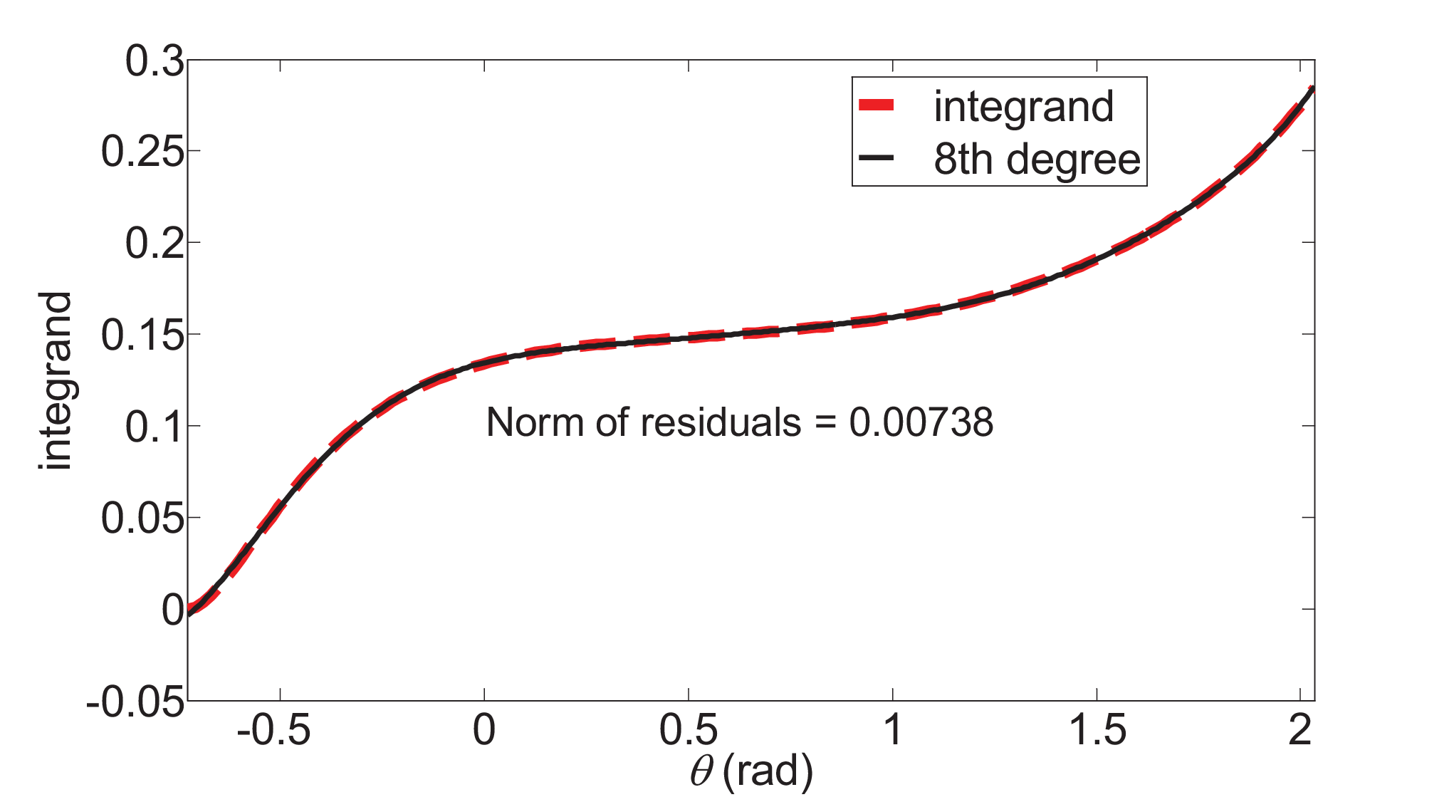
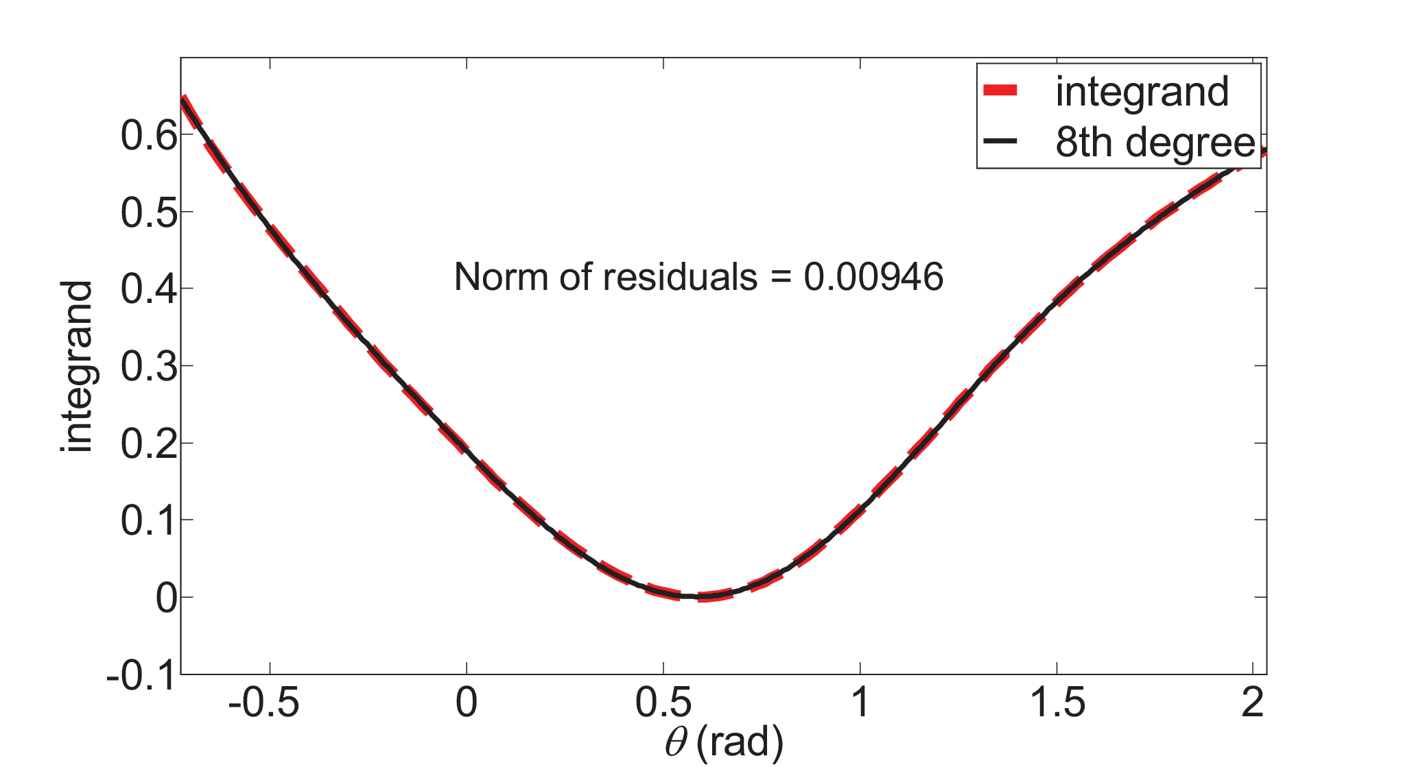
The effects of the two transformations in sub-sections 4.1 and 4.2 are demonstrated in Fig. 6. It can be seen that after the transformations, the integrands become more regular and can be well approximated by polynomials of order 8, which means that low order Gaussian quadratures can achieve accurate results.

Consider the evaluation of the regular one dimensional integral $I_{2}$ in Eq. (16), i.e., $I_{2}=\sum_{j=1}^{3}I^{(j)}_{2}$ and

One notes that the integrand of $I_{2}$ suffers from the same difficulties as that of the double integral $I_{1}$ as stated in section 3.2. The above proposed transformations can also be used to promote the efficiency of the numerical quadratures.

In this section close form expression for $I_{2}$ is derived. It is attributed to the fact that after the conformal transformation in section 4.1 the denominators of $f_{i}$, i.e. $A(\theta)$, become constant. For Burton-Miller equation, it is readily to see from (48) that $f_{-2}(\theta)$ is constant on each sub-triangle thanks to the constant $A(\theta)$, and that $f_{-1}(\theta)$ is typically made up of combinations of elementary trigonometric functions of $\theta$ [8]

The coefficients $c_{i}$ and $d_{i}$ are given in (49). Here we notice that the expressions in (49) are also applicable for Laplace equations. For other problems, such as elasticity, Stokes flow, the expressions of $f_{-2}$ and $f_{-1}$ are more complicated and can be derived analogously as in A.

To further simplify the derivation, the coordinate system $(\eta_{1},\eta_{2})$ is rotated so that the axis $o\eta_{1}$ is parallel to the perpendicular line of the side of $\bar{\Delta}$. Thus $\theta=\bar{\theta}$ over each sub-triangle. By substituting $\hat{\rho}(\theta)$, $f_{-2}$ and $f_{-1}$ into (35), the integral with $f_{-2}$ becomes

The integral with $f_{-1}$ consists of terms

and

The explicit expressions of integral (37) can be easily obtained and are omitted. Here the expression of $\bar{I}_{i}$ is derived. By changing the integral variable

one obtains

where,

The accuracy, effectiveness and robustness of the method in this paper are investigated. The integrals is performed over a curved element extracted from a cylinder surface. The size of the cylinder and the element are given in Fig.7. Distance $s$ in Fig. 7 is designed to change the aspect ratio of the element. $s=0.5$ represents a quite regular element; the quality of the element becomes bad as the increase of $s$. Four positions for the field point $\mathbf{x}$ are considered, which correspond to intrinsic coordinates (a) $\bm{\xi}=(0.3,0.3)$, (b) $\bm{\xi}=(0.1,0.8)$, (c) $\bm{\xi}=(0.45,0.45)$, (d) $\bm{\xi}=(0.64,0.31)$, respectively. One should note that points (b) and (c) match approximately with the nodes of the $2$th order Nyström discretization, while (d) match with that of the $3$th order. In addition, for the rather centered point (a) the original Guiggiani’s method in section 3.1 are believed to work well.

Since no analytical solutions are available, the (relative) error, given by

is evaluated by comparison with the results $I_{\text{ref}}$ of the Guiggiani’s methods using Gauss quadratures with $256$ quadrature points in angular direction and $32$ points in radial direction. $I_{\text{calc}}$ denotes the result calculated by the various methods. The single layer operator $\mathcal{S}$ and the hypersingular operator $\mathcal{H}$ are tested. The parameter $m$ in sigmoidal transformation takes the value of $3$ in weakly singular case and $2$ in hypersingular case. The basis function $\phi$ is selected as the second order monomial $\xi_{2}^{2}$.

A description of the methods tested are listed in table 2. The method in this paper are indicated by “Present” in which the line integral $I_{2}$ in (16) is computed by Gauss quadratures; while in “Present+a” the line integral is computed by using the closed formulations in section 4.3. Note that “Present+a” only validates for hypersingular integrals.

The overall performance of the present integration method is tested by incorporating it into a Nyström BEM code for solving the Burton-Miller equation. The geometry of the problem consists of three sections of cylinders, as shown in Fig. 9. The origin of coordinate system lies on the middle point of the symmetry axis of the cylinder. All the surfaces of the cylinder vibrate with given velocity $q(\mathbf{x})=\partial u/\partial\mathbf{x}$ (Neumann problem), where $u$ is chosen to be the fundamental solution $u(\mathbf{x})=G(\mathbf{x},\mathbf{y})$ in (3) with $\mathbf{y}=(0,0,0)$.

References

- [1] L. F. Canino, J. J. Ottusch, M. A. Stalzer, et al. Numerical solution of the Helmhotz equation in 2D and 3D using a high-order Nyström discretization. Journal of computational physics, 146 (1998), 627-633.
- [2] S. Rjasanow, L. Weggler. ACA accelerated high order BEM for maxwell probelms. Computational mechanics, 51 (2013), 431-441.
- [3] J. Bremer, Z. Gimbutas. A Nyström method for weakly singular integral operators on surfaces. Journal of computational physics, 231 (2012), 4885-4903.
- [4] X. W. Gao, T. G. Davies. Boundary Element Programming in Mechanics. Cambridge University Press (ISBN: 052177359-8), 2002.
- [5] D. J. Willis, J. Peraire, J. K. White. A quadratic basis function, quadratic geometry, high order panel method. In 44th AIAA Aerospace sciences meeting, number AIAA-2006-1253, 2006.
- [6] H. J. Wu, Y. J. Liu, W. K. Jiang. A low frequency fast multiploe boundary element method based on analytical integration of the hypersingular integral for 3D acoustic problems. Engineering analysis with boundary elements, 37 (2013), 309-318.
- [7] S. N. Fata. Explicit expressions for 3D boundary integrals in potential theory. International journal for numerical methods in engineering, 78 (2009), 32-47.
- [8] M. Guiggiani, G. Krishnasamy, T. J. Rudolphi, F. J. Rizzo. A general algorithm for the numerical solution of hypersingular boundary integral equations. ASME Journal of applied mechanics, 59 (1992), 604-614.
- [9] S. Järvenpää, M. Taskinen, P. Ylä-Oijala. Singularity extraction technique for integral equation methods with higher order basis functions on plane triangles and tetrahedra. International journal for numerical methods in engineering, 58 (2003), 1149-1165.
- [10] P. Kolm, V. Rokhlin. Numerical quadratures for singular and hypersingular integrals. Computers and Mathematics with Applications, 41 (2001), 327-352.
- [11] R. D. Graglia. G. Lombardi. Machine precision evaluation of singular and nearly singular potential integrals by use of Gauss quadrature formulas for rational functions. IEEE transactions on antennas and propagation, 56 (2008), 981-998.
- [12] M. Carley. Numeriacl quadratures for singular and hypersingular integrals in boundary element methods. SIAM journal on scientific computing, 29 (2007), 1207-1216.
- [13] M. A. Khayat, D. R. Wilton, P. W. Fink. An improved transformation and optimized sampling scheme for the numberical evaluation of singular and near-singular potentials. IEEE transactions on antennas and propagation, 7 (2008), 377-380.
- [14] M. A. Khayat, D. R. Wilton. Numerical evaluation of singular and near-singular potential integrals. IEEE transactions on antennas and propagation, 53 (2005), 3180-3190.
- [15] M. G. Duffy. Quadrature over a pyramid or cube of integrands with a singularity at a vertex. SIAM Journal on Numerical Analysis, 19(6): 1260-1262, 1982.
- [16] B. M. Johnston, P. R. Johnston. A comparsion of transformation methods for evaluating two-dimensional weakly singular integrals. International journal for numerical methods in engineering, 56 (2003), 589-607.
- [17] L. Scuderi. On the compuation of nearly singular integrals in 3D BEM collocation. International Journal for numerical methods in engineering, 74 (2008), 1733-1770.
- [18] K. Hayami. Variable transformation for nearly singular integrals in the boundary element method. Research institute for mathematical sciences, Kyoto university, 41 (2005), 821-842.
- [19] B. M. Johnston, P. R. Johnston, D. Elliott. A new method for the numerical evaluation of nearly singular integrals on triangular elements in the 3D boundary element method. Journal of Computational and Applied Mathematics, 245 (2013), 148-161.
- [20] A. J. Burton, G. F. Miller. The application of integral equation methods to the numerical solution of some exterior boundary-value problems. Proceedings of the Royal Society of London, Series A, 323 (1971), 201-210.
- [21] X. W. Gao. An effective method for numerical evaluation of gneral 2D and 3D high order singular boundary integrals. Computer methods in applied mechanics and engineering, 199 (2010), 2856-2864.
- [22] P. R. Johnston. Application of sigmoidal transformations to weakly singular and near-singular boundary element integrals. International journal for numerical methods in engineering, 45 (1999), 1333-1348.
- [23] C. Schwab, W. L. Wendland. Kernel properties and representations of boundary integral operators. Mathematische Nathrichten, 156 (1992), 187-218.