Interacting Particle Systems in Time-Dependent Geometries

Consider an isotropic radial structure with initial radius $r_{0}$ as shown in Figure 1(a), which is a particular example of radially annihilating Brownian motion. We consider directed radial growth where each arm of the displacement along the perimeter of the growing circle can be represented as a function of the radial distance $r$,

$$(Y_{r},r\geq r_{0})\quad\mbox{with}\quad Y_{r}\in[0,2\pi r)\ .$$

Increments of this process

$$dY_{r}=Y_{r}\,dr/r+d\tilde{Y}_{r}$$

(1)

are given by a contribution due to the stretching of space, and a second one due to the inherent fluctuations encoding the local scale invariance of the arms. We use this notation for increments on a formal, heuristic level in this section, which is made mathematically precise in Section 3. In the analogous fixed domain geometry Figure 1(b), we model a single arm of the same growth structure as a process

$$(X_{h},h\geq 0)\quad\mbox{with}\quad X_{h}\in[0,L)\ ,$$

for which the increments are simply given by fluctuations $dX_{h}$. In order to connect the two domains we take $r_{0}=L/2\pi$ and have periodic boundary conditions at the edges. With matching the initial conditions $X_{0}=Y_{r_{0}}$ this implies

$$X_{h}=\frac{r_{0}}{r}Y_{r}\ ,$$

(2)

in analogy to the usual polar coordinated transformation. The displacement of the rescaled radial arm has the same range as the fixed arm, and using (1) we get for the increments

$$dX_{h}=\frac{r_{0}}{r}d\tilde{Y}_{r}\ .$$

(3)

In each geometry the arms share the same local scale invariance property, i.e. the increments due to fluctuations scale as

$$dX_{h}\sim(dh)^{\gamma}\quad\mbox{and}\quad d\tilde{Y}_{r}\sim(dr)^{\gamma},$$

(4)

where $\gamma>0$ and proportionality constants in both cases are the same. Generic examples are self-similar processes where $(X_{bh},h\geq 0)$ is distributed as $(b^{\gamma}X_{h},h\geq 0)$ for all $b>0$, such as fractional Brownian motion [29], or $\alpha$-stable Lévy processes [30], which will be discussed in Section 3 in more detail.

From (4) and (3) we get heuristically

$$\frac{dh}{dr}=\Big(\frac{dx}{dy}\Big)^{1/\gamma}=\Big(\frac{r_{0}}{r}\Big)^{1/\gamma},$$

and therefore

$$h(r)=\int_{r_{0}}^{r}\Big(\frac{r_{0}}{s}\Big)^{1/\gamma}ds=\left\{\begin{array}[]{cl}\frac{\gamma}{1-\gamma}\,r_{0}\Big[1-\big(\frac{r_{0}}{r}\big)^{\frac{1-\gamma}{\gamma}}\Big]&,\ \gamma\neq 1\\ r_{0}\log\big(\frac{r}{r_{0}}\big)&,\ \gamma=1\end{array}\right..$$

(5)

For a single arm matching the initial condition $Y_{r_{0}}=X_{0}$ leads to the identical distribution

$$\Big(\frac{r_{0}}{r}\,Y_{r},r\geq r_{0}\Big)\stackrel{{\scriptstyle\mathrm{dist.}}}{{=}}\big(X_{h(r)},r\geq r_{0}\big),$$

(6)

Crucially, the same holds for the entire growth structure which are characterized as a collection of arms $\{(Y_{r},r\geq r_{0})\}$ and $\{(X_{h},h\geq 0)\}$:

$$\Big\{\Big(\frac{r_{0}}{r}\,Y_{r},r\geq r_{0}\Big)\Big\}\stackrel{{\scriptstyle\mathrm{dist.}}}{{=}}\Big\{\big(X_{h(r)},r\geq r_{0}\big)\Big\}\ ,$$

(7)

provided that the arms interact locally in a scale independent way. Examples of such interactions include coagulation, annihilation or exclusion, and extensions to non-local interactions are discussed in Section 5. Figure 1 illustrates the correspondence given by the mapping for annihilating Brownian motion, where the red dashed line indicates where the marginal distributions of the two structures are equal. Note that in the above formulation equivalence holds for the full trajectories including time correlations. This will be confirmed rigorously in Section 3 for Markovian models, and a weaker corrected version will be derived for a non-Markovian example.

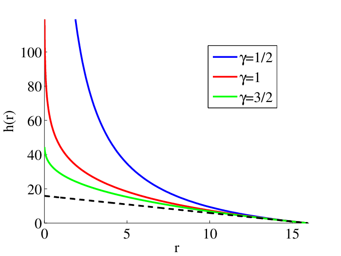
Figure 2 shows the mapping function (5) for several values of $\gamma$. For $r\rightarrow r_{0}$ we have $h(r)\simeq r-r_{0}$ for all $\gamma>0$, so that initially there is no effect on the particles from the expanding domain, since for $r$ close to $r_{0}$, the fixed and the radial domain are locally equivalent. The non-linear behavior of $h(r)$ encodes the effect of the expanding geometry the large $r$ behaviour is

$$h_{\gamma}(\infty)=\lim_{r\rightarrow\infty}h(r)=\left\{\begin{array}[]{cl}\frac{\gamma}{1-\gamma}r_{0}&,\ \gamma<1\\ \infty&,\ \gamma\geq 1\end{array}\right..$$

(8)

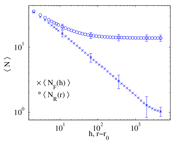
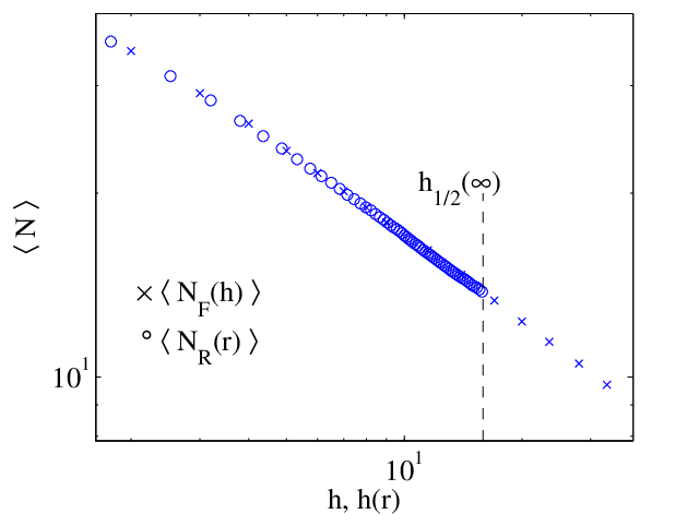
The value $h_{\gamma}(\infty)$ corresponds to the height at which the fixed width structure is equivalent to the infinite radius behaviour of the rescaled radially growing structure (see Figure 1). This asymptotic behaviour depends on the value of $\gamma$, and for $\gamma<1$ will differ from the analogous asymptotic behaviour in the fixed domain. For fixed domain structures fixation always occurs for interactions such as coagulation or annihilation, i.e. the system will eventually reach an absorbing state, as shown in Figure 3(a).

Coalescing or annihilating structures in the fixed domain $[0,L)$ are observed e.g. in neutral models for competition in spatial populations (see [4, 8, 12, 31] for more details). The fixation time $\tau$ to reach the absorbing state scales with the size $L$ of the system, where by standard arguments

$$\tau\sim L^{1/\gamma}\sim r_{0}^{1/\gamma}.$$

For large systems ($L\rightarrow\infty$), typically $\tau$ is much larger then $h_{\gamma}(\infty)\sim r_{0}$, leading to a non-trivial limit for the statistics of the radial process. This is because for structures with $\gamma<1$, the spatial expansion rate which is linear in $r$ dominates the lateral spread of random wandering of the particles, where due to the increasing distance, eventually the particles no longer interact. So the statistics for these sub-ballistic structures no longer change and reach an asymptotic value which is random, as indicated by the non-zero and $r$-independent standard deviation in Figure 3(a). In fact the whole rescaled structure converges to a non-trivial limit where

$$\Big\{\frac{r_{0}}{r}Y_{r}\Big\}\stackrel{{\scriptstyle\mathrm{dist.}}}{{\rightarrow}}\big\{X_{h_{\gamma}(\infty)}\big\}\quad\mbox{as}\quad r\rightarrow\infty.$$

For structures with $\gamma\geq 1$, the particle motion is equivalent to a (super-)ballistic trajectory exceeding the spatial expansion, where from (8) we have $h_{\gamma}(\infty)=\infty$. Here, despite the continuous expansion in space, the asymptotic behaviour for the rescaled radial process will be the same as the analogous behaviour in the fixed domain and we have

$$\Big\{\frac{r_{0}}{r}Y_{r}\Big\}\stackrel{{\scriptstyle\mathrm{dist.}}}{{\rightarrow}}\big\{X_{\infty}\big\}\quad\mbox{as}\quad r\rightarrow\infty.$$

We can also express the mapping (5) independently of the system size. Introducing dimensionless variables $r^{\prime}=r/r_{0}$ and $h^{\prime}=h/r_{0}$ leads to

$$h^{\prime}(r^{\prime})=\left\{\begin{array}[]{cl}\frac{\gamma}{1-\gamma}\left(1-\left(1/r^{\prime}\right)^{\frac{1-\gamma}{\gamma}}\right)&,\ \gamma\neq 1\\ \log r^{\prime}&,\ \gamma=1\end{array}\right.\ ,$$

(9)

for all $r^{\prime}\geq 1$, where for $\gamma=1$ we recover the generic conformal map from the exterior of the unit circle to a strip. This notation shows that $r_{0}$ plays merely the role of a length scale and $\gamma$ is the only important parameter of the mapping. Moreover, (9) takes the form of a generalized q-logarithm [32], which can therefore be seen as a generic generalization of the standard conformal map in this context.

Consider a standard Brownian motion $B:=(B_{t},t\geq 0)$, which is a centered Gaussian process with mean $\langle B_{t}\rangle=0$ and covariance

$$\langle B_{t}B_{s}\rangle=\mathrm{min}(t,s)\ ,$$

and is self similar and locally scale invariant with $\gamma=1/2$. In this case we can give a rigorous derivation of the mapping $h(r)$ using Itô-calculus. Consider the arms $X:=(X_{h},h\geq 0)$ and $Y:=(Y_{r},r\geq r_{0})$ as defined in Section 2. The corresponding Langevin equations in standard notation of stochastic differential equations are [33],

$$dX_{h}=dB_{h}$$

(11)

and

$$dY_{r}=Y_{r}\,dr/r+dB_{r}.$$

(12)

The first term in (12) corresponds to the stretching of space which is proportional to the angular displacement $Y_{r}/r$, the second term in (12) describes the inherent fluctuations of the process, where $dB$ denotes infinitesimal increments of a standard Brownian motion. For the rescaled process

$$Z:=(Z_{r},r\geq 0)\quad\mbox{with}\quad Z_{r}=\frac{r_{0}}{r}\,Y_{r}\,,$$

(13)

using Itô’s formula we have

$$dZ_{r}=\frac{r_{0}}{r}\,dB_{r}.$$

(14)

In integral form this implies $Z_{r}=\int_{r_{0}}^{r}r_{0}/s\,dB_{s}.$ It is well known that this stochastic Itô integral can be written as a time-changed Brownian motion so that the process $Z$ is a continuous time martingale, where $Z_{r}=B_{h(r)}$. The time change is given by the quadratic variation of $Z$

$$h(r)=\int_{r_{0}}^{r}\Big(\frac{r_{0}}{s}\Big)^{2}\,ds=r_{0}\Big(1-\frac{r_{0}}{r}\Big)\ .$$

(15)

The quadratic variation basically describes the accumulated mean squared displacement up to time $t$, and is simply equal to $t$ for standard Brownian motion. In general, every Itô integral with respect to Brownian motion such as $Z_{r}$ is a martingale, and can be written as a time-changed Brownian motion using the above formula (see e.g. [33] page 56 for details). This gives a rigorous justification of the mapping (5) for Brownian motion with $\gamma=1/2$ and equivalence in the strong sense (6), i.e. the full process including time correlations is mapped correctly.

Structures where the position of the arms exhibit super-diffusive behaviour due to jumps in their trajectories can be modelled by $\alpha$-stable Lévy processes [34, 35]. A stochastic process $L=(L^{\alpha}_{t},t\geq 0)$, with $\alpha\in(0,2)$ is an $\alpha$-stable Lévy process if it has stationary independent increments and a pdf $p_{\alpha}(x,t)$ whose Fourier transform takes the form

$$\hat{p}_{\alpha}(k,t)=\exp(-\sigma_{\alpha}t|k|^{\alpha}/2).$$

(16)

Lévy Processes are Markovian with discontinuous paths, they have increments with infinite variance, and for $\alpha\in(0,1)$ their absolute first moment is also infinite. Another key property is that the fractional moments of $L^{\alpha}_{t}$ scale as

$$\langle|L^{\alpha}_{t}|^{q}\rangle=(\sigma_{\alpha}t^{1/\alpha})^{q},$$

(17)

where $0<q<\alpha$ is non-integer [30, 34]. In practice, the parameter $\alpha$ can be greater then $2$, but in this case the increments have a finite mean and variance, and such a process scales diffusively.

When the arms $X$ and $Y$ are $\alpha$-stable Lévy processes, through a generalization of Itô calculus, [30, 36], the rescaled process $Z$ can be expressed in Langevin form as

$$dZ_{r}=\frac{r_{0}}{r}\,dL^{\alpha}_{r}.$$

(18)

The process $Z$ is also a time-changed $\alpha$-stable Lévy process (see [36], page 237). By using the property (17) on (18) we can match all $q$-moments of $dX$ and $dZ$,

$$(c_{\alpha}dh)^{q/\alpha}=\Big(\frac{r_{0}}{r}\Big)^{q}(c_{\alpha}dr)^{q/\alpha},$$

provided that

$$h(r)=\int_{r_{0}}^{r}\Big(\frac{r_{0}}{s}\Big)^{\alpha}\,ds\ ,$$

which is the mapping (5) with $\gamma=1/\alpha$. Therefore the process $Z_{r}$ is an $\alpha$-stable Lévy process $L^{\alpha}_{h(r)}$ and the result holds in its strong form (6). Note that for $\alpha\geq 2$ Lévy processes scale like Brownian motion and do not become subdiffusive, so that for general $\alpha>0$ we have $\gamma=\mathrm{max}\{1/\alpha,1/2\}$.

Figure 4(a) shows the expected number of particles $\langle N_{F}(h)\rangle$ and $\langle N_{R}(r)\rangle$, plotted against $h$ and $h(r)$, respectively, for several values of $\alpha$ under coalescing dynamics. The figure shows that we have a very good data collapse, where the radial data converges to $\langle N_{F}(h_{\gamma}(\infty))\rangle$ as explained in Section 2.2. Being Markov processes with independent increments, we can simulate Lévy processes simply by adding independent increments. We take the absolute value of each increment $dL^{\alpha}$ to be distributed by the Pareto distribution with pdf

$$p_{\alpha}(x)=\alpha b^{\alpha}/x^{\alpha+1}\quad\mbox{for}\quad x\geq b,$$

(19)

where $b=dt^{1/\alpha}$ with $dt$ being the simulation time-increment. Taking $dt\ll 1$ small we reproduce data which is consistent with the infinitesimal limit $dt\rightarrow 0$, and therefore we simulate good approximations of sample paths of $\alpha$-stable Lévy processes [30]. Coalescence or annihilation interaction can easily be implemented even for discontinuous paths with discrete time sampling, since in one space dimension every event can be detected by a change of the particle order. We do not include multiple coalescence events, i.e. if a particle jumps across several others, we just coalesce it with the nearest one at the position of the latter.

The long time behaviour in the fixed domain can be computed analytically (see A.2), where in a scaling window of intermediate $h$

$$\langle N_{F}(h)\rangle=L/(\pi\sigma_{\alpha}h^{2/\alpha})^{1/2},$$

(20)

and this is shown by the black dashed line in Fig. 4a. Using (20) and (8) the corresponding asymptotic behaviour for the radial structure is

$$\langle N_{R}(r)\rangle\rightarrow\left\{\begin{array}[]{cl}2\sigma_{\alpha}^{-1}\pi^{1/2}\Big(\frac{r_{0}^{1-\alpha}}{\alpha-1}\Big)^{-1/\alpha}&,\ \alpha>1\\ 1&,\ \alpha\leq 1\end{array}\right.\quad\mbox{as}\quad r\rightarrow\infty$$

(21)

and this limit is indicated for the $\alpha=3/2$ data by the red dashed lines, where the values for $\sigma_{\alpha}\approx 1.4$, $4$ and $10.8$ for $\alpha=1,$ $3/2,$ and $5/2$ respectively, are fitted to the data.

Figure 4(b) shows the corresponding behaviour of $\langle D^{2}\rangle$ as defined in (10). Both $\langle D_{F}^{2}\rangle$ and the $\langle D_{R}^{2}\rangle$ are increasing functions, and in the fixed domain $\langle D_{F}^{2}(h)\rangle$ will converge to $L^{2}$. For the radial domain the rescaled behaviour $\langle(r_{0}D_{R}(r)/r)^{2}\rangle$ is shown, where by plotting against $h(r)$ we attain a data collapse.

We also consider structures where the displacement of the arms perform fractional Brownian motion (fBm) [29, 37]. The fBm $B^{H}=(B^{H}_{t},t\geq 0)$ with Hurst exponent $H\in(0,1)$ is a centered Gaussian process with continuous paths and covariance

$$\langle B^{H}_{t}B^{H}_{s}\rangle=\frac{1}{2}(t^{2H}+s^{2H}-|t-s|^{2H})\ .$$

(22)

In particular, $\langle(B^{H}_{t})^{2}\rangle=t^{2H}$, the pdf of $B_{t}^{H}$ takes the general form

$$p(x,t)=\frac{1}{\sqrt{2\pi t^{2H}}}\exp\Big(-\frac{x^{2}}{2t^{2H}}\Big)$$

(23)

and the process exhibits local scale invariance (4) with $\gamma=H$. When $H=1/2$, the process is a Brownian motion as in Section 3.1, and for $H\neq 1/2$ the process is not Markovian since it has long range temporal correlations [29]. When the arms are fBm as before the rescaled process (14) can be written in integral form as

$$Z_{r}=\int_{r_{0}}^{r}\frac{r_{0}}{s}\,dB^{H}_{s}.$$

(24)

For $H\neq 1/2$ this integral w.r.t fBm cannot be written as a time-changed fBm [38], so the mapping does not hold in its strong form (6). This is due to memory effects coming from the non-Markovian correlated noise $dB_{t}^{H}$ leading to non-independent increments. Nevertheless, using fractional calculus we can compute and match the second moment of the rescaled radial process and the fixed process $B^{H}$. We represent $Z_{r}$ in (24) as a memory kernel integral with respect to a standard Brownian motion (see [29] page 48), leading to the following representation:

$$Z_{r}=\int_{r_{0}}^{r}\Big(K^{*}_{H}\frac{r_{0}}{(\cdot)}\Big)(s)dB_{s}.$$

(25)

The operator $K_{H}$ and further details are given in B. In the form given in (25), we match the quadratic variations of $Z_{r}$ with $X_{h_{H}(r)}$ to obtain

$$h_{H}(r)=\Big[H(2H-1)\int_{r_{0}}^{r}\int_{r_{0}}^{r}\frac{r_{0}^{2}}{xy}|x-y|^{2H-2}dxdy\Big]^{1/2H}.$$

(26)

This can also be written using hypergeometric functions

	$\displaystyle h_{H}(r)=\Bigg[Hr_{0}^{2}\int_{0}^{r-r_{0}}\Big[$	$\displaystyle\frac{(r-r_{0}-y)^{-1+2H}{}_{2}F_{1}\left[1,-1+2H,2H,\frac{r_{0}-r+y}{r_{0}+y}\right]}{(r_{0}+y)^{2}}+$			(27)
		$\displaystyle\frac{y^{-1+2H}{}_{2}F_{1}\left[1,1,2H,-\frac{y}{r_{0}}\right]}{r_{0}(y+r_{0})}\Big]dy\Bigg]^{1/2H}\,.$

This second representation also holds for $H=1/2$, where it simplifies to (15). Note that although for $H\neq 1/2$ the expression of (26) differs from (5), visual comparisons as plotted in Figure 5(a) for $H=1/3$ and $H=2/3$ shows that they are very close. In fact, for the rest of this paper (especially Figs. 6 and 9) we do not distinguish between the two mappings. However, for fBm we are only able to match first and second moment of the processes $Z_{r}$ and $X_{h(r)}$, and the equivalence in the form (6) does not hold. Since Gaussian random variables are uniquely determined by their first and second moment, we still have

$$\Big\{\frac{r_{0}}{r}Y_{r}\Big\}\stackrel{{\scriptstyle\mathrm{dist.}}}{{=}}\big\{X_{h(r)}\big\}\quad\mbox{for all}\quad r\geq r_{0}\ ,$$

i.e. equivalence for all marginals but not for the time correlations. The behaviour for small radius $r\in[r_{0},r_{0}+\epsilon]$ using (26) is

	$\displaystyle\lim_{\epsilon\rightarrow 0}\frac{h_{H}(\epsilon+r_{0})}{\epsilon}$	$\displaystyle=$	$\displaystyle\lim_{\epsilon\rightarrow 0}\bigg[H(2H-1)\int_{0}^{1}\int_{0}^{1}\frac{r_{0}^{2}|x-y|^{2H-2}}{(r_{0}+\epsilon x)(r_{0}+\epsilon y)}dxdy\bigg]^{1/2H}$
		$\displaystyle=$	$\displaystyle\Big[H(2H-1)\int_{0}^{1}\int_{0}^{1}|x-y|^{2H-2}dxdy\Big]^{1/2H}=1.$

So $h(r)\simeq r-r_{0}$ for $r$ close to $r_{0}$. Note that (26) and (5) will mostly differ when $r$ is large (see Figure 5(b)), where in the limit as $r\rightarrow\infty$ we have

	$\displaystyle\lim_{r\rightarrow\infty}h_{H}(r)$	$\displaystyle=$	$\displaystyle r_{0}\Big[H(2H-1)\int_{0}^{\infty}\int_{0}^{\infty}\frac{|x-y|^{2H-2}}{(x+1)(y+1)}dxdy\Big]^{1/2H}$		(28)
		$\displaystyle=$	$\displaystyle r_{0}\pi^{\frac{1}{2H}}\left(\frac{H(2H-1)}{(H-1)\sin(2\pi H)}\right)^{\frac{1}{2H}}.$

Comparing this value to (8) we have

$$h_{H}(\infty)=\lim_{r\rightarrow\infty}h_{H}(r)\quad\left\{\begin{array}[]{cl}=h_{\gamma}(\infty)=\frac{\gamma}{1-\gamma}\,r_{0}&,\ H=1/2\\ <h_{\gamma}(\infty)=\frac{\gamma}{1-\gamma}\,r_{0}&,\ H\neq 1/2\end{array}\right..$$

(29)

Figure 6 shows the statistics $\langle N\rangle$ and $\langle D^{2}\rangle$ for radially expanding and fixed fBm structures. Since fBm is non-Markovian, sample paths cannot be generated by adding increments that depend only on the current state. The easiest way to generate a discretized sample of an fBm path at times $t_{1},\ldots,t_{n}$ which we implemented, is to invert the covariance matrix $\langle B^{H}_{t_{i}}B^{H}_{t_{j}}\rangle$ given by (22) and multiply with a vector of iid Gaussian increments (cf. [29] Section 10 for details). For the radially expanding structure we use the mapping (5) with $\gamma=H$ and plot $\langle N_{R}(r)\rangle$ vs $h(r)$. This gives a good data collapse despite as shown above this is strictly not the correct mapping. Figure 6(b) shows the behaviour of $\langle D^{2}\rangle$. This follows similar behaviour to the Lévy data [as seen in Figure 4(b)]. Again by plotting the rescaled $\langle(r_{0}D_{R}(r)/r)^{2}\rangle$ against $h(r)$ we have a data collapse. For fBm the full behaviour of $\langle N_{F}(h)\rangle$ and $\langle D_{F}(h)^{2}\rangle$ can be analytically approximated (see A.1) which is shown by the full black lines.

As we have seen before, the mapping (5) is unique for all locally scale invariant Markovian models. However, there are many other self-similar systems which are not locally scale invariant, for which similar but different mappings can be derived rigorously. Here we focus on a special example of Brownian motion with time dependent diffusion coefficient. For such processes the equations governing the fixed and radial process are

$$dX_{h}=\phi(h)dB_{h}$$

(30)

and

$$dY_{r}=Y_{r}\,dr/r+\phi(r-r_{0})dB_{r}.$$

(31)

Here $B$ is taken to be a standard Brownian motion with exponent $\gamma=1/2$. The function $\phi:[0,\infty)\rightarrow[0,\infty)$ is a continuous positive function, some interesting forms of $\phi$ are power laws such that $\phi(t)\sim t^{\delta}$. Such a function can be seen to occur for biologically motivated models as in [12] and are also observed in DLA structures [27]. In this case we have

$$\langle X_{h}^{2}\rangle\sim\int_{0}^{h}s^{2\delta}ds\sim h^{2\delta+1}\ ,$$

and we consider $-1/2<\delta<1/2$ which leads to sub- and superdiffusive processes with Hurst exponent $\frac{1}{2}+\delta$. Treating these processes as before, the rescaled process (13) can be seen to satisfy

$$dZ_{r}=(r-r_{0})^{\delta}\frac{r_{0}}{r}\,dB_{r}\ .$$

(32)

Taking the fluctuations in (30) and (32) to satisfy (4) and using the fact that the rescaled process has the same law as the process in the fixed domain leads to the following relationship between the temporal coordinates $(h,r)$

$$h_{\delta}(r)=\left[(1+2\delta)\int_{r_{0}}^{r}\Big(\frac{r_{0}}{s}\Big)^{2}(s-r_{0})^{2\delta}\,ds\right]^{\frac{1}{2\delta+1}}\ .$$

This can also be written as

	$\displaystyle h_{\delta}(r)$	$\displaystyle=\Bigg[(1+2\delta)r_{0}^{2}\Gamma\Big(1-2\delta\Big)\Bigg[r_{0}^{-1+2\delta}\,\Gamma\Big(2\delta+1\Big)-$			(33)
		$\displaystyle\qquad{}r^{-1+2\delta}\,{}_{2}F_{1}\left[-2\delta,1-2\delta,2-2\delta,\frac{r_{0}}{r}\right]\Bigg]\Bigg]^{1/(2\delta+1)},$

where $\Gamma(\cdot)$ is the gamma function. Thus the mapping (33) complements the one for locally scale invariant structures (5), applying to a different class of self-similar processes and resulting stochastic structures. For $-1/2<\delta<1/2$ (33) has the finite limit

$$h_{\delta}(\infty)=\Bigg[(1+2\delta)r_{0}^{2\delta+1}\Gamma\Big(1-2\delta\Big)\Gamma\Big(1+2\delta\Big)\Bigg]^{1/(1+2\delta)}.$$

(34)

In Figure 7 we compare both mappings (5) and (33). We take the parameter $\delta$ such that $\gamma=1/2+\delta$, this equates the exponent of the mean squared displacement for each arm in their respective system. In Figure 7(a) we see that despite initial similarity, for larger values of $r$ both mappings converge to clearly different limits, as is illustrated in Figure 7(b). This difference is far clearer than differences between (5) and the mapping for fBm processes (26), and shows that processes with the same mean squared displacements cannot necessarily be mapped by similar functions. Note also that by construction $X_{h}$ (30) and the rescaled process $Z_{r}$ (32) are time-changed Brownian motions in this example, and therefore the mapping holds in its strong form (6).

We start by considering decreasing radial structures where the length of the domain decreases uniformly as a function of the radius. This particular geometry has received attention in [21] for competition interfaces in the Eden growth model, which is in the Kardar-Parisi-Zhang universality class and the competition interface has been shown to be scale invariant with $H=2/3$ see [4, 12, 13, 39]. More recently decreasing domains have also been studied in [31] under the assumption of diffusive domain boundaries, and our general approach includes both cases. Figure 8(a) shows an illustration of such a coalescing structure, where particles diffuse with $\gamma=1/2$ on a decreasing radial domain. We can easily adapt the mapping $h(r)$ to take into account the decreasing radius, where (5) becomes

$$h(r)=\int_{r}^{r_{0}}\Big(\frac{r_{0}}{s}\Big)^{1/\gamma}ds=\left\{\begin{array}[]{cl}\frac{\gamma r_{0}}{1-\gamma}\left[(\frac{r_{0}}{r})^{\frac{1-\gamma}{\gamma}}-1\right]&,\ \gamma\neq 1\\ r_{0}\log(\frac{r_{0}}{r})&,\ \gamma=1\end{array}\right.,$$

(35)

where $r_{0}$ is the initial radius. The function (35) is shown in Figure 8(b), the initial behaviour is $h(r)\simeq r_{0}-r$ and as $r\rightarrow 0$ the limit depends on $\gamma$.

Comparing the mapping for inward growing structures (35) to outward growing structures (5) we see that (35) has a finite limit for $\gamma>1$, whereas the limit is infinite in (5), with the opposite behaviour for $\gamma<1$. Although for $\gamma>1$ (35) has a limit

$$h_{\gamma}(\infty)=\frac{\gamma}{\gamma-1}\,r_{0},$$

the structure on the fixed domain will have typically already fixated before, since for $\gamma>1$ the fixation time $\tau$ scales as

$$\tau\sim L^{1/\gamma}\ll L\sim r_{0}.$$

So the inward growing structure fixates for all $\gamma>0$. The special case of $\gamma=1$ corresponds to a mirror point where the limit in (5) and (35) stays the same.

In Figure 9 we illustrate the use of (35) for inward growing Lévy and fBm structures with $\gamma=\mathrm{max}\{1/\alpha,1/2\}$ and $\gamma=H$ respectively. Due to the decreasing size of the domain, $\langle N_{R}(r)\rangle\rightarrow 1$ as $r\rightarrow 0$ and by plotting $\langle N_{R}(r)\rangle$ against $h(r)$ we obtain a data collapse. For the value $H=2/3$, results on inward growing radial structures have been seen before in [21], our approach provides a framework to understand the behaviour in such geometries more clearly. By using the mapping the inward growing behaviour and the outward growing behaviour can be fully described by the fixed domain system.

Consider as before $X:=(X_{h},h\geq 0)$ an arm in the fixed domain, the displacement of this process lies in $[0,L(0))$ for all $h\geq 0$. Take $Y:=(Y_{t},t\geq 0)$ to be an arm in a homogeneous time dependent domain, this process will have a displacement in an evolving domain $[0,L(t))$ for all $t\geq 0$, where $L(t)$ is a general continuous function such that $L(t)>0$ for all $t\geq 0$. Note that the radially increasing/decreasing domain corresponds to $L(t)=2\pi r(t)$ with $r(t)=r_{0}\pm t$, where in the decreasing case we only consider time $t\in[0,r_{0})$. We assume as before that in each geometry the local scale invariance property (4) holds. The coordinate transformation (3) then generalizes to $x=\frac{L(0)}{L(t)}y$, leading to

$$\frac{dh}{dt}=\Big(\frac{dx}{dy}\Big)^{1/\gamma}=\Big(\frac{L(0)}{L(t)}\Big)^{1/\gamma}.$$

Therefore

$$h(t)=\int_{0}^{t}\Big(\frac{L(0)}{L(s)}\Big)^{1/\gamma}ds.$$

(36)

Analogous to (5), for $t$ close to $0$ we have $h(t)\simeq t$ and if $L(t)\gg t^{\delta}$ for some $\delta>\gamma$, then we have

$$\lim_{t\rightarrow\infty}h(t)<\infty.$$

For Brownian motion and Lévy flights the rigorous derivation of (36) is a simple extension of the approach we have shown in Sections 3.1 and 3.2, for fBm a rigorous derivation is given in B.

We use (36) to look at the behaviour of a structure evolving in an exponentially increasing domain

$$L(t)=L(0)\exp(t/c)$$

(37)

where $c>0$. Our motivation for choosing such a $L(t)$ is that we can study random walks with an exponentially decreasing jump size which has received a considerable amount of interest (see [40, 41, 42] for more details). These processes have a variety of practical applications in modelling simulated annealing [43, 44] or the displacement of quantum particles [45]. For this $L(t)$ we have

$$h(t)=c\gamma\left(1-\exp\left(-\frac{t}{c\gamma}\right)\right),$$

(38)

and subsequently $h(t)$ has the limit

$$h_{\gamma}(\infty)=\lim_{t\rightarrow\infty}h(t)=c\gamma.$$

Note that by the choice of $L(t)$ this limit does not depend on $L(0)$. In Figure 10 we illustrate the use of the mapping (38) for coalescing Brownian structures with $\gamma=1/2$. As in previous examples, the behaviour is mapped to the fixed domain by plotting $\langle N_{L(t)}(t)\rangle$ and $\big\langle\big(L(0)D_{L(t)}(t)/L(t)\big)^{2}\big\rangle$ against $h(t)$.

It is interesting to note that the general mapping (36) does not depend on the dimensions $n$ of the state space. Consider a $n+1$ dimensional structure, where in each spatial direction the displacements are $Y_{i}\in[0,L_{i}(t))$ with $L_{i}(t)>0$ for all $t\geq 0$. We can still characterize the behaviour of this $n+1$ dimensional evolving structure by mapping it to a fixed width structure where in each spatial direction the displacements $X_{i}$ are in the fixed domain $[0,L_{i}(0))$. In order to do this, we require the local scale invariance property (4) to hold in all spatial directions $i=1,\ldots,n$

$$dX_{i}\sim(dh)^{\gamma}\quad\mbox{and}\quad dY_{i}\sim(dt)^{\gamma}\,.$$

(39)

For such systems the mapping (36) stays exactly the same and will therefore map an evolving structure to a fixed width structure. It is also possible to include anisotropy in (39) where there can be a possible $i$-dependence of the multiplicative factors but $\gamma$ must be identical in all directions. This is illustrated in Figure 11(b) in Section 5 for coalescing particles of non-zero size on a growing 2-sphere.

Most real world structures exhibit a microscopic length scale, which in our representation corresponds to a non-zero particle size $d>0$; this influences the structures on small length scales [15]. Here we look at coalescing particle systems, where each particle has an isotropic shape with a diameter $d>0$. Introducing such a length scale in the interactions means that particles will now coagulate when the distance between their centers is less then $d$. As long as this is much smaller than the system size, i.e. $d\ll L$, the corrections introduced are small (see Figure 11). We include such corrections into the mapping by preserving the particle size scale in each domain relative to system size. Taking $d_{R}$ as the fixed diameter in the radial geometry, we have

$$d_{F}=\frac{r_{0}}{r(h)}d_{R},$$

(40)

where $d_{F}$ is the rescaled diameter in fixed geometry such that

$$d_{F}\rightarrow 0\quad\mbox{as}\quad h\rightarrow h_{\gamma}(\infty).$$

The function $r(h)$ in (40) is the inverse of (5) and for general $\gamma\neq 1$ it has the form

$$r(h)=r_{0}\left(1-\frac{1-\gamma}{\gamma}\,\frac{h}{r_{0}}\right)^{-\gamma/(1-\gamma)}$$

(41)

In Figure 11(a) we look at such systems for a range of diameters $d$. By using the mapping (5) with $\gamma=1/2$ we are able to map the behaviour in the radially growing structure to the fixed width structure, illustrated for $\langle N_{R}(r)\rangle$. For the fixed width structure simulations we include the data where the correction (40) is applied ($\times$) and where it is ignored ($+$). We can see that the inclusion of (40) provides an exact mapping between the two domains. The introduction of a particle size only affects the initial behaviour, where initially the distance between particles is small and due to $d>0$ more coalescing events take place. As time increases, the distance between particles increases and the behaviour becomes largely independent of $d$.

In Figure 11(b) we show that the mapping also works in $n=2$ dimensions, where using (5) we map the data of $\langle N\rangle$ from a growing sphere $S^{2}(r)$ to a fixed sphere $S^{2}(r_{0})$. As above, particles have a given diameter $d>0$ and we use the correction (40) on the fixed width structure as indicated by ($\times$) to obtain an exact data collapse as oppose to an approximation, indicated by ($+$) when (40) is not used. Note that in $2$ dimensions particles are not ordered, so in order to detect all coagulation events correctly in the simulation we have to choose increments in the particle motion small enough compared to the diameter $d$.

A similar treatment is possible for more general interactions with intrinsic time scales. Here we treat coagulating and branching structures. These structures have much interest due to a wide variety of applications, some examples include the modelling of surnames in genealogy [46], or the growth of microbial species with mutation [31]. We generalize the diffusing coalescing model studied in Section 2 by adding the mechanism of particle branching to the system. In order to map the length scale of branching correctly, which is encoded in the branching rate, we derive a relationship between the rate $R_{F}$ in the fixed domain and $R_{R}$ in the growing radial domain such that the number of branch events in each domain is equal. Let $N_{R}(\Delta r)$ be the number of branch events in the radial domain in the interval $[r,r+\Delta r]$ and let $N_{F}(\Delta h)$ correspond to the number of events in the fixed domain in the interval $[h,h+\Delta h]$. Then $R_{F}=N_{F}(\Delta h)/\Delta h$ and $R_{R}=N_{R}(\Delta r)/\Delta r$, and by using (5) and requiring $N_{F}(\Delta h)=N_{R}(\Delta r)$, we have

$$\frac{R_{R}}{R_{F}}=\frac{N_{R}(\Delta r)/\Delta r}{N_{F}(\Delta h)/\Delta h}=\frac{\Delta h}{\Delta r}=\frac{r_{0}^{2}}{r^{2}}.$$

Mostly we are interested in mapping a radial structure with fixed rate $R_{R}$ to a fixed width structure with a variable rate such that

$$R_{F}(h)=\Big(\frac{r(h)}{r_{0}}\Big)^{2}R_{R},$$

(42)

where $r(h)$ is as in (41) with $\gamma=1/2$.

We consider two types of models where particles branch. In each case the particles perform Brownian motion and coalesce upon contact, and a branch event occurs after a random time exponentially distributed with mean $1/R_{F}$ ($1/R_{R}$) for the fixed (radial) domain structure. In one model, which we call “uniform”, the new particle is placed uniformly in the domain. In the second model which we call “local” the new particle is placed in the same position as its mother. In order to avoid instantaneous coalescence between the daughter and mother particles we prohibit coalescence and both particles move independently until they have both branched again.

In Figure 12 we use the mapping (41) with the relationship (42) to map the density from the fixed domain to the growing radial domain. This shows that $\langle N_{R}(r)\rangle$ is asymptotically linear in $r$ and we can predict the speed constant. In (a) the full black line and in (b) the dashed black line correspond to the expression (46) which is an analytical prediction for the density $\rho(r)$ for the uniform model. Here we have adapted previous mean field results, [21, 24, 26], to take into account the density dependent input of particles, as explained below.

For coalescing structures in the fixed domain, when particles perform Brownian motion the one dimensional rate equation [21] governs the behaviour of the density $\rho(h)$, and reads

$$\frac{d\rho}{dh}=-\frac{\pi\rho^{3}}{2}$$

(43)

with solution $\rho(h)\sim h^{-1/2}.$ For the uniform model we adapt Eq. (43) by considering a density dependent input into the domain [26]. This leads to an additive term

$$\frac{d\rho}{dh}=-k_{1}\rho^{3}+k_{2}\rho,$$

(44)

where $k_{1}=\pi/2$ and $k_{2}=C_{2}R_{F}$ is a model dependent constant proportional to $R_{F}$. Fitting to the data we find $C_{2}\approx 0.6158$. In order to obtain an analytical expression for the growing radial domain, we modify the density equation (44) using the relation (42), which leads to

$$\frac{d\rho}{dh}=-k_{1}\rho^{3}+k_{2}\Big(\frac{r_{0}}{r_{0}-h}\Big)^{2}\rho.$$

(45)

Using (5) the solution to (45) can be written as

$$\rho(r)=\frac{e^{k_{2}r}r_{0}}{r}\Bigg[e^{2k_{2}r_{0}}+2k_{1}\Big[-e^{2k_{2}r_{0}}r_{0}^{2}/t+2k_{2}r_{0}^{2}\Phi\big(2k_{2}t\big)\Big]_{r_{0}}^{r}\Bigg]^{-1/2},$$

(46)

where $\Phi(x)=\int^{x}e^{t}/t\,dt$. For large $r$ (46) can be expressed as

$$\rho(r)\approx\frac{1}{r}\Bigg[2k_{1}\Big(-\frac{1}{r}+2k_{2}e^{-2k_{2}r_{0}}\Phi\big(2k_{2}r\big)\Big)\Bigg]^{-1/2},$$

(47)

and for $r\rightarrow\infty$

$$e^{-2k_{2}r_{0}}\Phi\big(2k_{2}r\big)\approx\frac{1}{2k_{2}r}+\frac{1}{(2k_{2}r)^{2}}+O(1/r^{3}).$$

Combining this with (47) gives

$$\lim_{r\rightarrow\infty}\rho(r)=\left(\frac{k_{2}}{k_{1}}\right)^{1/2}\approx\sqrt{\frac{C_{2}R_{R}}{\pi/2}}.$$

(48)

This limit is indicated on the right axis in Figure 12(a) and matches the data very well, along with the prediction of the full solution (46).

The validity of the rate equation is based on mean-field arguments, and it is therefore not surprising that it does not predict well the behaviour of the local model, as can be seen in Figure 12(b). However, the main point is that we still have a perfect data collapse from the mapping and can use the fixed geometry to fully understand the radially increasing domain. Other processes such as pair creation, which are relevant in mutation processes in expanding biological populations [31], can be treated in full analogy.

References

- [1] T. A. Witten and L. M. Sander. Diffusion-Limited Aggregation, a Kinetic Critical Phenomenon. Phys. Rev. Lett., 47(19):1400–1403, 1981.
- [2] H.E. Stanley, A. Bunde, S. Havlin, J. Lee, E. Roman, and S. Schwarzer. Dynamic mechanisms of disorderly growth: Recent approaches to understanding diffusion limited aggregation. Physica A, 168(1):23–48, 1990.
- [3] H.E. Stanley, A. Coniglio, S. Havlin, J. Lee, S. Schwarzer, and M. Wolf. Diffusion limited aggregation: a paradigm of disorderly cluster growth. Physica A, 205(1-3):254–271, 1994.
- [4] Y Saito and H Müller-Krumbhaar. Critical Phenomena in Morphology Transitions of Growth Models with Competition. Phys. Rev. Lett., 74(21):4325–4328, 1995.
- [5] P. G. Saffman and G Taylor. The penetration of a fluid into a porous medium or Hele-Shaw cell containing a more viscous fluid. Proc. R. Soc. Lond. A, 245(1242):312–329, 1958.
- [6] L Paterson. Radial fingering in a Hele Shaw cell. J. Fluid Mech., 113:513–529, 1981.
- [7] H Thome, M Rabaud, V Hakim, and Y Couder. The Saffman-Taylor instability: From the linear to the circular geometry. Phys. Fluids A, 1(2):224–240, 1989.
- [8] O Hallatschek, P Hersen, S Ramanathan, and D R Nelson. Genetic drift at expanding frontiers promotes gene segregation. Proc. Natl. Acad. Sci. USA, 104(50):19926–19930, 2007.
- [9] K S Korolev, M Avlund, O Hallatschek, and D R Nelson. Genetic demixing and evolution in linear stepping stone models. Rev. Mod. Phys., 82(2):1691–1718, 2010.
- [10] E Somfai and L M Sander. Scaling and river networks: A Landau theory for erosion. Phys. Rev. E, 56(1):R5–R8, 1997.
- [11] A L Barabasi and H E Stanley. Fractal concepts in surface growth. Cambridge University Press, 1st edition, 1995.
- [12] A Ali and S Grosskinsky. Pattern formation through genetic drift at expanding population fronts. Adv. Complex Syst., 13(3):349–366, 2010.
- [13] A Ali, E Somfai, and S Grosskinsky. Reproduction-time statistics and segregation patterns in growing populations. Phys. Rev. E, 85(2):021923, 2012.
- [14] A Bunde and S Havlin. Fractals and disordered systems. Springer, 2nd edition, 1995.
- [15] R Kopelman. Fractal Reaction Kinetics. Science, 241(4873):1620–1626, 1988.
- [16] W Kurz and D J Fisher. Fundamentals of Solidification. Trans Tech Publ, 1st edition, 1989.
- [17] Jacob C. Branching Processes: Their Role in Epidemiology. Int. J. Environ. Res. Public Health, 7(3):1186–1204, 2010.
- [18] J D Murray. Mathematical Biology II: Spatial Models and Biomedical Applications. Springer, 3rd edition, 2003.
- [19] B B Mandelbrot. The Fractal Geometry of Nature. W. H. Freeman, 1st edition, 1982.
- [20] R Lehe, O Hallatschek, and L Peliti. The Rate of Beneficial Mutations Surfing on the Wave of a Range Expansion. PLoS Comput. Biol., 8(3):e1002447, 2012.
- [21] N I Lebovka and N V Vygornitskii. How does the geometry affect the criticality in two-component spreading phenomena? J. Phys. A: Math. Gen., 31(46):9199–9208, 1998.
- [22] M Eden. A two-dimensional growth process. Proc. Fourth Berkeley Symposium on Maths, Statistics and Probility., 4(0):223–239, 1961.
- [23] R Munasinghe, R Rajesh, R Tribe, and O Zaboronski. Multi-scaling of the n-Point Density Function for Coalescing Brownian Motions. Commun. Math. Phys., 268(3):717–725, 2006.
- [24] P A. Alemany and D ben-Avraham. Inter-particle distribution functions for one-species diffusion-limited annihilation, . Phys. Lett. A, 206(1-2):18–25, 1995.
- [25] Kazuo S and Tomohiro N. Exact Results for a Diffusion-Limited Pair Annihilation Process on a One-Dimensional Lattice. J. Phys. Soc. Jpn., 69(5):1341–1351, 2000.
- [26] T O. Masser and D ben-Avraham. Method of intervals for the study of diffusion-limited annihilation, . Phys. Rev. E, 63(6):066108, 2001.
- [27] A Ali, R C Ball, S Grosskinsky, and E Somfai. Scale-invariant growth processes in expanding space. Phys. Rev. E, 87:020102, 2013.
- [28] I Pazsit and L Pal. Neutron Fluctuations: A Treatise on the Physics of Branching Processes. Elsevier Science, 1st edition, 2007.
- [29] F Biagini, Y Hu, B Øksendal, and T Zhang. Stochastic Calculus for Fractional Brownian Motion and Applications. Springer, Berlin, 1st edition, 2008.
- [30] A V. Chechkin, R Metzler, J Klafter, and V Y Gonchar. Introduction to the Theory of Lévy Flights. Wiley-VCH Verlag GmbH & Co. KGaA, 2008.
- [31] M O Lavrentovich, K S Korolev, and D R. Nelson. Radial domany-kinzel models with mutation and selection. Phys. Rev. E, 87:012103, 2013.
- [32] S Abe and Y Okamoto. Nonextensive Statistical Mechanics and its Applications. Springer-Verlag, 2001.
- [33] B Øksendal. Stochastic Differential Equations: An Introduction with Applications. Springer, 6th edition, 2003.
- [34] M O Cáceres. Lévy noise, Lévy flights, Lévy fluctuations. J. Phys. A: Math. Gen., 32(33):6009, 1999.
- [35] H C Fogedby. Lévy flights in Random Environments. Phys. Rev. Lett., 73(19):2517–2520, 1994.
- [36] D Applebaum. Lévy Processes and Stochastic Calculus. Cambridge University Press, 2nd edition, 2009.
- [37] M Hahn, K Kobayashi, and S Umarov. Fokker-planck-kolmogorov equations associated with time-changed fractional brownian motion. Proc. Amer. Math. Soc., 139(2):691–705, 2011.
- [38] Y Hu, D Nualart, and J Song. Fractional martingales and characterization of the fractional Brownian motion. Ann. Probab., 37(6):2404-2430, 2009.
- [39] B Derrida and R Dickman. On the interface between two growing eden clusters. J. Phys. A: Math. Gen., 24(4):L191, 1991.
- [40] S Kirkpatrick, C D Gelatt, and M P Vecchi. Optimization by Simulated Annealing. Science, 220(4598):671–680, 1983.
- [41] C A Serino and S Redner. The pearson walk with shrinking steps in two dimensions. J. Stat. Mech, 2010(1):P01006, 2010.
- [42] P L Krapivsky and S Redner. Random walk with shrinking steps. Am. J. Phys., 72:591–598, 2004.
- [43] A C de la Torre, A Maltz, H O Mártin, P Catuogno, and I García-Mata. Random walk with an exponentially varying step. Phys. Rev. E, 62(6):7748–7754, 2000.
- [44] T Rador. Random walkers with shrinking steps in dimensions and their long term memory. Phys. Rev. E, 74(5):051105, 2006.
- [45] A Bressler and R Pemantle. Quantum random walks in one dimension via generating functions. Discrete Mathematics and Theoretical Computer Science, 2007.
- [46] L Popovic. Asymptotic genealogy of a critical branching process. Ann. Appl. Probab., 14(4): 2120-2148, 2004.
- [47] T Bohr and A Pikovsky. Anomalous diffusion in the Kuramoto-Sivashinsky equation. Phys. Rev. Lett., 70(19):2892–2895, 1993.
- [48] T Rador and S Taneri. Random walks with shrinking steps: First-passage characteristics. Phys. Rev. E, 73(3):036118, 2006.
- [49] J G. Amar, P-M Lam, and F Family. Surface growth with long-range correlated noise. Phys. Rev. A., 43(8):4548–4550, 1991.
- [50] D ben-Avraham, M A Burschka, and C R Doering. Statics and dynamics of a diffusion-limited reaction: Anomalous kinetics, nonequilibrium self-ordering, and a dynamic transition. J. Stat. Phys., 60(5-6):695–728, 1990.
- [51] S G Samko, A A Kilbas, and O I Marichev. Fractional Integrals and Derivatives: Theory and Applications. Taylor and Francis Ltd, 1st edition, 1993.