Proximal Markov chain Monte Carlo algorithms

Let $\boldsymbol{x}\in\mathbb{R}^{n}$ and let $\pi(d\boldsymbol{x})$ be a probability distribution which admits a density $\pi(\boldsymbol{x})$ with respect to the usual $n$-dimensional Lebesgue measure. We consider the problem of simulating from target densities of the form

where $g:\mathbb{R}^{n}\rightarrow[0,\infty)$ is a concave upper semicontinuous function satisfying $\lim_{\|\boldsymbol{x}\|\rightarrow\infty}g(\boldsymbol{x})=-\infty$. It is assumed that $g(\boldsymbol{x})$ can be evaluated point-wise and that the normalising constant $\kappa$ may be unknown. Although not denoted explicitly, $g$ may depend on the value of an observation vector, for instance in Bayesian inference problems. The methods presented in this paper will require $g$ to have a proximity mapping that is inexpensive to evaluate or to approximate.

Moreau approximations have several properties that will be useful for constructing algorithms to simulate from $\pi$.

Properties 1–5 are extensions of well known results for Moreau–Yoshida envelope functions first established in Moreau (1962). Property 1 results from the fact that in the limit $\lambda\rightarrow 0$ the term $\exp{\left(-\|\boldsymbol{u}-\boldsymbol{x}\|^{2}/2\lambda\right)}$ tends to a Dirac delta function at $\boldsymbol{x}$. Property 2 can be easily established by using the results of Section 2.3 of Combettes and Wajs (2005). Property 3 follows from the fact that $\operatorname{prox}^{\lambda}_{g}(\boldsymbol{x})$ is the maximiser of $h(\boldsymbol{u})=\log\pi(\boldsymbol{u})-\|\boldsymbol{u}-\boldsymbol{x}\|^{2}/2\lambda$ and therefore $0\in\partial h\{\operatorname{prox}^{\lambda}_{g}(\boldsymbol{x})\}$ (Combettes and Wajs, 2005, Lemma 2.5). Property 4 follows from Properties 2 and 3: if $\boldsymbol{x}^{*}$ is a maximiser of $\pi_{\lambda}$ then from Property 2, $\operatorname{prox}^{\lambda}_{\pi}(\boldsymbol{x}^{*})=\boldsymbol{x}^{*}$, and from Property 3, $0\in\partial\log\pi(\boldsymbol{x}^{*})$. Then, Fermat’s rule, generalised to subdifferentials, together with the fact that $\pi$ is log-concave implies that $\boldsymbol{x}^{*}$ is a maximiser of $\pi$. Property 5 results from the fact that the proximity mapping of the separable sum $g(\boldsymbol{x})=\sum_{i=1}^{n}\log f_{i}(x_{i})$ is given by $\{\operatorname{prox}^{\lambda}_{\log f_{1}}(x_{1}),\ldots,\operatorname{prox}^{\lambda}_{\log f_{n}}(x_{n})\}$ (Parikh and Boyd, 2014, Ch. 2). Finally, to establish Property 6 we use (3) and (4) and note that for $\boldsymbol{x}$ sufficiently large, $\pi_{\lambda}$ has exponentially decreasing tails with exponent $\beta^{\prime}=\beta$ if $\beta\in[1,2]$ and $\beta^{\prime}=2$ if $\beta>2$ (distributions with $\beta<1$ are not log-concave).

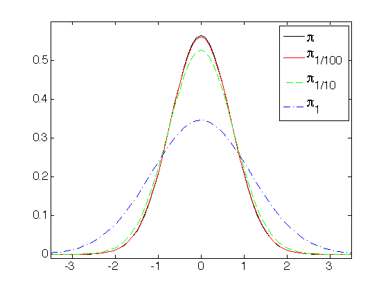
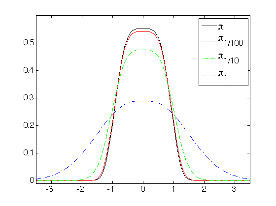
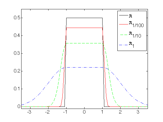
To illustrate these definitions, Fig. 1 depicts the Moreau approximations of four distributions that are log-concave: the Laplace distribution $\pi(x)\propto\exp{\left(-|x|\right)}$, the Gaussian distribution $\pi(x)\propto\exp{\left(-x^{2}\right)}$, the quartic or fourth-order polynomial distribution $\pi(x)\propto\exp{\left(-x^{4}\right)}$, and the uniform distribution $\pi(x)\propto\boldsymbol{1}(\boldsymbol{x})_{[-1,1]}$. We observe that the approximations are smooth, converge to $\pi$ as $\lambda$ decreases, and have the same maximisers as the true densities, as described by Properties 1, 2 and 4. We also observe that for densities with lighter-than-Gaussian tails the Moreau approximation mimics the true density around the mode but has Gaussian tails, as described by Property 6.

As mentioned previously, the methods proposed in this paper are useful for models that have proximity mappings which are easy to evaluate or to approximate numerically (see Section 3.2.3 for more details). This is the case for many statistical models used in high-dimensional data analysis, where statistical inference is often conducted using convex optimisation algorithms that also require computing proximity mappings (see Afonso et al. (2011); Becker et al. (2009); Recht et al. (2010); Chandrasekaran et al. (2012) for examples in image restoration, compressive sensing, low-rank matrix recovery and graphical model selection). For more details about the evaluation of these mappings, their properties, and lists of functions with known mappings please see Bauschke and Combettes (2011), Combettes and Pesquet (2011) and Parikh and Boyd (2014, Ch. 6). A library with MATLAB implementations of frequently used proximity mappings is available on \urlhttps://github.com/cvxgrp/proximal.

The sampling method presented in this paper is derived from the Langevin diffusion process and is related to other Langevin MCMC algorithms that we briefly recall below.

Suppose that $\pi$ is everywhere non-zero and differentiable so that $\nabla\log\pi$ is well defined. Then let $W$ be the $n$-dimensional Brownian motion and consider a Langevin diffusion process $\{Y(t):0\leq t\leq T\}$ on $\mathbb{R}^{n}$ that has $\pi$ as stationary distribution. Such process is defined as the solution to the stochastic differential equation

Under appropriate stability conditions, $Y(t)$ converges in distribution to $\pi$ and is therefore potentially interesting for simulating from $\pi$. Unfortunately, direct simulation from $Y(t)$ is only possible in very specific cases. A more general solution is to consider a discrete-time approximation of the Langevin diffusion process with step-size $\delta$. For computational reasons a forward Euler approximation is typically used, resulting in the so-called ULA

where the parameter $\delta$ controls the discrete-time increment as well as the variance of the Gaussian perturbation $Z^{(m)}$. Under certain conditions on $\pi$ and $\delta$, ULA produces a good approximation of $Y(t)$ and converges to an ergodic measure which is close to $\pi$. In MALA this approximation error is corrected by introducing a rejection step that guarantees convergence to the correct target density $\pi$ (Roberts and Tweedie, 1996).

It is well known that MALA can be a very efficient sampling method, particularly in high-dimensional problems. However, it is also known that for certain classes of target densities ULA is transient and as a result MALA is not geometrically ergodic (Roberts and Tweedie, 1996). Geometric ergodicity is important theoretically to guarantee the existence of a central limit theorem for the chains and practically because sub-geometric algorithms often fail to explore the parameter space properly. Another limitation of MALA and HMC methods is that they require $\pi\in\mathcal{C}^{1}$. This limits their applicability in many popular image processing and machine models that are not smooth.

In the following section we present a new MALA method that use proximity mappings and Moreau approximations to capture the log-concavity of the target density and construct chains with significantly better geometric convergence properties. We emphasise at this point that this is not the first work to consider modifications of MALA with better geometric convergence properties. For example, Roberts and Tweedie (1996) suggested using MALA with a truncated gradient to retain the efficiency of the Langevin proposal near the density’s mode and add robustness in the tails, though we have found this approach to be difficult to implement practically (this is illustrated in Section 3.2.4). Also, Casella et al. (2011) recently proposed three variations of MALA based on implicit discretisation schemes that are geometrically ergodic for one-dimensional distributions with super-exponential tails. For certain one-dimensional densities the methods presented in this paper are closely related to the partially implicit schemes of Casella et al. (2011). Manifold MALA (Girolami and Calderhead, 2011) is also geometrically ergodic for a wide range of tail behaviours if $\delta$ is sufficiently small (Łatuszyński, Roberts, Thiéry and Wolny, 2011).

In image deconvolution or deblurring problems, the goal is to recover an original image $\boldsymbol{x}\in\mathbb{R}^{n}$ from a blurred and noisy observed image $\boldsymbol{y}\in\mathbb{R}^{n}$ related to $\boldsymbol{x}$ by the linear observation model²² 2 note that bidimensional and tridimensional images can be represented as points in $\mathbb{R}^{n}$ via lexicographic ordering. $\boldsymbol{y}=H\boldsymbol{x}+\boldsymbol{w}$, where $H$ is a linear operator representing the blur point spread function and $\boldsymbol{w}$ is the sample of a zero-mean white Gaussian vector with covariance matrix $\sigma^{2}\boldsymbol{I}_{n}$ (Hansen et al., 2006). This inverse problem is usually ill-posed or ill-conditioned, i.e., either $H$ does not admit an inverse or it is nearly singular, thus yielding highly noise-sensitive solutions. Bayesian image deconvolution methods address this difficulty by exploiting prior knowledge about $\boldsymbol{x}$ in order to obtain more robust estimates. One of the most widely used image priors for deconvolution problems is the improper total-variation norm prior, $\pi(\boldsymbol{x})\propto\exp{\left(-\alpha\|\nabla_{d}\boldsymbol{x}\|_{1}\right)}$, where $\nabla_{d}$ denotes the discrete gradient operator that computes the vertical and horizontal differences between neighbour pixels. This prior encodes the fact that differences between neighbour image pixels are often very small and occasionally take large values (i.e., image gradients are nearly sparse). Based on this prior and on the linear observation model described above, the posterior distribution for $\boldsymbol{x}$ is given by

Image processing methods using (14) are almost exclusively based on maximum-a-posteriori (MAP) estimates of $\boldsymbol{x}$ that can be efficiency computed using proximal optimisation algorithms (Afonso et al., 2011). Here we consider the problem of computing credibility regions for $\boldsymbol{x}$, which we use to assess the confidence in the restored image. Precisely, we note that (14) is log-concave and use P-MALA to compute marginal $90\%$ credibility regions for each image pixel. There are several computational strategies for evaluating the proximity mapping of $g(\boldsymbol{x})=-\|\boldsymbol{y}-H\boldsymbol{x}\|^{2}/2\sigma^{2}-\alpha\|\nabla\boldsymbol{x}\|_{1}$. Here we take advantage of the fact that in high-dimensional scenarios $\delta$ is typically set to a small value and use the approximation (12) $\operatorname{prox}^{\delta/2}_{g}(\boldsymbol{x})\approx\operatorname{prox}^{\delta/2}_{g_{2}}\{\boldsymbol{x}+\delta\nabla g_{1}(\boldsymbol{x})/2\}$ with $g_{1}(\boldsymbol{x})=-\|\boldsymbol{y}-H\boldsymbol{x}\|^{2}/2\sigma^{2}$ and $g_{2}(\boldsymbol{x})=-\alpha\|\nabla\boldsymbol{x}\|_{1}$, and where we note that $\nabla g_{1}$ is Lipschitz continuous and that $\operatorname{prox}^{\delta/2}_{g_{2}}(\boldsymbol{x})$ can be efficiently computed using a parallel implementation of Chambolle (2004).

Figure 3 presents an experiment with the “cameraman” image, which is a standard image to assess deconvolution methods (Oliveira et al., 2009). Figures 3(a) and (b) show the original cameraman image ${\boldsymbol{x}}_{0}$ of size $128\times 128$ and a blurred and noisy observation $\boldsymbol{y}$, which we produced by convoluting ${\boldsymbol{x}}_{0}$ with a uniform blur of size $9\times 9$ and adding white Gaussian noise to achieve a blurred signal-to-noise ratio (BSNR) of $40$dB ($BRSN=10\log_{10}\{\textrm{var}(H{\boldsymbol{x}}_{0})/\sigma^{2}\}$). The MAP estimate of $\boldsymbol{x}$ obtained by maximising (14) is depicted in Figure 3(c). This estimate has been computed with the proximal optimisation algorithm of Afonso et al. (2011), and by using the technique of Oliveira et al. (2009) to determine the value of $\alpha$. By comparing Figures 3(a) and 3(c) we observe that the MAP estimate is very accurate and that it restored the sharp edges and fine details in the image. Finally, Figure 3(d) shows the magnitude of the marginal $90\%$ credibility regions for each pixels, as measured by the distance between the $95\%$ and $5\%$ quantile estimates. These estimates were computed from a $20\,000$-sample chain generated with P-MALA using a thinning factor of $1\,000$ to reduce the algorithm’s memory foot-print and $1$ million burn-in iterations. These credibility regions show that there is a background level of uncertainty of about $30$ grey-levels, which is approximately $10\%$ of the dynamic range of the image ($256$ grey-levels). More importantly, we observe that there is significantly more uncertainty concentrated at the contours and object boundaries in the image. This reveals that model (14) is able to accurately detect the presence of sharp edges in the image but with some uncertainty about their exact location. Therefore computing credibility regions could be particularly relevant in applications that use images to determine the location and the size of objects, or to compare the size of a same object appearing in two different images. For example, in oncological medical imaging, where deconvolution is increasingly used to improve the resolution of images that are subsequently used to assess the evolution of tumour boundaries over time and make treatment decisions.

Moreover, to asses the efficiency of P-MALA we repeated the experiment with a variation of MALA for partially non-differentiable target densities that uses only the gradient of the differentiable term of (14), i.e., $\nabla\log g_{1}(\boldsymbol{x})=H^{T}(\boldsymbol{y}-H\boldsymbol{x})/\sigma^{2}$ (this variation of MALA was recently used in Schreck et al. (2013) for a Bayesian variable selection problem with a Bernulli–Laplace prior that is also non-differentiable). Figure 4 compares the first $20$ lags of the sample autocorrelation function of the chains generated with P-MALA and MALA, computed using $\log\pi(\boldsymbol{x}|\boldsymbol{y})$ as scalar summary. We observe that the chain produced with P-MALA has significantly lower autocorrelation and therefore higher effective sample size³³ 3 Recall that $ESS=N\{1+2\sum_{k}\gamma(k)\}^{-1}$, where $N$ is the total samples and $\sum_{k}\gamma(k)$ is the sum of the $K$ monotone sample auto-correlations which we estimated with the initial monotone sequence estimator (Geyer, 1992) (ESS). P-MALA was almost twice as computationally expensive as MALA due to the overhead associated with evaluating the proximity mapping of $g_{2}$ (the total computational times were $49$ hours for P-MALA and $28$ hours for MALA). However, because P-MALA is exploring the parameter space significantly faster than MALA, its time-normalised ESS was $4.5$ times better than that of MALA ($50.8$ and $11.04$ samples per hour respectively), confirming the good performance of the proposed methodology. Preconditioning MALA with the (regularised) inverse Fisher information matrix $(H^{T}H+\epsilon\mathbb{I}_{n})^{-1}$ led to poor mixing, possibly because most of the correlation structure in the posterior distributions comes from the non-differentiable prior $\pi(\boldsymbol{x})\propto\exp{[-\alpha\|\nabla_{d}\boldsymbol{x}\|_{1}]}$ and is not captured by this metric.

In this experiment we use P-MALA to perform a graphical posterior predictive check of the widely used nuclear norm model for low-rank matrices (Fazel, 2002). Simulating samples from distributions involving the nuclear norm is challenging because matrices are often high-dimensional and because this norm is not continuously differentiable; thus making it difficult to use gradient-based MCMC methods such as MALA and HMC. For simplicity we present our analysis in the context of matrix denoising, however the approach can be easily applied to other low-rank matrix estimation problems such as matrix completion and decomposition (Chandrasekaran et al., 2011; Chandrasekaran et al., 2012; Candès and Plan, 2009; Candès and Tao, 2009; Candès et al., 2011).

Let $\boldsymbol{x}$ be an unknown low-rank matrix of size $n=n_{1}\times n_{2}$ (represented as a point in $\mathbb{R}^{n}$ by lexicographic ordering), and $\boldsymbol{y}=\boldsymbol{x}+\boldsymbol{w}$ a noisy observation contaminated by zero-mean white Gaussian noise with covariance matrix $\sigma^{2}\boldsymbol{I}_{n}$. For example, $\boldsymbol{x}$ can represent a low-rank covariance matrix in a model selection problem, the background component of a video signal in an object tracking problem, or a rank-limited image in a signal restoration or reconstruction problem (Chandrasekaran et al., 2012; Candès et al., 2011; Recht et al., 2010). In the low-rank matrix denoising problem, we seek to recover $\boldsymbol{x}$ from $\boldsymbol{y}$ under the prior knowledge that $\boldsymbol{x}$ has low rank; that is, that most of its singular values are zero. A convenient model for this type of problem is the nuclear norm prior $\pi(\boldsymbol{x})\propto\exp(-\alpha||\boldsymbol{x}||_{*})$, where $||\boldsymbol{x}||_{*}$ denotes the nuclear norm of $\boldsymbol{x}$ and is defined as the sum of its singular values (Fazel, 2002). The popularity of this prior stems from the fact that the nuclear norm is the best convex approximation of the rank function, and it leads to a posterior distribution that is log-concave and whose MAP estimate can be efficiently computed using proximal algorithms (Recht et al., 2010). The posterior distribution of $\boldsymbol{x}$ given $\boldsymbol{y}$ is

where $\sigma^{2}$ and $\alpha$ are fixed positive hyper-parameters. It is useful to think of (15) as an extension the Bayesian LASSO model (Park and Casella, 2008) to matrices with sparse singular values, in which the singular values of $\boldsymbol{x}$ are assigned exponential priors.

It is well documented that under certain conditions on the true rank and $\sigma^{2}$, the MAP estimate maximising (15) accurately recovers the true null and column spaces of $\boldsymbol{x}$ (Candès and Plan, 2009; Candès and Tao, 2009; Negahban and Wainwright, 2012; Rahul et al., 2010). This has led to the general consensus that the nuclear-norm prior is a useful model for low-rank matrix estimation problems and that the errors introduced by using the convex approximation to the rank function do not have a significant effect on the inferences. Here we adopt a Bayesian model checking viewpoint and assess the nuclear-norm model by comparing the observation $\boldsymbol{y}$ to replicas $\boldsymbol{y}^{rep}$ generated by drawing samples from the posterior predictive distribution $f(\boldsymbol{y}^{rep}|\boldsymbol{y})=\int_{\mathbb{R}^{n\times m}}f(\boldsymbol{y}^{rep}|\boldsymbol{x})\pi(\boldsymbol{x}|\boldsymbol{x})\textrm{d}\boldsymbol{x}$, as recommended by Gelman et al. (2013, Ch. 6). This technique for checking the fit of a model to data is based on the intuition that “If the model fits, then replicated data generated under the model should look similar to observed data. To put it another way, the observed data should look plausible under the posterior predictive distribution.” (Gelman et al., 2013, Ch. 6). In this paper we perform a graphical check and compare visually $\boldsymbol{y}$ and its replicas $\boldsymbol{y}^{rep}$. In specific applications one could also use $\boldsymbol{y}^{rep}$ to compute posterior predictive p-values that evaluate specific aspects of the model that are relevant to the application (Gelman et al., 2013, Ch. 6).

Figure 5 presents an experiment with MATLAB’s “checkerboard” image. Figure 5(a) shows the original checkerboard image $\boldsymbol{x}_{0}$ of size $n=64\times 64$ pixels and rank $2$. Figure 5(b) shows a noisy observation $\boldsymbol{y}$ produced by adding Gaussian noise with variance $\sigma^{2}=0.01$, leading to a signal-to-noise ratio (SNR) of $15$dB which is standard for image denoising problems ($SNR=10\log_{10}(||\boldsymbol{x}_{0}||^{2}/nm\sigma^{2})$). The MAP estimate obtained by maximising (15) is depicted in Figure 5(c). This estimate has been computed via singular value soft-thresholding, and by setting $\alpha=1.15/\sigma^{2}$ to minimise Stein’s unbiased risk estimator, which are standard procedures in low-rank matrix denoising (Candès et al., 2013). By comparing Figures 5(a) and 5(c) we observe that the MAP estimate is indeed very close the the original image $\boldsymbol{x}_{0}$, confirming that the nuclear norm prior is a good model for low-rank signals (the estimation mean-squared error is $6.45\times 10^{-4}$, which is $15$ times better than the original error of $0.01$). Note however that this prior is a simplistic model for $\boldsymbol{x}_{0}$ in the sense that it does not include many of its main features; e.g., that $\boldsymbol{x}_{0}$ is piecewise constant, periodic, highly symmetric, or that its pixel only take 3 values. Also, its representation of the singular values is approximate given that the true singular values are perfectly sparse rather than exponentially distributed. Therefore it is interesting to examine if the predictions of the model exhibit all the relevant features of $\boldsymbol{y}$, or if they highlight limitations of (15).

Figures 5(d)-(i) depict six random replicas of $\boldsymbol{y}$ drawn from the posterior predictive distribution $f(\boldsymbol{y}^{rep}|\boldsymbol{y})$ generated with P-MALA. We observe that the replicas are visually very similar to the original observation depicted in Figure 5(b) and exhibit all of the main structural features of the checkerboard pattern that we mentioned above (e.g., periodicity, symmetries, etc.) as well as a grey-level histogram that is very similar to that of $\boldsymbol{y}$. This suggests that the model is indeed capturing the main visual characteristics our data. The replicas for this experiment were generated by using P-MALA to simulate $N=20\,000$ samples $\{X^{(t)},t=1,\ldots,N\}$ distributed according to (15), and then sampling $Y^{rep(t)}|X^{(t)}\sim\mathcal{N}[X^{(t)},\boldsymbol{I}\sigma^{2}]$ (the pictures displayed in Figure 5(d)-(i) correspond to $t=7\,500,10\,000,12\,500,15\,000,17\,500$, and $20\,000$). To implement P-MALA for (15) we used the exact proximity mapping

where $SVT(\boldsymbol{x},\tau)$ denotes the singular value soft-thresholding operator on $\boldsymbol{x}$ with threshold $\tau$, that is evaluated by computing the singular value representation of $\boldsymbol{x}$ and replacing the singular values $\{s_{i}:i=1,\ldots,\min(n1,n2)\}$ with $\max{(s_{i}-\tau,0)}$. We used $2\,000$ burn-in iterations, a thinning factor of $100$ to reduce the algorithm’s memory foot-print, and tuned the value of $\delta$ to achieve an acceptance probability of approximately $50\%$.

To illustrate the good mixing properties of P-MALA for this $4\,096$-dimensional simulation problem, Figure 6 shows a $1\,000$-sample trace plot and an autocorrelation function plot of the chain $\{X^{(t)},t=1,\ldots,N\}$, where we have used $g[X^{(t)}]$ as scalar summary. The computing time, ESS and time-normalised ESS for this experiment are $19$ minutes, $7\,930$ samples and $7.05$ samples per second. For comparison, repeating this experiment with a random walk (RWMH) algorithm required $6.5$ minutes and produced a time-normalised ESS of $0.23$ samples per second, approximately $30$ times worse than P-MALA. Finally, note that MALA and HMC are not well defined for this model because $||\boldsymbol{x}||_{*}$ is not differentiable at points where $\boldsymbol{x}$ is rank deficient. From a practical standpoint one can still apply MALA to (15) because the probability of reaching a non-differentiable state is zero, however in our experience MALA does require $\pi\in\mathcal{C}^{1}$ to perform well. Repeating this experiment with MALA produced a time-normalised ESS of $0.08$ samples per second, $90$ times worse than P-MALA and $30$ times worse than RWHM (results computed by setting $\delta$ to achieve an acceptance rate of approximately $60\%$ and by computing the gradient of $||\boldsymbol{x}||_{*}$ via singular-value decomposition (Papadopoulo and Lourakis, 2000)).

References

- Afonso et al. (2011) Afonso, M., Bioucas-Dias, J. and Figueiredo, M. (2011), ‘An augmented Lagrangian approach to the constrained optimization formulation of imaging inverse problems’, IEEE. Trans. on Image Process. 20(3), 681–695.
- Agarwal et al. (2012) Agarwal, A., Negahban, S. and Wainwright, J. M. (2012), ‘Fast global convergence of gradient methods for high-dimensional statistical recovery’, Ann. Statist. 40(5), 2452–2482.
- Atchade (2006) Atchade, Y. (2006), ‘An adaptive version for the Metropolis adjusted Langevin algorithm with a truncated drift’, Method. Comput. in App. 8(2), 235–254.
- Bauschke and Combettes (2011) Bauschke, H. H. and Combettes, P. L. (2011), Convex Analysis and Monotone Operator Theory in Hilbert Spaces, Springer New York.
- Becker et al. (2009) Becker, S., Bobin, J. and Candès, E. J. (2009), ‘NESTA: a fast and accurate first-order method for sparse recovery’, SIAM J. on Imaging Sci. 4(1), 1–39.
- Candès et al. (2011) Candès, E. J., Li, X., Ma, Y. and Wright, J. (2011), ‘Robust principal component analysis?’, J. ACM 58(3).
- Candès and Plan (2009) Candès, E. J. and Plan, Y. (2009), ‘Matrix completion with noise’, Proc. IEEE 98(6), 925–936.
- Candès et al. (2013) Candès, E. J., Sing-Long, C. A. and Trzasko, J. D. (2013), ‘Unbiased risk estimates for singular value thresholding and spectral estimators’, IEEE Trans. on Signal Process. 61(19), 4643–4657.
- Candès and Tao (2009) Candès, E. J. and Tao, T. (2009), ‘The power of convex relaxation: Near-optimal matrix completion’, IEEE Trans. Inform. Theory 56(5), 2053–2080.
- Candès and Wakin (2008) Candès, E. J. and Wakin, M. B. (2008), ‘An introduction to compressive sampling’, IEEE Signal Process. Mag. 25(2), 21–30.
- Casella et al. (2011) Casella, B., Roberts, G. and Stramer, O. (2011), ‘Stability of partially implicit Langevin schemes and their MCMC variants’, Methodol. and Comput. Appl. 13(4), 835–854.
- Chaari et al. (2014) Chaari, L., Batatia, H., Chaux, C. and Tourneret, J.-Y. (2014), ‘Sparse signal and image recovery using a proximal Bayesian algorithm’, ArXiv e-prints .
- Chambolle (2004) Chambolle, A. (2004), ‘An algorithm for total variation minimization and applications’, J. Math. Imaging Vis. 20(1-2), 89–97.
- Chandrasekaran and Jordan (2013) Chandrasekaran, V. and Jordan, M. I. (2013), ‘Computational and statistical tradeoffs via convex relaxation’, PNAS 110(13), 1181–1190.
- Chandrasekaran et al. (2012) Chandrasekaran, V., Parrilo, P. A. and Willsky, A. S. (2012), ‘Latent variable graphical model selection via convex optimization’, Ann. Statist. 40(4), 1935–1967.
- Chandrasekaran et al. (2011) Chandrasekaran, V., Sanghavi, S., Parrilo, P. and Willsky, A. (2011), ‘Rank-sparsity incoherence for matrix decomposition’, SIAM J. OPTIMIZ 21(2), 572–596.
- Combettes and Pesquet (2011) Combettes, P. L. and Pesquet, J.-C. (2011), Proximal splitting methods in signal processing, in H. H. Bauschke, R. S. Burachik, P. L. Combettes, V. Elser, D. R. Luke and H. Wolkowicz, eds, ‘Fixed-Point Algorithms for Inverse Problems in Science and Engineering’, Springer New York, pp. 185–212.
- Combettes and Wajs (2005) Combettes, P. and Wajs, V. (2005), ‘Signal recovery by proximal forward-backward splitting’, Multiscale Model Sim. 4(4), 1168–1200.
- Fazel (2002) Fazel, M. (2002), Matrix rank minimization with applications, PhD thesis, Ph.D. thesis, Dept. Elec. Eng., Stanford Univ.
- Gelman et al. (2013) Gelman, A., Carlin, J. B., Stern, H. S., Dunson, D. B., Vehtari, A. and Rubin, D. B. (2013), Bayesian data analysis, 3rd ed., Chapman and Hall/CRC.
- Geyer (1992) Geyer, C. J. (1992), ‘Practical Markov chain Monte Carlo’, Statistic. Science 7(4), 473–483.
- Girolami and Calderhead (2011) Girolami, M. and Calderhead, B. (2011), ‘Riemann manifold Langevin and Hamiltonian Monte Carlo methods’, J. Roy. Stat. Soc. Ser. B 73(2), 123–214.
- Hansen et al. (2006) Hansen, P. C., Nagy, J. G. and O’Leary, D. P. (2006), Deblurring Images: Matrices, Spectra, and Filtering, SIAM, Philadelphia.
- Higham et al. (2003) Higham, D. J., Mao, X. and Stuart, A. M. (2003), ‘Strong convergence of Euler-type methods for nonlinear stochastic differential equations’, SIAM J. Numer. Anal. 40(3), 1041 – 1063.
- Komodakis and Pesquet (2014) Komodakis, N. and Pesquet, J.-C. (2014), ‘Playing with Duality: An Overview of Recent Primal-Dual Approaches for Solving Large-Scale Optimization Problems’, ArXiv e-prints . Łatuszyński et al.
- Łatuszyński, Roberts, Thiéry and Wolny (2011) Łatuszyński, K., Roberts, G. O., Thiéry, A. and Wolny, K. (2011), ‘Discussion of Riemann manifold Langevin and Hamiltonian Monte Carlo methods by Mark Girolami and Ben Calderhead’, J. Roy. Stat. Soc. Ser. B 73(2), 188–189.
- Marnissi et al. (2014) Marnissi, Y., Benazza-Benyahia, A., Chouzenoux, E. and Pesquet, J.-C. (2014), Majorize-Minimize adapted Metropolis-Hastings algorithm. Application to multichannel image recovery, in ‘22th European Signal Processing Conference’, (EUSIPCO 2014), Lisbon, Portugal.
- Martinet (1970) Martinet, B. (1970), ‘Regularisation d’inéquations variationelles par approximations successives’, Revue Fran. d’Automatique et Infomatique Rech. Opérationelle 4, 154–159.
- Mattingly et al. (2002) Mattingly, J., Stuart, A. and Higham, D. (2002), ‘Ergodicity for SDEs and approximations: locally Lipschitz vector fields and degenerate noise’, Stoch. Proc. Appl. 101(2), 185 – 232.
- Meyn and Tweedie (1993) Meyn, S. and Tweedie, R. (1993), Markov Chains and Stochastic Stability, Springer-Verlag, London.
- Moreau (1962) Moreau, J.-J. (1962), ‘Fonctions convexes duales et points proximaux dans un espace Hilbertien’, C. R. Acad. Sci. Paris Sér. A Math. 255, 2897–2899.
- Neal (2012) Neal, R. (2012), ‘MCMC using Hamiltonian dynamics’, ArXiv e-prints .
- Negahban and Wainwright (2012) Negahban, S. and Wainwright, M. J. (2012), ‘Restricted strong convexity and weighted matrix completion: Optimal bounds with noise’, J. Mach. Learn. Res. 13, 1665–1697.
- Oliveira et al. (2009) Oliveira, J., Bioucas-Dias, J. and Figueiredo, M. (2009), ‘Adaptive total variation image deblurring: A majorization-minimization approach’, Signal Process. 89(9), 1683–1693.
- Ottobre and Stuart (2014) Ottobre, M. and Stuart, A. M. (2014), ‘Diffusion limit for the random walk Metropolis algorithm out of stationarity’, ArXiv e-prints .
- Papadopoulo and Lourakis (2000) Papadopoulo, T. and Lourakis, M. I. A. (2000), Estimating the Jacobian of the singular value decomposition: Theory and applications, in ‘Proceedings of the 6th European Conference on Computer Vision-Part I’, ECCV ’00, pp. 554–570.
- Parikh and Boyd (2014) Parikh, N. and Boyd, S. (2014), ‘Proximal algorithms’, Foundations and Trends in Optimization 1(3), 123–231.
- Park and Casella (2008) Park, T. and Casella, G. (2008), ‘The Bayesian lasso’, J. Am. Statist. Assoc. 103(482), 681–686.
- Pereyra (2013) Pereyra, M. (2013), ‘Proximal Markov chain Monte Carlo algorithms’, ArXiv e-prints .
- Pesquet and Pustelnik (2012) Pesquet, J.-C. and Pustelnik, N. (2012), ‘A parallel inertial proximal optimization method’, Pac. J. Optim. 8(2), 273–305.
- Pillai et al. (2012) Pillai, N. S., Stuart, A. M. and Thiéry, A. H. (2012), ‘Optimal scaling and diffusion limits for the Langevin algorithm in high dimensions’, Ann. Appl. Probab. 22(6), 2320–2356.
- Rahul et al. (2010) Rahul, M., Trevor, H. and Robert, T. (2010), ‘Spectral regularization algorithms for learning large incomplete matrices’, J. Mach. Learn. Res. 11, 2287–2322.
- Recht et al. (2010) Recht, B., Fazel, M. and Parrilo, P. A. (2010), ‘Guaranteed minimum rank solutions to linear matrix equations via nuclear norm minimization’, SIAM Rev. 52(3), 471–501.
- Robert and Casella (2004) Robert, C. P. and Casella, G. (2004), Monte Carlo Statistical Methods, 2nd ed., Springer-Verlag, New York.
- Roberts and Tweedie (1996) Roberts, G. O. and Tweedie, R. L. (1996), ‘Exponential convergence of Langevin distributions and their discrete approximations’, Bernulli 2(4), 341–363.
- Roberts and Stramer (2002) Roberts, G. and Stramer, O. (2002), ‘Langevin diffusions and Metropolis-Hastings algorithms’, Methodol. Comput. Appl. Probab. 4, 337–357.
- Rockafellar (1976) Rockafellar, R. T. (1976), ‘Monotone operators and the proximal point algorithm’, SIAM J. Control Optim. 14, 877–898.
- Schreck et al. (2013) Schreck, A., Fort, G., Le Corff, S. and Moulines, E. (2013), ‘A shrinkage-thresholding Metropolis adjusted Langevin algorithm for Bayesian variable selection’, ArXiv e-prints .
- Stramer and Tweedie (1999a) Stramer, O. and Tweedie, R. L. (1999a), ‘Langevin-type models I: Diffusions with given stationary distributions and their discretizations’, Methodol. Comput. Appl. Probab. 1, 283–306.
- Stramer and Tweedie (1999b) Stramer, O. and Tweedie, R. L. (1999b), ‘Langevin-type models II: Self-targeting candidates for MCMC algorithms’, Methodol. Comput. Appl. Probab. 1, 307–328.
- Yuan and Minka (2002) Yuan, Q. and Minka, T. P. (2002), ‘Hessian-based Markov chain Monte Carlo Algorithms’, Unpublished manuscript .
- Zhang and Sutton (2011) Zhang, Y. and Sutton, C. (2011), ‘Quasi-Newton Markov chain Monte Carlo’, In Advances in Neural Information Processing Systems (NIPS) .