跳到论文正文
W Papers独立论文阅读器 arXiv:1306.0094 论文正文 计算阅读时间 · 0%
引用这篇论文根据当前论文元数据生成,正式投稿前建议核对。


License: arXiv.org perpetual non-exclusive license
arXiv:1306.0094v1 [cs.IT] 01 Jun 2013

Analysis of Mismatched Estimation Errors Using Gradients of Partition Functions∗Thanks: ∗This research was partially supported by The Israeli Science Foundation (ISF), grant no. 412/12.

Wasim Huleihel and Neri Merhav Affiliation: Department of Electrical Engineering Affiliation: Technion - Israel Institute of Technology Affiliation: Haifa 32000, ISRAEL Affiliation: E-mail: {wh@tx, merhav@ee}.technion.ac.il
Abstract

We consider the problem of signal estimation (denoising) from a statistical-mechanical perspective, in continuation to a recent work on the analysis of mean-square error (MSE) estimation using a direct relationship between optimum estimation and certain partition functions. The paper consists of essentially two parts. In the first part, using the aforementioned relationship, we derive single-letter expressions of the mismatched MSE of a codeword (from a randomly selected code), corrupted by a Gaussian vector channel. In the second part, we provide several examples to demonstrate phase transitions in the behavior of the MSE. These examples enable us to understand more deeply and to gather intuition regarding the roles of the real and the mismatched probability measures in creating these phase transitions.

Index Terms: 
Minimum mean-square error (MMSE), mismatched MSE, partition function, statistical-mechanics, conditional mean estimation, phase transitions, threshold effect.

I Introduction

The connections and the interplay between information theory, statistical physics and signal estimation have been known for several decades [1, 2, 3, 4], and they are still being studied from a variety of aspects, see, for example [5, 6, 7, 8, 9, 10, 11, 12, 13, 14, 15, 16, 17] and many references therein.

Recently, in [6], the well known I-MMSE relation [8], which relates the mutual information and the derivative of the minimum mean-square error (MMSE), was further explored using a statistical physics perspective. Specifically, in their analysis, the authors of [6] exploit the natural “mapping” between information theory problems and certain models of many-particle systems in statistical mechanics (see, e.g., [18, 19]). One of the main contributions in [6] is the demonstration of the usefulness of statistical-mechanical tools (in particular, utilizing the fact that the mutual information can be viewed as the partition function of a certain physical system) in assessing MMSE via the I-MMSE relation of [8]. More recently, Merhav [5] proposed a more flexible method, whose main idea is that, for the purpose of evaluating the covariance matrix of the MMSE estimator, one may use other information measures, which have the form of a partition function and hence can be analyzed using methods of statistical physics (see, e.g., [18, 19, 20, 21, 22, 23, 24, 25, 26] and many references therein). The main advantage of the proposed approach over the I-MMSE relations, is its full generality: Any joint probability function P⁡(𝒙,𝒚)P\left(\mbox{\boldmath$x$},\mbox{\boldmath$y$}\right), where 𝒙x and 𝒚y designate the channel input to be estimated and the channel output, respectively, can be handled (for example, the channel does not have to be additive or Gaussian). Moreover, using this approach, any mismatch, both in the source and the channel, can be considered.

This paper is a further development of [5] in the above described direction. Particularly, in [5, Section IV. A], the problem of mismatched estimation of a codeword, transmitted over an additive white Gaussian (AWGN) channel, was considered. It was shown that the mismatched MSE exhibits phase transitions at some rate thresholds, which depend upon the real and the mismatched parameters of the problem, and the behavior of the receiver. To wit, the mismatched MSE acts inherently differently for a pessimistic and optimistic receivers, where in the example considered in [5, Section IV. A] pessimism literally means that the estimator assumes that the channel is worse than it really is (in terms of signal-to-noise ratio (SNR)), and the vice versa for optimism. In this paper, we extend the above described model to a much more general one; the Gaussian vector channel, which has a plenty of applications in communications and signal processing. It is important to emphasize that compared to [5, 6], it will be seen that: (1) the mathematical analysis is much more complicated (consisting of some new concepts), and (2) the notions of pessimism and optimism described above, also play a significant role in this model, although their physical meanings in general are not obvious. Moreover, in contrast to previous work on mismatched estimation, in this paper, the interesting case of channel mismatch is explored, namely, the receiver has a wrong assumption on the channel. In order to demonstrate the usefulness of the theoretical results derived for the general model, we also provide a few examples associated with some specific channel transfer functions, and draw conclusions and insights regarding the threshold effects in the behavior of the partition function and the MSE.

As was mentioned earlier, we consider the Gaussian vector channel model

𝒀=𝑨𝑿+𝑵,\displaystyle\mbox{\boldmath$Y$}=\mbox{\boldmath$A$}\mbox{\boldmath$X$}+\mbox{\boldmath$N$}, (1)

where 𝑵∈ℝn\mbox{\boldmath$N$}\in\mathbb{R}^{n} is a Gaussian white noise vector and 𝑨A is a deterministic n×nn\times n matrix representing a linear transformation induced by a given linear system. The vector 𝑿∈ℝn\mbox{\boldmath$X$}\in\mathbb{R}^{n} is chosen uniformly at random from a codebook (which is itself selected at random as well). There are several motivations for codeword estimation. One example is that of a user that, in addition to its desired signal, receives also a relatively strong interference signal, which carries digital information intended to other users, and which comes from a codebook whose rate exceeds the capacity of this crosstalk channel between the interferer and our user, so that the user cannot fully decode this interference. Nevertheless, our user would like to estimate the interference as accurately as possible for the purpose of cancellation. Furthermore, we believe that the tools/concepts developed in this paper for handling matched and mismatched problems, can be used in other applications in signal processing and communication. Such examples are denoising (see for example, [27, 28, 29]), mismatched decoding (for example, [30]), blind deconvolution (for example, [31, 32]), and many other applications. Note that although the aforementioned examples are radically different (in terms of their basic models and systematization), they will all suffer from mismatch when estimating the input signals.

In the special case of matched estimation, it will be shown that the MMSE is asymptotically given by

limn→∞mmse​(𝑿∣𝒀)n={12​π∫02​πPx1+|𝐇⁡(ω)|2​Px​βdω,ifR>Rc0,ifR≤Rc\displaystyle\lim_{n\to\infty}\frac{\text{mmse}\left(\mbox{\boldmath$X$}\mid\mbox{\boldmath$Y$}\right)}{n}=\begin{cases}\frac{1}{2\pi}\int_{0}^{2\pi}\frac{P_{x}}{1+\left|{\bf{H}}\left(\omega\right)\right|^{2}P_{x}\beta}\mathrm{d}\omega,\ \ &\text{if}\ \ R>R_{c}\\ 0,\ \ &\text{if}\ \ R\leq R_{c}\\ \end{cases} (2)

where

Rc=△14​π​∫02​πln⁡(1+|𝐇⁡(ω)|2​Px​β)​𝑑ω,\displaystyle R_{c}\stackrel{{\scriptstyle\triangle}}{{=}}\frac{1}{4\pi}\int_{0}^{2\pi}\ln\left(1+\left|{\bf{H}}\left(\omega\right)\right|^{2}P_{x}\beta\right)\mathrm{d}\omega, (3)

in which mmse​(𝑿∣𝒀)\text{mmse}\left(\mbox{\boldmath$X$}\mid\mbox{\boldmath$Y$}\right) is the estimation error results from estimating 𝑿X based on 𝒀Y, using the MMSE estimator, 1/β1/\beta and PxP_{x} denote the noise variance and the transmitted power, respectively, and 𝐇⁡(ω){\bf{H}}\left(\omega\right) is the frequency response of the linear system 𝑨A. As can be seen from the above formula, for R<RcR<R_{c} the MMSE essentially vanishes since the correct codeword can be reliably decoded, whereas for R>RcR>R_{c}, the MMSE is simply the estimation error which results by the Wiener filter that would have been applied had the input been a zero-mean, i.i.d. Gaussian process, with variance 1/β1/\beta. Accordingly, it will be seen that for R>RcR>R_{c} the MMSE estimator is simply the Wiener filter. It is important to emphasize that while the above result may seem to be a natural generalization of the results in [5, 6] (where 𝑨A is taken to be identity matrix), the analysis (and results) of the mismatched case is by far more complicated and non-trivial. Indeed, it will be seen that in the mismatched case, the MSE is essentially separated into two cases, each exhibiting a completely different behavior. Further physical insights regarding the above result and other results will be presented later on.

The remaining part of this paper is organized as follows. In Section II, we first establish notation conventions. Then, the model considered is presented and the problem is formulated. In Section III, the main results are stated and discussed. In Section IV, we provide a few examples which illustrate the theoretical results. In Section V, we discuss the techniques and methodologies that are utilized in order to prove the main results, along with a brief background and summary on the basic relations between the conditional mean estimator, as well as its error covariance matrix and the aforementioned partition function, which were derived in [5]. In Section VI, the main results are proved. Finally, our conclusions appear in Section VII.

II Notation Conventions and Problem Formulation

II-A Notation Conventions

Throughout this paper, scalar random variables (RV’s) will be denoted by capital letters, their sample values will be denoted by the respective lower case letters and their alphabets will be denoted by the respective calligraphic letters. A similar convention will apply to random vectors and their sample values, which will be denoted with same symbols in the bold face font. Thus, for example, 𝑿X will denote a random vector (X1,…,Xn)\left(X_{1},\ldots,X_{n}\right) and 𝒙=(x1,…,xn)\mbox{\boldmath$x$}=\left(x_{1},\ldots,x_{n}\right) is a specific vector value in 𝒳n{\cal X}^{n}, the nn-th Cartesian power of 𝒳{\cal X}. The notations 𝒙ij\mbox{\boldmath$x$}_{i}^{j} and 𝑿ij\mbox{\boldmath$X$}_{i}^{j}, where ii and jj are integers and i≤ji\leq j, will designate segments (xi,…,xj)\left(x_{i},\ldots,x_{j}\right) and (Xi,…,Xj)\left(X_{i},\ldots,X_{j}\right), respectively. Probability functions will be denoted generically by the letter PP or P′P^{\prime}. In particular, P⁡(𝒙,𝒚)P\left(\mbox{\boldmath$x$},\mbox{\boldmath$y$}\right) is the joint probability mass function (in the discrete case) or the joint density (in the continuous case) of the desired channel input vector 𝒙x and the observed channel output vector 𝒚y. Accordingly, P⁡(𝒙)P\left(\mbox{\boldmath$x$}\right) will denote the marginal of 𝒙x, P⁡(𝒚∣𝒙)P\left(\mbox{\boldmath$y$}\mid\mbox{\boldmath$x$}\right) will denote the conditional probability or density of 𝒚y given 𝒙x, induced by the channel, and so on.

The expectation operator of a generic function f⁡(𝒙,𝒚)f\left(\mbox{\boldmath$x$},\mbox{\boldmath$y$}\right) with respect to (w.r.t.) the joint distribution of 𝑿X and 𝒀Y, P⁡(𝒙,𝒚),P\left(\mbox{\boldmath$x$},\mbox{\boldmath$y$}\right), will be denoted by 𝑬​{f⁡(𝑿,𝒀)}\mbox{\boldmath$E$}\left\{f\left(\mbox{\boldmath$X$},\mbox{\boldmath$Y$}\right)\right\}. Accordingly, 𝑬′​{f⁡(𝑿,𝒀)}\mbox{\boldmath$E$}^{\prime}\left\{f\left(\mbox{\boldmath$X$},\mbox{\boldmath$Y$}\right)\right\} means that the expectation is performed w.r.t. P′​(𝒙,𝒚)P^{\prime}\left(\mbox{\boldmath$x$},\mbox{\boldmath$y$}\right). The conditional expectation of the same function given that 𝒀=𝒚\mbox{\boldmath$Y$}=\mbox{\boldmath$y$}, denoted 𝑬​{f⁡(𝑿,𝒀)∣𝒀=𝒚}\mbox{\boldmath$E$}\left\{f\left(\mbox{\boldmath$X$},\mbox{\boldmath$Y$}\right)\mid\mbox{\boldmath$Y$}=\mbox{\boldmath$y$}\right\} and which is obviously identical to 𝑬​{f⁡(𝑿,𝒚)∣𝒀=𝒚}\mbox{\boldmath$E$}\left\{f\left(\mbox{\boldmath$X$},\mbox{\boldmath$y$}\right)\mid\mbox{\boldmath$Y$}=\mbox{\boldmath$y$}\right\}, is, of course, a function of 𝒚y. On substituting 𝒀Y in this function, this becomes a random variable which will be denoted by 𝑬​{f⁡(𝑿,𝒀)∣𝒀}\mbox{\boldmath$E$}\left\{f\left(\mbox{\boldmath$X$},\mbox{\boldmath$Y$}\right)\mid\mbox{\boldmath$Y$}\right\}. When using vectors and matrices in a linear-algebraic format, nn-dimensional vectors, like 𝒙x (and 𝑿X), will be understood as column vectors, the operators (⋅)T\left(\cdot\right)^{T} and (⋅)H\left(\cdot\right)^{H} will denote vector or matrix transposition and vector or matrix conjugate transposition, respectively, and so, 𝒙T\mbox{\boldmath$x$}^{T} would be a row vector. For two positive sequences {an}\left\{a_{n}\right\} and {bn}\left\{b_{n}\right\}, the notation an=⋅bna_{n}\stackrel{{\scriptstyle\cdot}}{{=}}b_{n} means equivalence in the exponential order, i.e., limn→∞1n​log⁡(an/bn)=0\lim_{n\to\infty}\frac{1}{n}\log\left(a_{n}/b_{n}\right)=0. For two sequences {an}\left\{a_{n}\right\} and {bn}\left\{b_{n}\right\}, the notations an∼bna_{n}\sim b_{n} and an≲bna_{n}\lesssim b_{n} mean limn→∞(an/bn)=1\lim_{n\to\infty}\left(a_{n}/b_{n}\right)=1 and limn→∞(an/bn)≤1\lim_{n\to\infty}\left(a_{n}/b_{n}\right)\leq 1, respectively. Finally, the indicator function of an event 𝒜{\cal A} will be denoted by 𝟙​{𝒜}{\mathds{1}}{\left\{{\cal A}\right\}}.

II-B Model and Problem Formulation

Let 𝒞={𝒙0,…,𝒙M−1}{\cal C}=\left\{\mbox{\boldmath$x$}_{0},\ldots,\mbox{\boldmath$x$}_{M-1}\right\} denote a codebook of size M=en​RM=e^{nR}, which is selected at random (and then revealed to the estimator) in the following manner: Each 𝒙i\mbox{\boldmath$x$}_{i} is drawn independently under the uniform distribution over the surface of the nn-dimensional hyperesphere, which is centered at the origin, and whose radius is n​Px\sqrt{nP_{x}}. Finally, let 𝑿X assume a uniform distribution over 𝒞{\cal C}. We consider the Gaussian vector channel model

𝒀=𝑨𝑿+𝑵,\displaystyle\mbox{\boldmath$Y$}=\mbox{\boldmath$A$}\mbox{\boldmath$X$}+\mbox{\boldmath$N$}, (4)

where 𝒀Y, 𝑿X and 𝑵N are random vectors in ℝn\mathbb{R}^{n}, designating the channel output vector, the transmitted codeword and the noise vector, respectively. It is assumed that the components of the noise vector, 𝑵N, are i.i.d., zero-mean, Gaussian random variables with variance 1/β1/\beta, where β\beta is a given positive constant designating the signal-to-noise ratio (SNR) (for Px=1P_{x}=1), or the inverse temperature in the statistical-mechanical jargon. We further assume that 𝑿X and 𝑵N are statistically independent. Finally, the channel matrix, 𝑨∈ℝn×n\mbox{\boldmath$A$}\in\mathbb{R}^{n\times n}, is assumed to be a given deterministic Toeplitz matrix, whose entries are given by the coefficients of the impulse response of a given linear system. Specifically, let {hk}\left\{h_{k}\right\} denote the generating sequence (or impulse response) of 𝑨A, so that 𝑨={ai,j}i,j={hi−j}i,j\mbox{\boldmath$A$}=\left\{a_{i,j}\right\}_{i,j}=\left\{h_{i-j}\right\}_{i,j}, and let 𝐇⁡(ω){\bf{H}}\left(\omega\right) designate the frequency response (Fourier transform) of {hk}\left\{h_{k}\right\}.

As was mentioned previously, we analyze the problem of mismatched codeword estimation which is formulated as follows: Consider a mismatched estimator which is the conditional mean of 𝑿X given 𝒀Y, based on an incorrect joint distribution P′​(𝒙,𝒚)P^{\prime}\left(\mbox{\boldmath$x$},\mbox{\boldmath$y$}\right), whereas the true joint distribution continues to be P⁡(𝒙,𝒚)P\left(\mbox{\boldmath$x$},\mbox{\boldmath$y$}\right). Accordingly, the mismatched MSE is defined as

mse​(𝑿∣𝒀)\displaystyle\text{mse}\left(\mbox{\boldmath$X$}\mid\mbox{\boldmath$Y$}\right) =△𝑬​‖𝑿−𝑬′​{𝑿∣𝒀}‖2\displaystyle\stackrel{{\scriptstyle\triangle}}{{=}}\mbox{\boldmath$E$}\left\|\mbox{\boldmath$X$}-\mbox{\boldmath$E$}^{\prime}\left\{\mbox{\boldmath$X$}\mid\mbox{\boldmath$Y$}\right\}\right\|^{2} (5)

where 𝑬′​{𝑿∣𝒀}\mbox{\boldmath$E$}^{\prime}\left\{\mbox{\boldmath$X$}\mid\mbox{\boldmath$Y$}\right\} is the conditional expectation w.r.t. the mismatched measure P′P^{\prime}. In this paper, the following mismatch mechanism is assumed: The input measure is matched, i.e., P​(𝒙)=P′​(𝒙)P\left(\mbox{\boldmath$x$}\right)=P^{\prime}\left(\mbox{\boldmath$x$}\right) (namely, the mismatched estimator knows the true code), both conditional measures (“channels”) P(⋅∣𝒙)P\left(\cdot\mid\mbox{\boldmath$x$}\right) and P′(⋅∣𝒙)P^{\prime}\left(\cdot\mid\mbox{\boldmath$x$}\right) are Gaussian, but are associated with different channel matrices. More precisely, while the true channel matrix (under PP) is 𝑨A, the assumed channel matrix (under P′P^{\prime}) is 𝑨′\mbox{\boldmath$A$}^{\prime}, another Toeplitz matrix, generated by the impulse response {hk′}\left\{h_{k}^{\prime}\right\}, whose frequency response is 𝐇′​(ω){\bf{H}}^{\prime}\left(\omega\right). It should be pointed out, however, that the analysis in this paper can be easily carried out also for the case of mismatch in the input distribution, or mismatch in the noise distribution, which has been already considered in [5]. Using the theoretical tools derived in [5], the mismatched MSE (and the MMSE as a special case) will be derived for the model described above.

A very important function, which will be pivotal to our derivation of both the mismatched estimator and the MSE, is the partition function, which is defined as follows.

Definition 1 (Partition Function)

Let 𝝀=(λ1,…,λn)T\mbox{\boldmath$\lambda$}=\left(\lambda_{1},\ldots,\lambda_{n}\right)^{T} be a column vector of nn real-valued parameters. The partition function w.r.t. the joint distribution P⁡(𝒙,𝒚)P\left(\mbox{\boldmath$x$},\mbox{\boldmath$y$}\right), denoted by Z⁡(𝒚,𝝀)Z\left(\mbox{\boldmath$y$},\mbox{\boldmath$\lambda$}\right), is defined as

Z⁡(𝒚,𝝀)\displaystyle Z\left(\mbox{\boldmath$y$},\mbox{\boldmath$\lambda$}\right) =△∑𝒙∈𝒳nexp⁡{𝝀T​𝒙}​P​(𝒙,𝒚).\displaystyle\stackrel{{\scriptstyle\triangle}}{{=}}\sum_{\mbox{\boldmath$x$}\in{\cal X}^{n}}\exp\left\{\mbox{\boldmath$\lambda$}^{T}\mbox{\boldmath$x$}\right\}P\left(\mbox{\boldmath$x$},\mbox{\boldmath$y$}\right). (6)

In the above definition, it is assumed that the sum (or integral, in the continuous case) converges uniformly at least in some neighborhood of 𝝀=𝟎\mbox{\boldmath$\lambda$}=\mbox{\boldmath$0$} 11 1 In case that this assumption does not hold, one can instead, parametrize each component λi\lambda_{i} of 𝝀\lambda as a purely imaginary number λi=j​ωi\lambda_{i}=j\omega_{i} where i=−1i=\sqrt{-1}, similarly to the definition of the characteristics function.. Accordingly, under the above described model, the mismatched partition function is given by

Z′​(𝒚,𝝀)\displaystyle Z^{\prime}\left(\mbox{\boldmath$y$},\mbox{\boldmath$\lambda$}\right) =△∑𝒙∈𝒞exp⁡{𝝀T​𝒙}​P′​(𝒙,𝒚)\displaystyle\stackrel{{\scriptstyle\triangle}}{{=}}\sum_{\mbox{\boldmath$x$}\in{\cal C}}\exp\left\{\mbox{\boldmath$\lambda$}^{T}\mbox{\boldmath$x$}\right\}P^{\prime}\left(\mbox{\boldmath$x$},\mbox{\boldmath$y$}\right) (7)
=(2π/β)−n/2∑𝒙∈𝒞e−n​Rexp[−β‖𝒚−𝑨′𝒙‖2/2+𝝀T𝒙].\displaystyle=\left(2\pi/\beta\right)^{-n/2}\sum_{\mbox{\boldmath$x$}\in{\cal C}}e^{-nR}\exp\left[-\beta\left\|\mbox{\boldmath$y$}-\mbox{\boldmath$A$}^{\prime}\mbox{\boldmath$x$}\right\|^{2}/2+\mbox{\boldmath$\lambda$}^{T}\mbox{\boldmath$x$}\right]. (8)
Remark 1

In the above definition, the role of 𝝀\lambda will be understood later on. In a nutshell, the idea [5] is that the gradient of ln⁡Z′​(𝒚,𝝀)\ln Z^{\prime}\left(\mbox{\boldmath$y$},\mbox{\boldmath$\lambda$}\right) w.r.t. 𝝀\lambda, computed at 𝝀=𝟎\mbox{\boldmath$\lambda$}=\mbox{\boldmath$0$}, simply gives the mismatched MSE estimator, 𝑬′​{𝑿∣𝒚}\mbox{\boldmath$E$}^{\prime}\left\{\mbox{\boldmath$X$}\mid\mbox{\boldmath$y$}\right\}, and the expectation of the Hessian of ln⁡Z′​(𝒚,𝝀)\ln Z^{\prime}\left(\mbox{\boldmath$y$},\mbox{\boldmath$\lambda$}\right) w.r.t. 𝝀\lambda, computed at 𝝀=𝟎\mbox{\boldmath$\lambda$}=\mbox{\boldmath$0$}, gives the MSE. Nevertheless, in the next section, where we present the main results, the dependency of the different quantities in 𝝀\lambda will not be apparent, as they will already be computed at 𝝀=𝟎\mbox{\boldmath$\lambda$}=\mbox{\boldmath$0$}.

III Main Results and Discussion

In this section, our main results are presented and discussed. The proofs of these results are provided in Section VI. The asymptotic MMSE, which is obtained as a special case of the mismatched case (P=P′P=P^{\prime}), is given in the following theorem.

Theorem 1 (Asymptotic MMSE)

Consider the model defined in Subsection II-B, and assume that the sequence {hk}k\left\{h_{k}\right\}_{k} is square summable. Then, the asymptotic MMSE is given by

limn→∞mmse​(𝑿∣𝒀)n={12​π∫02​πPx1+|𝐇⁡(ω)|2​Px​βdω,R>Rc0,R≤Rc\displaystyle\lim_{n\to\infty}\frac{\text{mmse}\left(\mbox{\boldmath$X$}\mid\mbox{\boldmath$Y$}\right)}{n}=\begin{cases}\frac{1}{2\pi}\int_{0}^{2\pi}\frac{P_{x}}{1+\left|{\bf{H}}\left(\omega\right)\right|^{2}P_{x}\beta}\mathrm{d}\omega,\ \ &\ \ R>R_{c}\\ 0,\ \ &\ \ R\leq R_{c}\\ \end{cases} (9)

where

Rc=△14​π​∫02​πln⁡(1+|𝐇⁡(ω)|2​Px​β)​𝑑ω.\displaystyle R_{c}\stackrel{{\scriptstyle\triangle}}{{=}}\frac{1}{4\pi}\int_{0}^{2\pi}\ln\left(1+\left|{\bf{H}}\left(\omega\right)\right|^{2}P_{x}\beta\right)\mathrm{d}\omega. (10)

From the above result, it can be seen that for R>RcR>R_{c} the MMSE is simply the estimation error which results by the Wiener filter that would have been applied had the input been a zero-mean, i.i.d. Gaussian process, with variance 1/β1/\beta. Accordingly, it is also shown in Section VI that the MMSE estimator is exactly the Wiener filter.

In the next theorem, we present the mismatched MSE. In contrast to the MMSE, unfortunately, the MSE does not lend itself to a simple closed-form expression. As will be seen in Section VI, this complexity stems from the complicated dependence of the partition function on 𝝀\lambda. Nevertheless, despite of the following non-trivial expressions, it should be emphasized that the obtained MSE expression has a single-letter formula, and thus, practically, it can be easily calculated at least numerically. Let us define the following auxiliary variables

Pa​(ω)=△\displaystyle P_{a}\left(\omega\right)\stackrel{{\scriptstyle\triangle}}{{=}} |𝐇′​(ω)|2​β​(2+Px​β​|𝐇⁡(ω)|2)+γ0(|𝐇′​(ω)|2​β+γ0)2\displaystyle\frac{\left|{\bf{H}}^{\prime}\left(\omega\right)\right|^{2}\beta\left(2+P_{x}\beta\left|{\bf{H}}\left(\omega\right)\right|^{2}\right)+\gamma_{0}}{\left(\left|{\bf{H}}^{\prime}\left(\omega\right)\right|^{2}\beta+\gamma_{0}\right)^{2}} (11)

where γ0\gamma_{0} is chosen such that ∫02​πPa​(ω)​𝑑ω=2​π​Px\int_{0}^{2\pi}P_{a}\left(\omega\right)\mathrm{d}\omega=2\pi P_{x}. Next define

𝐁⁡(ω)=△(|𝐇′​(ω)|2+γ0)−2​(|𝐇′​(ω)|2​β​(2+Px​β​|𝐇⁡(ω)|2)+γ0)(|𝐇′​(ω)|2+γ0)3\displaystyle{\bf{B}}\left(\omega\right)\stackrel{{\scriptstyle\triangle}}{{=}}\frac{\left(\left|{\bf{H}}^{\prime}\left(\omega\right)\right|^{2}+\gamma_{0}\right)-2\left(\left|{\bf{H}}^{\prime}\left(\omega\right)\right|^{2}\beta\left(2+P_{x}\beta\left|{\bf{H}}\left(\omega\right)\right|^{2}\right)+\gamma_{0}\right)}{\left(\left|{\bf{H}}^{\prime}\left(\omega\right)\right|^{2}+\gamma_{0}\right)^{3}} (12)
𝐂⁡(ω)=△2​β2​|𝐇′​(ω)|2​(|𝐇⁡(ω)|2+1β)​𝐁​(ω)1+4​β2​|𝐇′​(ω)|2​Pa​(ω)​(|𝐇⁡(ω)|2+1β)\displaystyle{\bf{C}}\left(\omega\right)\stackrel{{\scriptstyle\triangle}}{{=}}\frac{2\beta^{2}\left|{\bf{H}}^{\prime}\left(\omega\right)\right|^{2}\left(\left|{\bf{H}}\left(\omega\right)\right|^{2}+\frac{1}{\beta}\right){\bf{B}}\left(\omega\right)}{\sqrt{1+4\beta^{2}\left|{\bf{H}}^{\prime}\left(\omega\right)\right|^{2}P_{a}\left(\omega\right)\left(\left|{\bf{H}}\left(\omega\right)\right|^{2}+\frac{1}{\beta}\right)}} (13)
ϑ=△2+∫02​π[PxPx​γ0+Px​|𝐇′​(ω)|2​β−𝐂⁡(ω)]​𝑑ω∫02​π𝐁⁡(ω)​𝑑ω,\displaystyle\vartheta\stackrel{{\scriptstyle\triangle}}{{=}}2+\frac{\int_{0}^{2\pi}\left[\frac{P_{x}}{P_{x}\gamma_{0}+P_{x}\left|{\bf{H}}^{\prime}\left(\omega\right)\right|^{2}\beta}-{\bf{C}}\left(\omega\right)\right]\mathrm{d}\omega}{\int_{0}^{2\pi}{\bf{B}}\left(\omega\right)\mathrm{d}\omega}, (14)

and

𝚵1​(ω)=△−β​𝐇′⁣∗​(ω)(|𝐇′​(ω)|2+γ0)2​[ϑ−2​(|𝐇′​(ω)|2+γ0)2​Pa​(ω)+2​β2​|𝐇′​(ω)|2​(|𝐇⁡(ω)|2+1β)1+4​β2​|𝐇′​(ω)|2​Pa​(ω)​(|𝐇⁡(ω)|2+1β)].\displaystyle\mbox{\boldmath$\Xi$}_{1}\left(\omega\right)\stackrel{{\scriptstyle\triangle}}{{=}}-\frac{\beta{\bf{H}}^{\prime*}\left(\omega\right)}{\left(\left|{\bf{H}}^{\prime}\left(\omega\right)\right|^{2}+\gamma_{0}\right)^{2}}\left[\vartheta-\frac{2\left(\left|{\bf{H}}^{\prime}\left(\omega\right)\right|^{2}+\gamma_{0}\right)^{2}P_{a}\left(\omega\right)+2\beta^{2}\left|{\bf{H}}^{\prime}\left(\omega\right)\right|^{2}\left(\left|{\bf{H}}\left(\omega\right)\right|^{2}+\frac{1}{\beta}\right)}{\sqrt{1+4\beta^{2}\left|{\bf{H}}^{\prime}\left(\omega\right)\right|^{2}P_{a}\left(\omega\right)\left(\left|{\bf{H}}\left(\omega\right)\right|^{2}+\frac{1}{\beta}\right)}}\right]. (15)

Let ϵs,0\epsilon_{s,0}, α1,0\alpha_{1,0} and α2,0\alpha_{2,0} be the solution of the following set of three simultaneous equations:

R+14​π​∫02​πln⁡(2​ϵs,0Px​|𝐇′​(ω)|2​α2,0+2​Px​α1,0​ϵs,0)​𝑑ω=0\displaystyle R+\frac{1}{4\pi}\int_{0}^{2\pi}\ln\left(\frac{2\epsilon_{s,0}}{P_{x}\left|{\bf{H}}^{\prime}\left(\omega\right)\right|^{2}\alpha_{2,0}+2P_{x}\alpha_{1,0}\epsilon_{s,0}}\right)\mathrm{d}\omega=0 (16)
12​π​∫02​π4​α1,0​ϵ0,s2+|𝐇′​(ω)|2​α2,0​[(|𝐇⁡(ω)|2​Px+1β)​α2,0+2​ϵs,0](|𝐇′​(ω)|2​α2,0+2​α1,0​ϵs,0)2​𝑑ω=Px\displaystyle\frac{1}{2\pi}\int_{0}^{2\pi}\frac{4\alpha_{1,0}\epsilon_{0,s}^{2}+\left|{\bf{H}}^{\prime}\left(\omega\right)\right|^{2}\alpha_{2,0}\left[\left(\left|{\bf{H}}\left(\omega\right)\right|^{2}P_{x}+\frac{1}{\beta}\right)\alpha_{2,0}+2\epsilon_{s,0}\right]}{\left(\left|{\bf{H}}^{\prime}\left(\omega\right)\right|^{2}\alpha_{2,0}+2\alpha_{1,0}\epsilon_{s,0}\right)^{2}}\mathrm{d}\omega=P_{x} (17)
12​π​∫02​π4​α1,02​ϵs,02​(1+Px​β​|𝐇⁡(ω)|2)+4​|𝐇′​(ω)|2​α1,0​ϵs,02​β+2​|𝐇′​(ω)|4​α2,0​ϵs,0​β2​β​ϵs,0​(|𝐇′​(ω)|2​α2,0+2​α1,0​ϵs,0)2​𝑑ω=1.\displaystyle\frac{1}{2\pi}\int_{0}^{2\pi}\frac{4\alpha_{1,0}^{2}\epsilon_{s,0}^{2}\left(1+P_{x}\beta\left|{\bf{H}}\left(\omega\right)\right|^{2}\right)+4\left|{\bf{H}}^{\prime}\left(\omega\right)\right|^{2}\alpha_{1,0}\epsilon_{s,0}^{2}\beta+2\left|{\bf{H}}^{\prime}\left(\omega\right)\right|^{4}\alpha_{2,0}\epsilon_{s,0}\beta}{2\beta\epsilon_{s,0}\left(\left|{\bf{H}}^{\prime}\left(\omega\right)\right|^{2}\alpha_{2,0}+2\alpha_{1,0}\epsilon_{s,0}\right)^{2}}\mathrm{d}\omega=1. (18)

Then, we define

𝐊⁡(ω)=△2​β​ϵs,0​(|𝐇′​(ω)|2​α2,0+2​α1,0​ϵs,0)2\displaystyle{\bf{K}}\left(\omega\right)\stackrel{{\scriptstyle\triangle}}{{=}}2\beta\epsilon_{s,0}\left(\left|{\bf{H}}^{\prime}\left(\omega\right)\right|^{2}\alpha_{2,0}+2\alpha_{1,0}\epsilon_{s,0}\right)^{2} (19)
𝐓⁡(ω)=△4​α1,02​ϵs,02​(1+Px​β​|𝐇⁡(ω)|2)+4​β​|𝐇′​(ω)|2​α1,0​ϵs,02+2​|𝐇′​(ω)|4​α2,0​β​ϵs,0\displaystyle{\bf{T}}\left(\omega\right)\stackrel{{\scriptstyle\triangle}}{{=}}4\alpha_{1,0}^{2}\epsilon_{s,0}^{2}\left(1+P_{x}\beta\left|{\bf{H}}\left(\omega\right)\right|^{2}\right)+4\beta\left|{\bf{H}}^{\prime}\left(\omega\right)\right|^{2}\alpha_{1,0}\epsilon_{s,0}^{2}+2\left|{\bf{H}}^{\prime}\left(\omega\right)\right|^{4}\alpha_{2,0}\beta\epsilon_{s,0} (20)
𝐃⁡(ω)=△|𝐇′​(ω)|2​α2,0+2​α1,0​ϵs,0\displaystyle{\bf{D}}\left(\omega\right)\stackrel{{\scriptstyle\triangle}}{{=}}\left|{\bf{H}}^{\prime}\left(\omega\right)\right|^{2}\alpha_{2,0}+2\alpha_{1,0}\epsilon_{s,0} (21)
𝐑⁡(ω)=△4​α1,0​ϵs,02+|𝐇′​(ω)|2​α2,0​[α2,0​(|𝐇⁡(ω)|2​Px+2​ϵs,0)]\displaystyle{\bf{R}}\left(\omega\right)\stackrel{{\scriptstyle\triangle}}{{=}}4\alpha_{1,0}\epsilon_{s,0}^{2}+\left|{\bf{H}}^{\prime}\left(\omega\right)\right|^{2}\alpha_{2,0}\left[\alpha_{2,0}\left(\left|{\bf{H}}\left(\omega\right)\right|^{2}P_{x}+2\epsilon_{s,0}\right)\right] (22)
𝐐⁡(ω)=△ϵs,0​(Px​|𝐇′​(ω)|2​α2,0+2​Px​α1,0​ϵs,0)\displaystyle{\bf{Q}}\left(\omega\right)\stackrel{{\scriptstyle\triangle}}{{=}}\epsilon_{s,0}\left(P_{x}\left|{\bf{H}}^{\prime}\left(\omega\right)\right|^{2}\alpha_{2,0}+2P_{x}\alpha_{1,0}\epsilon_{s,0}\right) (23)
V=△12​π​∫02​πPx​|𝐇′​(ω)|2​α2,0ϵs,0​(Px​|𝐇′​(ω)|2​α2,0+2​Px​α1,0​ϵs,0)​𝑑ω\displaystyle V\stackrel{{\scriptstyle\triangle}}{{=}}\frac{1}{2\pi}\int_{0}^{2\pi}\frac{P_{x}\left|{\bf{H}}^{\prime}\left(\omega\right)\right|^{2}\alpha_{2,0}}{\epsilon_{s,0}\left(P_{x}\left|{\bf{H}}^{\prime}\left(\omega\right)\right|^{2}\alpha_{2,0}+2P_{x}\alpha_{1,0}\epsilon_{s,0}\right)}\mathrm{d}\omega (24)
F=△1V​12​π​∫02​πPx​|𝐇′​(ω)|2​r2+2​Px​ϵs,0​r1Px​|𝐇′​(ω)|2​α2,0+2​Px​α1,0​ϵs,0​𝑑ω\displaystyle F\stackrel{{\scriptstyle\triangle}}{{=}}\frac{1}{V}\frac{1}{2\pi}\int_{0}^{2\pi}\frac{P_{x}\left|{\bf{H}}^{\prime}\left(\omega\right)\right|^{2}r_{2}+2P_{x}\epsilon_{s,0}r_{1}}{P_{x}\left|{\bf{H}}^{\prime}\left(\omega\right)\right|^{2}\alpha_{2,0}+2P_{x}\alpha_{1,0}\epsilon_{s,0}}\mathrm{d}\omega (25)
γ1=△12​π∫02​π[8​α1,0​ϵs,02​(1+Px​β​|𝐇⁡(ω)|2)+4​β​|𝐇′​(ω)|2​ϵs,02𝐊⁡(ω)\displaystyle\gamma_{1}\stackrel{{\scriptstyle\triangle}}{{=}}\frac{1}{2\pi}\int_{0}^{2\pi}\left[\frac{8\alpha_{1,0}\epsilon_{s,0}^{2}\left(1+P_{x}\beta\left|{\bf{H}}\left(\omega\right)\right|^{2}\right)+4\beta\left|{\bf{H}}^{\prime}\left(\omega\right)\right|^{2}\epsilon_{s,0}^{2}}{{\bf{K}}\left(\omega\right)}\right.
−8​𝐓​(ω)​β​ϵs,02​(|𝐇′​(ω)|2​α2,0+2​α1,0​ϵs,0)𝐊2​(ω)]dω\displaystyle\ \ \ \ \ \ \ \ \ \ \ \ \ \ \ \ \ \ \left.-\frac{8{\bf{T}}\left(\omega\right)\beta\epsilon_{s,0}^{2}\left(\left|{\bf{H}}^{\prime}\left(\omega\right)\right|^{2}\alpha_{2,0}+2\alpha_{1,0}\epsilon_{s,0}\right)}{{\bf{K}}^{2}\left(\omega\right)}\right]\mathrm{d}\omega (26)
γ2=△12​π​∫02​π2​𝐊​(ω)​β​ϵs,0​|𝐇′​(ω)|4−4​𝐓​(ω)​β​ϵs,0​(|𝐇′​(ω)|2​α2,0+2​α1,0​ϵs,0)​|𝐇′​(ω)|2𝐊2​(ω)​𝑑ω\displaystyle\gamma_{2}\stackrel{{\scriptstyle\triangle}}{{=}}\frac{1}{2\pi}\int_{0}^{2\pi}\frac{2{\bf{K}}\left(\omega\right)\beta\epsilon_{s,0}\left|{\bf{H}}^{\prime}\left(\omega\right)\right|^{4}-4{\bf{T}}\left(\omega\right)\beta\epsilon_{s,0}\left(\left|{\bf{H}}^{\prime}\left(\omega\right)\right|^{2}\alpha_{2,0}+2\alpha_{1,0}\epsilon_{s,0}\right)\left|{\bf{H}}^{\prime}\left(\omega\right)\right|^{2}}{{\bf{K}}^{2}\left(\omega\right)}\mathrm{d}\omega (27)
γ3=△12​π∫02​π[8​α1,02​ϵs,0​(1+Px​β​|𝐇⁡(ω)|2)+8​β​ϵs,0​|𝐇′​(ω)|2​α1,0+2​β​α2,0​|𝐇′​(ω)|4𝐊⁡(ω)\displaystyle\gamma_{3}\stackrel{{\scriptstyle\triangle}}{{=}}\frac{1}{2\pi}\int_{0}^{2\pi}\left[\frac{8\alpha_{1,0}^{2}\epsilon_{s,0}\left(1+P_{x}\beta\left|{\bf{H}}\left(\omega\right)\right|^{2}\right)+8\beta\epsilon_{s,0}\left|{\bf{H}}^{\prime}\left(\omega\right)\right|^{2}\alpha_{1,0}+2\beta\alpha_{2,0}\left|{\bf{H}}^{\prime}\left(\omega\right)\right|^{4}}{{\bf{K}}\left(\omega\right)}\right.
−𝐓⁡(ω)​[2​β​(|𝐇′​(ω)|2​α2,0+2​α1,0​ϵs,0)2+8​β​ϵs,0​α1,0​(|𝐇′​(ω)|2​α2,0+2​α1,0​ϵs,0)]𝐊2​(ω)]dω\displaystyle\left.-\frac{{\bf{T}}\left(\omega\right)\left[2\beta\left(\left|{\bf{H}}^{\prime}\left(\omega\right)\right|^{2}\alpha_{2,0}+2\alpha_{1,0}\epsilon_{s,0}\right)^{2}+8\beta\epsilon_{s,0}\alpha_{1,0}\left(\left|{\bf{H}}^{\prime}\left(\omega\right)\right|^{2}\alpha_{2,0}+2\alpha_{1,0}\epsilon_{s,0}\right)\right]}{{\bf{K}}^{2}\left(\omega\right)}\right]\mathrm{d}\omega (28)
Υ⁡(ω)=△−4​β​α1,0​ϵs,0​α2,0−β​α2,02​|𝐇′​(ω)|2𝐊2​(ω)\displaystyle\Upsilon\left(\omega\right)\stackrel{{\scriptstyle\triangle}}{{=}}\frac{-4\beta\alpha_{1,0}\epsilon_{s,0}\alpha_{2,0}-\beta\alpha_{2,0}^{2}\left|{\bf{H}}^{\prime}\left(\omega\right)\right|^{2}}{{\bf{K}}^{2}\left(\omega\right)} (29)
η1=△12​π​∫02​π4​𝐃​(ω)​ϵs,02−4​𝐑​(ω)​ϵs,0𝐃3​(ω)​𝑑ω\displaystyle\eta_{1}\stackrel{{\scriptstyle\triangle}}{{=}}\frac{1}{2\pi}\int_{0}^{2\pi}\frac{4{\bf{D}}\left(\omega\right)\epsilon_{s,0}^{2}-4{\bf{R}}\left(\omega\right)\epsilon_{s,0}}{{\bf{D}}^{3}\left(\omega\right)}\mathrm{d}\omega (30)
η2=△12​π∫02​π[|𝐇′​(ω)|2​[(|𝐇⁡(ω)|2​Px+1β)​α2,0+2​ϵs,0]𝐃2​(ω)\displaystyle\eta_{2}\stackrel{{\scriptstyle\triangle}}{{=}}\frac{1}{2\pi}\int_{0}^{2\pi}\left[\frac{\left|{\bf{H}}^{\prime}\left(\omega\right)\right|^{2}\left[\left(\left|{\bf{H}}\left(\omega\right)\right|^{2}P_{x}+\frac{1}{\beta}\right)\alpha_{2,0}+2\epsilon_{s,0}\right]}{{\bf{D}}^{2}\left(\omega\right)}\right.
+|𝐇′​(ω)|2​α2,0​(|𝐇⁡(ω)|2​Px+1β)​𝐃​(ω)−2​𝐑​(ω)​|𝐇′​(ω)|2𝐃3​(ω)dω]\displaystyle\left.\ \ \ \ \ \ \ \ \ \ \ \ \ +\frac{\left|{\bf{H}}^{\prime}\left(\omega\right)\right|^{2}\alpha_{2,0}\left(\left|{\bf{H}}\left(\omega\right)\right|^{2}P_{x}+\frac{1}{\beta}\right){\bf{D}}\left(\omega\right)-2{\bf{R}}\left(\omega\right)\left|{\bf{H}}^{\prime}\left(\omega\right)\right|^{2}}{{\bf{D}}^{3}\left(\omega\right)}\mathrm{d}\omega\right] (31)
η3=△12​π​∫02​π8​𝐃​(ω)​α1,0​ϵs,0+2​𝐃​(ω)​|𝐇′​(ω)|2​α2,0−4​𝐑​(ω)​α1,0𝐃3​(ω)​𝑑ω\displaystyle\eta_{3}\stackrel{{\scriptstyle\triangle}}{{=}}\frac{1}{2\pi}\int_{0}^{2\pi}\frac{8{\bf{D}}\left(\omega\right)\alpha_{1,0}\epsilon_{s,0}+2{\bf{D}}\left(\omega\right)\left|{\bf{H}}^{\prime}\left(\omega\right)\right|^{2}\alpha_{2,0}-4{\bf{R}}\left(\omega\right)\alpha_{1,0}}{{\bf{D}}^{3}\left(\omega\right)}\mathrm{d}\omega (32)
Λ⁡(ω)=△α2,02𝐃2​(ω)\displaystyle\Lambda\left(\omega\right)\stackrel{{\scriptstyle\triangle}}{{=}}\frac{\alpha_{2,0}^{2}}{{\bf{D}}^{2}\left(\omega\right)} (33)
r1=η2​γ3−γ2​η3γ2​η1−η2​γ1\displaystyle r_{1}=\frac{\eta_{2}\gamma_{3}-\gamma_{2}\eta_{3}}{\gamma_{2}\eta_{1}-\eta_{2}\gamma_{1}} (34)
r2=η1​γ3−γ1​η3γ1​η2−η1​γ2\displaystyle r_{2}=\frac{\eta_{1}\gamma_{3}-\gamma_{1}\eta_{3}}{\gamma_{1}\eta_{2}-\eta_{1}\gamma_{2}} (35)
𝐉1​(ω)=η2​Υ​(ω)−γ2​Λ​(ω)γ2​η1−η2​γ1\displaystyle{\bf{J}}_{1}\left(\omega\right)=\frac{\eta_{2}\Upsilon\left(\omega\right)-\gamma_{2}\Lambda\left(\omega\right)}{\gamma_{2}\eta_{1}-\eta_{2}\gamma_{1}} (36)
𝐉2​(ω)=η1​Υ​(ω)−γ1​Λ​(ω)γ1​η2−η1​γ2\displaystyle{\bf{J}}_{2}\left(\omega\right)=\frac{\eta_{1}\Upsilon\left(\omega\right)-\gamma_{1}\Lambda\left(\omega\right)}{\gamma_{1}\eta_{2}-\eta_{1}\gamma_{2}} (37)
𝐉⁡(ω)=△12​π​𝐉1​(ω)​∫02​π2​ϵs,02​Px𝐐⁡(ω)​𝑑ω+𝐉2​(ω)​∫02​π2​ϵs,0​Px​|𝐇′​(ω)|2𝐐⁡(ω)​𝑑ωV⁡(1−F)\displaystyle{\bf{J}}\left(\omega\right)\stackrel{{\scriptstyle\triangle}}{{=}}\frac{1}{2\pi}\frac{{\bf{J}}_{1}\left(\omega\right)\int_{0}^{2\pi}\frac{2\epsilon_{s,0}^{2}P_{x}}{{\bf{Q}}\left(\omega\right)}\mathrm{d}\omega+{\bf{J}}_{2}\left(\omega\right)\int_{0}^{2\pi}\frac{2\epsilon_{s,0}P_{x}\left|{\bf{H}}^{\prime}\left(\omega\right)\right|^{2}}{{\bf{Q}}\left(\omega\right)}\mathrm{d}\omega}{V\left(1-F\right)} (38)
𝚵2​(ω)=△−2​𝐉​(ω)​𝐇′⁣∗​(ω).\displaystyle\mbox{\boldmath$\Xi$}_{2}\left(\omega\right)\stackrel{{\scriptstyle\triangle}}{{=}}-2{\bf{J}}\left(\omega\right){\bf{H}}^{\prime*}\left(\omega\right). (39)

Finally, let

Eg=△Px−Re⁡(1π​∫02​π𝚵2​(ω)∗​𝐇∗​(ω)​Px​𝑑ω)+12​π​∫02​π|𝚵2​(ω)|2​(|𝐇⁡(ω)|2​Px+1β)​𝑑ω,\displaystyle E_{g}\stackrel{{\scriptstyle\triangle}}{{=}}P_{x}-\re\left(\frac{1}{\pi}\int_{0}^{2\pi}\mbox{\boldmath$\Xi$}_{2}\left(\omega\right)^{*}{\bf{H}}^{*}\left(\omega\right)P_{x}\mathrm{d}\omega\right)+\frac{1}{2\pi}\int_{0}^{2\pi}\left|\mbox{\boldmath$\Xi$}_{2}\left(\omega\right)\right|^{2}\left(\left|{\bf{H}}\left(\omega\right)\right|^{2}P_{x}+\frac{1}{\beta}\right)\mathrm{d}\omega, (40)

and

Ep=△Px−Re⁡(1π​∫02​π𝚵1​(ω)∗​𝐇∗​(ω)​Px​𝑑ω)+12​π​∫02​π|𝚵1​(ω)|2​(|𝐇⁡(ω)|2​Px+1β)​𝑑ω,\displaystyle E_{p}\stackrel{{\scriptstyle\triangle}}{{=}}P_{x}-\re\left(\frac{1}{\pi}\int_{0}^{2\pi}\mbox{\boldmath$\Xi$}_{1}\left(\omega\right)^{*}{\bf{H}}^{*}\left(\omega\right)P_{x}\mathrm{d}\omega\right)+\frac{1}{2\pi}\int_{0}^{2\pi}\left|\mbox{\boldmath$\Xi$}_{1}\left(\omega\right)\right|^{2}\left(\left|{\bf{H}}\left(\omega\right)\right|^{2}P_{x}+\frac{1}{\beta}\right)\mathrm{d}\omega, (41)

and we define the following critical rates

Re=△\displaystyle R_{e}\stackrel{{\scriptstyle\triangle}}{{=}} 14​π​∫02​πln⁡(Px​γ0+Px​β​|𝐇′​(ω)|2)​𝑑ω\displaystyle\frac{1}{4\pi}\int_{0}^{2\pi}\ln\left(P_{x}\gamma_{0}+P_{x}\beta\left|{\bf{H}}^{\prime}\left(\omega\right)\right|^{2}\right)\mathrm{d}\omega (42)
Rd=△\displaystyle R_{d}\stackrel{{\scriptstyle\triangle}}{{=}} 12+β​Px​12​π​∫02​πRe⁡(𝐇′⁣∗​(ω)​𝐇​(ω))​𝑑ω\displaystyle\frac{1}{2}+\beta P_{x}\frac{1}{2\pi}\int_{0}^{2\pi}\re\left({\bf{H}}^{\prime*}\left(\omega\right){\bf{H}}\left(\omega\right)\right)\mathrm{d}\omega
+14​π∫02​π|𝐇′(ω)|2β(|𝐇′​(ω)|2​β​(2+β​|𝐇⁡(ω)|2​Px)+γ0(|𝐇′​(ω)|2​β+γ0)2−Px)\displaystyle+\frac{1}{4\pi}\int_{0}^{2\pi}\left|{\bf{H}}^{\prime}\left(\omega\right)\right|^{2}\beta\left(\frac{\left|{\bf{H}}^{\prime}\left(\omega\right)\right|^{2}\beta\left(2+\beta\left|{\bf{H}}\left(\omega\right)\right|^{2}P_{x}\right)+\gamma_{0}}{\left(\left|{\bf{H}}^{\prime}\left(\omega\right)\right|^{2}\beta+\gamma_{0}\right)^{2}}-P_{x}\right)
−14​π∫02​π|𝐇′​(ω)|2​β​(3+2​Px​β​|𝐇⁡(ω)|2)+γ0(|𝐇′​(ω)|2​β+γ0)\displaystyle-\frac{1}{4\pi}\int_{0}^{2\pi}\frac{\left|{\bf{H}}^{\prime}\left(\omega\right)\right|^{2}\beta\left(3+2P_{x}\beta\left|{\bf{H}}\left(\omega\right)\right|^{2}\right)+\gamma_{0}}{\left(\left|{\bf{H}}^{\prime}\left(\omega\right)\right|^{2}\beta+\gamma_{0}\right)} (43)
Rc=△\displaystyle R_{c}\stackrel{{\scriptstyle\triangle}}{{=}} Re+Rd\displaystyle R_{e}+R_{d} (44)
Rg=△\displaystyle R_{g}\stackrel{{\scriptstyle\triangle}}{{=}} −14​π∫02​πln(2​ϵ~Px​|𝐇′​(ω)|2​α~2+2​Px​α~1​ϵ~)dω\displaystyle-\frac{1}{4\pi}\int_{0}^{2\pi}\ln\left(\frac{2\tilde{\epsilon}}{P_{x}\left|{\bf{H}}^{\prime}\left(\omega\right)\right|^{2}\tilde{\alpha}_{2}+2P_{x}\tilde{\alpha}_{1}\tilde{\epsilon}}\right)\mathrm{d}\omega (45)

where α~1\tilde{\alpha}_{1} and α~2\tilde{\alpha}_{2} solve the set of two simultaneous equations

12​π​∫02​π4​α~1​ϵ~2+|𝐇′​(ω)|2​α~2​[(|𝐇⁡(ω)|2​Px+1β)​α~2+2​ϵ~](|𝐇′​(ω)|2​α~2+2​α~1​ϵ~)2​𝑑ω=Px\displaystyle\frac{1}{2\pi}\int_{0}^{2\pi}\frac{4\tilde{\alpha}_{1}\tilde{\epsilon}^{2}+\left|{\bf{H}}^{\prime}\left(\omega\right)\right|^{2}\tilde{\alpha}_{2}\left[\left(\left|{\bf{H}}\left(\omega\right)\right|^{2}P_{x}+\frac{1}{\beta}\right)\tilde{\alpha}_{2}+2\tilde{\epsilon}\right]}{\left(\left|{\bf{H}}^{\prime}\left(\omega\right)\right|^{2}\tilde{\alpha}_{2}+2\tilde{\alpha}_{1}\tilde{\epsilon}\right)^{2}}\mathrm{d}\omega=P_{x} (46)
12​π​∫02​π4​α~12​ϵ~2​(1+Px​β​|𝐇⁡(ω)|2)+4​|𝐇′​(ω)|2​α~1​ϵ~2​β+2​|𝐇′​(ω)|4​α~2​ϵ~​β2​β​ϵ~​(|𝐇′​(ω)|2​α~2+2​α~1​ϵ~)2​𝑑ω=1.\displaystyle\frac{1}{2\pi}\int_{0}^{2\pi}\frac{4\tilde{\alpha}_{1}^{2}\tilde{\epsilon}^{2}\left(1+P_{x}\beta\left|{\bf{H}}\left(\omega\right)\right|^{2}\right)+4\left|{\bf{H}}^{\prime}\left(\omega\right)\right|^{2}\tilde{\alpha}_{1}\tilde{\epsilon}^{2}\beta+2\left|{\bf{H}}^{\prime}\left(\omega\right)\right|^{4}\tilde{\alpha}_{2}\tilde{\epsilon}\beta}{2\beta\tilde{\epsilon}\left(\left|{\bf{H}}^{\prime}\left(\omega\right)\right|^{2}\tilde{\alpha}_{2}+2\tilde{\alpha}_{1}\tilde{\epsilon}\right)^{2}}\mathrm{d}\omega=1. (47)

and

ϵ~=12​β+Px4​π​∫02​π|𝐇′​(ω)−𝐇⁡(ω)|2​𝑑ω.\displaystyle\tilde{\epsilon}=\frac{1}{2\beta}+\frac{P_{x}}{4\pi}\int_{0}^{2\pi}\left|{\bf{H}}^{\prime}\left(\omega\right)-{\bf{H}}\left(\omega\right)\right|^{2}\mathrm{d}\omega. (48)

We are now in a position to state our main theorem.

Theorem 2 (Mismatched MSE)

Consider the model defined in Subsection II-B, and assume that the sequence {hk}k\left\{h_{k}\right\}_{k} is square summable. The (asymptotic) mismatched MSE is given as follows:
a) For Rd≥0R_{d}\geq 0

limn→∞mse​(𝑿∣𝒀)n={0,R≤RcEp,R>Rc.\displaystyle\lim_{n\to\infty}\frac{\text{mse}\left(\mbox{\boldmath$X$}\mid\mbox{\boldmath$Y$}\right)}{n}=\begin{cases}0,\ \ &\ \ R\leq R_{c}\\ E_{p},\ \ &\ \ R>R_{c}\end{cases}. (49)

b) For Rd<0R_{d}<0

limn→∞mse​(𝑿∣𝒀)n={0,R≤RgEg,Rg<R≤ReEp,R>Re.\displaystyle\lim_{n\to\infty}\frac{\text{mse}\left(\mbox{\boldmath$X$}\mid\mbox{\boldmath$Y$}\right)}{n}=\begin{cases}0,\ \ &\ \ R\leq R_{g}\\ E_{g},\ \ &\ \ R_{g}<R\leq R_{e}\\ E_{p},\ \ &\ \ R>R_{e}\end{cases}. (50)

In the jargon of statistical mechanics of spin arrays (see for example [33, Ch. 6]), the ranges of rates R≤RcR\leq R_{c} for Rd≥0R_{d}\geq 0, R≤RgR\leq R_{g} for Rd<0R_{d}<0, and R≤RcR\leq R_{c} in the matched case, correspond to the ordered phase (or ferromagnetic phase) in which the partition function is dominated by the correct codeword (and hence so is the posterior). Accordingly, in this range the MSE asymptotically vanishes, which literally means reliable communication. The intermediate range, Rg<R≤ReR_{g}<R\leq R_{e}, which appears only in the mismatched case and only for Rd<0R_{d}<0, is analogous to the glassy phase (or “frozen” phase), in which the partition function is dominated by a sub-exponential number of wrong codewords. Intuitively, in this range, we may have the illusion that there is relatively little uncertainty about the transmitted codeword, but this is wrong due to the mismatch (as the main support of the mismatched posterior belongs to incorrect codewords). The remaining range corresponds to the paramagnetic phase, in which the partition function is dominated by an exponential number of wrong codewords. In Section IV, we will link between each one of the two cases Rd≥0R_{d}\geq 0 and Rd<0R_{d}<0, to “pessimistic” and “optimistic” behaviors of the receiver, which were already mentioned in the Introduction.

It is tempting to think that there should not be a range of rates for which the MSE (MMSE) vanishes, as we deal with an estimation problem rather than a decoding problem. Nonetheless, since codewords are being estimated, and there are a finite number of them, for low enough rates (up to some critical rate) the posterior is dominated by the correct codeword, and thus asymptotically, the estimation can be regarded as a maximum a posteriori probability (MAP) estimation, and so the MSE vanishes. In the same breath, note that this is not the case if mismatch in the input distribution is considered. For example, if the receiver’s assumption on the transmitted energy is wrong, then no matter how low the rate is, there will always be an inherent error which stems from the fallacious averaging over a hypersphere with wrong radius (wrong codebook). Precisely, in this case, the estimated codeword will differ from the real one by an inevitable scaling of Px′/Px\sqrt{P_{x}^{\prime}/P_{x}}, where Px′P_{x}^{\prime} is the mismatched power.

Finally, it is important to emphasize that the mismatched MSE estimator and the MMSE estimator can also be obtained as a byproduct of the analysis. However, since they will add only little further insights into the problem, we do not present them here. The interested reader can find their explicit expressions in Section VI.

Remark 2

Although we have assumed that the transmitted codeword has a flat spectrum, the analysis can readily be extended to any input spectral density Sx​(ω)S_{x}\left(\omega\right). In Section VI, we discuss the technical issues that should be considered in order to modify the analysis to hold for this generalization. As a concrete simple example, in the case of MMSE estimation, one obtains

limn→∞mmse​(𝑿∣𝒀)n={12​π∫02​πSx​(ω)1+|𝐇⁡(ω)|2​Sx​(ω)​βdω,R>Rc0,R≤Rc\displaystyle\lim_{n\to\infty}\frac{\text{mmse}\left(\mbox{\boldmath$X$}\mid\mbox{\boldmath$Y$}\right)}{n}=\begin{cases}\frac{1}{2\pi}\int_{0}^{2\pi}\frac{S_{x}\left(\omega\right)}{1+\left|{\bf{H}}\left(\omega\right)\right|^{2}S_{x}\left(\omega\right)\beta}\mathrm{d}\omega,\ \ &\ \ R>R_{c}\\ 0,\ \ &\ \ R\leq R_{c}\\ \end{cases} (51)

where

Rc=△14​π​∫02​πln⁡(1+|𝐇⁡(ω)|2​Sx​(ω)​β)​𝑑ω.\displaystyle R_{c}\stackrel{{\scriptstyle\triangle}}{{=}}\frac{1}{4\pi}\int_{0}^{2\pi}\ln\left(1+\left|{\bf{H}}\left(\omega\right)\right|^{2}S_{x}\left(\omega\right)\beta\right)\mathrm{d}\omega. (52)

Nevertheless, our assumption on flat input spectrum is reasonable when there is uncertainty at the encoder concerning the frequency response of the channel, as there are no “preferred” frequencies. Finally, note that as an application of the above issue, one may wish to consider the minimization of the MMSE w.r.t. the input spectral density.

IV Examples

In this section, we provide a few examples in order to illustrate the theoretical results presented in the previous section. In particular, we present and explore the phase diagrams and the MSE’s as functions of the rate and some parameters of the mismatched channel. The main goal in these examples is further understanding of the role of the true and the mismatched probability measures in creating phase transitions.

Example 1

We start with a simple example where both 𝐇⁡(ω){\bf{H}}\left(\omega\right) and 𝐇′​(ω){\bf{H}}^{\prime}\left(\omega\right) are low-pass filters (LPFs) that differ in their cutoff frequencies and gains

𝐇⁡(ω)={1,|ω|≤π20,else,\displaystyle{\bf{H}}\left(\omega\right)=\begin{cases}1,\ &\left|\omega\right|\leq\frac{\pi}{2}\\ 0,\ &\text{else}\end{cases}, (53)

and

𝐇′​(ω)={χ,|ω|≤ωc0,else\displaystyle{\bf{H}}^{\prime}\left(\omega\right)=\begin{cases}\chi,\ &\left|\omega\right|\leq\omega_{c}\\ 0,\ &\text{else}\end{cases} (54)

for some χ>0\chi>0 and 0≤ωc≤π0\leq\omega_{c}\leq\pi. In the numerical calculations, we chose β=Px=1\beta=P_{x}=1. Figures 1 and 2 show, respectively, the phase diagrams and the MSE’s as functions of RR and ωc\omega_{c}, for various values of the gain χ\chi. The first obvious observation is that the maximum range of rates for which the ferromagnetic phase dominates the partition function occurs at ωc=π/2\omega_{c}=\pi/2 for each gain, as expected. Next, consider the case of χ=1\chi=1, which means that the gain is matched. In this case, it is observed that for ωc≤π/2\omega_{c}\leq\pi/2, there are two phases: the ferromagnetic phase and the paramagnetic phase, and hence, based on Theorem 2, Rd≥0R_{d}\geq 0. On the other hand, for ωc>π/2\omega_{c}>\pi/2, the glassy phase begins to play a role, and thus Rd<0R_{d}<0. Intuitively speaking, the case of ωc≤π/2\omega_{c}\leq\pi/2 corresponds to a pessimistic assumption of the receiver - lower bandwidth which translates to lower effective SNR, while ωc>π/2\omega_{c}>\pi/2 corresponds to an optimistic assumption - higher effective SNR. These behaviors are consistent with the results obtained in [5], where the case of mismatch in the noise variance was considered (while assuming that 𝑨=𝑨′\mbox{\boldmath$A$}=\mbox{\boldmath$A$}^{\prime} is the identity matrix).

In [5], Rd>0R_{d}>0 simply translates to β>β′\beta>\beta^{\prime} (the mismatched noise variance is larger than the actual one), namely, the estimator is pessimistic, while in the case of the reversed inequality it is overly optimistic. Accordingly, in the pessimistic case, the partition function exhibits a single phase transition, but at the price of a lower critical rate (compared to the matched case), which means that the range of rates for which reliable communication is possible is smaller. In the optimistic case, however, there is no loss in the critical rate, but there is a price of an additional phase transition. Now, for χ≠1\chi\neq 1, the notions of pessimism and optimism are not a priori obvious. For example, it can be seen that for χ<1\chi<1, and for a large enough cutoff frequency ωc\omega_{c}, the mismatched estimator can be regarded as an optimistic one. Also, for χ>1\chi>1, apparently, the “price” of being too optimistic in the gain results in a dominant range of the glassy phase. Finally, note that the fact that the range of rates for which the ferromagnetic region dominates the partition function (namely, vanishing MSE) is decreasing with the excess of the optimism (e.g., for χ=1\chi=1 and increasing of the cutoff frequency) is reasonable22 2 In [5], in contrast to our case, for β<β′\beta<\beta^{\prime} (Rd<0R_{d}<0), the critical rate ReR_{e} is fixed for any mismatched noise variance value, namely, it is independent of the optimistic behavior of the receiver.. Indeed, the uncertainty in the frequency domain, causes the receiver to assume that the codewords are distributed in some subspace of the nn-dimensional hypersphere. The size of this subspace is, of course, increasing as the receiver’s assumption is more optimistic. Accordingly, the probability of error also increases, and thus the threshold rate for reliable communication decreases.

Refer to caption

Fig. 1: Example 1: Phase diagram in the plane of RR vs. ωc\omega_{c} with various gain values. The arrows are directed towards the boundaries of the various phase transitions.

Refer to caption

Fig. 2: Example 1: Mismatched MSE as a function of RR and ωc\omega_{c} with various gain values.
Example 2

Let 𝐇⁡(ω){\bf{H}}\left(\omega\right) be a multiband filter given by

𝐇⁡(ω)={1,|ω±3​π8|≤π8​or​|ω±7​π8|≤π80,else,\displaystyle{\bf{H}}\left(\omega\right)=\begin{cases}1,\ &\left|\omega\pm\frac{3\pi}{8}\right|\leq\frac{\pi}{8}\;\text{or}\;\left|\omega\pm\frac{7\pi}{8}\right|\leq\frac{\pi}{8}\\ 0,\ &\text{else}\end{cases}, (55)

and let the mismatched filter be given by a band-pass filter

𝐇′​(ω)={1,ωL≤|ω|≤ωR0,else,\displaystyle{\bf{H}}^{\prime}\left(\omega\right)=\begin{cases}1,\ &\omega_{L}\leq\left|\omega\right|\leq\omega_{R}\\ 0,\ &\text{else}\end{cases}, (56)

with constant bandwidth, ωR−ωL=π/8\omega_{R}-\omega_{L}=\pi/8, i.e., smaller than the real one. In the numerical calculations, we again chose β=Px=1\beta=P_{x}=1. Figures 3 and 4 show, respectively, the phase diagram and the MSE as functions of RR and ωL\omega_{L}. First, observe that for ωR<π/4\omega_{R}<\pi/4, which means that 𝐇′​(ω){\bf{H}}^{\prime}\left(\omega\right) and 𝐇⁡(ω){\bf{H}}\left(\omega\right) are equal to one over non intersecting frequency ranges, there is no ferromagnetic phase, as expected. Accordingly, for ωR>π/4\omega_{R}>\pi/4, the ferromagnetic phase begins to play a role, and it can be seen that for π/4+π/8<ωR<π/2\pi/4+\pi/8<\omega_{R}<\pi/2, which means maximal intersection between the two filters, the range of rates for which the ferromagnetic phase dominates the partition function is maximal. Since the matched filter has two bands, obviously, the same behavior appears also in the second band. Thus, in this example, we actually obtain two disjoint glassy (and ferromagnetic) regions, which correspond to the two bands of the matched filter. Also, as shown in Fig. 4, in the ranges where no ferromagnetic phase exists, the MSE within the paramagnetic phase is larger than the MSE within the regions where ferromagnetic phase does exists, as one would expect.

Remark 3

Example 2 actually demonstrates that there can be arbitrarily many phase transitions. Generally speaking, for a matched multiband filter with NN disjoint bands, and a mismatched bandpass filter (with small enough bandwidth), there are NN disjoint glassy and ferromagnetic phases.

Refer to caption

Fig. 3: Example 2: Phase diagram in the plane of RR vs. ωL\omega_{L}.

Refer to caption

Fig. 4: Example 2: Mismatched MSE as a function of RR and ωL\omega_{L}.
Example 3

In this example, we consider more realistic filters. Let 𝐇⁡(z){\bf{H}}\left(z\right) denote a Type-II FIR filter given by (in the 𝒵\mathcal{Z} domain)

𝐇⁡(z)=(1−ej​0.8​π​z−1)2​(1−e−j​0.8​π​z−1)2,\displaystyle{\bf{H}}\left(z\right)=\left(1-e^{j0.8\pi}z^{-1}\right)^{2}\left(1-e^{-j0.8\pi}z^{-1}\right)^{2}, (57)

and let the mismatched filter be given is

𝐇′​(z)=(1−z0​z−1)​(1−z0∗​z−1)​(1−ej​0.8​π​z−1)​(1−e−j​0.8​π​z−1)\displaystyle{\bf{H}}^{\prime}\left(z\right)=\left(1-z_{0}z^{-1}\right)\left(1-z_{0}^{*}z^{-1}\right)\left(1-e^{j0.8\pi}z^{-1}\right)\left(1-e^{-j0.8\pi}z^{-1}\right) (58)

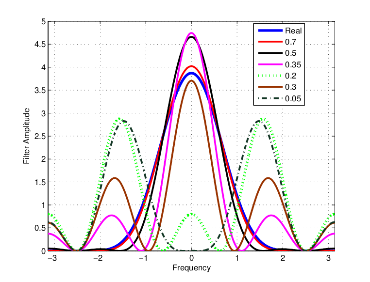
where z0z_{0} is a mismatched zero. In the numerical calculations, we chose again β=Px=1\beta=P_{x}=1. Fig. 5 shows the amplitude response of the real and the mismatched filters for various angular frequencies defined as ϕ=△arg⁡(z0)\phi\stackrel{{\scriptstyle\triangle}}{{=}}\arg\left(z_{0}\right). Figures 6 and 7 show, respectively, the phase diagram and the MSE as functions of RR and ϕ\phi. In this example, the roles of the differences between the true and mismatched filters, are emphasized. Starting with the obvious, observe that the maximal range of rates for which the ferromagnetic region dominates the partition function occurs at ϕ=0.8​π\phi=0.8\pi, as expected. Less trivially, for angular frequencies within the range [0.2​π,0.25​π]\left[0.2\pi,0.25\pi\right], the ferromagnetic region is negligible. Looking at Fig. 5, it can be seen that within this range of angular frequencies, the true and the mismatched filters are “almost orthogonal” in the L2L_{2} sense, namely, their inner product is almost zero. Accordingly, using the methods in Section VI, it can be easily shown that for orthogonal filters we have that Rg=0R_{g}=0, namely, no ferromagnetic region exists (note that in this example, RgR_{g} is never equal to zero since the filters are never orthogonal). Finally, for angular frequencies within the range [0,0.2​π]\left[0,0.2\pi\right], the ferromagnetic region returns to play a role. Indeed, Fig. 5 shows that, within this range, the matched and the mismatched filters “share” more similarities (in the sense of larger inner product).
Refer to caption

Fig. 5: Example 3: Amplitude of the real filter and mismatch filters for several phases.

Refer to caption

Fig. 6: Example 3: Phase diagram in the plane of RR vs. ϕ\phi.

Refer to caption

Fig. 7: Example 3: Mismatched MSE as a function of RR and ϕ\phi.
Example 4

Let 𝐇⁡(z){\bf{H}}\left(z\right) be given by

𝐇⁡(z)\displaystyle{\bf{H}}\left(z\right) =z−2​cos⁡(0.8​π)+z−1\displaystyle=z-2\cos\left(0.8\pi\right)+z^{-1}
=z⋅(1−ej​0.8​π​z−1)​(1−e−j​0.8​π​z−1)\displaystyle=z\cdot\left(1-e^{j0.8\pi}z^{-1}\right)\left(1-e^{-j0.8\pi}z^{-1}\right) (59)

and let the mismatched filter be given as

𝐇′​(z)=𝐇⁡(z)​z−d\displaystyle{\bf{H}}^{\prime}\left(z\right)={\bf{H}}\left(z\right)z^{-d} (60)

where d∈ℤd\in\mathbb{Z} is a mismatched delay. As before, in the numerical calculations, we chose β=Px=1\beta=P_{x}=1. Figures 8 and 9 show, respectively, the phase diagram and the MSE as functions of RR and dd. First, we see that ReR_{e} is constant, approximately equal to 0.290.29, which makes sense since ReR_{e} is given by

Re=14​π​∫02​πln⁡[Px​(γ0+|𝐇′​(ω)|2​β)]​𝑑ω,\displaystyle R_{e}=\frac{1}{4\pi}\int_{0}^{2\pi}\ln\left[P_{x}\left(\gamma_{0}+\left|{\bf{H}}^{\prime}\left(\omega\right)\right|^{2}\beta\right)\right]\mathrm{d}\omega, (61)

and thus independent of the delay (note that according to (11) γ0\gamma_{0} is also independent of the delay). Next, let us take a look at RdR_{d} given in (45)

Rd=\displaystyle R_{d}= 12+β​Px​12​π​∫02​πRe⁡(𝐇′⁣∗​(ω)​𝐇​(ω))​𝑑ω\displaystyle\frac{1}{2}+\beta P_{x}\frac{1}{2\pi}\int_{0}^{2\pi}\re\left({\bf{H}}^{\prime*}\left(\omega\right){\bf{H}}\left(\omega\right)\right)\mathrm{d}\omega
+14​π∫02​π|𝐇′(ω)|2β(|𝐇′​(ω)|2​β​(2+β​|𝐇⁡(ω)|2​Px)+γ0(|𝐇′​(ω)|2​β+γ0)2−Px)\displaystyle+\frac{1}{4\pi}\int_{0}^{2\pi}\left|{\bf{H}}^{\prime}\left(\omega\right)\right|^{2}\beta\left(\frac{\left|{\bf{H}}^{\prime}\left(\omega\right)\right|^{2}\beta\left(2+\beta\left|{\bf{H}}\left(\omega\right)\right|^{2}P_{x}\right)+\gamma_{0}}{\left(\left|{\bf{H}}^{\prime}\left(\omega\right)\right|^{2}\beta+\gamma_{0}\right)^{2}}-P_{x}\right)
−14​π∫02​π|𝐇′​(ω)|2​β​(3+2​Px​β​|𝐇⁡(ω)|2)+γ0(|𝐇′​(ω)|2​β+γ0).\displaystyle-\frac{1}{4\pi}\int_{0}^{2\pi}\frac{\left|{\bf{H}}^{\prime}\left(\omega\right)\right|^{2}\beta\left(3+2P_{x}\beta\left|{\bf{H}}\left(\omega\right)\right|^{2}\right)+\gamma_{0}}{\left(\left|{\bf{H}}^{\prime}\left(\omega\right)\right|^{2}\beta+\gamma_{0}\right)}. (62)

In contrast to ReR_{e}, RdR_{d} does depend on the delay via the second term, which in the case considered takes the form Re⁡(𝐇′⁣∗​(ω)​𝐇​(ω))=|𝐇⁡(ω)|2​cos⁡(ω​d)\re\left({\bf{H}}^{\prime*}\left(\omega\right){\bf{H}}\left(\omega\right)\right)=\left|{\bf{H}}\left(\omega\right)\right|^{2}\cos\left(\omega d\right). Actually, in the settings considered, it is easy to show that γ0=1/Px=1\gamma_{0}=1/P_{x}=1, thus obtaining

Rd\displaystyle R_{d} =12​π​∫02​πRe⁡(𝐇′⁣∗​(ω)​𝐇​(ω))​𝑑ω−12​π​∫02​π|𝐇′​(ω)|2​𝑑ω\displaystyle=\frac{1}{2\pi}\int_{0}^{2\pi}\re\left({\bf{H}}^{\prime*}\left(\omega\right){\bf{H}}\left(\omega\right)\right)\mathrm{d}\omega-\frac{1}{2\pi}\int_{0}^{2\pi}\left|{\bf{H}}^{\prime}\left(\omega\right)\right|^{2}\mathrm{d}\omega (63)
=12​π​∫02​π|𝐇′​(ω)|2​cos⁡(ω​d)​𝑑ω−12​π​∫02​π|𝐇′​(ω)|2​𝑑ω\displaystyle=\frac{1}{2\pi}\int_{0}^{2\pi}\left|{\bf{H}}^{\prime}\left(\omega\right)\right|^{2}\cos\left(\omega d\right)\mathrm{d}\omega-\frac{1}{2\pi}\int_{0}^{2\pi}\left|{\bf{H}}^{\prime}\left(\omega\right)\right|^{2}\mathrm{d}\omega (64)
=12​π​∫02​π|𝐇′​(ω)|2​[cos⁡(ω​d)−1]​𝑑ω≤0.\displaystyle=\frac{1}{2\pi}\int_{0}^{2\pi}\left|{\bf{H}}^{\prime}\left(\omega\right)\right|^{2}\left[\cos\left(\omega d\right)-1\right]\mathrm{d}\omega\leq 0. (65)

Therefore, we obtain that RdR_{d} is non-positive, and hence for all ϕ\phi (except the trivial case of ϕ=0\phi=0) there is a glassy phase. This result is consistent with Figures 8 and 9. More importantly, it can be observed that the MSE vanishes (or equivalently, the ferromagnetic phase dominates the partition function) only in case d=0d=0, namely, zero delay. This is a reasonable result, as a delay of one sample (linear phase) is enough to cause a serious degradation in the MSE. Actually, for any fixed rate the error is constant, independently of the delay, as one would expect. Finally, note that the MSE is larger in the glassy region than in the paramagnetic region33 3 Note that the MSE, in contrast to the MMSE, must not be monotonically increasing as a function of the rate.. This is also a reasonable result: As the rate increases, and hence more codewords are possible, since the MSE estimator is actually a weighted average (w.r.t. the posterior) over the codewords, the MSE can only decrease (each codeword in the codebook contributes approximately the same estimation error). Accordingly, for small codebooks (low rates) the MSE is larger, since the averaging is performed over “fewer” codewords.

Refer to caption

Fig. 8: Example 4: Phase diagram in the plane of RR vs. dd.

Refer to caption

Fig. 9: Example 4: Mismatched MSE as a function of RR and dd.

V Proof Outline and Tools

V-A Proof Outline

In this section, before getting deep into the proof of Theorem 2, we discuss the techniques and the main steps which will be used in Section VI. Generally speaking, the evaluation of the mismatched partition function, Z′​(𝒚,𝝀)Z^{\prime}\left(\mbox{\boldmath$y$},\mbox{\boldmath$\lambda$}\right), for a typical 𝒚y, essentially boils down to the evaluation of the exponential order of

Pr{12‖𝒚−𝑨′𝑿1‖2−𝝀T​𝑿1β≈nϵ}\displaystyle\text{Pr}\left\{\frac{1}{2}\left\|\mbox{\boldmath$y$}-\mbox{\boldmath$A$}^{\prime}\mbox{\boldmath$X$}_{1}\right\|^{2}-\frac{\mbox{\boldmath$\lambda$}^{T}\mbox{\boldmath$X$}_{1}}{\beta}\approx n\epsilon\right\} (66)

for every value of ϵ\epsilon in some range. In case that 𝑨′=𝑰\mbox{\boldmath$A$}^{\prime}=\mbox{\boldmath$I$} [5, 6], this probability can be calculated fairly easily. Indeed, in this case, the above probability is equivalent to calculating the probability that a randomly chosen vector 𝑿X on the nn-dimensional hypersphere shell would have an empirical correlation coefficient ρ\rho (induced by the constraint ‖𝒚−𝒙‖2/2−𝝀T​𝒙/β≈n​ϵ\left\|\mbox{\boldmath$y$}-\mbox{\boldmath$x$}\right\|^{2}/2-\mbox{\boldmath$\lambda$}^{T}\mbox{\boldmath$x$}/\beta\approx n\epsilon) with a given vector 𝒚′=𝒚+𝝀/β\mbox{\boldmath$y$}^{\prime}=\mbox{\boldmath$y$}+\mbox{\boldmath$\lambda$}/\beta. Geometrically, this probability is actually the probability that 𝑿X falls within a cone of half angle arccos⁡(ρ)\arccos\left(\rho\right) around 𝒚′\mbox{\boldmath$y$}^{\prime} (for more details, see [34, 35]). However, in our case, because of the ‘‘interactions”44 4 In the considered settings, the posterior, is proportional to exp{−β‖𝒚−𝑨′𝒙‖2/2}\exp\left\{-\beta\left\|\mbox{\boldmath$y$}-\mbox{\boldmath$A$}^{\prime}\mbox{\boldmath$x$}\right\|^{2}/2\right\}, and after expansion of the norm, the exponent includes an “external-field term,” proportional to 𝒚H​𝑨′​𝒙\mbox{\boldmath$y$}^{H}\mbox{\boldmath$A$}^{\prime}\mbox{\boldmath$x$}, and a “pairwise spin-spin interaction term,” proportional to ‖𝐀′​𝒙‖2\left\|{\bf{A}}^{\prime}\mbox{\boldmath$x$}\right\|^{2}. between different components of 𝑿X, which are induced by 𝑨′\mbox{\boldmath$A$}^{\prime}, the methods in the aforementioned papers are not directly applicable. In our case, the purpose is to estimate the probability that a randomly chosen vector 𝑿X on the nn-dimensional hypersphere shell would fall within the intersection of this hypersphere and the nn-dimensional hyperellipsoid (which is induced by the event in (66)). All our attempts to approach this calculation using the “geometric” route have failed. Thus, we will use a different route.

The main idea in our approach is, to “eliminate” the interactions between the different components of 𝑿X, by passing to the frequency domain. Since 𝑨′\mbox{\boldmath$A$}^{\prime} is a Toeplitz matrix, according to Szegö’s theorem [36, 37, 38, 39], it is asymptotically diagonalized by the discrete Fourier transform (DFT) matrix (if 𝑨′\mbox{\boldmath$A$}^{\prime} is a circulant matrix then the DFT matrix exactly diagonalizes it). Thus, multiplying both sides of (4) by the DFT matrix, 𝑭H={e−j2πml/n/n}m,l=0n−1\mbox{\boldmath$F$}^{H}=\left\{e^{-j2\pi ml/n}/\sqrt{n}\right\}_{m,l=0}^{n-1}, we ‘‘asymptotically”55 5 Rigorously, in the proof, we first assume that 𝑨′\mbox{\boldmath$A$}^{\prime} is a circulant matrix, and thus (67) is exact for any nn. Then, when taking the limit n→∞n\to\infty, using Szegö’s theorem, this assumption will be dropped. Finally, note that the assumption of the square summability of the generating sequence {hk}\left\{h_{k}\right\} in the theorems presented earlier, is made in order to use Szegö’s theorem. have that

𝒀~=𝚺​𝑿~+𝑵~\displaystyle\tilde{\mbox{\boldmath$Y$}}=\mbox{\boldmath$\Sigma$}\tilde{\mbox{\boldmath$X$}}+\tilde{\mbox{\boldmath$N$}} (67)

where 𝚺=△diag(σ1,…,σn)\mbox{\boldmath$\Sigma$}\stackrel{{\scriptstyle\triangle}}{{=}}\mathop{\mathrm{diag}}\left(\sigma_{1},\ldots,\sigma_{n}\right), 𝑿~=△𝑭H​𝑿\tilde{\mbox{\boldmath$X$}}\stackrel{{\scriptstyle\triangle}}{{=}}\mbox{\boldmath$F$}^{H}\mbox{\boldmath$X$}, 𝒀~=△𝑭H​𝒀\tilde{\mbox{\boldmath$Y$}}\stackrel{{\scriptstyle\triangle}}{{=}}\mbox{\boldmath$F$}^{H}\mbox{\boldmath$Y$} and 𝑵~=△𝑭H​𝑵\tilde{\mbox{\boldmath$N$}}\stackrel{{\scriptstyle\triangle}}{{=}}\mbox{\boldmath$F$}^{H}\mbox{\boldmath$N$}. Accordingly, we evaluate (66), using

Pr{12‖𝒚~−𝚺𝑿~1‖2−𝝀~T​𝑿~1β≈nϵ}\displaystyle\text{Pr}\left\{\frac{1}{2}\left\|\tilde{\mbox{\boldmath$y$}}-\mbox{\boldmath$\Sigma$}\tilde{\mbox{\boldmath$X$}}_{1}\right\|^{2}-\frac{\tilde{\mbox{\boldmath$\lambda$}}^{T}\tilde{\mbox{\boldmath$X$}}_{1}}{\beta}\approx n\epsilon\right\} (68)

where 𝝀~=𝑭T​𝝀\tilde{\mbox{\boldmath$\lambda$}}=\mbox{\boldmath$F$}^{T}\mbox{\boldmath$\lambda$}. Now, in order to evaluate (68), it is desirable to estimate the volume66 6 Recall that the volume of a set 𝒜⊂ℝn{\cal A}\subset\mathbb{R}^{n} is defined as Vol​{𝒜}=△∫𝒜𝑑𝒙\text{Vol}\left\{\mathcal{A}\right\}\stackrel{{\scriptstyle\triangle}}{{=}}\int_{\mathcal{A}}\mathrm{d}\mbox{\boldmath$x$}. of the following set: For a given pair of vectors (𝒙~,𝒚~)\left(\tilde{\mbox{\boldmath$x$}},\tilde{\mbox{\boldmath$y$}}\right) and δ>0\delta>0, we define the conditional δ\delta-type of 𝒙~\tilde{\mbox{\boldmath$x$}} given 𝒚~\tilde{\mbox{\boldmath$y$}} as

𝒯δ(𝒙~∣𝒚~)=△{𝒙~∈ℝn:|‖𝒙~‖2−nPx|≤δ,|‖𝒚~−𝚺​𝒙~‖22−𝝀~T​𝒙~β−nϵ|≤δ}.\displaystyle{\cal T}_{\delta}\left(\tilde{\mbox{\boldmath$x$}}\mid\tilde{\mbox{\boldmath$y$}}\right)\stackrel{{\scriptstyle\triangle}}{{=}}\left\{\tilde{\mbox{\boldmath$x$}}\in\mathbb{R}^{n}:\;\left|\left\|\tilde{\mbox{\boldmath$x$}}\right\|^{2}-nP_{x}\right|\leq\delta,\;\left|\frac{\left\|\tilde{\mbox{\boldmath$y$}}-\mbox{\boldmath$\Sigma$}\tilde{\mbox{\boldmath$x$}}\right\|^{2}}{2}-\frac{\tilde{\mbox{\boldmath$\lambda$}}^{T}\tilde{\mbox{\boldmath$x$}}}{\beta}-n\epsilon\right|\leq\delta\right\}. (69)

This set is regarded as a conditional type of (wrong) codewords 𝒙~\tilde{\mbox{\boldmath$x$}} given 𝒚~\tilde{\mbox{\boldmath$y$}} as it contains all vectors which, within δ\delta, have the same energy related to the partition function (8). After calculating the volume of (69), the probability in (68) can then be easily estimated. However, as was previously mentioned, calculating the volume of such a set is a tedious task when approaching it directly. We will use instead the following relaxation. We start with partitioning the components of 𝒙~\tilde{\mbox{\boldmath$x$}} into kk bins, each of dimension nbn_{b}, such that k=n/nbk=n/n_{b}, and we approximate the eigenvalues, which are the diagonal elements of 𝚺\Sigma, to be piecewise constant over these bins. This partition literally means that we transform the original model in (67) into kk subchannels, each having the form

Yi,r\displaystyle Y_{i,r} =σrXi+Ni,i=(r−1)nb+1,…,r⋅nb,\displaystyle=\sigma_{r}X_{i}+N_{i},\ \ i=\left(r-1\right)n_{b}+1,\ldots,r\cdot n_{b}, (70)

for r=1,…,kr=1,\ldots,k. With this partitioning in mind, at the final stage of the analysis (after taking the limit n→∞n\to\infty), we take the limit k→∞k\to\infty. This partitioning will enable to calculate the desired volume. Then, using large deviations considerations, the mismatched partition function will be obtained. Finally, in order to derive the MSE, we will use the tools of [5], which are briefly presented in the following subsection.

V-B Optimum Estimation Relations - Background and Summary

V-B1 Matched Case

Let 𝑿=(X1,…,Xn)\mbox{\boldmath$X$}=\left(X_{1},\ldots,X_{n}\right) and 𝒀=(Y1,…,Ym)\mbox{\boldmath$Y$}=\left(Y_{1},\ldots,Y_{m}\right) be two random vectors, jointly distributed according to a given probability function P⁡(𝒙,𝒚)P\left(\mbox{\boldmath$x$},\mbox{\boldmath$y$}\right). The conditional mean estimator of 𝑿X based on 𝒀Y, i.e., 𝑿^=𝑬​{𝑿∣𝒀}\hat{\mbox{\boldmath$X$}}=\mbox{\boldmath$E$}\left\{\mbox{\boldmath$X$}\mid\mbox{\boldmath$Y$}\right\} is well known to minimize the MSE 𝑬​(Xi−X^i)2\mbox{\boldmath$E$}\left(X_{i}-\hat{X}_{i}\right)^{2} for all i=1,…,ni=1,\ldots,n. Accordingly, the MMSE in estimating XiX_{i} equals to 𝑬⁡{(Xi−𝑬⁡{Xi∣𝒀})2}\mbox{\boldmath$E$}\left\{\left(X_{i}-\mbox{\boldmath$E$}\left\{X_{i}\mid\mbox{\boldmath$Y$}\right\}\right)^{2}\right\}, i.e., the expected conditional variance of XiX_{i} given 𝒀Y. More generally, the MMSE error covariance matrix is an n×nn\times n matrix whose (i,j)\left(i,j\right)-th element is given by 𝑬⁡{(Xi−𝑬⁡{Xi∣𝒀})​(Xj−𝑬⁡{Xj∣𝒀})}\mbox{\boldmath$E$}\left\{\left(X_{i}-\mbox{\boldmath$E$}\left\{X_{i}\mid\mbox{\boldmath$Y$}\right\}\right)\left(X_{j}-\mbox{\boldmath$E$}\left\{X_{j}\mid\mbox{\boldmath$Y$}\right\}\right)\right\}. This matrix can be represented as the expectation (w.r.t. 𝒀Y) of the conditional covariance matrix of 𝑿X given 𝒀Y, henceforth denoted by cov​(𝑿∣𝒀)\text{cov}\left(\mbox{\boldmath$X$}\mid\mbox{\boldmath$Y$}\right). In particular, using the orthogonality principle, the MMSE error covariance matrix is given by

𝑬⁡{cov​(𝑿∣𝒀)}=𝑬⁡{𝑿𝑿T}−𝑬⁡{𝑬⁡{𝑿∣𝒀}​𝑬​{𝑿T∣𝒀}}.\displaystyle\mbox{\boldmath$E$}\left\{\text{cov}\left(\mbox{\boldmath$X$}\mid\mbox{\boldmath$Y$}\right)\right\}=\mbox{\boldmath$E$}\left\{\mbox{\boldmath$X$}\mbox{\boldmath$X$}^{T}\right\}-\mbox{\boldmath$E$}\left\{\mbox{\boldmath$E$}\left\{\mbox{\boldmath$X$}\mid\mbox{\boldmath$Y$}\right\}\mbox{\boldmath$E$}\left\{\mbox{\boldmath$X$}^{T}\mid\mbox{\boldmath$Y$}\right\}\right\}. (71)

Based on Definition 1, the following relations readily follow

𝑬​{𝑿∣𝒀=𝒚}\displaystyle\mbox{\boldmath$E$}\left\{\mbox{\boldmath$X$}\mid\mbox{\boldmath$Y$}=\mbox{\boldmath$y$}\right\} =∇0g​(𝝀)​ln⁡Z⁡(𝒚,𝝀)\displaystyle=\nabla_{0}g\left(\mbox{\boldmath$\lambda$}\right)\ln Z\left(\mbox{\boldmath$y$},\mbox{\boldmath$\lambda$}\right) (72)
𝑬​{cov​(𝑿∣𝒀)}\displaystyle\mbox{\boldmath$E$}\left\{\text{cov}\left(\mbox{\boldmath$X$}\mid\mbox{\boldmath$Y$}\right)\right\} =𝑬⁡{∇02​ln⁡Z⁡(𝒀,𝝀)}\displaystyle=\mbox{\boldmath$E$}\left\{\nabla_{0}^{2}\ln Z\left(\mbox{\boldmath$Y$},\mbox{\boldmath$\lambda$}\right)\right\} (73)

where for a generic function gg, we use ∇0g​(𝝀)\nabla_{0}g\left(\mbox{\boldmath$\lambda$}\right) and ∇02​g​(𝝀)\nabla_{0}^{2}g\left(\mbox{\boldmath$\lambda$}\right) to designate ∇𝝀g​(𝝀)|𝝀=0\left.\nabla_{\mbox{\boldmath\footnotesize$\lambda$}}g\left(\mbox{\boldmath$\lambda$}\right)\right|_{\mbox{\boldmath\footnotesize$\lambda$}=0} and ∇𝝀2​g​(𝝀)|𝝀=0\left.\nabla_{\mbox{\boldmath\footnotesize$\lambda$}}^{2}g\left(\mbox{\boldmath$\lambda$}\right)\right|_{\mbox{\boldmath\footnotesize$\lambda$}=0}, respectively, and ∇𝝀\nabla_{\mbox{\boldmath\footnotesize$\lambda$}} and ∇𝝀2\nabla^{2}_{\mbox{\boldmath\footnotesize$\lambda$}} denote the gradient and Hessian operators w.r.t. 𝝀\lambda, respectively. Finally, it is easy to verify that the following relation holds

𝑬⁡{cov​(𝑿∣𝒀)}=𝑬⁡{𝑿𝑿T}−𝑬⁡{[∇0​ln​Z​(𝒀,𝝀)]​[∇0​ln​Z​(𝒀,𝝀)]T},\displaystyle\mbox{\boldmath$E$}\left\{\text{cov}\left(\mbox{\boldmath$X$}\mid\mbox{\boldmath$Y$}\right)\right\}=\mbox{\boldmath$E$}\left\{\mbox{\boldmath$X$}\mbox{\boldmath$X$}^{T}\right\}-\mbox{\boldmath$E$}\left\{\left[\nabla_{0}\ln Z\left(\mbox{\boldmath$Y$},\mbox{\boldmath$\lambda$}\right)\right]\left[\nabla_{0}\ln Z\left(\mbox{\boldmath$Y$},\mbox{\boldmath$\lambda$}\right)\right]^{T}\right\}, (74)

and upon taking the trace of the above equation one obtains

mmse​(𝑿∣𝒀)\displaystyle\text{mmse}\left(\mbox{\boldmath$X$}\mid\mbox{\boldmath$Y$}\right) =△∑i=1n𝑬⁡{(Xi−𝑬⁡{Xi∣𝒀})2}\displaystyle\stackrel{{\scriptstyle\triangle}}{{=}}\sum_{i=1}^{n}\mbox{\boldmath$E$}\left\{\left(X_{i}-\mbox{\boldmath$E$}\left\{X_{i}\mid\mbox{\boldmath$Y$}\right\}\right)^{2}\right\}
=∑i=1n[𝑬⁡{Xi2}−𝑬⁡{[∂ln⁡Z⁡(𝒀,𝝀)∂λi]2|𝝀=0}].\displaystyle=\sum_{i=1}^{n}\left[\mbox{\boldmath$E$}\left\{X_{i}^{2}\right\}-\mbox{\boldmath$E$}\left\{\left.\left[\frac{\partial\ln Z\left(\mbox{\boldmath$Y$},\mbox{\boldmath$\lambda$}\right)}{\partial\lambda_{i}}\right]^{2}\right|_{\mbox{\boldmath\footnotesize$\lambda$}=0}\right\}\right]. (75)

Further relations between information measures and estimation quantities can be found in [5, 6].

V-B2 Mismatched Case

Consider a mismatched estimator which is the conditional mean of 𝑿X given 𝒀Y, based on an incorrect joint distribution P′​(𝒙,𝒚)P^{\prime}\left(\mbox{\boldmath$x$},\mbox{\boldmath$y$}\right), whereas the true joint distribution continues to be P⁡(𝒙,𝒚)P\left(\mbox{\boldmath$x$},\mbox{\boldmath$y$}\right). Then, the following relation holds

𝑬​{cov′​(𝑿∣𝒀)}\displaystyle\mbox{\boldmath$E$}\left\{\text{cov}^{\prime}\left(\mbox{\boldmath$X$}\mid\mbox{\boldmath$Y$}\right)\right\} =△𝑬⁡{(𝑿−𝑬′​{𝑿∣𝒀})​(𝑿−𝑬′​{𝑿∣𝒀})T}\displaystyle\stackrel{{\scriptstyle\triangle}}{{=}}\mbox{\boldmath$E$}\left\{\left(\mbox{\boldmath$X$}-\mbox{\boldmath$E$}^{\prime}\left\{\mbox{\boldmath$X$}\mid\mbox{\boldmath$Y$}\right\}\right)\left(\mbox{\boldmath$X$}-\mbox{\boldmath$E$}^{\prime}\left\{\mbox{\boldmath$X$}\mid\mbox{\boldmath$Y$}\right\}\right)^{T}\right\}
=𝑬⁡{𝑿𝑿T}−𝑬P​{𝑬⁡{𝑿∣𝒀}​𝑬′​{𝑿T∣𝒀}}\displaystyle=\mbox{\boldmath$E$}\left\{\mbox{\boldmath$X$}\mbox{\boldmath$X$}^{T}\right\}-\mbox{\boldmath$E$}_{P}\left\{\mbox{\boldmath$E$}\left\{\mbox{\boldmath$X$}\mid\mbox{\boldmath$Y$}\right\}\mbox{\boldmath$E$}^{\prime}\left\{\mbox{\boldmath$X$}^{T}\mid\mbox{\boldmath$Y$}\right\}\right\}
−𝑬⁡{𝑬′​{𝑿∣𝒀}​𝑬​{𝑿T∣𝒀}}\displaystyle\ \ \ -\mbox{\boldmath$E$}\left\{\mbox{\boldmath$E$}^{\prime}\left\{\mbox{\boldmath$X$}\mid\mbox{\boldmath$Y$}\right\}\mbox{\boldmath$E$}\left\{\mbox{\boldmath$X$}^{T}\mid\mbox{\boldmath$Y$}\right\}\right\}
+𝑬⁡{𝑬′​{𝑿∣𝒀}​𝑬′​{𝑿T∣𝒀}},\displaystyle\ \ \ +\mbox{\boldmath$E$}\left\{\mbox{\boldmath$E$}^{\prime}\left\{\mbox{\boldmath$X$}\mid\mbox{\boldmath$Y$}\right\}\mbox{\boldmath$E$}^{\prime}\left\{\mbox{\boldmath$X$}^{T}\mid\mbox{\boldmath$Y$}\right\}\right\}, (76)

where cov′​(𝑿∣𝒀)=△(𝑿−𝑬′​{𝑿∣𝒀})​(𝑿−𝑬′​{𝑿∣𝒀})T\text{cov}^{\prime}\left(\mbox{\boldmath$X$}\mid\mbox{\boldmath$Y$}\right)\stackrel{{\scriptstyle\triangle}}{{=}}\left(\mbox{\boldmath$X$}-\mbox{\boldmath$E$}^{\prime}\left\{\mbox{\boldmath$X$}\mid\mbox{\boldmath$Y$}\right\}\right)\left(\mbox{\boldmath$X$}-\mbox{\boldmath$E$}^{\prime}\left\{\mbox{\boldmath$X$}\mid\mbox{\boldmath$Y$}\right\}\right)^{T}. Upon taking the trace of (76), one obtains

mse​(𝑿∣𝒀)\displaystyle\text{mse}\left(\mbox{\boldmath$X$}\mid\mbox{\boldmath$Y$}\right) =△∑i=1n𝑬⁡{(Xi−𝑬′​{Xi∣𝒀})2}\displaystyle\stackrel{{\scriptstyle\triangle}}{{=}}\sum_{i=1}^{n}\mbox{\boldmath$E$}\left\{\left(X_{i}-\mbox{\boldmath$E$}^{\prime}\left\{X_{i}\mid\mbox{\boldmath$Y$}\right\}\right)^{2}\right\}
=∑i=1n[𝑬{Xi2}−2𝑬{∂ln⁡Z⁡(𝒀,𝝀)∂λi|𝝀=0⋅∂ln⁡Z′​(𝒀,𝝀)∂λi|𝝀=0}\displaystyle=\sum_{i=1}^{n}\left[\vphantom{\mbox{\boldmath$E$}\left\{\left.\left[\frac{\partial\ln Z^{\prime}\left(\mbox{\boldmath$Y$},\mbox{\boldmath$\lambda$}\right)}{\partial\lambda_{i}}\right]^{2}\right|_{\mbox{\boldmath\footnotesize$\lambda$}=0}\right\}}\mbox{\boldmath$E$}\left\{X_{i}^{2}\right\}-2\mbox{\boldmath$E$}\left\{\left.\frac{\partial\ln Z\left(\mbox{\boldmath$Y$},\mbox{\boldmath$\lambda$}\right)}{\partial\lambda_{i}}\right|_{\mbox{\boldmath\footnotesize$\lambda$}=0}\cdot\left.\frac{\partial\ln Z^{\prime}\left(\mbox{\boldmath$Y$},\mbox{\boldmath$\lambda$}\right)}{\partial\lambda_{i}}\right|_{\mbox{\boldmath\footnotesize$\lambda$}=0}\right\}\right.
+𝑬{[∂ln⁡Z′​(𝒀,𝝀)∂λi]2|𝝀=0}].\displaystyle\left.\ \ \ \ \ \ \ \ \ \ +\mbox{\boldmath$E$}\left\{\left.\left[\frac{\partial\ln Z^{\prime}\left(\mbox{\boldmath$Y$},\mbox{\boldmath$\lambda$}\right)}{\partial\lambda_{i}}\right]^{2}\right|_{\mbox{\boldmath\footnotesize$\lambda$}=0}\right\}\right]. (77)

VI Proof of Theorem 2

For a given 𝒚y, the mismatched partition function is given by77 7 Note that there should be a normalization factor of (2π/β)−n/2\left(2\pi/\beta\right)^{-n/2} in (78). Nonetheless, since this constant is independent of 𝝀\lambda, it has no effect on the MSE (which is obtained by the gradient of ln⁡Z′​(𝒚,𝝀)\ln Z^{\prime}\left(\mbox{\boldmath$y$},\mbox{\boldmath$\lambda$}\right) w.r.t. 𝝀\lambda). Hence, for simplicity of notation, it is omitted.

Z′​(𝒚,𝝀)\displaystyle Z^{\prime}\left(\mbox{\boldmath$y$},\mbox{\boldmath$\lambda$}\right) =∑𝒙∈𝒞e−n​Rexp[−β‖𝒚−𝑨′𝒙‖2/2+𝝀T𝒙]\displaystyle=\sum_{\mbox{\boldmath$x$}\in{\cal C}}e^{-nR}\exp\left[-\beta\left\|\mbox{\boldmath$y$}-\mbox{\boldmath$A$}^{\prime}\mbox{\boldmath$x$}\right\|^{2}/2+\mbox{\boldmath$\lambda$}^{T}\mbox{\boldmath$x$}\right] (78)
=e−n​Rexp[−β‖𝒚−𝑨′𝒙0‖2/2+𝝀T𝒙0]\displaystyle=e^{-nR}\exp\left[-\beta\left\|\mbox{\boldmath$y$}-\mbox{\boldmath$A$}^{\prime}\mbox{\boldmath$x$}_{0}\right\|^{2}/2+\mbox{\boldmath$\lambda$}^{T}\mbox{\boldmath$x$}_{0}\right] (79)
+∑𝒙∈𝒞∖{𝒙0}e−n​Rexp[−β‖𝒚−𝑨′𝒙‖2/2+𝝀T𝒙]\displaystyle\ \ \ \ \ +\sum_{\mbox{\boldmath$x$}\in{\cal C}\setminus\left\{\mbox{\boldmath$x$}_{0}\right\}}e^{-nR}\exp\left[-\beta\left\|\mbox{\boldmath$y$}-\mbox{\boldmath$A$}^{\prime}\mbox{\boldmath$x$}\right\|^{2}/2+\mbox{\boldmath$\lambda$}^{T}\mbox{\boldmath$x$}\right] (80)
=△Zc′​(𝒚,𝝀)+Ze′​(𝒚,𝝀)\displaystyle\stackrel{{\scriptstyle\triangle}}{{=}}Z^{\prime}_{c}\left(\mbox{\boldmath$y$},\mbox{\boldmath$\lambda$}\right)+Z^{\prime}_{e}\left(\mbox{\boldmath$y$},\mbox{\boldmath$\lambda$}\right) (81)

where without loss of generality, the transmitted codeword is assumed to be 𝒙0\mbox{\boldmath$x$}_{0}, and Zc′​(𝒚,𝝀)Z^{\prime}_{c}\left(\mbox{\boldmath$y$},\mbox{\boldmath$\lambda$}\right) and Ze′​(𝒚,𝝀)Z^{\prime}_{e}\left(\mbox{\boldmath$y$},\mbox{\boldmath$\lambda$}\right) are the partial partition functions induced by the correct codeword and the wrong codewords, respectively. By the law of large numbers (LLN), ‖𝒚−𝑨′​𝒙0‖2≈‖(𝑨−𝑨′)​𝒙0‖2+n/β\left\|\mbox{\boldmath$y$}-\mbox{\boldmath$A$}^{\prime}\mbox{\boldmath$x$}_{0}\right\|^{2}\approx\left\|\left(\mbox{\boldmath$A$}-\mbox{\boldmath$A$}^{\prime}\right)\mbox{\boldmath$x$}_{0}\right\|^{2}+n/\beta, and therefore, with high probability

Zc′​(𝒚,𝝀)\displaystyle Z^{\prime}_{c}\left(\mbox{\boldmath$y$},\mbox{\boldmath$\lambda$}\right) =⋅e−n​R​exp⁡{−β2​[‖(𝑨−𝑨′)​𝒙0‖2+nβ]+𝝀T​𝒙0}\displaystyle\stackrel{{\scriptstyle\cdot}}{{=}}e^{-nR}\exp\left\{-\frac{\beta}{2}\left[\left\|\left(\mbox{\boldmath$A$}-\mbox{\boldmath$A$}^{\prime}\right)\mbox{\boldmath$x$}_{0}\right\|^{2}+\frac{n}{\beta}\right]+\mbox{\boldmath$\lambda$}^{T}\mbox{\boldmath$x$}_{0}\right\} (82)
=exp⁡{−n⁡(R+12+β​‖(𝑨−𝑨′)​𝒙0‖22​n)+𝝀T​𝒙0}.\displaystyle=\exp\left\{-n\left(R+\frac{1}{2}+\frac{\beta\left\|\left(\mbox{\boldmath$A$}-\mbox{\boldmath$A$}^{\prime}\right)\mbox{\boldmath$x$}_{0}\right\|^{2}}{2n}\right)+\mbox{\boldmath$\lambda$}^{T}\mbox{\boldmath$x$}_{0}\right\}. (83)

More precisely, for any ϵ>0\epsilon>0,

exp⁡{−n⁡(R+12+β​‖(𝑨−𝑨′)​𝒙0‖22​n+ϵ)+𝝀T​𝒙0}≤Zc′​(𝒚,𝝀)\displaystyle\exp\left\{-n\left(R+\frac{1}{2}+\frac{\beta\left\|\left(\mbox{\boldmath$A$}-\mbox{\boldmath$A$}^{\prime}\right)\mbox{\boldmath$x$}_{0}\right\|^{2}}{2n}+\epsilon\right)+\mbox{\boldmath$\lambda$}^{T}\mbox{\boldmath$x$}_{0}\right\}\leq Z^{\prime}_{c}\left(\mbox{\boldmath$y$},\mbox{\boldmath$\lambda$}\right)
≤exp⁡{−n⁡(R+12+β​‖(𝑨−𝑨′)​𝒙0‖22​n−ϵ)+𝝀T​𝒙0}\displaystyle\ \ \ \ \leq\exp\left\{-n\left(R+\frac{1}{2}+\frac{\beta\left\|\left(\mbox{\boldmath$A$}-\mbox{\boldmath$A$}^{\prime}\right)\mbox{\boldmath$x$}_{0}\right\|^{2}}{2n}-\epsilon\right)+\mbox{\boldmath$\lambda$}^{T}\mbox{\boldmath$x$}_{0}\right\} (84)

with probability tending to one as n→∞n\to\infty. As for Ze′​(𝒚,𝝀)Z^{\prime}_{e}\left(\mbox{\boldmath$y$},\mbox{\boldmath$\lambda$}\right), we have

Ze′​(𝒚,𝝀)=e−n​R​∫ℝ𝒩⁡(ϵ)​e−n​β​ϵ​𝑑ϵ\displaystyle Z^{\prime}_{e}\left(\mbox{\boldmath$y$},\mbox{\boldmath$\lambda$}\right)=e^{-nR}\int_{\mathbb{R}}\mathcal{N}\left(\epsilon\right)e^{-n\beta\epsilon}\mathrm{d}\epsilon (85)

where

𝒩⁡(ϵ)=△∑i=1M−1𝟙​{𝒙i:‖𝒚−𝑨′​𝒙i‖22−𝝀T​𝒙iβ≈n​ϵ},\displaystyle\mathcal{N}\left(\epsilon\right)\stackrel{{\scriptstyle\triangle}}{{=}}\sum_{i=1}^{M-1}{\mathds{1}}{\left\{\mbox{\boldmath$x$}_{i}:\;\frac{\left\|\mbox{\boldmath$y$}-\mbox{\boldmath$A$}^{\prime}\mbox{\boldmath$x$}_{i}\right\|^{2}}{2}-\frac{\mbox{\boldmath$\lambda$}^{T}\mbox{\boldmath$x$}_{i}}{\beta}\approx n\epsilon\right\}}, (86)

to wit, 𝒩⁡(ϵ)\mathcal{N}\left(\epsilon\right) is the number of codewords {𝒙i}\left\{\mbox{\boldmath$x$}_{i}\right\} in 𝒞∖{𝒙0}{\cal C}\setminus\left\{\mbox{\boldmath$x$}_{0}\right\} for which ‖𝒚−𝑨′​𝒙i‖2/2−𝝀T​𝒙i/β≈n​ϵ\left\|\mbox{\boldmath$y$}-\mbox{\boldmath$A$}^{\prime}\mbox{\boldmath$x$}_{i}\right\|^{2}/2-\mbox{\boldmath$\lambda$}^{T}\mbox{\boldmath$x$}_{i}/\beta\approx n\epsilon, namely, between n​ϵn\epsilon and n⁡(ϵ+d​ϵ)n\left(\epsilon+\mathrm{d}\epsilon\right). We proceed in two steps: First, the typical exponential order of 𝒩⁡(ϵ)\mathcal{N}\left(\epsilon\right) is computed, and then (85) is calculated.
Step 1: Given 𝒚y, 𝒩⁡(ϵ)\mathcal{N}\left(\epsilon\right) is a sum of (M−1)\left(M-1\right) i.i.d. Bernoulli random variables and therefore, its expected value is given by

𝑬​{𝒩⁡(ϵ)}\displaystyle\mbox{\boldmath$E$}\left\{\mathcal{N}\left(\epsilon\right)\right\} =∑i=1M−1Pr{‖𝒚−𝑨′​𝑿i‖22−𝝀T​𝑿iβ≈nϵ}\displaystyle=\sum_{i=1}^{M-1}\text{Pr}\left\{\frac{\left\|\mbox{\boldmath$y$}-\mbox{\boldmath$A$}^{\prime}\mbox{\boldmath$X$}_{i}\right\|^{2}}{2}-\frac{\mbox{\boldmath$\lambda$}^{T}\mbox{\boldmath$X$}_{i}}{\beta}\approx n\epsilon\right\} (87)
=(en​R−1)⋅Pr{‖𝒚−𝑨′​𝑿1‖22−𝝀T​𝑿1β≈nϵ}.\displaystyle=\left(e^{nR}-1\right)\cdot\text{Pr}\left\{\frac{\left\|\mbox{\boldmath$y$}-\mbox{\boldmath$A$}^{\prime}\mbox{\boldmath$X$}_{1}\right\|^{2}}{2}-\frac{\mbox{\boldmath$\lambda$}^{T}\mbox{\boldmath$X$}_{1}}{\beta}\approx n\epsilon\right\}. (88)

Assuming that 𝑨′\mbox{\boldmath$A$}^{\prime} is a circulant matrix88 8 Recall that this assumption is only an intermediate step in the analysis, and will be dropped later on. Alternatively, instead of this assumption, one could use the spectral decomposition theorem, to find an orthonormal basis which diagonalizes the matrix 𝑨′\mbox{\boldmath$A$}^{\prime}, and project (4) on this basis, to obtain the form of (89)., it is known that the discrete Fourier transform (DFT) matrix diagonalizes it [36, 37, 38, 39], and thus multiplying both sides of equation (4) by the DFT matrix, 𝑭H\mbox{\boldmath$F$}^{H}, one obtains

𝒀~=𝚺′​𝑿~+𝑵~\displaystyle\tilde{\mbox{\boldmath$Y$}}=\mbox{\boldmath$\Sigma$}^{\prime}\tilde{\mbox{\boldmath$X$}}+\tilde{\mbox{\boldmath$N$}} (89)

where 𝚺′=△diag(σ1′,…,σn′)\mbox{\boldmath$\Sigma$}^{\prime}\stackrel{{\scriptstyle\triangle}}{{=}}\mathop{\mathrm{diag}}\left(\sigma^{\prime}_{1},\ldots,\sigma^{\prime}_{n}\right), 𝑿~=△𝑭H​𝑿\tilde{\mbox{\boldmath$X$}}\stackrel{{\scriptstyle\triangle}}{{=}}\mbox{\boldmath$F$}^{H}\mbox{\boldmath$X$}, 𝒀~=△𝑭H​𝒀\tilde{\mbox{\boldmath$Y$}}\stackrel{{\scriptstyle\triangle}}{{=}}\mbox{\boldmath$F$}^{H}\mbox{\boldmath$Y$} and 𝑵~=△𝑭H​𝑵\tilde{\mbox{\boldmath$N$}}\stackrel{{\scriptstyle\triangle}}{{=}}\mbox{\boldmath$F$}^{H}\mbox{\boldmath$N$}. Since a unitary operator is applied on 𝑿X, then 𝑿~\tilde{\mbox{\boldmath$X$}} is still uniformly drawn on the nn-hyperesphere with radius n​Px\sqrt{nP_{x}} (as in the original setting). Similarly, 𝑵~\tilde{\mbox{\boldmath$N$}} has the same statistics as before, namely, its components are i.i.d. complex Gaussian random variables with zero mean and variance 1/β1/\beta. For simplicity of notation, in the following, the “tilde” sign over the various variables will be omitted, keeping the original notation. Therefore, instead of evaluating (88), the exponential order of

Pr{‖𝒚−𝚺′​𝑿1‖22−𝝀T​𝑿1β≈nϵ},\displaystyle\text{Pr}\left\{\frac{\left\|\mbox{\boldmath$y$}-\mbox{\boldmath$\Sigma$}^{\prime}\mbox{\boldmath$X$}_{1}\right\|^{2}}{2}-\frac{\mbox{\boldmath$\lambda$}^{T}\mbox{\boldmath$X$}_{1}}{\beta}\approx n\epsilon\right\}, (90)

will be evaluated, where 𝑭T​𝝀↦𝝀\mbox{\boldmath$F$}^{T}\mbox{\boldmath$\lambda$}\mapsto\mbox{\boldmath$\lambda$}99 9 Note that 𝑭T​𝝀\mbox{\boldmath$F$}^{T}\mbox{\boldmath$\lambda$} may be a complex quantity (in contrast to 𝝀\lambda). This fact will be taken into account later on.. For a given pair of vectors (𝒙,𝒚)\left(\mbox{\boldmath$x$},\mbox{\boldmath$y$}\right) and δ>0\delta>0, define the conditional δ\delta-type of 𝒙x given 𝒚y as

𝒯δ(𝒙∣𝒚)=△{𝒙∈ℝn:|‖𝒙‖2−nPx|≤δ,|‖𝒚−𝚺′​𝒙‖22−𝝀T​𝒙β−nϵ|≤δ}.\displaystyle{\cal T}_{\delta}\left(\mbox{\boldmath$x$}\mid\mbox{\boldmath$y$}\right)\stackrel{{\scriptstyle\triangle}}{{=}}\left\{\mbox{\boldmath$x$}\in\mathbb{R}^{n}:\;\left|\left\|\mbox{\boldmath$x$}\right\|^{2}-nP_{x}\right|\leq\delta,\;\left|\frac{\left\|\mbox{\boldmath$y$}-\mbox{\boldmath$\Sigma$}^{\prime}\mbox{\boldmath$x$}\right\|^{2}}{2}-\frac{\mbox{\boldmath$\lambda$}^{T}\mbox{\boldmath$x$}}{\beta}-n\epsilon\right|\leq\delta\right\}. (91)

The following lemma is proved in Appendix A.

Lemma 1

Let kk and nbn_{b} be natural numbers such that k=n/nbk=n/n_{b}1010 10 Without loss of generality, it is assumed that nbn_{b} (bin length) is a divisor of nn, and that the kk various bins have equal sizes.. Define the sets 𝒢1,δ=△{δ⋅i:i=0,1,…,⌈kPx/δ⌉}{\cal G}_{1,\delta}\stackrel{{\scriptstyle\triangle}}{{=}}\left\{\delta\cdot i:\;i=0,1,\ldots,\left\lceil kP_{x}/\delta\right\rceil\right\} and 𝒢2,δ=△{δ⋅i:i=−⌈k/δ⌉,…,−1,0,1,…,⌈k/δ⌉}{\cal G}_{2,\delta}\stackrel{{\scriptstyle\triangle}}{{=}}\left\{\delta\cdot i:\;i=-\left\lceil k/\delta\right\rceil,\ldots,-1,0,1,\ldots,\left\lceil k/\delta\right\rceil\right\}. Also, let

𝒯^δ​(𝒙∣𝒚)=△⋃𝓟δ∩𝓡𝓟δ‘m=1k​ℬmδ​(Pm,ρm)\displaystyle\hat{{\cal T}}_{\delta}\left(\mbox{\boldmath$x$}\mid\mbox{\boldmath$y$}\right)\stackrel{{\scriptstyle\triangle}}{{=}}\bigcup\limits_{\begin{subarray}{c}\boldsymbol{\mathcal{P}}^{\delta}\cap\boldsymbol{\mathcal{R}}^{\delta}_{\boldsymbol{\mathcal{P}}}\end{subarray}}\ \bigtimes_{m=1}^{k}\mathscr{B}_{m}^{\delta}\left(P_{m},\rho_{m}\right) (92)

where ‘\bigtimes designates a Cartesian product, and

ℬmδ​(Pm,ρm)\displaystyle\mathscr{B}_{m}^{\delta}\left(P_{m},\rho_{m}\right) =△{𝒙∈ℝnb:|‖𝒙(m−1)​nb+1m​nb‖2−nbPm|≤δ,\displaystyle\stackrel{{\scriptstyle\triangle}}{{=}}\left\{\vphantom{\left|\re\left\{\sum_{i\in\mathcal{I}_{m}}\sigma^{\prime}_{i}\bar{y}_{i}{x}_{i}\right\}-n_{b}\rho_{m}{\sqrt{\tilde{P}_{y,m}\tilde{P}_{\sigma,m}}}\right|}\mbox{\boldmath$x$}\in\mathbb{R}^{n_{b}}:\;\left|\left\|\mbox{\boldmath$x$}_{\left(m-1\right)n_{b}+1}^{mn_{b}}\right\|^{2}-n_{b}P_{m}\right|\leq\delta,\right.
|Re{∑i∈ℐmσi′y¯ixi}−nbρmP~y,m​P~σ,m|≤δ}\displaystyle\ \ \ \ \ \ \ \ \ \ \ \ \ \ \;\ \ \ \left.\;\left|\re\left\{\sum_{i\in\mathcal{I}_{m}}\sigma^{\prime}_{i}\bar{y}_{i}{x}_{i}\right\}-n_{b}\rho_{m}{\sqrt{\tilde{P}_{y,m}\tilde{P}_{\sigma,m}}}\right|\leq\delta\right\} (93)

where ℐm=△[(m−1)​nb+1,m​nb]\mathcal{I}_{m}\stackrel{{\scriptstyle\triangle}}{{=}}\left[\left(m-1\right)n_{b}+1,mn_{b}\right], y¯i=△yi∗+λiβ​σi′\bar{y}_{i}\stackrel{{\scriptstyle\triangle}}{{=}}y_{i}^{*}+\frac{\lambda_{i}}{\beta\sigma^{\prime}_{i}}, P~y,m=△1nb​∑i∈ℐm|y¯i|2\tilde{P}_{y,m}\stackrel{{\scriptstyle\triangle}}{{=}}\frac{1}{n_{b}}\sum_{i\in\mathcal{I}_{m}}\left|\bar{y}_{i}\right|^{2}, P~σ,m=△1nb​∑i∈ℐm|σi′​xi|2\tilde{P}_{\sigma,m}\stackrel{{\scriptstyle\triangle}}{{=}}\frac{1}{n_{b}}\sum_{i\in\mathcal{I}_{m}}\left|\sigma_{i}^{\prime}x_{i}\right|^{2}, and1111 11 The purpose of the subscript symbol in 𝓡𝓟δ\boldsymbol{\mathcal{R}}^{\delta}_{\boldsymbol{\mathcal{P}}} is to emphasize the dependence of it on 𝓟\boldsymbol{\mathcal{P}}. More precisely, these sets should be understood as joint-power-correlation allocations, which are “living” in the intersection 𝓟δ∩𝓡𝓟δ\boldsymbol{\mathcal{P}}^{\delta}\cap\boldsymbol{\mathcal{R}}^{\delta}_{\boldsymbol{\mathcal{P}}}. Accordingly, PmP_{m} and ρm\rho_{m} are the power and correlation constraints within the mmth bin, respectively.

𝓟δ\displaystyle\boldsymbol{\mathcal{P}}^{\delta} =△{𝑷∈𝒢1,δk:|1k​∑i=1kPi−Px|≤δ}\displaystyle\stackrel{{\scriptstyle\triangle}}{{=}}\left\{\mbox{\boldmath$P$}\in{\cal G}_{1,\delta}^{k}:\;\left|\frac{1}{k}\sum_{i=1}^{k}P_{i}-P_{x}\right|\leq\delta\right\} (94)
𝓡𝓟δ\displaystyle\boldsymbol{\mathcal{R}}^{\delta}_{\boldsymbol{\mathcal{P}}} =△{𝝆∈𝒢2,δk:|1k​∑i=1kρi​P~y,i​P~σ,i−ρ~|≤δ}\displaystyle\stackrel{{\scriptstyle\triangle}}{{=}}\left\{\boldsymbol{\rho}\in{\cal G}_{2,\delta}^{k}:\;\left|\frac{1}{k}\sum_{i=1}^{k}\rho_{i}\sqrt{\tilde{P}_{y,i}\tilde{P}_{\sigma,i}}-\tilde{\rho}\right|\leq\delta\right\} (95)

where 𝒢1,δk{\cal G}_{1,\delta}^{k} and 𝒢2,δk{\cal G}_{2,\delta}^{k} are the kkth Cartesian power of 𝒢1,δ{\cal G}_{1,\delta} and 𝒢2,δ{\cal G}_{2,\delta}, respectively, and

ρ~=△1n​∑i=1n|σi′​xi|2+Py−2​ϵ2\displaystyle\tilde{\rho}\stackrel{{\scriptstyle\triangle}}{{=}}\frac{\frac{1}{n}\sum_{i=1}^{n}\left|\sigma^{\prime}_{i}x_{i}\right|^{2}+P_{y}-2\epsilon}{2} (96)

where Py=△1n​∑i=1n|yi|2P_{y}\stackrel{{\scriptstyle\triangle}}{{=}}\frac{1}{n}\sum_{i=1}^{n}\left|y_{i}\right|^{2}. Then,

𝒯^δ/k​(𝒙∣𝒚)⊆𝒯δ​(𝒙∣𝒚)⊆𝒯^δ​(𝒙∣𝒚).\displaystyle\hat{{\cal T}}_{\delta/k}\left(\mbox{\boldmath$x$}\mid\mbox{\boldmath$y$}\right)\subseteq{\cal T}_{\delta}\left(\mbox{\boldmath$x$}\mid\mbox{\boldmath$y$}\right)\subseteq\hat{{\cal T}}_{\delta}\left(\mbox{\boldmath$x$}\mid\mbox{\boldmath$y$}\right). (97)

Next, the eigenvalues, {σi′}i\left\{\sigma^{\prime}_{i}\right\}_{i}, are approximated to be piecewise constant over the various bins. At the final stage of the analysis (after taking the limit n→∞n\to\infty), we will take the limit k→∞k\to\infty so that this approximation becomes superfluous. Accordingly, under this approximation, P~σ,m=|σm′|2​Pm\tilde{P}_{\sigma,m}=\left|\sigma_{m}^{\prime}\right|^{2}P_{m}, and (with abuse of notation)

𝒯^δk​(𝒙∣𝒚)=⋃𝓟δ∩𝓡𝓟δ‘m=1k​ℬmδ​(Pm,ρm)\displaystyle\hat{{\cal T}}^{k}_{\delta}\left(\mbox{\boldmath$x$}\mid\mbox{\boldmath$y$}\right)=\bigcup\limits_{\begin{subarray}{c}\boldsymbol{\mathcal{P}}^{\delta}\cap\boldsymbol{\mathcal{R}}^{\delta}_{\boldsymbol{\mathcal{P}}}\end{subarray}}\ \bigtimes_{m=1}^{k}\mathscr{B}_{m}^{\delta}\left(P_{m},\rho_{m}\right) (98)

where now

ℬmδ​(Pm,ρm)\displaystyle\mathscr{B}_{m}^{\delta}\left(P_{m},\rho_{m}\right) =△{𝒙∈ℝnb:|‖𝒙(m−1)​nb+1m​nb‖2−nbPm|≤δ,\displaystyle\stackrel{{\scriptstyle\triangle}}{{=}}\left\{\vphantom{\left|\re\left\{\sigma^{\prime}_{m}\sum_{i\in\mathcal{I}_{m}}\bar{y}_{i}{x}_{i}\right\}-n_{b}\rho_{m}{\sqrt{\tilde{P}_{y,m}\left|\sigma_{m}^{\prime}\right|^{2}P_{m}}}\right|}\mbox{\boldmath$x$}\in\mathbb{R}^{n_{b}}:\;\left|\left\|\mbox{\boldmath$x$}_{\left(m-1\right)n_{b}+1}^{mn_{b}}\right\|^{2}-n_{b}P_{m}\right|\leq\delta,\right.
|Re{σm′∑i∈ℐmy¯ixi}−nbρmP~y,m​|σm′|2​Pm|≤δ}\displaystyle\left.\ \ \ \ \ \ \ \ \ \ \ \ \ \ \ \ \ \ \;\left|\re\left\{\sigma^{\prime}_{m}\sum_{i\in\mathcal{I}_{m}}\bar{y}_{i}{x}_{i}\right\}-n_{b}\rho_{m}{\sqrt{\tilde{P}_{y,m}\left|\sigma_{m}^{\prime}\right|^{2}P_{m}}}\right|\leq\delta\right\} (99)

and

𝓡𝓟δ=△{𝝆∈𝒢2,δk:|1k​∑i=1k|σi′|​ρi​P~y,i​Pi−ρ~|≤δ},\displaystyle\boldsymbol{\mathcal{R}}^{\delta}_{\boldsymbol{\mathcal{P}}}\stackrel{{\scriptstyle\triangle}}{{=}}\left\{\boldsymbol{\rho}\in{\cal G}_{2,\delta}^{k}:\;\left|\frac{1}{k}\sum_{i=1}^{k}\left|\sigma^{\prime}_{i}\right|\rho_{i}\sqrt{\tilde{P}_{y,i}P_{i}}-\tilde{\rho}\right|\leq\delta\right\}, (100)

where

ρ~=△1k​∑i=1k|σi′|2​Pi+Py−2​ϵ2.\displaystyle\tilde{\rho}\stackrel{{\scriptstyle\triangle}}{{=}}\frac{\frac{1}{k}\sum_{i=1}^{k}\left|\sigma^{\prime}_{i}\right|^{2}P_{i}+P_{y}-2\epsilon}{2}. (101)

In the following, the volume of 𝒯δ​(𝒙∣𝒚)\mathcal{T}_{\delta}\left(\mbox{\boldmath$x$}\mid\mbox{\boldmath$y$}\right) is evaluated. On the one hand, using Lemma 1, one obtains that

Vol​{𝒯δ​(𝒙∣𝒚)}\displaystyle\text{Vol}\left\{\mathcal{T}_{\delta}\left(\mbox{\boldmath$x$}\mid\mbox{\boldmath$y$}\right)\right\} ≤Vol​{𝒯^δk​(𝒙∣𝒚)}\displaystyle\leq\text{Vol}\left\{\hat{\mathcal{T}}_{\delta}^{k}\left(\mbox{\boldmath$x$}\mid\mbox{\boldmath$y$}\right)\right\} (102)
≤∑𝓟δ∩𝓡𝓟δVol​{‘m=1k​ℬmδ​(Pm,ρm)}\displaystyle\leq\sum\limits_{\begin{subarray}{c}\boldsymbol{\mathcal{P}}^{\delta}\cap\boldsymbol{\mathcal{R}}^{\delta}_{\boldsymbol{\mathcal{P}}}\end{subarray}}\text{Vol}\left\{\bigtimes_{m=1}^{k}\mathscr{B}_{m}^{\delta}\left(P_{m},\rho_{m}\right)\right\} (103)
≤Nδ,k⋅max𝓟δ∩𝓡𝓟δVol​{‘m=1k​ℬmδ​(Pm,ρm)}\displaystyle\leq N_{\delta,k}\cdot\operatorname*{max}_{\begin{subarray}{c}\boldsymbol{\mathcal{P}}^{\delta}\cap\boldsymbol{\mathcal{R}}^{\delta}_{\boldsymbol{\mathcal{P}}}\end{subarray}}\text{Vol}\left\{\bigtimes_{m=1}^{k}\mathscr{B}_{m}^{\delta}\left(P_{m},\rho_{m}\right)\right\} (104)

where the second inequality follows for the union bound, and Nk,δN_{k,\delta} is a constant depending on kk and δ\delta (but not on nn). This constant can be roughly bounded by

Nδ,k≤|𝓟δ|​|𝓡𝓟δ|≤(k​Px+2​δδ)k​(2⋅k+δδ)k.\displaystyle N_{\delta,k}\leq\left|\boldsymbol{\mathcal{P}}^{\delta}\right|\left|\boldsymbol{\mathcal{R}}^{\delta}_{\boldsymbol{\mathcal{P}}}\right|\leq\left(\frac{kP_{x}+2\delta}{\delta}\right)^{k}\left(2\cdot\frac{k+\delta}{\delta}\right)^{k}. (105)

On the other hand,

Vol​{𝒯δ​(𝒙∣𝒚)}\displaystyle\text{Vol}\left\{\mathcal{T}_{\delta}\left(\mbox{\boldmath$x$}\mid\mbox{\boldmath$y$}\right)\right\} ≥Vol​{𝒯^δ/kk​(𝒙∣𝒚)}\displaystyle\geq\text{Vol}\left\{\hat{\mathcal{T}}_{\delta/k}^{k}\left(\mbox{\boldmath$x$}\mid\mbox{\boldmath$y$}\right)\right\} (106)
≥max𝓟δ/k∩𝓡𝓟δ/kVol​{‘m=1k​ℬmδ/k​(Pm,ρm)}.\displaystyle\geq\operatorname*{max}_{\begin{subarray}{c}\boldsymbol{\mathcal{P}}^{\delta/k}\cap\boldsymbol{\mathcal{R}}^{\delta/k}_{\boldsymbol{\mathcal{P}}}\end{subarray}}\text{Vol}\left\{\bigtimes_{m=1}^{k}\mathscr{B}_{m}^{\delta/k}\left(P_{m},\rho_{m}\right)\right\}. (107)

The following lemma is proved in Appendix B.

Lemma 2

For every m=1,…,km=1,\ldots,k and ν>0\nu>0,

(1−ν)​exp⁡{nb2​ln⁡(π​e​ϑo,u2)}≤Vol​{ℬmδ​(Pm,ρm)}≤exp⁡{nb2​ln⁡(π​e​ϑo2)}.\displaystyle\left(1-\nu\right)\exp\left\{\frac{n_{b}}{2}\ln\left(\pi e\vartheta_{o,u}^{2}\right)\right\}\leq\text{Vol}\left\{\mathscr{B}_{m}^{\delta}\left(P_{m},\rho_{m}\right)\right\}\leq\exp\left\{\frac{n_{b}}{2}\ln\left(\pi e\vartheta_{o}^{2}\right)\right\}. (108)

where

ϑδ,+2=Pm+δ−Pm​(ρm−δ)2\displaystyle\vartheta_{\delta,+}^{2}=P_{m}+\delta-P_{m}\left(\rho_{m}-\delta\right)^{2} (109)

and

ϑδ,−2=Pm−δ−Pm​(ρm+δ)2.\displaystyle\vartheta_{\delta,-}^{2}=P_{m}-\delta-P_{m}\left(\rho_{m}+\delta\right)^{2}. (110)

In particular,

limδ→0limnb→∞1nb​ln⁡Vol​{ℬmδ​(Pm,ρm)}=12​ln⁡(π​e​Pm​(1−ρm2)).\displaystyle\lim_{\delta\to 0}\lim_{n_{b}\to\infty}\frac{1}{n_{b}}\ln\text{Vol}\left\{\mathscr{B}_{m}^{\delta}\left(P_{m},\rho_{m}\right)\right\}=\frac{1}{2}\ln\left(\pi eP_{m}\left(1-\rho^{2}_{m}\right)\right). (111)

Now,

Vol​{‘m=1k​ℬmδ​(Pm,ρm)}=∏m=1kVol​{ℬmδ​(Pm,ρm)}.\displaystyle\text{Vol}\left\{\bigtimes_{m=1}^{k}\mathscr{B}_{m}^{\delta}\left(P_{m},\rho_{m}\right)\right\}=\prod_{m=1}^{k}\text{Vol}\left\{\mathscr{B}_{m}^{\delta}\left(P_{m},\rho_{m}\right)\right\}. (112)

Whence, using Lemma 2, (112), (104) and (107), one obtains that

Vol​{𝒯δ​(𝒙∣𝒚)}≥max𝓟δ/k∩𝓡𝓟δ/k(π​e)n/2​exp⁡{nb2​∑m=1kln⁡(ϑδ/k,−2)}\displaystyle\text{Vol}\left\{\mathcal{T}_{\delta}\left(\mbox{\boldmath$x$}\mid\mbox{\boldmath$y$}\right)\right\}\geq\operatorname*{max}_{\begin{subarray}{c}\boldsymbol{\mathcal{P}}^{\delta/k}\cap\boldsymbol{\mathcal{R}}^{\delta/k}_{\boldsymbol{\mathcal{P}}}\end{subarray}}\left(\pi e\right)^{n/2}\exp\left\{\frac{n_{b}}{2}\sum_{m=1}^{k}\ln\left(\vartheta_{\delta/k,-}^{2}\right)\right\} (113)

and

Vol​{𝒯δ​(𝒙∣𝒚)}≤Nδ,k⋅max𝓟δ∩𝓡𝓟δ(π​e)n/2​exp⁡{nb2​∑m=1kln⁡(ϑδ,+2)}.\displaystyle\text{Vol}\left\{\mathcal{T}_{\delta}\left(\mbox{\boldmath$x$}\mid\mbox{\boldmath$y$}\right)\right\}\leq N_{\delta,k}\cdot\operatorname*{max}_{\begin{subarray}{c}\boldsymbol{\mathcal{P}}^{\delta}\cap\boldsymbol{\mathcal{R}}^{\delta}_{\boldsymbol{\mathcal{P}}}\end{subarray}}\left(\pi e\right)^{n/2}\exp\left\{\frac{n_{b}}{2}\sum_{m=1}^{k}\ln\left(\vartheta_{\delta,+}^{2}\right)\right\}. (114)

Thus,

limδ→0limn→∞1n​ln⁡Vol​{𝒯δ​(𝒙∣𝒚)}=12​ln⁡(π​e)+max𝓟∩𝓡𝓟{h2​∑m=1kln⁡(Pm​(1−ρm2))}\displaystyle\lim_{\delta\to 0}\lim_{n\to\infty}\frac{1}{n}\ln\text{Vol}\left\{\mathcal{T}_{\delta}\left(\mbox{\boldmath$x$}\mid\mbox{\boldmath$y$}\right)\right\}=\frac{1}{2}\ln\left(\pi e\right)+\operatorname*{max}_{\boldsymbol{\mathcal{P}}\cap\boldsymbol{\mathcal{R}}_{\boldsymbol{\mathcal{P}}}}\left\{\frac{h}{2}\sum_{m=1}^{k}\ln\left(P_{m}\left(1-\rho^{2}_{m}\right)\right)\right\} (115)

where

𝓟\displaystyle\boldsymbol{\mathcal{P}} =△{𝑷∈ℝk:1k​∑i=1kPi=Px}\displaystyle\stackrel{{\scriptstyle\triangle}}{{=}}\left\{\mbox{\boldmath$P$}\in\mathbb{R}^{k}:\;\frac{1}{k}\sum_{i=1}^{k}P_{i}=P_{x}\right\} (116)
𝓡𝓟\displaystyle\boldsymbol{\mathcal{R}}_{\boldsymbol{\mathcal{P}}} =△{𝝆∈ℝk:1k​∑i=1k|σi′|​ρi​P~y,i​Pi=ρ~}.\displaystyle\stackrel{{\scriptstyle\triangle}}{{=}}\left\{\boldsymbol{\rho}\in\mathbb{R}^{k}:\;\frac{1}{k}\sum_{i=1}^{k}\left|\sigma^{\prime}_{i}\right|\rho_{i}\sqrt{\tilde{P}_{y,i}P_{i}}=\tilde{\rho}\right\}. (117)

Finally, the probability in (90), is given by

limn→∞1nlnPr{‖𝒚−𝚺′​𝑿1‖22−𝝀T​𝑿1β≈nϵ}=limh→0limδ→0limn→∞1nln(Vol​{𝒯δk​(𝒙∣𝒚)}Vol​{𝒯x,δn}),\displaystyle\lim_{n\to\infty}\frac{1}{n}\ln\text{Pr}\left\{\frac{\left\|\mbox{\boldmath$y$}-\mbox{\boldmath$\Sigma$}^{\prime}\mbox{\boldmath$X$}_{1}\right\|^{2}}{2}-\frac{\mbox{\boldmath$\lambda$}^{T}\mbox{\boldmath$X$}_{1}}{\beta}\approx n\epsilon\right\}=\lim_{h\to 0}\lim_{\delta\to 0}\lim_{n\to\infty}\frac{1}{n}\ln\left(\frac{\text{Vol}\left\{\mathcal{T}_{\delta}^{k}\left(\mbox{\boldmath$x$}\mid\mbox{\boldmath$y$}\right)\right\}}{{\text{Vol}}\left\{\mathcal{T}_{x,\delta}^{n}\right\}}\right), (118)

in which 𝒯x,δn\mathcal{T}_{x,\delta}^{n} is the set of nn-dimensional 𝒙x-complex vectors with norm n​Px\sqrt{nP_{x}}.

Lemma 3

The volume of 𝒯x,δn\mathcal{T}_{x,\delta}^{n} is given by

limδ→0limn→∞1n​ln⁡Vol​{𝒯x,δn}=12​ln⁡(π​e​Px).\displaystyle\lim_{\delta\to 0}\lim_{n\to\infty}\frac{1}{n}\ln{\text{Vol}}\left\{\mathcal{T}_{x,\delta}^{n}\right\}=\frac{1}{2}\ln\left(\pi eP_{x}\right). (119)
Proof 1

Readily follows by using almost the same proof of Lemma 2 (see Appendix B).

Thus, applying Lemma 3 on (118), one obtains1212 12 Note that at this stage, using once again the dominated convergence theorem (DCT) [40] and Szegö’s theorem [36, 37, 38, 39], we can refine the bin sizes by taking the limit h=△nb/n=1/k→0h\stackrel{{\scriptstyle\triangle}}{{=}}n_{b}/n=1/k\to 0, and then to solve a variational problem. However, it turns out that it is better to refine the bin sizes only at the last stage of the analysis.

Pr{‖𝒚−𝚺′​𝑿1‖22−𝝀T​𝑿1β≈nϵ}=⋅exp{nΓ~(ϵ)}\displaystyle\text{Pr}\left\{\frac{\left\|\mbox{\boldmath$y$}-\mbox{\boldmath$\Sigma$}^{\prime}\mbox{\boldmath$X$}_{1}\right\|^{2}}{2}-\frac{\mbox{\boldmath$\lambda$}^{T}\mbox{\boldmath$X$}_{1}}{\beta}\approx n\epsilon\right\}\stackrel{{\scriptstyle\cdot}}{{=}}\exp\left\{n\tilde{\Gamma}\left(\epsilon\right)\right\} (120)

with probability tending to one as n→∞n\to\infty, and

Γ~​(ϵ)=△limh→0max𝓟,𝓡𝓟{h2​∑m=1kln⁡(PmPx​(1−ρm2))}.\displaystyle\tilde{\Gamma}\left(\epsilon\right)\stackrel{{\scriptstyle\triangle}}{{=}}\lim_{h\to 0}\operatorname*{max}_{\boldsymbol{\mathcal{P}},\boldsymbol{\mathcal{R}}_{\boldsymbol{\mathcal{P}}}}\left\{\frac{h}{2}\sum_{m=1}^{k}\ln\left(\frac{P_{m}}{P_{x}}\left(1-\rho^{2}_{m}\right)\right)\right\}. (121)

Therefore, using (88)

𝑬⁡{𝒩⁡(ϵ)}=⋅exp⁡{n⁡(R+Γ~​(ϵ))}.\displaystyle\mbox{\boldmath$E$}\left\{\mathcal{N}\left(\epsilon\right)\right\}\stackrel{{\scriptstyle\cdot}}{{=}}\exp\left\{n\left(R+\tilde{\Gamma}\left(\epsilon\right)\right)\right\}. (122)

To finish step 1, the following lemma is proposed and proved in Appendix C1313 13 Lemma 4 simply states that, if we chose ϵ\epsilon such that, R+Γ~​(ϵ)>0R+\tilde{\Gamma}\left(\epsilon\right)>0, then the energy level ϵ\epsilon will be “typically” populated with an exponential number of codewords, concentrated very strongly around its mean 𝑬​{𝒩⁡(ϵ)}\mbox{\boldmath$E$}\left\{\mathcal{N}\left(\epsilon\right)\right\}. Otherwise (which means that 𝑬​{𝒩⁡(ϵ)}\mbox{\boldmath$E$}\left\{\mathcal{N}\left(\epsilon\right)\right\} is exponentially small), the energy level ϵ\epsilon will not be populated by any codewords “typically”..

Lemma 4

Let

ℰ=△{ϵ∈ℝ:R+Γ~​(ϵ)>0}.\displaystyle\mathscr{E}\stackrel{{\scriptstyle\triangle}}{{=}}\left\{\epsilon\in\mathbb{R}:\;R+\tilde{\Gamma}\left(\epsilon\right)>0\right\}. (123)

Then,

limn→∞1n​ln⁡𝒩⁡(ϵ)={R+Γ~(ϵ),ϵ∈ℰ−∞,else\displaystyle\lim_{n\to\infty}\frac{1}{n}\ln{\cal N}\left(\epsilon\right)=\begin{cases}R+\tilde{\Gamma}\left(\epsilon\right),\ \ &\epsilon\in\mathscr{E}\\ -\infty,\ &\text{else}\end{cases} (124)

with probability (w.p.) 1.

Step 2: Using Lemma 4, (85), and Varadhan’s theorem [41], one obtains that [42, 33, Ch. 2],

Ze′​(𝒀,𝝀)\displaystyle Z^{\prime}_{e}\left(\mbox{\boldmath$Y$},\mbox{\boldmath$\lambda$}\right) =⋅e−n​R​maxϵ∈ℰ​exp⁡{n⁡(R+Γ~​(ϵ)−β​ϵ)}\displaystyle\stackrel{{\scriptstyle\cdot}}{{=}}e^{-nR}\;\operatorname*{max}_{\epsilon\in\mathscr{E}}\;\exp\left\{n\left(R+\tilde{\Gamma}\left(\epsilon\right)-\beta\epsilon\right)\right\} (125)
=exp⁡{n⁡[maxϵ∈ℰ{Γ~​(ϵ)−β​ϵ}]},\displaystyle=\exp\left\{n\left[\operatorname*{max}_{\epsilon\in\mathscr{E}}\left\{\tilde{\Gamma}\left(\epsilon\right)-\beta\epsilon\right\}\right]\right\}, (126)

namely, w.p. 1,

limn→∞ln⁡Ze′​(𝒀,𝝀)n=maxϵ∈ℰ{Γ~​(ϵ)−β​ϵ}.\displaystyle\lim_{n\to\infty}\frac{\ln Z^{\prime}_{e}\left(\mbox{\boldmath$Y$},\mbox{\boldmath$\lambda$}\right)}{n}=\operatorname*{max}_{\epsilon\in\mathscr{E}}\left\{\tilde{\Gamma}\left(\epsilon\right)-\beta\epsilon\right\}. (127)

Let Γ⁡(ϵ)\Gamma\left(\epsilon\right) be defined as in (121), but without the limit over hh. It is verified in Appendix D that the maximization and the limit over hh can be interchanged, namely, (127) can be rewritten as follows1414 14 Another approach to “handle” the limit over hh is, to first prove the theorem for a linear system whose frequency response is a staircase function (namely, “ignoring evaluate” the limit over hh in (118)). Then, using the fact that every frequency response can be approximated arbitrarily well by a sequence of staircase functions with sufficiently small spacing between jumps (Szegö’s theorem), the main theorem is proved. Note that (128) literally means that the partition function for any transfer function is obtained via a limit (w.r.t. hh) of a sequence of partition functions corresponding to staircase functions with spacings hh.

ln⁡Ze′​(𝒀,𝝀)n∼limh→0maxϵ∈ℰ{Γ⁡(ϵ)−β​ϵ}\displaystyle\frac{\ln Z^{\prime}_{e}\left(\mbox{\boldmath$Y$},\mbox{\boldmath$\lambda$}\right)}{n}\sim\lim_{h\to 0}\operatorname*{max}_{\epsilon\in\mathscr{E}}\left\{\Gamma\left(\epsilon\right)-\beta\epsilon\right\} (128)

with probability tending to one. For simplicity of notation, in the following, the notion of typical sequences is used to describe an event that is happening with high probability. For example, we say that for a typical realization of 𝒚y, Ze′​(𝒚,𝝀)Z^{\prime}_{e}\left(\mbox{\boldmath$y$},\mbox{\boldmath$\lambda$}\right) is given by the right hand side of (127), with the meaning that it happens with probability tending to one as n→∞n\to\infty. Also, in the following, in order not to drag the limit over hh, it will be omitted and then reverted when it has a role.

Next, an explicit expression for Ze′​(𝒚,𝝀)Z^{\prime}_{e}\left(\mbox{\boldmath$y$},\mbox{\boldmath$\lambda$}\right) is derived. Based on (116), (117), and (121), Γ⁡(ϵ)\Gamma\left(\epsilon\right) can be rewritten as

max{Pi}i=1k,{ρi}i=1kh2​∑m=1kln⁡(PmPx​(1−ρm2))\displaystyle\operatorname*{max}_{\left\{P_{i}\right\}_{i=1}^{k},\left\{\rho_{i}\right\}_{i=1}^{k}}\;\frac{h}{2}\sum_{m=1}^{k}\ln\left(\frac{P_{m}}{P_{x}}\left(1-\rho^{2}_{m}\right)\right)
s.t.1k​(∑m=1k|σm′|​ρm​Pm​P~y,m−12​|σm|2​Px−12​|σm′|2​Pm−12​β)=−ϵ\displaystyle\ \ \ \ \ \ \text{s.t.}\ \ \ \ \frac{1}{k}\left(\sum_{m=1}^{k}\left|\sigma^{\prime}_{m}\right|\rho_{m}\sqrt{P_{m}\tilde{P}_{y,m}}-\frac{1}{2}\left|\sigma_{m}\right|^{2}P_{x}-\frac{1}{2}\left|\sigma^{\prime}_{m}\right|^{2}P_{m}-\frac{1}{2\beta}\right)=-\epsilon
1k​∑m=1kPm=Px.\displaystyle\ \ \ \ \ \ \ \ \ \ \ \ \ \ \ \frac{1}{k}\sum_{m=1}^{k}P_{m}=P_{x}. (129)
Proposition 1

Let {μi}i=1k\left\{\mu_{i}\right\}_{i=1}^{k} be a vector of real scalars such that ∑iμi=k\sum_{i}\mu_{i}=k. Then, (129) can be transformed into

max{Pi}i=1k,{ρi}i=1k,{μi}i=1kh2​∑m=1kln⁡(PmPx​(1−ρm2))\displaystyle\operatorname*{max}_{\left\{P_{i}\right\}_{i=1}^{k},\left\{\rho_{i}\right\}_{i=1}^{k},\left\{\mu_{i}\right\}_{i=1}^{k}}\;\frac{h}{2}\sum_{m=1}^{k}\ln\left(\frac{P_{m}}{P_{x}}\left(1-\rho^{2}_{m}\right)\right)
s.t.|σi′|​ρi​Pi​P~y,i−12​|σi|2​Px−12​|σi′|2​Pi−12​β=−μi​ϵ,i=1,…,k\displaystyle\ \ \ \ \ \ \ \ \ \ \text{s.t.}\ \ \ \ \left|\sigma^{\prime}_{i}\right|\rho_{i}\sqrt{P_{i}\tilde{P}_{y,i}}-\frac{1}{2}\left|\sigma_{i}\right|^{2}P_{x}-\frac{1}{2}\left|\sigma^{\prime}_{i}\right|^{2}P_{i}-\frac{1}{2\beta}=-\mu_{i}\epsilon,\;\;i=1,\ldots,k
1k​∑m=1kPm=Px;1k​∑m=1kμm=1.\displaystyle\ \ \ \ \ \ \ \ \ \ \ \ \ \ \ \frac{1}{k}\sum_{m=1}^{k}P_{m}=P_{x};\ \ \frac{1}{k}\sum_{m=1}^{k}\mu_{m}=1. (130)
Proof 2 (Proof of Proposition 1)

Given a solution of (130), it is to verify that it is feasible for the optimization problem given by (129). Conversely, given a solution, {Pm∗,ρm∗}\left\{P^{*}_{m},\rho_{m}^{*}\right\}, of (129), by taking

μm∗=−|σm′|​ρm∗​Pm∗​P~y,m−12​|σm|2​Px−12​|σm′|2​Pm∗−12​βϵ,\displaystyle\mu_{m}^{*}=-\frac{\left|\sigma^{\prime}_{m}\right|\rho_{m}^{*}\sqrt{P_{m}^{*}\tilde{P}_{y,m}}-\frac{1}{2}\left|\sigma_{m}\right|^{2}P_{x}-\frac{1}{2}\left|\sigma^{\prime}_{m}\right|^{2}P_{m}^{*}-\frac{1}{2\beta}}{\epsilon}, (131)

it can be seen that {Pm∗,ρm∗,μm∗}\left\{P^{*}_{m},\rho_{m}^{*},\mu_{m}^{*}\right\} is feasible for (130). Thus, the two problems are equivalent.

Using the first constraint in (130), the optimization problem in (130) can be transformed into

max{Pi}i=1k,{μi}i=1kh2​∑m=1kln⁡{PmPx​[1−(12​|σm|2​Px+12​|σm′|2​Pm+12​β−μm​ϵ|σm′|​Pm​P~y,m)2]}\displaystyle\operatorname*{max}_{\left\{P_{i}\right\}_{i=1}^{k},\left\{\mu_{i}\right\}_{i=1}^{k}}\;\frac{h}{2}\sum_{m=1}^{k}\ln\left\{\frac{P_{m}}{P_{x}}\left[1-\left(\frac{\frac{1}{2}\left|\sigma_{m}\right|^{2}P_{x}+\frac{1}{2}\left|\sigma^{\prime}_{m}\right|^{2}P_{m}+\frac{1}{2\beta}-\mu_{m}\epsilon}{\left|\sigma^{\prime}_{m}\right|\sqrt{P_{m}\tilde{P}_{y,m}}}\right)^{2}\right]\right\}
s.t.1k​∑i=1kPi=Px;1k​∑m=1kμm=1.\displaystyle\ \ \ \ \ \ \;\text{s.t.}\ \ \ \ \frac{1}{k}\sum_{i=1}^{k}P_{i}=P_{x};\ \ \frac{1}{k}\sum_{m=1}^{k}\mu_{m}=1. (132)

Therefore, for a typical realization of the vector 𝒚y, Ze′​(𝒚,𝝀)Z_{e}^{\prime}\left(\mbox{\boldmath$y$},\mbox{\boldmath$\lambda$}\right) is given by

ln⁡Ze′​(𝒚,𝝀)n∼max𝓟maxℰ,{μi}∈ℳk\displaystyle\frac{\ln Z^{\prime}_{e}\left(\mbox{\boldmath$y$},\mbox{\boldmath$\lambda$}\right)}{n}\sim\operatorname*{max}_{\boldsymbol{\mathcal{P}}}\operatorname*{max}_{\mathscr{E},\left\{\mu_{i}\right\}\in\mathscr{M}_{k}}
h2​∑m=1k(ln⁡{PmPx​[1−(12​|σm|2​Px+12​|σm′|2​Pm+12​β−μm​ϵ|σm′|​Pm​P~y,m)2]}−2​β​μm​ϵ),\displaystyle\frac{h}{2}\sum_{m=1}^{k}\left(\ln\left\{\frac{P_{m}}{P_{x}}\left[1-\left(\frac{\frac{1}{2}\left|\sigma_{m}\right|^{2}P_{x}+\frac{1}{2}\left|\sigma^{\prime}_{m}\right|^{2}P_{m}+\frac{1}{2\beta}-\mu_{m}\epsilon}{\left|\sigma^{\prime}_{m}\right|\sqrt{P_{m}\tilde{P}_{y,m}}}\right)^{2}\right]\right\}-2\beta\mu_{m}\epsilon\right), (133)

in which

ℳk=△{(μ1,…,μk)∈ℝk:1k​∑i=1kμi=1}.\displaystyle\mathscr{M}_{k}\stackrel{{\scriptstyle\triangle}}{{=}}\left\{\left(\mu_{1},\ldots,\mu_{k}\right)\in\mathbb{R}^{k}:\ \frac{1}{k}\sum_{i=1}^{k}\mu_{i}=1\right\}. (134)

Using the subadditivity property of the maximum norm one obtains (for typical 𝒚y)

ln⁡Ze′​(𝒚,𝝀)n≲max𝓟,{μi}h2∑m=1k\displaystyle\frac{\ln Z^{\prime}_{e}\left(\mbox{\boldmath$y$},\mbox{\boldmath$\lambda$}\right)}{n}\lesssim\operatorname*{max}_{\boldsymbol{\mathcal{P}},\left\{\mu_{i}\right\}}\frac{h}{2}\sum_{m=1}^{k}
maxℰ​ln​{PmPx​[1−(12​|σm|2​Px+12​|σm′|2​Pm+12​β−μm​ϵ|σm′|​Pm​P~y,m)2]}−2​β​μm​ϵ.\displaystyle\operatorname*{max}_{\mathscr{E}}\ln\left\{\frac{P_{m}}{P_{x}}\left[1-\left(\frac{\frac{1}{2}\left|\sigma_{m}\right|^{2}P_{x}+\frac{1}{2}\left|\sigma^{\prime}_{m}\right|^{2}P_{m}+\frac{1}{2\beta}-\mu_{m}\epsilon}{\left|\sigma^{\prime}_{m}\right|\sqrt{P_{m}\tilde{P}_{y,m}}}\right)^{2}\right]\right\}-2\beta\mu_{m}\epsilon. (135)

Note that except the subadditivity, in the above optimization the maximization is carried over {μi}∈ℝk\left\{\mu_{i}\right\}\in\mathbb{R}^{k} rather than {μi}∈ℳk\left\{\mu_{i}\right\}\in\mathscr{M}_{k} (as it should be), hence increasing further the bound. Changing the variables, μm​ϵ↦ϵm\mu_{m}\epsilon\mapsto\epsilon_{m}, the values of ϵm\epsilon_{m} for which the derivative vanishes are the solutions of the following equation

2​(12​β−ϵm+12​|σm|2​Px+12​|σm′|2​Pm)|σm′|2​P~y,m​Pm​(1−(12​|σm|2​Px+12​|σm′|2​Pm+12​β−μm​ϵ|σm′|​Pm​P~y,m)2)−2​β=0,\displaystyle\frac{2\left(\frac{1}{2\beta}-\epsilon_{m}+\frac{1}{2}\left|\sigma_{m}\right|^{2}P_{x}+\frac{1}{2}\left|\sigma^{\prime}_{m}\right|^{2}P_{m}\right)}{\left|\sigma^{\prime}_{m}\right|^{2}\tilde{P}_{y,m}P_{m}\left(1-\left(\frac{\frac{1}{2}\left|\sigma_{m}\right|^{2}P_{x}+\frac{1}{2}\left|\sigma^{\prime}_{m}\right|^{2}P_{m}+\frac{1}{2\beta}-\mu_{m}\epsilon}{\left|\sigma^{\prime}_{m}\right|\sqrt{P_{m}\tilde{P}_{y,m}}}\right)^{2}\right)}-2\beta=0, (136)

which after simple algebra, boils down to a quadratic equation whose solutions are

ϵm,1∗=2+|σm′|2​β​Pm+|σm|2​β​Px+1+4​β2​|σm′|2​P~y,m​Pm2​β\displaystyle\epsilon_{m,1}^{*}=\frac{2+\left|\sigma^{\prime}_{m}\right|^{2}\beta P_{m}+\left|\sigma_{m}\right|^{2}\beta P_{x}+\sqrt{1+4\beta^{2}\left|\sigma^{\prime}_{m}\right|^{2}\tilde{P}_{y,m}P_{m}}}{2\beta} (137)
ϵm,2∗=2+|σm′|2​β​Pm+|σm|2​β​Px−1+4​β2​|σm′|2​P~y,m​Pm2​β.\displaystyle\epsilon_{m,2}^{*}=\frac{2+\left|\sigma^{\prime}_{m}\right|^{2}\beta P_{m}+\left|\sigma_{m}\right|^{2}\beta P_{x}-\sqrt{1+4\beta^{2}\left|\sigma^{\prime}_{m}\right|^{2}\tilde{P}_{y,m}P_{m}}}{2\beta}. (138)

Substitution of ϵm,1∗\epsilon_{m,1}^{*} in the objective function of (135) reveals that ϵm,1∗\epsilon_{m,1}^{*} is not in the objective function domain, and thus only ϵm,2∗\epsilon_{m,2}^{*} is considered. In the following, the case ϵm,2∗∈ℰ\epsilon_{m,2}^{*}\in\mathscr{E} is first analyzed. Substituting ϵm,2∗\epsilon_{m,2}^{*} in (135), one obtains (for typical 𝒚y)

ln⁡Ze′​(𝒚,𝝀)n≲max𝓟,{μi}h2​∑m=1kln⁡{PmPx​[1−(12​|σm|2​Px+12​|σm′|2​Pm+12​β−ϵm,2∗|σm′|​Pm​Py,m)2]}−2​β​ϵm,2∗.\displaystyle\frac{\ln Z^{\prime}_{e}\left(\mbox{\boldmath$y$},\mbox{\boldmath$\lambda$}\right)}{n}\lesssim\operatorname*{max}_{\boldsymbol{\mathcal{P}},\left\{\mu_{i}\right\}}\frac{h}{2}\sum_{m=1}^{k}\ln\left\{\frac{P_{m}}{P_{x}}\left[1-\left(\frac{\frac{1}{2}\left|\sigma_{m}\right|^{2}P_{x}+\frac{1}{2}\left|\sigma^{\prime}_{m}\right|^{2}P_{m}+\frac{1}{2\beta}-\epsilon_{m,2}^{*}}{\left|\sigma^{\prime}_{m}\right|\sqrt{P_{m}P_{y,m}}}\right)^{2}\right]\right\}-2\beta\epsilon_{m,2}^{*}. (139)

Let γ\gamma be the Lagrange multiplier associated with the power constraint. Then, the derivative of the objective function in (139) w.r.t. PmP_{m} is given by

−|σm′|2​β+1−1+4​|σm′|2​β2​Pm∗​P~y,m2​Pm∗−γ=0,\displaystyle-\left|\sigma^{\prime}_{m}\right|^{2}\beta+\frac{1-\sqrt{1+4\left|\sigma^{\prime}_{m}\right|^{2}\beta^{2}P_{m}^{*}\tilde{P}_{y,m}}}{2P_{m}^{*}}-\gamma=0, (140)

which vanishes at

Pm∗=|σm′|2​β​(1+β​P~y,m)+γ(|σm′|2​β+γ)2,\displaystyle P_{m}^{*}=\frac{\left|\sigma^{\prime}_{m}\right|^{2}\beta\left(1+\beta\tilde{P}_{y,m}\right)+\gamma}{\left(\left|\sigma^{\prime}_{m}\right|^{2}\beta+\gamma\right)^{2}}, (141)

independently of ϵm,2∗\epsilon_{m,2}^{*}, and γ\gamma is chosen such that ∑iPi=k​Px\sum_{i}P_{i}=kP_{x}. Therefore (for typical 𝒚y),

ln⁡Ze′​(𝒚,𝝀)n\displaystyle\frac{\ln Z^{\prime}_{e}\left(\mbox{\boldmath$y$},\mbox{\boldmath$\lambda$}\right)}{n} ≲h2​∑m=1kln⁡{Pm∗Px​[1−(12​|σm|2​Px+12​|σm′|2​Pm∗+12​β−ϵm∗|σm′|​Pm∗​P~y,m)2]}−2​β​ϵm∗\displaystyle\lesssim\frac{h}{2}\sum_{m=1}^{k}\ln\left\{\frac{P_{m}^{*}}{P_{x}}\left[1-\left(\frac{\frac{1}{2}\left|\sigma_{m}\right|^{2}P_{x}+\frac{1}{2}\left|\sigma^{\prime}_{m}\right|^{2}P_{m}^{*}+\frac{1}{2\beta}-\epsilon_{m}^{*}}{\left|\sigma^{\prime}_{m}\right|\sqrt{P_{m}^{*}\tilde{P}_{y,m}}}\right)^{2}\right]\right\}-2\beta\epsilon_{m}^{*}
=△Fpar,\displaystyle\stackrel{{\scriptstyle\triangle}}{{=}}F_{\text{par}}, (142)

where ϵm∗=△ϵm,2∗​(Pm∗)\epsilon_{m}^{*}\stackrel{{\scriptstyle\triangle}}{{=}}\epsilon_{m,2}^{*}\left(P_{m}^{*}\right). Hence, an upper bound, FparF_{\text{par}}, on ln⁡Ze′​(𝒚,𝝀)/n\ln Z_{e}^{\prime}\left(\mbox{\boldmath$y$},\mbox{\boldmath$\lambda$}\right)/n is obtained. On the other hand, by taking

ϵ∗\displaystyle\epsilon^{*} =∑i=1kϵi∗k\displaystyle=\frac{\sum_{i=1}^{k}\epsilon_{i}^{*}}{k} (143)
μm∗\displaystyle\mu_{m}^{*} =k​ϵm∗∑i=1kϵi∗,\displaystyle=\frac{k\epsilon_{m}^{*}}{\sum_{i=1}^{k}\epsilon_{i}^{*}}, (144)

and (141), this bound is achieved. Summarizing the above results, Ze′​(𝒚,𝝀)Z^{\prime}_{e}\left(\mbox{\boldmath$y$},\mbox{\boldmath$\lambda$}\right) is given by (for typical 𝒚y)

ln⁡Ze′​(𝒚,𝝀)n∼{Fpar,Γ⁡(ϵ∗)+R>0Γ(ϵs)−βϵs,Γ⁡(ϵ∗)+R≤0.\displaystyle\frac{\ln Z^{\prime}_{e}\left(\mbox{\boldmath$y$},\mbox{\boldmath$\lambda$}\right)}{n}\sim\begin{cases}F_{\text{par}},\ \ &\ \ \Gamma\left(\epsilon^{*}\right)+R>0\\ \Gamma\left(\epsilon_{s}\right)-\beta\epsilon_{s},\ \ &\ \ \Gamma\left(\epsilon^{*}\right)+R\leq 0\\ \end{cases}. (145)

Since at the final step of the calculation, the partition function (or its derivative w.r.t. 𝝀\lambda) is evaluated at 𝝀=𝟎\mbox{\boldmath$\lambda$}=\mbox{\boldmath$0$}, the range Γ⁡(ϵ∗)+R>0\Gamma\left(\epsilon^{*}\right)+R>0 should be computed at the vicinity of 𝝀=𝟎\mbox{\boldmath$\lambda$}=\mbox{\boldmath$0$}. First, note that P~y,i\tilde{P}_{y,i}, given in Lemma 1, can be written as

P~y,i=|σi|2​Px+1β+2β​1nb​Re⁡(1σi′​∑r∈i​-th binyr​λr)+1β2​|σi′|2​1nb​∑r∈i​-th bin|λr|2.\displaystyle\tilde{P}_{y,i}=\left|\sigma_{i}\right|^{2}P_{x}+\frac{1}{\beta}+\frac{2}{\beta}\frac{1}{n_{b}}\re\left(\frac{1}{\sigma^{\prime}_{i}}\sum_{r\in i\text{-th}\text{ bin}}y_{r}\lambda_{r}\right)+\frac{1}{\beta^{2}\left|\sigma^{\prime}_{i}\right|^{2}}\frac{1}{n_{b}}\sum_{r\in i\text{-th}\text{ bin}}\left|\lambda_{r}\right|^{2}. (146)

Hence, substituting 𝝀=𝟎\mbox{\boldmath$\lambda$}=\mbox{\boldmath$0$} in (141), one obtains

Pm∗|𝝀=0\displaystyle\left.P_{m}^{*}\right|_{\mbox{\boldmath\footnotesize$\lambda$}=0} =|σm′|2​β​(1+β​P~y,m|𝝀=0)+γ0(|σm′|2​β+γ0)2\displaystyle=\frac{\left|\sigma^{\prime}_{m}\right|^{2}\beta\left(1+\beta\left.\tilde{P}_{y,m}\right|_{\mbox{\boldmath\footnotesize$\lambda$}=0}\right)+\gamma_{0}}{\left(\left|\sigma^{\prime}_{m}\right|^{2}\beta+\gamma_{0}\right)^{2}} (147)
=|σm′|2​β​(2+β​|σm|2​Px)+γ0(|σm′|2​β+γ0)2\displaystyle=\frac{\left|\sigma^{\prime}_{m}\right|^{2}\beta\left(2+\beta\left|\sigma_{m}\right|^{2}P_{x}\right)+\gamma_{0}}{\left(\left|\sigma^{\prime}_{m}\right|^{2}\beta+\gamma_{0}\right)^{2}} (148)

where γ0\gamma_{0} is chosen such that

k​Px=∑mPm∗|𝝀=0.\displaystyle kP_{x}=\sum_{m}\left.P_{m}^{*}\right|_{\mbox{\boldmath\footnotesize$\lambda$}=0}. (149)

Substitution of Pm∗|𝝀=0\left.P_{m}^{*}\right|_{\mbox{\boldmath\footnotesize$\lambda$}=0} and ϵm∗​(Pm∗|𝝀=0)|𝝀=0\left.\epsilon_{m}^{*}\left(\left.P_{m}^{*}\right|_{\mbox{\boldmath\footnotesize$\lambda$}=0}\right)\right|_{\mbox{\boldmath\footnotesize$\lambda$}=0} in Γ⁡(ϵ)\Gamma\left(\epsilon\right), reveals that

Γ⁡(ϵ∗)|𝝀=0=h2​∑m=1kln⁡{Pm∗|𝝀=0Px​[1−(12​|σm|2​Px+12​|σm′|2​Pm∗|𝝀=0+12​β−ϵm∗|𝝀=0|σm′|​Pm∗|𝝀=0​P~y,m|𝝀=0)2]},\displaystyle\left.\Gamma\left(\epsilon^{*}\right)\right|_{\mbox{\boldmath\footnotesize$\lambda$}=0}=\frac{h}{2}\sum_{m=1}^{k}\ln\left\{\frac{\left.P_{m}^{*}\right|_{\mbox{\boldmath\footnotesize$\lambda$}=0}}{P_{x}}\left[1-\left(\frac{\frac{1}{2}\left|\sigma_{m}\right|^{2}P_{x}+\frac{1}{2}\left|\sigma^{\prime}_{m}\right|^{2}\left.P_{m}^{*}\right|_{\mbox{\boldmath\footnotesize$\lambda$}=0}+\frac{1}{2\beta}-\left.\epsilon_{m}^{*}\right|_{\mbox{\boldmath\footnotesize$\lambda$}=0}}{\left|\sigma^{\prime}_{m}\right|\sqrt{\left.P_{m}^{*}\right|_{\mbox{\boldmath\footnotesize$\lambda$}=0}\left.\tilde{P}_{y,m}\right|_{\mbox{\boldmath\footnotesize$\lambda$}=0}}}\right)^{2}\right]\right\}, (150)

and that

ϵm∗|𝝀=0=2+|σm′|2​β​Pm∗|𝝀=0+|σm|2​β​Px−1+4​β2​|σm′|2​P~y,m​Pm∗|𝝀=02​β.\displaystyle\left.\epsilon_{m}^{*}\right|_{\mbox{\boldmath\footnotesize$\lambda$}=0}=\frac{2+\left|\sigma^{\prime}_{m}\right|^{2}\beta\left.P_{m}^{*}\right|_{\mbox{\boldmath\footnotesize$\lambda$}=0}+\left|\sigma_{m}\right|^{2}\beta P_{x}-\sqrt{1+4\beta^{2}\left|\sigma^{\prime}_{m}\right|^{2}\tilde{P}_{y,m}\left.P_{m}^{*}\right|_{\mbox{\boldmath\footnotesize$\lambda$}=0}}}{2\beta}. (151)

Then, substituting (151) in the mmth term of the sum in (150), it becomes

ln⁡(1+4​|σm′|2​β2​Pm∗|𝝀=0​P~y,m|𝝀=0−12​Px​|σm′|2​β2​P~y,m|𝝀=0),\displaystyle\ln\left(\frac{\sqrt{1+4\left|\sigma^{\prime}_{m}\right|^{2}\beta^{2}\left.P_{m}^{*}\right|_{\mbox{\boldmath\footnotesize$\lambda$}=0}\left.\tilde{P}_{y,m}\right|_{\mbox{\boldmath\footnotesize$\lambda$}=0}}-1}{2P_{x}\left|\sigma^{\prime}_{m}\right|^{2}\beta^{2}\left.\tilde{P}_{y,m}\right|_{\mbox{\boldmath\footnotesize$\lambda$}=0}}\right), (152)

which after substitution of (147), boils down to

1Px​γ0+|σm′|2​Px​β.\displaystyle\frac{1}{P_{x}\gamma_{0}+\left|\sigma^{\prime}_{m}\right|^{2}P_{x}\beta}. (153)

Hence, substituting (153) in (150), one obtains

Γ⁡(ϵ∗)|𝝀=0\displaystyle\left.\Gamma\left(\epsilon^{*}\right)\right|_{\mbox{\boldmath\footnotesize$\lambda$}=0} =−h2∑m=1kln(Pxγ0+|σm′|2Pxβ).\displaystyle=-\frac{h}{2}\sum_{m=1}^{k}\ln\left(P_{x}\gamma_{0}+\left|\sigma^{\prime}_{m}\right|^{2}P_{x}\beta\right). (154)

Accordingly, the region Γ⁡(ϵ∗)+R≤0\Gamma\left(\epsilon^{*}\right)+R\leq 0 is equivalent to

R\displaystyle R ≤h2​∑m=1kln⁡(Px​γ0+|σm′|2​Px​β)=△Re,\displaystyle\leq\frac{h}{2}\sum_{m=1}^{k}\ln\left(P_{x}\gamma_{0}+\left|\sigma^{\prime}_{m}\right|^{2}P_{x}\beta\right)\stackrel{{\scriptstyle\triangle}}{{=}}R_{e}, (155)

and hence

ln⁡Ze′​(𝒚,𝝀)n∼{Fpar,R>ReΓ(ϵs)−βϵs,R≤Re.\displaystyle\frac{\ln Z^{\prime}_{e}\left(\mbox{\boldmath$y$},\mbox{\boldmath$\lambda$}\right)}{n}\sim\begin{cases}F_{\text{par}},\ \ &\ \ R>R_{e}\\ \Gamma\left(\epsilon_{s}\right)-\beta\epsilon_{s},\ \ &\ \ R\leq R_{e}\\ \end{cases}. (156)

The next step in the evaluation of Z′​(𝒚,𝝀)Z^{\prime}\left(\mbox{\boldmath$y$},\mbox{\boldmath$\lambda$}\right), is taking into account Zc′​(𝒚,𝝀)Z^{\prime}_{c}\left(\mbox{\boldmath$y$},\mbox{\boldmath$\lambda$}\right). To this end, the following relation is used

limn→∞ln⁡(e−n​a+e−n​b)n=−min⁡(a,b).\displaystyle\lim_{n\to\infty}\frac{\ln\left(e^{-na}+e^{-nb}\right)}{n}=-\min\left(a,b\right). (157)

Accordingly, within the range R>ReR>R_{e}, for a typical code and realizations of the vector 𝒚y, we search rates for which Zc′​(𝒚,𝟎)>Ze′​(𝒚,𝟎)Z^{\prime}_{c}\left(\mbox{\boldmath$y$},\mbox{\boldmath$0$}\right)>Z^{\prime}_{e}\left(\mbox{\boldmath$y$},\mbox{\boldmath$0$}\right), namely,

ln⁡Zc′​(𝒚,𝟎)n>Fpar|𝝀=0.\displaystyle\frac{\ln Z^{\prime}_{c}\left(\mbox{\boldmath$y$},\mbox{\boldmath$0$}\right)}{n}>\left.F_{\text{par}}\right|_{\mbox{\boldmath\footnotesize$\lambda$}=0}. (158)

Recall that Fpar|𝝀=0\left.F_{\text{par}}\right|_{\mbox{\boldmath\footnotesize$\lambda$}=0} is given by

Fpar|𝝀=0\displaystyle\left.F_{\text{par}}\right|_{\mbox{\boldmath\footnotesize$\lambda$}=0} =Γ⁡(ϵ∗)−β​ϵ∗\displaystyle=\Gamma\left(\epsilon^{*}\right)-\beta\epsilon^{*} (159)
=−h2∑m=1k{ln(Pxγ0+Px|σm′|2β)+2βϵm∗|𝝀=0},\displaystyle=-\frac{h}{2}\sum_{m=1}^{k}\left\{\ln\left(P_{x}\gamma_{0}+P_{x}\left|\sigma^{\prime}_{m}\right|^{2}\beta\right)+\left.2\beta\epsilon_{m}^{*}\right|_{\mbox{\boldmath\footnotesize$\lambda$}=0}\right\}, (160)

and that

ln⁡Zc′​(𝒚,𝟎)n\displaystyle\frac{\ln Z^{\prime}_{c}\left(\mbox{\boldmath$y$},\mbox{\boldmath$0$}\right)}{n} =−(R+12+β2​n​‖(𝑨′−𝑨)​𝒙0‖2)\displaystyle=-\left(R+\frac{1}{2}+\frac{\beta}{2n}\left\|\left(\mbox{\boldmath$A$}^{\prime}-\mbox{\boldmath$A$}\right)\mbox{\boldmath$x$}_{0}\right\|^{2}\right) (161)
=−R−12−h​β2​∑m=1k|σm′−σm|2​Px.\displaystyle=-R-\frac{1}{2}-\frac{h\beta}{2}\sum_{m=1}^{k}\left|\sigma^{\prime}_{m}-\sigma_{m}\right|^{2}P_{x}. (162)

Hence the inequality in (158) becomes

R\displaystyle R <h2​∑m=1kln⁡(Px​γ0+Px​|σm′|2​β)−12−h​β2​∑m=1k|σm′−σm|2​Px\displaystyle<\frac{h}{2}\sum_{m=1}^{k}\ln\left(P_{x}\gamma_{0}+P_{x}\left|\sigma^{\prime}_{m}\right|^{2}\beta\right)-\frac{1}{2}-\frac{h\beta}{2}\sum_{m=1}^{k}\left|\sigma^{\prime}_{m}-\sigma_{m}\right|^{2}P_{x}
+h2∑m=1k{2+|σm′|2βPm∗|𝝀=0+|σm|2βPx−1+4​β2​|σm′|2​P~y,m​Pm∗|𝝀=0}\displaystyle\ \ \ \ +\frac{h}{2}\sum_{m=1}^{k}\left\{2+\left|\sigma^{\prime}_{m}\right|^{2}\beta\left.P_{m}^{*}\right|_{\mbox{\boldmath\footnotesize$\lambda$}=0}+\left|\sigma_{m}\right|^{2}\beta P_{x}-\sqrt{1+4\beta^{2}\left|\sigma^{\prime}_{m}\right|^{2}\tilde{P}_{y,m}\left.P_{m}^{*}\right|_{\mbox{\boldmath\footnotesize$\lambda$}=0}}\right\} (163)
=h2∑m=1kln(Pxγ0+Px|σm′|2β)+12+hβ∑m=1kRe(σm′∗σm)Px\displaystyle=\frac{h}{2}\sum_{m=1}^{k}\ln\left(P_{x}\gamma_{0}+P_{x}\left|\sigma^{\prime}_{m}\right|^{2}\beta\right)+\frac{1}{2}+h\beta\sum_{m=1}^{k}\re\left(\sigma_{m}^{{}^{\prime}*}\sigma_{m}\right)P_{x}
+h​β2∑m=1k|σm′|2(Pm∗|𝝀=0−Px)−h2∑m=1k1+4​β2​|σm′|2​P~y,m​Pm∗|𝝀=0.\displaystyle\ \ \ \ +\frac{h\beta}{2}\sum_{m=1}^{k}\left|\sigma^{\prime}_{m}\right|^{2}\left(\left.P_{m}^{*}\right|_{\mbox{\boldmath\footnotesize$\lambda$}=0}-P_{x}\right)-\frac{h}{2}\sum_{m=1}^{k}\sqrt{1+4\beta^{2}\left|\sigma^{\prime}_{m}\right|^{2}\tilde{P}_{y,m}\left.P_{m}^{*}\right|_{\mbox{\boldmath\footnotesize$\lambda$}=0}}. (164)

Substituting Pm∗P_{m}^{*}, given in (148), in the last two terms of (164), one obtains

R\displaystyle R <h2∑m=1kln(Pxγ0+Px|σm′|2β)+12+hβ∑m=1kRe(σm′∗σm)Px\displaystyle<\frac{h}{2}\sum_{m=1}^{k}\ln\left(P_{x}\gamma_{0}+P_{x}\left|\sigma^{\prime}_{m}\right|^{2}\beta\right)+\frac{1}{2}+h\beta\sum_{m=1}^{k}\re\left(\sigma_{m}^{{}^{\prime}*}\sigma_{m}\right)P_{x}
+h​β2∑m=1k|σm′|2β(|σm′|2​β​(2+β​|σm|2​Px)+γ0(|σm′|2​β+γ0)2−Px)\displaystyle\ \ \ +\frac{h\beta}{2}\sum_{m=1}^{k}\left|\sigma^{\prime}_{m}\right|^{2}\beta\left(\frac{\left|\sigma^{\prime}_{m}\right|^{2}\beta\left(2+\beta\left|\sigma_{m}\right|^{2}P_{x}\right)+\gamma_{0}}{\left(\left|\sigma^{\prime}_{m}\right|^{2}\beta+\gamma_{0}\right)^{2}}-P_{x}\right)
−h2∑m=1k|σm′|2​β​(3+2​Px​β​|σm|2)+γ0(|σm′|2​β+γ0).\displaystyle\ \ \ -\frac{h}{2}\sum_{m=1}^{k}\frac{\left|\sigma^{\prime}_{m}\right|^{2}\beta\left(3+2P_{x}\beta\left|\sigma_{m}\right|^{2}\right)+\gamma_{0}}{\left(\left|\sigma^{\prime}_{m}\right|^{2}\beta+\gamma_{0}\right)}. (165)

Refining the bin sizes by taking the limit h→0h\to 0, while using Szegö’s theorem, it is shown in Appendix E that (165) becomes

R<Re+Rd=△Rc\displaystyle R<R_{e}+R_{d}\stackrel{{\scriptstyle\triangle}}{{=}}R_{c} (166)

where

Re=△14​π​∫02​πln⁡(Px​γ0+|𝐇′​(ω)|2​Px​β)​𝑑ω,\displaystyle R_{e}\stackrel{{\scriptstyle\triangle}}{{=}}\frac{1}{4\pi}\int_{0}^{2\pi}\ln\left(P_{x}\gamma_{0}+\left|{\bf{H}}^{\prime}\left(\omega\right)\right|^{2}P_{x}\beta\right)\mathrm{d}\omega, (167)

and

Rd=△\displaystyle R_{d}\stackrel{{\scriptstyle\triangle}}{{=}} 12+β​Px​12​π​∫02​πRe⁡(𝐇′⁣∗​(ω)​𝐇​(ω))​𝑑ω\displaystyle\frac{1}{2}+\beta P_{x}\frac{1}{2\pi}\int_{0}^{2\pi}\re\left({\bf{H}}^{\prime*}\left(\omega\right){\bf{H}}\left(\omega\right)\right)\mathrm{d}\omega
+14​π∫02​π|𝐇′(ω)|2β(|𝐇′​(ω)|2​β​(2+β​|𝐇⁡(ω)|2​Px)+γ0(|𝐇′​(ω)|2​β+γ0)2−Px)\displaystyle+\frac{1}{4\pi}\int_{0}^{2\pi}\left|{\bf{H}}^{\prime}\left(\omega\right)\right|^{2}\beta\left(\frac{\left|{\bf{H}}^{\prime}\left(\omega\right)\right|^{2}\beta\left(2+\beta\left|{\bf{H}}\left(\omega\right)\right|^{2}P_{x}\right)+\gamma_{0}}{\left(\left|{\bf{H}}^{\prime}\left(\omega\right)\right|^{2}\beta+\gamma_{0}\right)^{2}}-P_{x}\right)
−14​π∫02​π|𝐇′​(ω)|2​β​(3+2​Px​β​|𝐇⁡(ω)|2)+γ0(|𝐇′​(ω)|2​β+γ0).\displaystyle-\frac{1}{4\pi}\int_{0}^{2\pi}\frac{\left|{\bf{H}}^{\prime}\left(\omega\right)\right|^{2}\beta\left(3+2P_{x}\beta\left|{\bf{H}}\left(\omega\right)\right|^{2}\right)+\gamma_{0}}{\left(\left|{\bf{H}}^{\prime}\left(\omega\right)\right|^{2}\beta+\gamma_{0}\right)}. (168)

Hence, within the range R>ReR>R_{e}, Zc′​(𝒚,𝟎)>Ze′​(𝒚,𝟎)Z^{\prime}_{c}\left(\mbox{\boldmath$y$},\mbox{\boldmath$0$}\right)>Z^{\prime}_{e}\left(\mbox{\boldmath$y$},\mbox{\boldmath$0$}\right) (again, typical code and realization vector 𝒚y) for

{R<Rc}∩{R>Re}={Re<R<Re+Rd=Rc},\displaystyle\left\{R<R_{c}\right\}\cap\left\{R>R_{e}\right\}=\left\{R_{e}<R<R_{e}+R_{d}=R_{c}\right\}, (169)

which is a non-empty set if RdR_{d} is positive. Next, within the range R≤ReR\leq R_{e}, Zc′​(𝒚,𝟎)>Ze′​(𝒚,𝟎)Z^{\prime}_{c}\left(\mbox{\boldmath$y$},\mbox{\boldmath$0$}\right)>Z^{\prime}_{e}\left(\mbox{\boldmath$y$},\mbox{\boldmath$0$}\right) for rates which satisfy (for typical code and realization of 𝒚y)

ln⁡Zc′​(𝒚,𝟎)n>Γ⁡(ϵs)−β​ϵs|𝝀=0.\displaystyle\frac{\ln Z^{\prime}_{c}\left(\mbox{\boldmath$y$},\mbox{\boldmath$0$}\right)}{n}>\Gamma\left(\epsilon_{s}\right)-\left.\beta\epsilon_{s}\right|_{\mbox{\boldmath\footnotesize$\lambda$}=0}. (170)

First, recall that ϵs\epsilon_{s} satisfies R+Γ⁡(ϵs)=0R+\Gamma\left(\epsilon_{s}\right)=0, and hence Γ⁡(ϵs)=−R\Gamma\left(\epsilon_{s}\right)=-R. Thus, (170) can be rewritten as

−R−12−h​β2​∑m=1k|σm′−σm|2​Px>−R−β​ϵs|𝝀=0,\displaystyle-R-\frac{1}{2}-\frac{h\beta}{2}\sum_{m=1}^{k}\left|\sigma^{\prime}_{m}-\sigma_{m}\right|^{2}P_{x}>-R-\left.\beta\epsilon_{s}\right|_{\mbox{\boldmath\footnotesize$\lambda$}=0}, (171)

which is equivalent to

ϵs|𝝀=0>12​β+h2​∑m=1k|σm′−σm|2​Px.\displaystyle\left.\epsilon_{s}\right|_{\mbox{\boldmath\footnotesize$\lambda$}=0}>\frac{1}{2\beta}+\frac{h}{2}\sum_{m=1}^{k}\left|\sigma^{\prime}_{m}-\sigma_{m}\right|^{2}P_{x}. (172)

Applying Γ⁡(⋅)\Gamma\left(\cdot\right) to (172), one obtains

Γ⁡(ϵs|𝝀=0)>Γ⁡(12​β+h2​∑m=1k|σm′−σm|2​Px),\displaystyle\Gamma\left(\left.\epsilon_{s}\right|_{\mbox{\boldmath\footnotesize$\lambda$}=0}\right)>\Gamma\left(\frac{1}{2\beta}+\frac{h}{2}\sum_{m=1}^{k}\left|\sigma^{\prime}_{m}-\sigma_{m}\right|^{2}P_{x}\right), (173)

and hence

R<−Γ⁡(12​β+h2​∑m=1k|σm′−σm|2​Px)|𝝀=0=△Rg,\displaystyle R<-\left.\Gamma\left(\frac{1}{2\beta}+\frac{h}{2}\sum_{m=1}^{k}\left|\sigma^{\prime}_{m}-\sigma_{m}\right|^{2}P_{x}\right)\right|_{\mbox{\boldmath\footnotesize$\lambda$}=0}\stackrel{{\scriptstyle\triangle}}{{=}}R_{g}, (174)

where

Γ⁡(12​β+h2​∑m=1k|σm′−σm|2​Px)=\displaystyle\Gamma\left(\frac{1}{2\beta}+\frac{h}{2}\sum_{m=1}^{k}\left|\sigma^{\prime}_{m}-\sigma_{m}\right|^{2}P_{x}\right)=
max{Pi}i=1k,{ρi}i=1kh2​∑m=1kln⁡(PmPx​(1−ρm2))\displaystyle\operatorname*{max}_{\left\{P_{i}\right\}_{i=1}^{k},\left\{\rho_{i}\right\}_{i=1}^{k}}\;\frac{h}{2}\sum_{m=1}^{k}\ln\left(\frac{P_{m}}{P_{x}}\left(1-\rho^{2}_{m}\right)\right)
s.t.1k(∑m=1k|σm′|ρmPm​P~y,m−12|σm′|2(Pm−Px)−Re(σm′∗σm)Px)=0\displaystyle\ \ \ \ \ \ \;\text{s.t.}\ \ \ \ \frac{1}{k}\left(\sum_{m=1}^{k}\left|\sigma^{\prime}_{m}\right|\rho_{m}\sqrt{P_{m}\tilde{P}_{y,m}}-\frac{1}{2}\left|\sigma^{\prime}_{m}\right|^{2}\left(P_{m}-P_{x}\right)-\re\left(\sigma_{m}^{{}^{\prime}*}\sigma_{m}\right)P_{x}\right)=0
1k​∑m=1kPm=Px.\displaystyle\ \ \ \ \ \ \ \ \ \ \ \ \ \ \ \frac{1}{k}\sum_{m=1}^{k}P_{m}=P_{x}. (175)

To conclude, Z′​(𝒚,𝝀)Z^{\prime}\left(\mbox{\boldmath$y$},\mbox{\boldmath$\lambda$}\right) is given by (for a typical code and 𝒚y)

ln⁡Z′​(𝒚,𝝀)n∼{Fpar,R>Re∨RcΓ(ϵs)−βϵs,Rg<R≤RelnZ′c(𝒚,𝝀)/n,{Re≤R≤Rc}∪{R≤Rg∧Re}\displaystyle\frac{\ln Z^{\prime}\left(\mbox{\boldmath$y$},\mbox{\boldmath$\lambda$}\right)}{n}\sim\begin{cases}F_{\text{par}},\ \ &\ \ R>R_{e}\vee R_{c}\\ \Gamma\left(\epsilon_{s}\right)-\beta\epsilon_{s},\ \ &\ \ R_{g}<R\leq R_{e}\\ \ln Z^{\prime}_{c}\left(\mbox{\boldmath$y$},\mbox{\boldmath$\lambda$}\right)/n,\ \ &\ \ \left\{R_{e}\leq R\leq R_{c}\right\}\cup\left\{R\leq R_{g}\wedge R_{e}\right\}\\ \end{cases} (176)

where a∨b=△max⁡(a,b)a\vee b\stackrel{{\scriptstyle\triangle}}{{=}}\max\left(a,b\right) and a∧b=△min⁡(a,b)a\wedge b\stackrel{{\scriptstyle\triangle}}{{=}}\min\left(a,b\right). In the following, the relation

Rd>0⟹Re<Rg,\displaystyle R_{d}>0\ \Longrightarrow\ R_{e}<R_{g}, (177)

is verified. Recall that RdR_{d} follows from the requirement that

−(R+12+β2​n​‖(𝑨−𝑨′)​𝒙0‖2)\displaystyle-\left(R+\frac{1}{2}+\frac{\beta}{2n}\left\|\left(\mbox{\boldmath$A$}-\mbox{\boldmath$A$}^{\prime}\right)\mbox{\boldmath$x$}_{0}\right\|^{2}\right) =ln⁡Zc′​(𝒚,𝟎)n\displaystyle=\frac{\ln Z^{\prime}_{c}\left(\mbox{\boldmath$y$},\mbox{\boldmath$0$}\right)}{n} (178)
≥Fpar|𝝀=0\displaystyle\geq\left.F_{\text{par}}\right|_{\mbox{\boldmath\footnotesize$\lambda$}=0} (179)
=Γ⁡(ϵ∗)−β​ϵ∗|𝝀=0=−Re−β​ϵ∗|𝝀=0,\displaystyle=\Gamma\left(\epsilon^{*}\right)-\left.\beta\epsilon^{*}\right|_{\mbox{\boldmath\footnotesize$\lambda$}=0}=-R_{e}-\left.\beta\epsilon^{*}\right|_{\mbox{\boldmath\footnotesize$\lambda$}=0}, (180)

which can be rewritten as

R≤Re+β​ϵ∗|𝝀=0−(12+β2​n​‖(𝑨′−𝑨)​𝒙0‖2),\displaystyle R\leq R_{e}+\left.\beta\epsilon^{*}\right|_{\mbox{\boldmath\footnotesize$\lambda$}=0}-\left(\frac{1}{2}+\frac{\beta}{2n}\left\|\left(\mbox{\boldmath$A$}^{\prime}-\mbox{\boldmath$A$}\right)\mbox{\boldmath$x$}_{0}\right\|^{2}\right), (181)

and thus RdR_{d} is given by

Rd=β​ϵ∗|𝝀=0−(12+β2​n​‖(𝑨′−𝑨)​𝒙0‖2).\displaystyle R_{d}=\left.\beta\epsilon^{*}\right|_{\mbox{\boldmath\footnotesize$\lambda$}=0}-\left(\frac{1}{2}+\frac{\beta}{2n}\left\|\left(\mbox{\boldmath$A$}^{\prime}-\mbox{\boldmath$A$}\right)\mbox{\boldmath$x$}_{0}\right\|^{2}\right). (182)

Accordingly, Rd>0R_{d}>0 is equivalent to

β​ϵ∗|𝝀=0>12+β2​n​‖(𝑨−𝑨′)​𝒙0‖2.\displaystyle\left.\beta\epsilon^{*}\right|_{\mbox{\boldmath\footnotesize$\lambda$}=0}>\frac{1}{2}+\frac{\beta}{2n}\left\|\left(\mbox{\boldmath$A$}-\mbox{\boldmath$A$}^{\prime}\right)\mbox{\boldmath$x$}_{0}\right\|^{2}. (183)

Now, within the range R≤ReR\leq R_{e}, Zc′​(𝒚,𝟎)≥Ze′​(𝒚,𝟎)Z^{\prime}_{c}\left(\mbox{\boldmath$y$},\mbox{\boldmath$0$}\right)\geq Z^{\prime}_{e}\left(\mbox{\boldmath$y$},\mbox{\boldmath$0$}\right) if (172)

β​ϵs|𝝀=0>12+β2​n​‖(𝑨−𝑨′)​𝒙0‖2.\displaystyle\left.\beta\epsilon_{s}\right|_{\mbox{\boldmath\footnotesize$\lambda$}=0}>\frac{1}{2}+\frac{\beta}{2n}\left\|\left(\mbox{\boldmath$A$}-\mbox{\boldmath$A$}^{\prime}\right)\mbox{\boldmath$x$}_{0}\right\|^{2}. (184)

However, R≤ReR\leq R_{e} is equivalent to ϵ∗∉ℰ\epsilon^{*}\notin\mathscr{E}, and thus ϵs|𝝀=0≥ϵ∗|𝝀=0\left.\epsilon_{s}\right|_{\mbox{\boldmath\footnotesize$\lambda$}=0}\geq\left.\epsilon^{*}\right|_{\mbox{\boldmath\footnotesize$\lambda$}=0}. Therefore, if Rd>0R_{d}>0, the following holds

β​ϵs|𝝀=0≥β​ϵ∗|𝝀=0>12+β2​n​‖(𝑨−𝑨′)​𝒙0‖2.\displaystyle\left.\beta\epsilon_{s}\right|_{\mbox{\boldmath\footnotesize$\lambda$}=0}\geq\left.\beta\epsilon^{*}\right|_{\mbox{\boldmath\footnotesize$\lambda$}=0}>\frac{1}{2}+\frac{\beta}{2n}\left\|\left(\mbox{\boldmath$A$}-\mbox{\boldmath$A$}^{\prime}\right)\mbox{\boldmath$x$}_{0}\right\|^{2}. (185)

Whence, (184) holds true within the whole region R≤ReR\leq R_{e}, and therefore Re<RgR_{e}<R_{g}. Thus, for Rd>0R_{d}>0, Z′​(𝒚,𝝀)Z^{\prime}\left(\mbox{\boldmath$y$},\mbox{\boldmath$\lambda$}\right) becomes (for a typical code realization 𝒚y)

ln⁡Z′​(𝒚,𝝀)n∼{Fpar,R>RclnZ′c(𝒚,𝝀)/n,R≤Rc.\displaystyle\frac{\ln Z^{\prime}\left(\mbox{\boldmath$y$},\mbox{\boldmath$\lambda$}\right)}{n}\sim\begin{cases}F_{\text{par}},\ \ &\ \ R>R_{c}\\ \ln Z^{\prime}_{c}\left(\mbox{\boldmath$y$},\mbox{\boldmath$\lambda$}\right)/n,\ \ &\ \ R\leq R_{c}\end{cases}. (186)

If however, Rd<0R_{d}<0, then Rg≤ReR_{g}\leq R_{e}, and hence (for a typical code realization 𝒚y)

ln⁡Z′​(𝒚,𝝀)n∼{Fpar,R>Re−R−βϵs,Rg<R≤RelnZ′c(𝒚,𝝀)/n,R≤Rg.\displaystyle\frac{\ln Z^{\prime}\left(\mbox{\boldmath$y$},\mbox{\boldmath$\lambda$}\right)}{n}\sim\begin{cases}F_{\text{par}},\ \ &\ \ R>R_{e}\\ -R-\beta\epsilon_{s},\ \ &\ \ R_{g}<R\leq R_{e}\\ \ln Z^{\prime}_{c}\left(\mbox{\boldmath$y$},\mbox{\boldmath$\lambda$}\right)/n,\ \ &\ \ R\leq R_{g}\end{cases}. (187)

Recall that ϵs\epsilon_{s} is the solution of the equation

Γ⁡(ϵs)+R=0,\displaystyle\Gamma\left(\epsilon_{s}\right)+R=0, (188)

where Γ⁡(ϵs)\Gamma\left(\epsilon_{s}\right) is given by

max{Pi}i=1k,{ρi}i=1kh2​∑m=1kln⁡(PmPx​(1−ρm2))\displaystyle\operatorname*{max}_{\left\{P_{i}\right\}_{i=1}^{k},\left\{\rho_{i}\right\}_{i=1}^{k}}\;\frac{h}{2}\sum_{m=1}^{k}\ln\left(\frac{P_{m}}{P_{x}}\left(1-\rho^{2}_{m}\right)\right)
s.t.1k​(∑m=1k|σm′|​ρm​Pm​P~y,m−12​|σm|2​Px−12​|σm′|2​Pm−12​β)=−ϵs\displaystyle\ \ \ \ \ \ \;\text{s.t.}\ \ \ \ \frac{1}{k}\left(\sum_{m=1}^{k}\left|\sigma^{\prime}_{m}\right|\rho_{m}\sqrt{P_{m}\tilde{P}_{y,m}}-\frac{1}{2}\left|\sigma_{m}\right|^{2}P_{x}-\frac{1}{2}\left|\sigma^{\prime}_{m}\right|^{2}P_{m}-\frac{1}{2\beta}\right)=-\epsilon_{s}
1k​∑m=1kPm=Px.\displaystyle\ \ \ \ \ \ \ \ \ \ \ \ \ \ \ \frac{1}{k}\sum_{m=1}^{k}P_{m}=P_{x}. (189)

Similarly to the optimization problem in (132), the above maximization problem can be rewritten as

max{Pi}i=1k,{ρi}i=1kh2​∑m=1kln⁡{PmPx​[1−(12​|σm|2​Px+12​|σm′|2​Pm+12​β−μm​ϵsσm′​Pm​P~y,m)2]}\displaystyle\operatorname*{max}_{\left\{P_{i}\right\}_{i=1}^{k},\left\{\rho_{i}\right\}_{i=1}^{k}}\;\frac{h}{2}\sum_{m=1}^{k}\ln\left\{\frac{P_{m}}{P_{x}}\left[1-\left(\frac{\frac{1}{2}\left|\sigma_{m}\right|^{2}P_{x}+\frac{1}{2}\left|\sigma^{\prime}_{m}\right|^{2}P_{m}+\frac{1}{2\beta}-\mu_{m}\epsilon_{s}}{\sigma^{\prime}_{m}\sqrt{P_{m}\tilde{P}_{y,m}}}\right)^{2}\right]\right\}
s.t.1k​∑m=1kPm=Px,1k​∑m=1kμm=1.\displaystyle\ \ \ \ \ \ \;\text{s.t.}\ \ \ \ \frac{1}{k}\sum_{m=1}^{k}P_{m}=P_{x},\;\frac{1}{k}\sum_{m=1}^{k}\mu_{m}=1. (190)

Accordingly, the derivative of the objective function w.r.t. PmP_{m} vanishes at

Pm∗=4​α1​ϵs2+|σm′|2​α2​(P~y,m​α2+2​ϵs)(|σm′|2​α2+2​α1​ϵs)2\displaystyle P_{m}^{*}=\frac{4\alpha_{1}\epsilon_{s}^{2}+\left|\sigma^{\prime}_{m}\right|^{2}\alpha_{2}\left(\tilde{P}_{y,m}\alpha_{2}+2\epsilon_{s}\right)}{\left(\left|\sigma^{\prime}_{m}\right|^{2}\alpha_{2}+2\alpha_{1}\epsilon_{s}\right)^{2}} (191)

and the derivative w.r.t. μm\mu_{m} it vanishes at

μm∗=\displaystyle\mu_{m}^{*}= 4​α12​ϵs2​(1+Px​β​|σm|2)+4​|σm′|2​α1​ϵs​(α2−β​P~y,m​α2+β​ϵs+Px​β​α2​|σm|2)2​β​ϵs​(|σm′|2​α2+2​α1​ϵs)2\displaystyle\frac{4\alpha_{1}^{2}\epsilon_{s}^{2}\left(1+P_{x}\beta\left|\sigma_{m}\right|^{2}\right)+4\left|\sigma^{\prime}_{m}\right|^{2}\alpha_{1}\epsilon_{s}\left(\alpha_{2}-\beta\tilde{P}_{y,m}\alpha_{2}+\beta\epsilon_{s}+P_{x}\beta\alpha_{2}\left|\sigma_{m}\right|^{2}\right)}{2\beta\epsilon_{s}\left(\left|\sigma^{\prime}_{m}\right|^{2}\alpha_{2}+2\alpha_{1}\epsilon_{s}\right)^{2}}
+|σm′|4​α2​(α2−β​P~y,m​α2+2​β​ϵs+Px​β​α2​|σm|2)2​β​ϵs​(|σm′|2​α2+2​α1​ϵs)2\displaystyle+\frac{\left|\sigma^{\prime}_{m}\right|^{4}\alpha_{2}\left(\alpha_{2}-\beta\tilde{P}_{y,m}\alpha_{2}+2\beta\epsilon_{s}+P_{x}\beta\alpha_{2}\left|\sigma_{m}\right|^{2}\right)}{2\beta\epsilon_{s}\left(\left|\sigma^{\prime}_{m}\right|^{2}\alpha_{2}+2\alpha_{1}\epsilon_{s}\right)^{2}} (192)

where α1\alpha_{1} is chosen such that k​Px=∑mPm∗kP_{x}=\sum_{m}P_{m}^{*}, and α2\alpha_{2} is chosen such that k=∑mμm∗k=\sum_{m}\mu_{m}^{*}. Substituting the above maximizers in the objective function one obtains

Γ⁡(ϵs)=h2​∑m=1kln⁡(2​ϵsPx​|σm′|2​α2+2​Px​α1​ϵs).\displaystyle\Gamma\left(\epsilon_{s}\right)=\frac{h}{2}\sum_{m=1}^{k}\ln\left(\frac{2\epsilon_{s}}{P_{x}\left|\sigma^{\prime}_{m}\right|^{2}\alpha_{2}+2P_{x}\alpha_{1}\epsilon_{s}}\right). (193)

For completeness, a closed-form expression for RgR_{g} is derived. Based on (174)

Rg=−Γ⁡(12​β+h2​∑m=1k|σm′−σm|2​Px)|𝝀=0.\displaystyle R_{g}=-\left.\Gamma\left(\frac{1}{2\beta}+\frac{h}{2}\sum_{m=1}^{k}\left|\sigma^{\prime}_{m}-\sigma_{m}\right|^{2}P_{x}\right)\right|_{\mbox{\boldmath\footnotesize$\lambda$}=0}. (194)

Using (193), and upon taking the limit h→0h\to 0 (while using Szegö’s theorem, as was done in (168))

Rg=−14​π∫02​πln(2​ϵ~Px​|𝐇′​(ω)|2​α~2+2​Px​α~1​ϵ~)dω\displaystyle R_{g}=-\frac{1}{4\pi}\int_{0}^{2\pi}\ln\left(\frac{2\tilde{\epsilon}}{P_{x}\left|{\bf{H}}^{\prime}\left(\omega\right)\right|^{2}\tilde{\alpha}_{2}+2P_{x}\tilde{\alpha}_{1}\tilde{\epsilon}}\right)\mathrm{d}\omega (195)

where α~1\tilde{\alpha}_{1} and α~2\tilde{\alpha}_{2} solve the simultaneous equations

12​π​∫02​π4​α~1​ϵ~2+|𝐇′​(ω)|2​α~2​[(|𝐇⁡(ω)|2​Px+1β)​α~2+2​ϵ~](|𝐇′​(ω)|2​α~2+2​α~1​ϵ~)2​𝑑ω=Px\displaystyle\frac{1}{2\pi}\int_{0}^{2\pi}\frac{4\tilde{\alpha}_{1}\tilde{\epsilon}^{2}+\left|{\bf{H}}^{\prime}\left(\omega\right)\right|^{2}\tilde{\alpha}_{2}\left[\left(\left|{\bf{H}}\left(\omega\right)\right|^{2}P_{x}+\frac{1}{\beta}\right)\tilde{\alpha}_{2}+2\tilde{\epsilon}\right]}{\left(\left|{\bf{H}}^{\prime}\left(\omega\right)\right|^{2}\tilde{\alpha}_{2}+2\tilde{\alpha}_{1}\tilde{\epsilon}\right)^{2}}\mathrm{d}\omega=P_{x} (196)
12​π​∫02​π4​α~12​ϵ~2​(1+Px​β​|𝐇⁡(ω)|2)+4​|𝐇′​(ω)|2​α~1​ϵ~2​β+2​|𝐇′​(ω)|4​α~2​ϵ~​β2​β​ϵ~​(|𝐇′​(ω)|2​α~2+2​α~1​ϵ~)2​𝑑ω=1,\displaystyle\frac{1}{2\pi}\int_{0}^{2\pi}\frac{4\tilde{\alpha}_{1}^{2}\tilde{\epsilon}^{2}\left(1+P_{x}\beta\left|{\bf{H}}\left(\omega\right)\right|^{2}\right)+4\left|{\bf{H}}^{\prime}\left(\omega\right)\right|^{2}\tilde{\alpha}_{1}\tilde{\epsilon}^{2}\beta+2\left|{\bf{H}}^{\prime}\left(\omega\right)\right|^{4}\tilde{\alpha}_{2}\tilde{\epsilon}\beta}{2\beta\tilde{\epsilon}\left(\left|{\bf{H}}^{\prime}\left(\omega\right)\right|^{2}\tilde{\alpha}_{2}+2\tilde{\alpha}_{1}\tilde{\epsilon}\right)^{2}}\mathrm{d}\omega=1, (197)

and

ϵ~=12​β+Px4​π​∫02​π|𝐇′​(ω)−𝐇⁡(ω)|2​𝑑ω.\displaystyle\tilde{\epsilon}=\frac{1}{2\beta}+\frac{P_{x}}{4\pi}\int_{0}^{2\pi}\left|{\bf{H}}^{\prime}\left(\omega\right)-{\bf{H}}\left(\omega\right)\right|^{2}\mathrm{d}\omega. (198)

Obtaining Z′​(𝒚,𝝀)Z^{\prime}\left(\mbox{\boldmath$y$},\mbox{\boldmath$\lambda$}\right), using the tools presented in Subsection V-B, the MSE is now derived. The MSE estimator of the iith component (chip) of 𝒙′\mbox{\boldmath$x$}^{\prime}, within the qqth bin, is given by the derivative of Z′​(𝒚,𝝀)Z^{\prime}\left(\mbox{\boldmath$y$},\mbox{\boldmath$\lambda$}\right) w.r.t. λqi\lambda_{q_{i}} evaluated at 𝝀=𝟎\mbox{\boldmath$\lambda$}=\mbox{\boldmath$0$}1515 15 A very similar analysis applies also to the derivative ∂∂λi​ln⁡Z​(𝒚,𝝀)\frac{\partial}{\partial\lambda_{i}}\ln Z\left(\mbox{\boldmath$y$},\mbox{\boldmath$\lambda$}\right), which is essentially a weighted average over xix_{i} with weights proportional to 𝑬​𝒩​(ϵ)​e−β​ϵ\mbox{\boldmath$E$}{{\cal N}\left(\epsilon\right)}e^{-\beta\epsilon} for ϵ∈ℰ\epsilon\in\mathscr{E}. Thus, the exponentially dominant weight is due to the term that maximizes the exponent [5, 6]. Hence, in this case, the commutativity between the derivative w.r.t. 𝝀\lambda and the limit n→∞n\to\infty is legitimate. Another approach to justify the interchange of the order of these operations is to use well-known results (for example, [43, Ch. 16],[44, 45]) on functional properties of a limit function, which are applicable in our case due to the uniform convergence of the various relevant terms (see Appendix D).. The derivative of FparF_{\text{par}} is given by

∂Fpar∂λqi|𝝀=0=−h2∑l=1k{PxPx​γ0+Px​|σl′|2​β∂γ∂λqi|𝝀=0+∂ψl∂λqi|𝝀=0}.\displaystyle\left.\frac{\partial F_{\text{par}}}{\partial\lambda_{q_{i}}}\right|_{\mbox{\boldmath\footnotesize$\lambda$}=0}=-\left.\frac{h}{2}\sum_{l=1}^{k}\left\{\frac{P_{x}}{P_{x}\gamma_{0}+P_{x}\left|\sigma^{\prime}_{l}\right|^{2}\beta}\frac{\partial\gamma}{\partial\lambda_{q_{i}}}\right|_{\mbox{\boldmath\footnotesize$\lambda$}=0}+\left.\frac{\partial\psi_{l}}{\partial\lambda_{q_{i}}}\right|_{\mbox{\boldmath\footnotesize$\lambda$}=0}\right\}. (199)

Let xq=△∂γ/∂λqi|𝝀=0x_{q}\stackrel{{\scriptstyle\triangle}}{{=}}\left.\partial\gamma/\partial\lambda_{q_{i}}\right|_{\mbox{\boldmath\footnotesize$\lambda$}=0}. Using (141), one obtains

∂Pq∗∂λqi|𝝀=0=\displaystyle\left.\frac{\partial P_{q}^{*}}{\partial\lambda_{q_{i}}}\right|_{\mbox{\boldmath\footnotesize$\lambda$}=0}= (|σq′|2​β2​∂P~y,q∂λqi|𝝀=0+xq)​(|σq′|2+γ0)2(|σq′|2+γ0)4\displaystyle\frac{\left(\left|\sigma^{\prime}_{q}\right|^{2}\beta^{2}\left.\frac{\partial\tilde{P}_{y,q}}{\partial\lambda_{q_{i}}}\right|_{\mbox{\boldmath\footnotesize$\lambda$}=0}+x_{q}\right)\left(\left|\sigma^{\prime}_{q}\right|^{2}+\gamma_{0}\right)^{2}}{\left(\left|\sigma^{\prime}_{q}\right|^{2}+\gamma_{0}\right)^{4}}
−2​(|σq′|2+γ0)​(|σq′|2​β​(1+β​P~y,q|λ=0)+γ0)​xq(|σq′|2+γ0)4,\displaystyle-\frac{2\left(\left|\sigma^{\prime}_{q}\right|^{2}+\gamma_{0}\right)\left(\left|\sigma^{\prime}_{q}\right|^{2}\beta\left(1+\left.\beta\tilde{P}_{y,q}\right|_{\lambda=0}\right)+\gamma_{0}\right)x_{q}}{\left(\left|\sigma^{\prime}_{q}\right|^{2}+\gamma_{0}\right)^{4}}, (200)

and for l≠ql\neq q

∂Pl∗∂λqi|𝝀=0=(|σl′|2+γ0)2​xq−2​(|σl′|2+γ0)​(|σl′|2​β​(1+β​P~y,l|λ=0)+γ0)​xq(|σl′|2+γ0)4\displaystyle\left.\frac{\partial P_{l}^{*}}{\partial\lambda_{q_{i}}}\right|_{\mbox{\boldmath\footnotesize$\lambda$}=0}=\frac{\left(\left|\sigma^{\prime}_{l}\right|^{2}+\gamma_{0}\right)^{2}x_{q}-2\left(\left|\sigma^{\prime}_{l}\right|^{2}+\gamma_{0}\right)\left(\left|\sigma^{\prime}_{l}\right|^{2}\beta\left(1+\left.\beta\tilde{P}_{y,l}\right|_{\lambda=0}\right)+\gamma_{0}\right)x_{q}}{\left(\left|\sigma^{\prime}_{l}\right|^{2}+\gamma_{0}\right)^{4}} (201)

where by using (146)

∂P~y,q∂λqi|𝝀=0=2β​σq′​yqinb\displaystyle\left.\frac{\partial\tilde{P}_{y,q}}{\partial\lambda_{q_{i}}}\right|_{\mbox{\boldmath\footnotesize$\lambda$}=0}=\frac{2}{\beta\sigma^{\prime}_{q}}\frac{y_{q_{i}}}{n_{b}} (202)
β​P~y,q|λ=0=1+|σq|2​Px​β.\displaystyle\left.\beta\tilde{P}_{y,q}\right|_{\lambda=0}=1+\left|\sigma_{q}\right|^{2}P_{x}\beta. (203)

Since γ0\gamma_{0} is chosen to satisfy ∑rPr∗|𝝀=0=k​Px\left.\sum_{r}P_{r}^{*}\right|_{\mbox{\boldmath\footnotesize$\lambda$}=0}=kP_{x}, it follows that

0\displaystyle 0 =∂∂λqi​∑r=1kPr∗|𝝀=0=∑r=1k∂Pr∗∂λqi|𝝀=0\displaystyle=\left.\frac{\partial}{\partial\lambda_{q_{i}}}\sum_{r=1}^{k}P_{r}^{*}\right|_{\mbox{\boldmath\footnotesize$\lambda$}=0}=\left.\sum_{r=1}^{k}\frac{\partial P_{r}^{*}}{\partial\lambda_{q_{i}}}\right|_{\mbox{\boldmath\footnotesize$\lambda$}=0} (204)
=|σq′|2​β2​∂P~y,q∂λqi|𝝀=0​(|σq′|2+γ0)2(|σq′|2+γ0)4\displaystyle=\frac{\left|\sigma^{\prime}_{q}\right|^{2}\beta^{2}\left.\frac{\partial\tilde{P}_{y,q}}{\partial\lambda_{q_{i}}}\right|_{\mbox{\boldmath\footnotesize$\lambda$}=0}\left(\left|\sigma^{\prime}_{q}\right|^{2}+\gamma_{0}\right)^{2}}{\left(\left|\sigma^{\prime}_{q}\right|^{2}+\gamma_{0}\right)^{4}}
+xq∑r=1k(|σr′|2+γ0)2−2​(|σr′|2+γ0)​(|σr′|2​β​(1+β​P~y,r|λ=0)+γ0)(|σr′|2+γ0)4,\displaystyle+x_{q}\sum_{r=1}^{k}\frac{\left(\left|\sigma^{\prime}_{r}\right|^{2}+\gamma_{0}\right)^{2}-2\left(\left|\sigma^{\prime}_{r}\right|^{2}+\gamma_{0}\right)\left(\left|\sigma^{\prime}_{r}\right|^{2}\beta\left(1+\left.\beta\tilde{P}_{y,r}\right|_{\lambda=0}\right)+\gamma_{0}\right)}{\left(\left|\sigma^{\prime}_{r}\right|^{2}+\gamma_{0}\right)^{4}}, (205)

and thus

xq=|σq′|2​β2​∂P~y,q∂λqi|𝝀=0(|σq′|2+γ0)2​C=2σq′∗βnb​(|σq′|2+γ0)2​C​yqi,\displaystyle x_{q}=\frac{\left|\sigma^{\prime}_{q}\right|^{2}\beta^{2}\left.\frac{\partial\tilde{P}_{y,q}}{\partial\lambda_{q_{i}}}\right|_{\mbox{\boldmath\footnotesize$\lambda$}=0}}{\left(\left|\sigma^{\prime}_{q}\right|^{2}+\gamma_{0}\right)^{2}C}=\frac{2\sigma_{q}^{{}^{\prime}*}\beta}{n_{b}\left(\left|\sigma^{\prime}_{q}\right|^{2}+\gamma_{0}\right)^{2}C}y_{q_{i}}, (206)

where

C=△∑r=1k(|σr′|2+γ0)−2​(|σr′|2​β​(1+β​P~y,r|λ=0)+γ0)(|σr′|2+γ0)3.\displaystyle C\stackrel{{\scriptstyle\triangle}}{{=}}\sum_{r=1}^{k}\frac{\left(\left|\sigma^{\prime}_{r}\right|^{2}+\gamma_{0}\right)-2\left(\left|\sigma^{\prime}_{r}\right|^{2}\beta\left(1+\left.\beta\tilde{P}_{y,r}\right|_{\lambda=0}\right)+\gamma_{0}\right)}{\left(\left|\sigma^{\prime}_{r}\right|^{2}+\gamma_{0}\right)^{3}}. (207)

Next, ∂ψl/∂λqi|𝝀=0\left.\partial\psi_{l}/\partial\lambda_{q_{i}}\right|_{\mbox{\boldmath\footnotesize$\lambda$}=0}, is calculated. Using the definition of ψm\psi_{m} in (11) one obtains

∂ψq∂λqi|𝝀=0=|σq′|2​β​∂Pq∗∂λqi|𝝀=0−2​β2​|σq′|2​(∂Py,q∗∂λqi|𝝀=0​Pq∗|𝝀=0+P~y,q|𝝀=0​∂Pq∗∂λqi|𝝀=0)1+4​β2​|σq′|2​P~y,q|𝝀=0​Pq∗|𝝀=0,\displaystyle\left.\frac{\partial\psi_{q}}{\partial\lambda_{q_{i}}}\right|_{\mbox{\boldmath\footnotesize$\lambda$}=0}=\left|\sigma^{\prime}_{q}\right|^{2}\beta\left.\frac{\partial P_{q}^{*}}{\partial\lambda_{q_{i}}}\right|_{\mbox{\boldmath\footnotesize$\lambda$}=0}-\frac{2\beta^{2}\left|\sigma^{\prime}_{q}\right|^{2}\left(\left.\frac{\partial P_{y,q}^{*}}{\partial\lambda_{q_{i}}}\right|_{\mbox{\boldmath\footnotesize$\lambda$}=0}\left.P_{q}^{*}\right|_{\mbox{\boldmath\footnotesize$\lambda$}=0}+\left.\tilde{P}_{y,q}\right|_{\mbox{\boldmath\footnotesize$\lambda$}=0}\left.\frac{\partial P_{q}^{*}}{\partial\lambda_{q_{i}}}\right|_{\mbox{\boldmath\footnotesize$\lambda$}=0}\right)}{\sqrt{1+4\beta^{2}\left|\sigma^{\prime}_{q}\right|^{2}\left.\tilde{P}_{y,q}\right|_{\mbox{\boldmath\footnotesize$\lambda$}=0}\left.P_{q}^{*}\right|_{\mbox{\boldmath\footnotesize$\lambda$}=0}}}, (208)

and for l≠ql\neq q

∂ψl∂λqi|𝝀=0=|σl′|2​β​∂Pl∗∂λqi|𝝀=0−2​β2​|σl′|2​P~y,l|𝝀=0​∂Pl∗∂λqi|𝝀=01+4​β2​|σl′|2​P~y,l|𝝀=0​Pl∗|𝝀=0.\displaystyle\left.\frac{\partial\psi_{l}}{\partial\lambda_{q_{i}}}\right|_{\mbox{\boldmath\footnotesize$\lambda$}=0}=\left|\sigma^{\prime}_{l}\right|^{2}\beta\left.\frac{\partial P_{l}^{*}}{\partial\lambda_{q_{i}}}\right|_{\mbox{\boldmath\footnotesize$\lambda$}=0}-\frac{2\beta^{2}\left|\sigma^{\prime}_{l}\right|^{2}\left.\tilde{P}_{y,l}\right|_{\mbox{\boldmath\footnotesize$\lambda$}=0}\left.\frac{\partial P_{l}^{*}}{\partial\lambda_{q_{i}}}\right|_{\mbox{\boldmath\footnotesize$\lambda$}=0}}{\sqrt{1+4\beta^{2}\left|\sigma^{\prime}_{l}\right|^{2}\left.\tilde{P}_{y,l}\right|_{\mbox{\boldmath\footnotesize$\lambda$}=0}\left.P_{l}^{*}\right|_{\mbox{\boldmath\footnotesize$\lambda$}=0}}}. (209)

Substituting (206), (208) and (209) in (199), the MSE estimator in the range R>RcR>R_{c} and R>ReR>R_{e}, for Rd>0R_{d}>0 and Rd<0R_{d}<0, respectively, (note that all the terms are dependent on yqiy_{q_{i}} linearly via xqx_{q}) is given by1616 16 The relation between the right and the left hand sides of (210) is an asymptotic equality between two random variables, in the sense that the difference between them converges to zero w.p. 1.

𝑬′​{Xqi∣𝒀}∼∂n​Fpar∂λqi|𝝀=0\displaystyle\mbox{\boldmath$E$}^{\prime}\left\{X_{q_{i}}\mid\mbox{\boldmath$Y$}\right\}\sim\left.\frac{\partial nF_{\text{par}}}{\partial\lambda_{q_{i}}}\right|_{\mbox{\boldmath\footnotesize$\lambda$}=0} =ξ1,q​Yqi\displaystyle=\xi_{1,q}Y_{q_{i}} (210)

where

ξ1,q=−122σq′∗β(|σq′|2+γ0)2​C∑l=1k{PxPx​γ0+Px​|σl′|2​β+Bl−Cl}\displaystyle\xi_{1,q}=-\frac{1}{2}\frac{2\sigma_{q}^{{}^{\prime}*}\beta}{\left(\left|\sigma^{\prime}_{q}\right|^{2}+\gamma_{0}\right)^{2}C}\sum_{l=1}^{k}\left\{\frac{P_{x}}{P_{x}\gamma_{0}+P_{x}\left|\sigma^{\prime}_{l}\right|^{2}\beta}+B_{l}-C_{l}\right\}
−12​(1−2​(|σq′|2+γ0)2​Pq∗|𝝀=01+4​β2​|σq′|2​P~y,q|𝝀=0​Pq∗|𝝀=0CLOSE\displaystyle\ \ \ \ \ \ \ \ -\frac{1}{2}\left(1-\frac{2\left(\left|\sigma^{\prime}_{q}\right|^{2}+\gamma_{0}\right)^{2}\left.P_{q}^{*}\right|_{\mbox{\boldmath\footnotesize$\lambda$}=0}}{\sqrt{1+4\beta^{2}\left|\sigma^{\prime}_{q}\right|^{2}\left.\tilde{P}_{y,q}\right|_{\mbox{\boldmath\footnotesize$\lambda$}=0}\left.P_{q}^{*}\right|_{\mbox{\boldmath\footnotesize$\lambda$}=0}}}\right.
OPEN−2​β2​|σq′|2​P~y,q|𝝀=01+4​β2​|σq′|2​P~y,q|𝝀=0​Pq∗|𝝀=0)​2σq′∗β(|σq′|2+γ0)2,\displaystyle\ \ \ \ \ \ \ \ \ \ \ \ \ \ \ \ \left.-\frac{2\beta^{2}\left|\sigma^{\prime}_{q}\right|^{2}\left.\tilde{P}_{y,q}\right|_{\mbox{\boldmath\footnotesize$\lambda$}=0}}{\sqrt{1+4\beta^{2}\left|\sigma^{\prime}_{q}\right|^{2}\left.\tilde{P}_{y,q}\right|_{\mbox{\boldmath\footnotesize$\lambda$}=0}\left.P_{q}^{*}\right|_{\mbox{\boldmath\footnotesize$\lambda$}=0}}}\right)\frac{2\sigma_{q}^{{}^{\prime}*}\beta}{\left(\left|\sigma^{\prime}_{q}\right|^{2}+\gamma_{0}\right)^{2}}, (211)

with

Bl\displaystyle B_{l} =(|σl′|2+γ0)2−2​(|σl′|2+γ0)​(|σl′|2​β​(1+β​P~y,l|λ=0)+γ0)(|σl′|2+γ0)4\displaystyle=\frac{\left(\left|\sigma^{\prime}_{l}\right|^{2}+\gamma_{0}\right)^{2}-2\left(\left|\sigma^{\prime}_{l}\right|^{2}+\gamma_{0}\right)\left(\left|\sigma^{\prime}_{l}\right|^{2}\beta\left(1+\left.\beta\tilde{P}_{y,l}\right|_{\lambda=0}\right)+\gamma_{0}\right)}{\left(\left|\sigma^{\prime}_{l}\right|^{2}+\gamma_{0}\right)^{4}} (212)
Cl\displaystyle C_{l} =2​β2​|σl′|2​P~y,l|𝝀=0​Bl1+4​β2​|σl′|2​P~y,l|𝝀=0​Pl∗|𝝀=0.\displaystyle=\frac{2\beta^{2}\left|\sigma^{\prime}_{l}\right|^{2}\left.\tilde{P}_{y,l}\right|_{\mbox{\boldmath\footnotesize$\lambda$}=0}B_{l}}{\sqrt{1+4\beta^{2}\left|\sigma^{\prime}_{l}\right|^{2}\left.\tilde{P}_{y,l}\right|_{\mbox{\boldmath\footnotesize$\lambda$}=0}\left.P_{l}^{*}\right|_{\mbox{\boldmath\footnotesize$\lambda$}=0}}}. (213)

Next, the MSE estimator in the region Rg<R≤ReR_{g}<R\leq R_{e} for Rd<0R_{d}<0 is derived. The derivative of the partition function w.r.t. λqi\lambda_{q_{i}} is given by

∂Fglas∂λqi|𝝀=0=−β​∂ϵs∂λqi|𝝀=0.\displaystyle\left.\frac{\partial F_{\text{glas}}}{\partial\lambda_{q_{i}}}\right|_{\mbox{\boldmath\footnotesize$\lambda$}=0}=-\left.\beta\frac{\partial\epsilon_{s}}{\partial\lambda_{q_{i}}}\right|_{\mbox{\boldmath\footnotesize$\lambda$}=0}. (214)

Recall that ϵs\epsilon_{s} is the solution of the equation

Γ⁡(ϵs)+R=0,\displaystyle\Gamma\left(\epsilon_{s}\right)+R=0, (215)

where Γ⁡(ϵs)\Gamma\left(\epsilon_{s}\right) is given as

max{Pi}i=1k,{ρi}i=1kh2​∑m=1kln⁡(PmPx​(1−ρm2))\displaystyle\operatorname*{max}_{\left\{P_{i}\right\}_{i=1}^{k},\left\{\rho_{i}\right\}_{i=1}^{k}}\;\frac{h}{2}\sum_{m=1}^{k}\ln\left(\frac{P_{m}}{P_{x}}\left(1-\rho^{2}_{m}\right)\right)
s.t.1k​(∑m=1k|σm′|​ρm​Pm​P~y,m−12​|σm|2​Px−12​|σm′|2​Pm−12​β)=−ϵs\displaystyle\ \ \ \ \ \ \;\text{s.t.}\ \ \ \ \frac{1}{k}\left(\sum_{m=1}^{k}\left|\sigma^{\prime}_{m}\right|\rho_{m}\sqrt{P_{m}\tilde{P}_{y,m}}-\frac{1}{2}\left|\sigma_{m}\right|^{2}P_{x}-\frac{1}{2}\left|\sigma^{\prime}_{m}\right|^{2}P_{m}-\frac{1}{2\beta}\right)=-\epsilon_{s}
1k​∑m=1kPm=Px.\displaystyle\ \ \ \ \ \ \ \ \ \ \ \ \ \ \ \frac{1}{k}\sum_{m=1}^{k}P_{m}=P_{x}. (216)

Similarly to the optimization problem in (132), the maximization problem in (216) can be rewritten as

max{Pi}i=1k,{ρi}i=1kh2​∑m=1kln⁡{PmPx​[1−(12​|σm|2​Px+12​|σm′|2​Pm+12​β−μm​ϵsσm′​Pm​P~y,m)2]}\displaystyle\operatorname*{max}_{\left\{P_{i}\right\}_{i=1}^{k},\left\{\rho_{i}\right\}_{i=1}^{k}}\;\frac{h}{2}\sum_{m=1}^{k}\ln\left\{\frac{P_{m}}{P_{x}}\left[1-\left(\frac{\frac{1}{2}\left|\sigma_{m}\right|^{2}P_{x}+\frac{1}{2}\left|\sigma^{\prime}_{m}\right|^{2}P_{m}+\frac{1}{2\beta}-\mu_{m}\epsilon_{s}}{\sigma^{\prime}_{m}\sqrt{P_{m}\tilde{P}_{y,m}}}\right)^{2}\right]\right\}
s.t.1k​∑m=1kPm=Px,1k​∑m=1kμm=1.\displaystyle\ \ \ \ \ \ \;\text{s.t.}\ \ \ \ \frac{1}{k}\sum_{m=1}^{k}P_{m}=P_{x},\;\frac{1}{k}\sum_{m=1}^{k}\mu_{m}=1. (217)

The derivative of the objective function w.r.t. PmP_{m} vanishes at

Pm∗=4​α1​ϵs2+|σm′|2​α2​(P~y,m​α2+2​ϵs)(|σm′|2​α2+2​α1​ϵs)2\displaystyle P_{m}^{*}=\frac{4\alpha_{1}\epsilon_{s}^{2}+\left|\sigma^{\prime}_{m}\right|^{2}\alpha_{2}\left(\tilde{P}_{y,m}\alpha_{2}+2\epsilon_{s}\right)}{\left(\left|\sigma^{\prime}_{m}\right|^{2}\alpha_{2}+2\alpha_{1}\epsilon_{s}\right)^{2}} (218)

and the derivative w.r.t. μm\mu_{m}, vanishes at

μm∗=\displaystyle\mu_{m}^{*}= 4​α12​ϵs2​(1+Px​β​|σm|2)+4​|σm′|2​α1​ϵs​(α2−β​P~y,m​α2+β​ϵs+Px​β​α2​|σm|2)2​β​ϵs​(|σm′|2​α2+2​α1​ϵs)2\displaystyle\frac{4\alpha_{1}^{2}\epsilon_{s}^{2}\left(1+P_{x}\beta\left|\sigma_{m}\right|^{2}\right)+4\left|\sigma^{\prime}_{m}\right|^{2}\alpha_{1}\epsilon_{s}\left(\alpha_{2}-\beta\tilde{P}_{y,m}\alpha_{2}+\beta\epsilon_{s}+P_{x}\beta\alpha_{2}\left|\sigma_{m}\right|^{2}\right)}{2\beta\epsilon_{s}\left(\left|\sigma^{\prime}_{m}\right|^{2}\alpha_{2}+2\alpha_{1}\epsilon_{s}\right)^{2}}
+|σm′|4​α2​(α2−β​P~y,m​α2+2​β​ϵs+Px​β​α2​|σm|2)2​β​ϵs​(|σm′|2​α2+2​α1​ϵs)2\displaystyle+\frac{\left|\sigma^{\prime}_{m}\right|^{4}\alpha_{2}\left(\alpha_{2}-\beta\tilde{P}_{y,m}\alpha_{2}+2\beta\epsilon_{s}+P_{x}\beta\alpha_{2}\left|\sigma_{m}\right|^{2}\right)}{2\beta\epsilon_{s}\left(\left|\sigma^{\prime}_{m}\right|^{2}\alpha_{2}+2\alpha_{1}\epsilon_{s}\right)^{2}} (219)

where α1\alpha_{1} is chosen to such that k​Px=∑mPm∗kP_{x}=\sum_{m}P_{m}^{*}, and α2\alpha_{2} is chosen such that k=∑mμm∗k=\sum_{m}\mu_{m}^{*}. Substituting the above maximizers in the objective function of (217) one obtains

Γ⁡(ϵs)=h2​∑m=1kln⁡(2​ϵsPx​|σm′|2​α2+2​Px​α1​ϵs).\displaystyle\Gamma\left(\epsilon_{s}\right)=\frac{h}{2}\sum_{m=1}^{k}\ln\left(\frac{2\epsilon_{s}}{P_{x}\left|\sigma^{\prime}_{m}\right|^{2}\alpha_{2}+2P_{x}\alpha_{1}\epsilon_{s}}\right). (220)

Thus, (215) becomes

h2​∑m=1kln⁡(2​ϵsPx​|σm′|2​α2+2​Px​α1​ϵs)+R=0.\displaystyle\frac{h}{2}\sum_{m=1}^{k}\ln\left(\frac{2\epsilon_{s}}{P_{x}\left|\sigma^{\prime}_{m}\right|^{2}\alpha_{2}+2P_{x}\alpha_{1}\epsilon_{s}}\right)+R=0. (221)

Let xq=△∂ϵs/∂λqi|𝝀=0x_{q}\stackrel{{\scriptstyle\triangle}}{{=}}\left.\partial\epsilon_{s}/\partial\lambda_{q_{i}}\right|_{\mbox{\boldmath\footnotesize$\lambda$}=0}, α˙1,q=△∂α1/∂λqi|𝝀=0\dot{\alpha}_{1,q}\stackrel{{\scriptstyle\triangle}}{{=}}\left.\partial\alpha_{1}/\partial\lambda_{q_{i}}\right|_{\mbox{\boldmath\footnotesize$\lambda$}=0}, α˙2,q=△∂α2/∂λqi|𝝀=0\dot{\alpha}_{2,q}\stackrel{{\scriptstyle\triangle}}{{=}}\left.\partial\alpha_{2}/\partial\lambda_{q_{i}}\right|_{\mbox{\boldmath\footnotesize$\lambda$}=0}, α1,0=△α1|𝝀=0\alpha_{1,0}\stackrel{{\scriptstyle\triangle}}{{=}}\left.\alpha_{1}\right|_{\mbox{\boldmath\footnotesize$\lambda$}=0}, α2,0=△α2|𝝀=0\alpha_{2,0}\stackrel{{\scriptstyle\triangle}}{{=}}\left.\alpha_{2}\right|_{\mbox{\boldmath\footnotesize$\lambda$}=0} and ϵs,0=△ϵs|𝝀=0\epsilon_{s,0}\stackrel{{\scriptstyle\triangle}}{{=}}\left.\epsilon_{s}\right|_{\mbox{\boldmath\footnotesize$\lambda$}=0}. Differentiating (221) w.r.t. λqi\lambda_{q_{i}} one obtains

0\displaystyle 0 =∑m=1kPx​|σm′|2​α2,0+2​Px​α1,0​ϵs,02​ϵs,0\displaystyle=\sum_{m=1}^{k}\frac{P_{x}\left|\sigma^{\prime}_{m}\right|^{2}\alpha_{2,0}+2P_{x}\alpha_{1,0}\epsilon_{s,0}}{2\epsilon_{s,0}}
×2​(Px​|σm′|2​α2,0+2​Px​α1,0​ϵs,0)​xq−2​ϵs,0​(Px​|σm′|2​α˙2,q+2​Px​α˙1,q​ϵs,0+2​Px​α1,0​xq)(Px​|σm′|2​α2,0+2​Px​α1,0​ϵs,0)2\displaystyle\times\frac{2\left(P_{x}\left|\sigma^{\prime}_{m}\right|^{2}\alpha_{2,0}+2P_{x}\alpha_{1,0}\epsilon_{s,0}\right)x_{q}-2\epsilon_{s,0}\left(P_{x}\left|\sigma^{\prime}_{m}\right|^{2}\dot{\alpha}_{2,q}+2P_{x}\dot{\alpha}_{1,q}\epsilon_{s,0}+2P_{x}\alpha_{1,0}x_{q}\right)}{\left(P_{x}\left|\sigma^{\prime}_{m}\right|^{2}\alpha_{2,0}+2P_{x}\alpha_{1,0}\epsilon_{s,0}\right)^{2}} (222)
=∑m=1kPx​|σm′|2​α2,0​xq−ϵs,0​(Px​|σm′|2​α˙2,q+2​Px​α˙1,q​ϵs,0)ϵs,0​(Px​|σm′|2​α2,0+2​Px​α1,0​ϵs,0),\displaystyle=\sum_{m=1}^{k}\frac{P_{x}\left|\sigma^{\prime}_{m}\right|^{2}\alpha_{2,0}x_{q}-\epsilon_{s,0}\left(P_{x}\left|\sigma^{\prime}_{m}\right|^{2}\dot{\alpha}_{2,q}+2P_{x}\dot{\alpha}_{1,q}\epsilon_{s,0}\right)}{\epsilon_{s,0}\left(P_{x}\left|\sigma^{\prime}_{m}\right|^{2}\alpha_{2,0}+2P_{x}\alpha_{1,0}\epsilon_{s,0}\right)}, (223)

and thus

xq=U1U2\displaystyle x_{q}=\frac{U_{1}}{U_{2}} (224)

where

U1=△∑m=1kPx​|σm′|2​α˙2,q+2​Px​α˙1,q​ϵs,0Px​|σm′|2​α2,0+2​Px​α1,0​ϵs,0\displaystyle U_{1}\stackrel{{\scriptstyle\triangle}}{{=}}\sum_{m=1}^{k}\frac{P_{x}\left|\sigma^{\prime}_{m}\right|^{2}\dot{\alpha}_{2,q}+2P_{x}\dot{\alpha}_{1,q}\epsilon_{s,0}}{P_{x}\left|\sigma^{\prime}_{m}\right|^{2}\alpha_{2,0}+2P_{x}\alpha_{1,0}\epsilon_{s,0}} (225)

and

U2=△∑m=1kPx​|σm′|2​α2,0ϵs,0​(Px​|σm′|2​α2,0+2​Px​α1,0​ϵs,0).\displaystyle U_{2}\stackrel{{\scriptstyle\triangle}}{{=}}\sum_{m=1}^{k}\frac{P_{x}\left|\sigma^{\prime}_{m}\right|^{2}\alpha_{2,0}}{\epsilon_{s,0}\left(P_{x}\left|\sigma^{\prime}_{m}\right|^{2}\alpha_{2,0}+2P_{x}\alpha_{1,0}\epsilon_{s,0}\right)}. (226)

Hence, in order to calculate xqx_{q} one needs to find ϵs,0,α1,0,α2,0,α˙1,q,α˙2,q\epsilon_{s,0},\alpha_{1,0},\alpha_{2,0},\dot{\alpha}_{1,q},\dot{\alpha}_{2,q}. The terms ϵs,0,α1,0,α2,0\epsilon_{s,0},\alpha_{1,0},\alpha_{2,0} are calculated using the set of simultaneous equations

Γ⁡(ϵs)|𝝀=0+R=0\displaystyle\left.\Gamma\left(\epsilon_{s}\right)\right|_{\mbox{\boldmath\footnotesize$\lambda$}=0}+R=0 (227a)
1k​∑m=1kPm∗|𝝀=0=Px\displaystyle\frac{1}{k}\sum_{m=1}^{k}\left.P_{m}^{*}\right|_{\mbox{\boldmath\footnotesize$\lambda$}=0}=P_{x} (227b)
1k​∑m=1kμm∗|𝝀=0=1,\displaystyle\frac{1}{k}\sum_{m=1}^{k}\left.\mu_{m}^{*}\right|_{\mbox{\boldmath\footnotesize$\lambda$}=0}=1, (227c)

and accordingly, the terms α˙1,q,α˙2,q\dot{\alpha}_{1,q},\dot{\alpha}_{2,q} are calculated using the set of equations

∑m=1k∂Pm∗∂λqi|𝝀=0=0\displaystyle\sum_{m=1}^{k}\left.\frac{\partial P_{m}^{*}}{\partial\lambda_{q_{i}}}\right|_{\mbox{\boldmath\footnotesize$\lambda$}=0}=0 (228a)
∑m=1k∂μm∗∂λqi|𝝀=0=0.\displaystyle\sum_{m=1}^{k}\left.\frac{\partial\mu_{m}^{*}}{\partial\lambda_{q_{i}}}\right|_{\mbox{\boldmath\footnotesize$\lambda$}=0}=0. (228b)

Given ϵs,0,α1,0,α2,0\epsilon_{s,0},\alpha_{1,0},\alpha_{2,0}, closed-form expressions for α˙1,q,α˙2,q\dot{\alpha}_{1,q},\dot{\alpha}_{2,q} are now derived. Using (218), (228a) can be written as

η1​α˙1,q+η2​α˙2,q+η3​xq+ηq​|σq′|2​P~˙y,q=0\displaystyle\eta_{1}\dot{\alpha}_{1,q}+\eta_{2}\dot{\alpha}_{2,q}+\eta_{3}x_{q}+\eta_{q}\left|\sigma^{\prime}_{q}\right|^{2}\dot{\tilde{P}}_{y,q}=0 (229)

where P~˙y,q=△∂P~y,q/∂λqi|𝝀=0\dot{\tilde{P}}_{y,q}\stackrel{{\scriptstyle\triangle}}{{=}}\left.\partial\tilde{P}_{y,q}/\partial\lambda_{q_{i}}\right|_{\mbox{\boldmath\footnotesize$\lambda$}=0}, and

η1=△∑m=1k4​Dm​ϵs,02−4​Rm​ϵs,0Dm3\displaystyle\eta_{1}\stackrel{{\scriptstyle\triangle}}{{=}}\sum_{m=1}^{k}\frac{4D_{m}\epsilon_{s,0}^{2}-4R_{m}\epsilon_{s,0}}{D_{m}^{3}} (230)
η2=△∑m=1kDm​|σm′|2​[(|σm|2​Px+1β)​α2,0+2​ϵs,0]Dm3\displaystyle\eta_{2}\stackrel{{\scriptstyle\triangle}}{{=}}\sum_{m=1}^{k}\frac{D_{m}\left|\sigma^{\prime}_{m}\right|^{2}\left[\left(\left|\sigma_{m}\right|^{2}P_{x}+\frac{1}{\beta}\right)\alpha_{2,0}+2\epsilon_{s,0}\right]}{D_{m}^{3}}
+|σm′|2​α2,0​(|σm|2​Px+1β)​Dm−2​Rm​|σm′|2Dm3\displaystyle\ \ \ \ \ \ \ \ \ \ \ \ \ +\frac{\left|\sigma^{\prime}_{m}\right|^{2}\alpha_{2,0}\left(\left|\sigma_{m}\right|^{2}P_{x}+\frac{1}{\beta}\right)D_{m}-2R_{m}\left|\sigma^{\prime}_{m}\right|^{2}}{D_{m}^{3}} (231)
η3=△∑m=1k8​Dm​α1,0​ϵs,0+2​Dm​|σm′|2​α2,0−4​Rm​α1,0Dm3\displaystyle\eta_{3}\stackrel{{\scriptstyle\triangle}}{{=}}\sum_{m=1}^{k}\frac{8D_{m}\alpha_{1,0}\epsilon_{s,0}+2D_{m}\left|\sigma^{\prime}_{m}\right|^{2}\alpha_{2,0}-4R_{m}\alpha_{1,0}}{D_{m}^{3}} (232)
ηq=△α2,02Dq2,\displaystyle\eta_{q}\stackrel{{\scriptstyle\triangle}}{{=}}\frac{\alpha_{2,0}^{2}}{D_{q}^{2}}, (233)

in which

Dm=△|σm′|2​α2,0+2​α1,0​ϵs,0\displaystyle D_{m}\stackrel{{\scriptstyle\triangle}}{{=}}\left|\sigma^{\prime}_{m}\right|^{2}\alpha_{2,0}+2\alpha_{1,0}\epsilon_{s,0} (234)
Rm=△4​α1,0​ϵs,02+|σm′|2​α2,0​[α2,0​(|σm|2​Px+2​ϵs,0)].\displaystyle R_{m}\stackrel{{\scriptstyle\triangle}}{{=}}4\alpha_{1,0}\epsilon_{s,0}^{2}+\left|\sigma^{\prime}_{m}\right|^{2}\alpha_{2,0}\left[\alpha_{2,0}\left(\left|\sigma_{m}\right|^{2}P_{x}+2\epsilon_{s,0}\right)\right]. (235)

Similarly, using (219), (228b) can be written as

γ1​α˙1,q+γ2​α˙2,q+γ3​xq+γq​|σq′|2​P~˙y,q=0\displaystyle\gamma_{1}\dot{\alpha}_{1,q}+\gamma_{2}\dot{\alpha}_{2,q}+\gamma_{3}x_{q}+\gamma_{q}\left|\sigma^{\prime}_{q}\right|^{2}\dot{\tilde{P}}_{y,q}=0 (236)

where

γ1=△∑m=1k8​α1,0​ϵs,02​(1+Px​β​|σm|2)+4​β​|σm′|2​ϵs,02Km\displaystyle\gamma_{1}\stackrel{{\scriptstyle\triangle}}{{=}}\sum_{m=1}^{k}\frac{8\alpha_{1,0}\epsilon_{s,0}^{2}\left(1+P_{x}\beta\left|\sigma_{m}\right|^{2}\right)+4\beta\left|\sigma^{\prime}_{m}\right|^{2}\epsilon_{s,0}^{2}}{K_{m}}
−8​Tm​β​ϵs,02​(|σm′|2​α2,0+2​α1,0​ϵs,0)Km2\displaystyle\ \ \ \ \ \ \ \ \ \ \ \ \ -\frac{8T_{m}\beta\epsilon_{s,0}^{2}\left(\left|\sigma^{\prime}_{m}\right|^{2}\alpha_{2,0}+2\alpha_{1,0}\epsilon_{s,0}\right)}{K_{m}^{2}} (237)
γ2=△∑m=1k2​Km​β​ϵs,0​|σm′|4−4​Tm​β​ϵs,0​(|σm′|2​α2,0+2​α1,0​ϵs,0)​|σm′|2Km2\displaystyle\gamma_{2}\stackrel{{\scriptstyle\triangle}}{{=}}\sum_{m=1}^{k}\frac{2K_{m}\beta\epsilon_{s,0}\left|\sigma^{\prime}_{m}\right|^{4}-4T_{m}\beta\epsilon_{s,0}\left(\left|\sigma^{\prime}_{m}\right|^{2}\alpha_{2,0}+2\alpha_{1,0}\epsilon_{s,0}\right)\left|\sigma^{\prime}_{m}\right|^{2}}{K_{m}^{2}} (238)
γ3=△∑m=1k8​α1,02​ϵs,0​(1+Px​β​|σm2|)+8​β​ϵs,0​|σm′|2​α1,0+2​β​α2,0​|σm′|4Km\displaystyle\gamma_{3}\stackrel{{\scriptstyle\triangle}}{{=}}\sum_{m=1}^{k}\frac{8\alpha_{1,0}^{2}\epsilon_{s,0}\left(1+P_{x}\beta\left|\sigma_{m}^{2}\right|\right)+8\beta\epsilon_{s,0}\left|\sigma^{\prime}_{m}\right|^{2}\alpha_{1,0}+2\beta\alpha_{2,0}\left|\sigma^{\prime}_{m}\right|^{4}}{K_{m}}
−Tm​[2​β​(|σm′|2​α2,0+2​α1,0​ϵs,0)2+8​β​ϵs,0​α1,0​(|σm′|2​α2,0+2​α1,0​ϵs,0)]Km2\displaystyle-\frac{T_{m}\left[2\beta\left(\left|\sigma^{\prime}_{m}\right|^{2}\alpha_{2,0}+2\alpha_{1,0}\epsilon_{s,0}\right)^{2}+8\beta\epsilon_{s,0}\alpha_{1,0}\left(\left|\sigma^{\prime}_{m}\right|^{2}\alpha_{2,0}+2\alpha_{1,0}\epsilon_{s,0}\right)\right]}{K_{m}^{2}} (239)
γq=△−4​β​α1,0​ϵs,0​α2,0−β​α2,02​|σq′|2Kq2,\displaystyle\gamma_{q}\stackrel{{\scriptstyle\triangle}}{{=}}\frac{-4\beta\alpha_{1,0}\epsilon_{s,0}\alpha_{2,0}-\beta\alpha_{2,0}^{2}\left|\sigma^{\prime}_{q}\right|^{2}}{K_{q}^{2}}, (240)

in which

Km=△2​β​ϵs,0​(|σm′|2​α2,0+2​α1,0​ϵs,0)2\displaystyle K_{m}\stackrel{{\scriptstyle\triangle}}{{=}}2\beta\epsilon_{s,0}\left(\left|\sigma^{\prime}_{m}\right|^{2}\alpha_{2,0}+2\alpha_{1,0}\epsilon_{s,0}\right)^{2} (241)
Tm=△4​α1,02​ϵs,02​(1+Px​β​|σm|2)+4​β​|σm′|2​α1,0​ϵs,02+2​|σm′|4​α2,0​β​ϵs,0.\displaystyle T_{m}\stackrel{{\scriptstyle\triangle}}{{=}}4\alpha_{1,0}^{2}\epsilon_{s,0}^{2}\left(1+P_{x}\beta\left|\sigma_{m}\right|^{2}\right)+4\beta\left|\sigma^{\prime}_{m}\right|^{2}\alpha_{1,0}\epsilon_{s,0}^{2}+2\left|\sigma^{\prime}_{m}\right|^{4}\alpha_{2,0}\beta\epsilon_{s,0}. (242)

Thus, solving the pair of equations, (229) and (236), one obtains

α˙1,q=γ3/γ2−η3/η2η1/η2−γ1/γ2​xq+γq/γ2−ηq/η2η1/η2−γ1/γ2​|σq′|2​P~˙y,q=△r1​xq+J1​q​|σq′|2​P~˙y,q\displaystyle\dot{\alpha}_{1,q}=\frac{\gamma_{3}/\gamma_{2}-\eta_{3}/\eta_{2}}{\eta_{1}/\eta_{2}-\gamma_{1}/\gamma_{2}}x_{q}+\frac{\gamma_{q}/\gamma_{2}-\eta_{q}/\eta_{2}}{\eta_{1}/\eta_{2}-\gamma_{1}/\gamma_{2}}\left|\sigma^{\prime}_{q}\right|^{2}\dot{\tilde{P}}_{y,q}\stackrel{{\scriptstyle\triangle}}{{=}}r_{1}x_{q}+J_{1q}\left|\sigma^{\prime}_{q}\right|^{2}\dot{\tilde{P}}_{y,q} (243)
α˙2,q=γ3/γ1−η3/η1η2/η1−γ2/γ1​xq+γq/γ1−ηq/η1η2/η1−γ2/γ1​|σq′|2​P~˙y,q=△r2​xq+J2​q​|σq′|2​P~˙y,q.\displaystyle\dot{\alpha}_{2,q}=\frac{\gamma_{3}/\gamma_{1}-\eta_{3}/\eta_{1}}{\eta_{2}/\eta_{1}-\gamma_{2}/\gamma_{1}}x_{q}+\frac{\gamma_{q}/\gamma_{1}-\eta_{q}/\eta_{1}}{\eta_{2}/\eta_{1}-\gamma_{2}/\gamma_{1}}\left|\sigma^{\prime}_{q}\right|^{2}\dot{\tilde{P}}_{y,q}\stackrel{{\scriptstyle\triangle}}{{=}}r_{2}x_{q}+J_{2q}\left|\sigma^{\prime}_{q}\right|^{2}\dot{\tilde{P}}_{y,q}. (244)

Substituting α˙1,q\dot{\alpha}_{1,q} and α˙2,q\dot{\alpha}_{2,q} in (224), simple rearrangement of terms reveals that

xq=J1,q​∑m=1k2​ϵs,02​Px/Qm+J2,q​∑m=1k2​ϵs,0​Px​|σm′|2/QmV⁡(1−F)​|σq′|2​P~˙y,q\displaystyle x_{q}=\frac{J_{1,q}\sum_{m=1}^{k}2\epsilon_{s,0}^{2}P_{x}/Q_{m}+J_{2,q}\sum_{m=1}^{k}2\epsilon_{s,0}P_{x}\left|\sigma^{\prime}_{m}\right|^{2}/Q_{m}}{V\left(1-F\right)}\left|\sigma^{\prime}_{q}\right|^{2}\dot{\tilde{P}}_{y,q} (245)

where

V=△∑m=1kPx​|σm′|2​α2,0ϵs,0​(Px​|σm′|2​α2,0+2​Px​α1,0​ϵs,0)\displaystyle V\stackrel{{\scriptstyle\triangle}}{{=}}\sum_{m=1}^{k}\frac{P_{x}\left|\sigma^{\prime}_{m}\right|^{2}\alpha_{2,0}}{\epsilon_{s,0}\left(P_{x}\left|\sigma^{\prime}_{m}\right|^{2}\alpha_{2,0}+2P_{x}\alpha_{1,0}\epsilon_{s,0}\right)} (246)
F=△1V​∑m=1kϵs,0​(Px​|σm′|2​r2+2​Px​ϵs,0​r1)ϵs,0​(Px​|σm′|2​α2,0+2​Px​α1,0​ϵs,0)\displaystyle F\stackrel{{\scriptstyle\triangle}}{{=}}\frac{1}{V}\sum_{m=1}^{k}\frac{\epsilon_{s,0}\left(P_{x}\left|\sigma^{\prime}_{m}\right|^{2}r_{2}+2P_{x}\epsilon_{s,0}r_{1}\right)}{\epsilon_{s,0}\left(P_{x}\left|\sigma^{\prime}_{m}\right|^{2}\alpha_{2,0}+2P_{x}\alpha_{1,0}\epsilon_{s,0}\right)} (247)
Qm=△ϵs,0​(Px​|σm′|2​α2,0+2​Px​α1,0​ϵs,0).\displaystyle Q_{m}\stackrel{{\scriptstyle\triangle}}{{=}}\epsilon_{s,0}\left(P_{x}\left|\sigma^{\prime}_{m}\right|^{2}\alpha_{2,0}+2P_{x}\alpha_{1,0}\epsilon_{s,0}\right). (248)

Let

Jq\displaystyle J_{q} =△J1,q​∑m=1k2​ϵs,02​Px/Qm+J2,q​∑m=1k2​ϵs,0​Px​|σm′|2/QmV⁡(1−F),\displaystyle\stackrel{{\scriptstyle\triangle}}{{=}}\frac{J_{1,q}\sum_{m=1}^{k}2\epsilon_{s,0}^{2}P_{x}/Q_{m}+J_{2,q}\sum_{m=1}^{k}2\epsilon_{s,0}P_{x}\left|\sigma^{\prime}_{m}\right|^{2}/Q_{m}}{V\left(1-F\right)}, (249)

and so

xq=Jq​|σq′|2​P~˙y,q=Jq​2​σq′⁣∗nb​β​yqi.\displaystyle x_{q}=J_{q}\left|\sigma^{\prime}_{q}\right|^{2}\dot{\tilde{P}}_{y,q}=J_{q}\frac{2\sigma^{\prime*}_{q}}{n_{b}\beta}y_{q_{i}}. (250)

Therefore,

𝑬′​{Xqi∣𝒀}\displaystyle\mbox{\boldmath$E$}^{\prime}\left\{X_{q_{i}}\mid\mbox{\boldmath$Y$}\right\} ∼∂n​Fglas∂λqi|𝝀=0\displaystyle\sim\left.\frac{\partial nF_{\text{glas}}}{\partial\lambda_{q_{i}}}\right|_{\mbox{\boldmath\footnotesize$\lambda$}=0} (251)
=−n​β​∂ϵs∂λqi|𝝀=0=ξq,2⋅yqi.\displaystyle=-\left.n\beta\frac{\partial\epsilon_{s}}{\partial\lambda_{q_{i}}}\right|_{\mbox{\boldmath\footnotesize$\lambda$}=0}=\xi_{q,2}\cdot y_{q_{i}}. (252)

where

ξq,2=△−Jq​2​σq′⁣∗h.\displaystyle\xi_{q,2}\stackrel{{\scriptstyle\triangle}}{{=}}-J_{q}\frac{2\sigma^{\prime*}_{q}}{h}. (253)

Finally, the mismatched MSE estimator in the region R≤RgR\leq R_{g} and R≤RcR\leq R_{c} for Rd<0R_{d}<0 and Rd>0R_{d}>0, respectively, is derived. Based on (83), it readily follows that

𝑬′​{Xqi∣𝒀}\displaystyle\mbox{\boldmath$E$}^{\prime}\left\{X_{q_{i}}\mid\mbox{\boldmath$Y$}\right\} ∼∂ln⁡ZQ,c∂λqi|𝝀=0=Xqi.\displaystyle\sim\left.\frac{\partial\ln Z_{Q,c}}{\partial\lambda_{q_{i}}}\right|_{\mbox{\boldmath\footnotesize$\lambda$}=0}=X_{q_{i}}. (254)

To conclude, the mismatched MSE estimator is given as follows.
For Rd≥0R_{d}\geq 0

𝑬′​{Xqi∣𝒀}∼{Xqi,R≤Rcξq,1Yqi,R>Rc.\displaystyle\mbox{\boldmath$E$}^{\prime}\left\{X_{q_{i}}\mid\mbox{\boldmath$Y$}\right\}\sim\begin{cases}X_{q_{i}},\ \ &\ \ R\leq R_{c}\\ \xi_{q,1}Y_{q_{i}},\ \ &\ \ R>R_{c}\end{cases}. (255)

For Rd<0R_{d}<0

𝑬′​{Xqi∣𝒀}∼{Xqi,R≤Rgξq,2Yqi,Rg<R≤Reξq,1Yqi,R>Re\displaystyle\mbox{\boldmath$E$}^{\prime}\left\{X_{q_{i}}\mid\mbox{\boldmath$Y$}\right\}\sim\begin{cases}X_{q_{i}},\ \ &\ \ R\leq R_{g}\\ \xi_{q,2}Y_{q_{i}},\ \ &\ \ R_{g}<R\leq R_{e}\\ \xi_{q,1}Y_{q_{i}},\ \ &\ \ R>R_{e}\end{cases} (256)

where the above equalities are asymptotic equalities between two random variables, in the sense that the difference between them converges to zero in probability.

The mismatched MSE is given by

mse​(𝑿∣𝒀)\displaystyle\text{mse}\left(\mbox{\boldmath$X$}\mid\mbox{\boldmath$Y$}\right) =∑i=1n𝑬⁡{Xi2}−2​Re⁡(𝑬⁡{𝑬⁡(Xi∣𝒀)​𝑬′⁣∗​(Xi∣𝒀)})\displaystyle=\sum_{i=1}^{n}\mbox{\boldmath$E$}\left\{X_{i}^{2}\right\}-2\re\left(\mbox{\boldmath$E$}\left\{\mbox{\boldmath$E$}\left(X_{i}\mid\mbox{\boldmath$Y$}\right)\mbox{\boldmath$E$}^{\prime*}\left(X_{i}\mid\mbox{\boldmath$Y$}\right)\right\}\right)
+𝑬⁡{|𝑬′​(Xi∣𝒀)|2}.\displaystyle\ \ \ \ \ \ \ \ \ \ \ \ \ \ \ +\mbox{\boldmath$E$}\left\{\left|\mbox{\boldmath$E$}^{\prime}\left(X_{i}\mid\mbox{\boldmath$Y$}\right)\right|^{2}\right\}. (257)

Therefore, based on (257), in order to calculate the MSE, the MMSE estimator should be obtained first. Substituting 𝑨=𝑨′\mbox{\boldmath$A$}=\mbox{\boldmath$A$}^{\prime} in RdR_{d}, given in (168), one can see that Rd=0R_{d}=0. Thus, the MMSE estimator is given by

𝑬⁡{Xqi∣𝒀}∼{ξ1,qYqi,R>ReXqi,R≤Re.\displaystyle\mbox{\boldmath$E$}\left\{X_{q_{i}}\mid\mbox{\boldmath$Y$}\right\}\sim\begin{cases}\xi_{1,q}Y_{q_{i}},\ \ &\ \ R>R_{e}\\ X_{q_{i}},\ \ &\ \ R\leq R_{e}\\ \end{cases}. (258)

In order to find ReR_{e}, according to (155), γ0\gamma_{0} is needed. However, in this case it can readily be verified that γ0=1/Px\gamma_{0}=1/P_{x}, and thus

Rc,M=△Re=14​π​∫02​πln⁡(1+|𝐇⁡(ω)|2​β​Px)​𝑑ω.\displaystyle R_{c,M}\stackrel{{\scriptstyle\triangle}}{{=}}R_{e}=\frac{1}{4\pi}\int_{0}^{2\pi}\ln\left(1+\left|{\bf{H}}\left(\omega\right)\right|^{2}\beta P_{x}\right)\mathrm{d}\omega. (259)

Finally, substitution of σm=σm′\sigma_{m}=\sigma^{\prime}_{m} in (211), reveals that

ξ1,q=β​σq∗​Px1+|σq|2​Px​β,\displaystyle\xi_{1,q}=\frac{\beta\sigma_{q}^{*}P_{x}}{1+\left|\sigma_{q}\right|^{2}P_{x}\beta}, (260)

and thus

𝑬⁡{Xqi∣𝒀}∼{β​σq∗​Px1+|σq|2​Px​βYqi,R>Rc,MXqi,R≤Rc,M.\displaystyle\mbox{\boldmath$E$}\left\{X_{q_{i}}\mid\mbox{\boldmath$Y$}\right\}\sim\begin{cases}\frac{\beta\sigma_{q}^{*}P_{x}}{1+\left|\sigma_{q}\right|^{2}P_{x}\beta}Y_{q_{i}},\ \ &\ \ R>R_{c,M}\\ X_{q_{i}},\ \ &\ \ R\leq R_{c,M}\\ \end{cases}. (261)

Based on the second term of the sum in (257), several cases should be considered. For Rd>0R_{d}>0, since Rc<Rc,MR_{c}<R_{c,M}, there are three regions: R<RcR<R_{c}, Rc<R<Rc,MR_{c}<R<R_{c,M} and R>Rc,MR>R_{c,M}. For R<RcR<R_{c}, both the matched and the mismatched estimators are asymptotically equal to XqiX_{q_{i}} with high probability, and thus

mse​(𝑿∣𝒀)=0.\displaystyle\text{mse}\left(\mbox{\boldmath$X$}\mid\mbox{\boldmath$Y$}\right)=0. (262)

For Rc<R<Rc,MR_{c}<R<R_{c,M} one readily obtains

mse​(𝑿∣𝒀)n=Px−2​h​Re⁡(∑m=1kξm,1∗​σm∗​Px)+h​∑m=1k|ξm,1|2​(|σm|2​Px+1β),\displaystyle\frac{\text{mse}\left(\mbox{\boldmath$X$}\mid\mbox{\boldmath$Y$}\right)}{n}=P_{x}-2h\re\left(\sum_{m=1}^{k}\xi_{m,1}^{*}\sigma^{*}_{m}P_{x}\right)+h\sum_{m=1}^{k}\left|\xi_{m,1}\right|^{2}\left(\left|\sigma_{m}\right|^{2}P_{x}+\frac{1}{\beta}\right), (263)

and similarly, for Rc,M<RR_{c,M}<R,

mse​(𝑿∣𝒀)n\displaystyle\frac{\text{mse}\left(\mbox{\boldmath$X$}\mid\mbox{\boldmath$Y$}\right)}{n} =Px−2​h​Re⁡(∑m=1kξm,1∗​β​σm∗​Px1+|σm|2​Px​β​(|σm|2​Px+1β))\displaystyle=P_{x}-2h\re\left(\sum_{m=1}^{k}\xi_{m,1}^{*}\frac{\beta\sigma_{m}^{*}P_{x}}{1+\left|\sigma_{m}\right|^{2}P_{x}\beta}\left(\left|\sigma_{m}\right|^{2}P_{x}+\frac{1}{\beta}\right)\right)
+h∑m=1k|ξm,1|2(|σm|2Px+1β)\displaystyle+h\sum_{m=1}^{k}\left|\xi_{m,1}\right|^{2}\left(\left|\sigma_{m}\right|^{2}P_{x}+\frac{1}{\beta}\right) (264)
=Px−2​h​Re⁡(∑m=1kξm,1∗​σm∗​Px)+h​∑m=1k|ξm,1|2​(|σm|2​Px+1β).\displaystyle=P_{x}-2h\re\left(\sum_{m=1}^{k}\xi_{m,1}^{*}\sigma^{*}_{m}P_{x}\right)+h\sum_{m=1}^{k}\left|\xi_{m,1}\right|^{2}\left(\left|\sigma_{m}\right|^{2}P_{x}+\frac{1}{\beta}\right). (265)

Thus, the MSE’s in the last two ranges are the same. In the same way, the MSE for Rd<0R_{d}<0 is calculated. For R≤RgR\leq R_{g}

mse​(𝑿∣𝒀)=0.\displaystyle\text{mse}\left(\mbox{\boldmath$X$}\mid\mbox{\boldmath$Y$}\right)=0. (266)

For Rg<R≤ReR_{g}<R\leq R_{e}

mse​(𝑿∣𝒀)n=Px−2​h​Re⁡(∑m=1kξm,2∗​σm∗​Px)+h​∑m=1k|ξm,2|2​(|σm|2​Px+1β)=△mse1,\displaystyle\frac{\text{mse}\left(\mbox{\boldmath$X$}\mid\mbox{\boldmath$Y$}\right)}{n}=P_{x}-2h\re\left(\sum_{m=1}^{k}\xi_{m,2}^{*}\sigma^{*}_{m}P_{x}\right)+h\sum_{m=1}^{k}\left|\xi_{m,2}\right|^{2}\left(\left|\sigma_{m}\right|^{2}P_{x}+\frac{1}{\beta}\right)\stackrel{{\scriptstyle\triangle}}{{=}}\text{mse}_{1}, (267)

and for R>ReR>R_{e}

mse​(𝑿∣𝒀)n=Px−2​h​Re⁡(∑m=1kξm,1∗​σm∗​Px)+h​∑m=1k|ξm,1|2​(|σm|2​Px+1β)=△mse2.\displaystyle\frac{\text{mse}\left(\mbox{\boldmath$X$}\mid\mbox{\boldmath$Y$}\right)}{n}=P_{x}-2h\re\left(\sum_{m=1}^{k}\xi_{m,1}^{*}\sigma^{*}_{m}P_{x}\right)+h\sum_{m=1}^{k}\left|\xi_{m,1}\right|^{2}\left(\left|\sigma_{m}\right|^{2}P_{x}+\frac{1}{\beta}\right)\stackrel{{\scriptstyle\triangle}}{{=}}\text{mse}_{2}. (268)

Finally, take the limit h→0h\to 0 (after n→∞n\to\infty). Using Szegö’s theorem (as was done in (168)), one obtains (i=1,2i=1,2)

limn→∞msei=Px−Pxπ​∫02​πRe⁡(𝚵i∗​(ω)​𝐇∗​(ω))​𝑑ω+12​π​∫02​π|𝚵i​(ω)|2​(|𝐇⁡(ω)|2+1β)​𝑑ω\displaystyle\lim_{n\to\infty}\text{mse}_{i}=P_{x}-\frac{P_{x}}{\pi}\int_{0}^{2\pi}\re\left(\mbox{\boldmath$\Xi$}_{i}^{*}\left(\omega\right){\bf{H}}^{*}\left(\omega\right)\right)\mathrm{d}\omega+\frac{1}{2\pi}\int_{0}^{2\pi}\left|\mbox{\boldmath$\Xi$}_{i}\left(\omega\right)\right|^{2}\left(\left|{\bf{H}}\left(\omega\right)\right|^{2}+\frac{1}{\beta}\right)\mathrm{d}\omega (269)

where 𝚵i​(ω)\mbox{\boldmath$\Xi$}_{i}\left(\omega\right), for i=1,2i=1,2, are given in (15) and (39).

In the matched case, for R>Rc,MR>R_{c,M}

mmse​(𝑿∣𝒀)\displaystyle\text{mmse}\left(\mbox{\boldmath$X$}\mid\mbox{\boldmath$Y$}\right) =∑i=1n𝑬⁡{Xi2}−𝑬⁡{|𝑬⁡{Xi∣𝒀}|2}\displaystyle=\sum_{i=1}^{n}\mbox{\boldmath$E$}\left\{X_{i}^{2}\right\}-\mbox{\boldmath$E$}\left\{\left|\mbox{\boldmath$E$}\left\{X_{i}\mid\mbox{\boldmath$Y$}\right\}\right|^{2}\right\} (270)
=n​Px−∑m=1k∑im=1nb𝑬⁡{|𝑬⁡{Xim∣𝒀}|2}\displaystyle=nP_{x}-\sum_{m=1}^{k}\sum_{i_{m}=1}^{n_{b}}\mbox{\boldmath$E$}\left\{\left|\mbox{\boldmath$E$}\left\{X_{i_{m}}\mid\mbox{\boldmath$Y$}\right\}\right|^{2}\right\} (271)
=n​Px−∑m=1k|β​σm∗​Px1+|σm|2​Px​β|2​nb​(|σm|2​Px+1β)\displaystyle=nP_{x}-\sum_{m=1}^{k}\left|\frac{\beta\sigma_{m}^{*}P_{x}}{1+\left|\sigma_{m}\right|^{2}P_{x}\beta}\right|^{2}n_{b}\left(\left|\sigma_{m}\right|^{2}P_{x}+\frac{1}{\beta}\right) (272)
=n​Px−n​∑m=1kh​|σm|2​Px21β+|σm|2​Px=n​∑m=1kh​Px1+|σm|2​Px​β,\displaystyle=nP_{x}-n\sum_{m=1}^{k}h\frac{\left|\sigma_{m}\right|^{2}P_{x}^{2}}{\frac{1}{\beta}+\left|\sigma_{m}\right|^{2}P_{x}}=n\sum_{m=1}^{k}h\frac{P_{x}}{1+\left|\sigma_{m}\right|^{2}P_{x}\beta}, (273)

which upon taking the limit h→0h\to 0, becomes

limn→∞mmse​(𝑿∣𝒀)n=12​π​∫02​πPx1+|𝐇⁡(ω)|2​Px​β​𝑑ω.\displaystyle\lim_{n\to\infty}\frac{\text{mmse}\left(\mbox{\boldmath$X$}\mid\mbox{\boldmath$Y$}\right)}{n}=\frac{1}{2\pi}\int_{0}^{2\pi}\frac{P_{x}}{1+\left|{\bf{H}}\left(\omega\right)\right|^{2}P_{x}\beta}\mathrm{d}\omega. (274)
Remark 4 (Generalization to Any Input Spectral Distribution)

As was mentioned in Section III, the above analysis can be modified to hold for any input spectral density Sx​(ω)S_{x}\left(\omega\right). Technically speaking, the following modification should be considered: Let Px,mP_{x,m} be the (real) transmitted power over the mmth bin. Then, because of the separable form of the partition function over the bins, we will essentially obtain exactly the same results with the exception of Px,mP_{x,m} instead of PxP_{x}. Precisely, instead of PxP_{x} which appears in the numerator of the logarithm function in (133), one should simply replace it to Px,mP_{x,m}. Following the same lines of derivation, at the final stage of the refinement of the bin sizes, we will finally obtain the spectral density Sx​(ω)S_{x}\left(\omega\right) as a limit function of {Px,m}m\left\{P_{x,m}\right\}_{m}.

VII Conclusion

In this paper, we considered the problem of mismatched estimation of codewords corrupted by a Gaussian vector channel. The derivation was build upon a simple relation between the MSE and a certain function, which can be viewed as a partition function, and hence be analyzed using methods of statistical mechanics. As a special case, the MMSE estimator and its respective estimation error was derived. In particular, it was shown that the MSE essentially separated into two cases each exhibiting a different behavior: In one case, the MSE exhibits single phase transition, which divides the MSE into ferromagnetic and paramagnetic phases. In the other case, the MSE exhibits two phase transitions, which divide the MSE into three phases consisting of the two previous phases and a third glassy phase. Then, using the theoretical results obtained, a few numerical examples were analyzed, by exploring the phase diagrams and the MSE’s as functions of the mismatched parameters in each problem. This leads to physical intuitions regarding the threshold effects and the role of the mismatched measure in creating them. Indeed, it was shown that the aforementioned separation of the MSE is linked to pessimism and optimism behaviors of the receiver, according to its mismatched assumption on the channel. Note that in contrast to previous related papers [5, 6], in which the explored examples did not completely emphasize the necessity of the use of the analysis techniques of statistical physics for deriving the MSE, we believe that the considered problem in this paper does, as standard information theoretic approaches do not lend themselves to rigorous analysis. Finally, we believe that the tools developed in this paper for handling optimum estimation problems, can be used in other applications. One such application, which has been already considered for a simple model is estimation of signals of partial support [6, Section V. D] which has motivation in compressed sensing applications. It would be natural to generalize the model considered in [6, Section V. D] to a much more rich and applicable one (in the spirit of the considered model in this paper), and perhaps assessing the MSE using the concepts developed in this paper.

Appendix A Proof of Lemma 1

Proof 3

We first show the inclusion

𝒯δ​(𝒙∣𝒚)⊆𝒯^δ​(𝒙∣𝒚),\displaystyle{\cal T}_{\delta}\left(\mbox{\boldmath$x$}\mid\mbox{\boldmath$y$}\right)\subseteq\hat{{\cal T}}_{\delta}\left(\mbox{\boldmath$x$}\mid\mbox{\boldmath$y$}\right), (A.1)

namely, for any 𝒙∈𝒯δ​(𝒙∣𝒚)\mbox{\boldmath$x$}\in{\cal T}_{\delta}\left(\mbox{\boldmath$x$}\mid\mbox{\boldmath$y$}\right) also 𝒙∈𝒯^δ​(𝒙∣𝒚)\mbox{\boldmath$x$}\in\hat{{\cal T}}_{\delta}\left(\mbox{\boldmath$x$}\mid\mbox{\boldmath$y$}\right). Recall that

ℬmδ​(Pm,ρm)\displaystyle\mathscr{B}_{m}^{\delta}\left(P_{m},\rho_{m}\right) =△{𝒙∈ℝnb:|‖𝒙(m−1)​nb+1m​nb‖2−nbPm|≤δ,\displaystyle\stackrel{{\scriptstyle\triangle}}{{=}}\left\{\vphantom{\left|\frac{\sum_{i=\left(m-1\right)n_{b}+1}^{mn_{b}}\tilde{y}_{i}\tilde{x}_{i}}{\sqrt{\left(\frac{1}{n_{b}}\sum_{i=\pi_{m-1}+1}^{\pi_{m}}\tilde{y}_{i}^{2}\right)P_{m}}}-n_{b}\rho_{m}\right|\leq\delta}\mbox{\boldmath$x$}\in\mathbb{R}^{n_{b}}:\;\left|\left\|\mbox{\boldmath$x$}_{\left(m-1\right)n_{b}+1}^{mn_{b}}\right\|^{2}-n_{b}P_{m}\right|\leq\delta,\right.
|Re{∑i∈ℐmσi′y¯ixi}−nbρmP~y,m​P~σ,m|≤δ},\displaystyle\left.\ \ \ \ \ \ \ \ \ \ \ \ \ \ \ \ \ \ \;\left|\re\left\{\sum_{i\in\mathcal{I}_{m}}\sigma^{\prime}_{i}\bar{y}_{i}{x}_{i}\right\}-n_{b}\rho_{m}{\sqrt{\tilde{P}_{y,m}\tilde{P}_{\sigma,m}}}\right|\leq\delta\right\}, (A.2)

and that

𝒯δ(𝒙∣𝒚)=△{𝒙∈ℝn:|‖𝒙‖2−nPx|≤δ,|‖𝒚−𝚺′​𝒙‖22−𝝀T​𝒙β−nϵ|≤δ}.\displaystyle{\cal T}_{\delta}\left(\mbox{\boldmath$x$}\mid\mbox{\boldmath$y$}\right)\stackrel{{\scriptstyle\triangle}}{{=}}\left\{\mbox{\boldmath$x$}\in\mathbb{R}^{n}:\;\left|\left\|\mbox{\boldmath$x$}\right\|^{2}-nP_{x}\right|\leq\delta,\;\left|\frac{\left\|\mbox{\boldmath$y$}-\mbox{\boldmath$\Sigma$}^{\prime}\mbox{\boldmath$x$}\right\|^{2}}{2}-\frac{\mbox{\boldmath$\lambda$}^{T}\mbox{\boldmath$x$}}{\beta}-n\epsilon\right|\leq\delta\right\}. (A.3)

First, note that the second constraint in (A.3) can be rewritten as

|Re⁡{1n​∑i=1nσi′​y¯i​xi}−ρ|≤δ\displaystyle\left|\re\left\{\frac{1}{n}\sum_{i=1}^{n}\sigma^{\prime}_{i}\bar{y}_{i}{x}_{i}\right\}-\rho\right|\leq\delta (A.4)

where

ρ~=1n​∑i=1n|σi′​xi|2+Py−2​ϵ2.\displaystyle\tilde{\rho}=\frac{\frac{1}{n}\sum_{i=1}^{n}\left|\sigma^{\prime}_{i}x_{i}\right|^{2}+P_{y}-2\epsilon}{2}. (A.5)

Then, for any 𝒙∈𝒯δ​(𝒙∣𝒚)\mbox{\boldmath$x$}\in{\cal T}_{\delta}\left(\mbox{\boldmath$x$}\mid\mbox{\boldmath$y$}\right), we first show that there exist a sequence {Pm}m=1k∈𝓟δ\left\{P_{m}\right\}_{m=1}^{k}\in\boldsymbol{\mathcal{P}}^{\delta} such that for any 1≤m≤k1\leq m\leq k,

|‖𝒙(m−1)​nb+1m​nb‖2−nb​Pm|≤δ.\displaystyle\left|\left\|\mbox{\boldmath$x$}_{\left(m-1\right)n_{b}+1}^{mn_{b}}\right\|^{2}-n_{b}P_{m}\right|\leq\delta. (A.6)

To this end, for each 1≤m≤k1\leq m\leq k, PmP_{m} is chosen to be the nearest point to ‖𝒙(m−1)​nb+1m​nb‖2\left\|\mbox{\boldmath$x$}_{\left(m-1\right)n_{b}+1}^{mn_{b}}\right\|^{2} in the set 𝒢1,δk{\cal G}_{1,\delta}^{k}, namely Pm=⌊‖𝒙(m−1)​nb+1m​nb‖2/(nb​δ)⌋⋅δP_{m}=\left\lfloor\left\|\mbox{\boldmath$x$}_{\left(m-1\right)n_{b}+1}^{mn_{b}}\right\|^{2}/\left(n_{b}\delta\right)\right\rfloor\cdot\delta. Under this choice, obviously, (A.6) holds, and {Pm}m=1k∈𝓟δ\left\{P_{m}\right\}_{m=1}^{k}\in\boldsymbol{\mathcal{P}}^{\delta}, since

|1k​∑m=1kPm−Px|\displaystyle\left|\frac{1}{k}\sum_{m=1}^{k}P_{m}-P_{x}\right| =|1k​∑m=1k⌊‖𝒙(m−1)​nb+1m​nb‖2nb​δ⌋​δ−Px|\displaystyle=\left|\frac{1}{k}\sum_{m=1}^{k}\left\lfloor\frac{\left\|\mbox{\boldmath$x$}_{\left(m-1\right)n_{b}+1}^{mn_{b}}\right\|^{2}}{n_{b}\delta}\right\rfloor\delta-P_{x}\right| (A.7)
≤|1n​∑m=1k‖𝒙(m−1)​nb+1m​nb‖2​δ−Px|≤δ\displaystyle\leq\left|\frac{1}{n}\sum_{m=1}^{k}\left\|\mbox{\boldmath$x$}_{\left(m-1\right)n_{b}+1}^{mn_{b}}\right\|^{2}\delta-P_{x}\right|\leq\delta (A.8)

where the last equality follows from the fact that 𝒙∈𝒯δ​(𝒙∣𝒚)\mbox{\boldmath$x$}\in{\cal T}_{\delta}\left(\mbox{\boldmath$x$}\mid\mbox{\boldmath$y$}\right). Next, we show that there exist a sequence {ρm}m=1k∈𝓡𝓟δ\left\{\rho_{m}\right\}_{m=1}^{k}\in\boldsymbol{\mathcal{R}}^{\delta}_{\boldsymbol{\mathcal{P}}} such that for any 1≤m≤k1\leq m\leq k,

|Re⁡{∑i∈ℐmσi′​y¯i​xi}−nb​ρm​P~y,m​P~σ,m|≤δ.\displaystyle\left|\re\left\{\sum_{i\in\mathcal{I}_{m}}\sigma^{\prime}_{i}\bar{y}_{i}{x}_{i}\right\}-n_{b}\rho_{m}{\sqrt{\tilde{P}_{y,m}\tilde{P}_{\sigma,m}}}\right|\leq\delta. (A.9)

Similarly, by taking

ρm=⌊Re⁡{∑i∈ℐmσi′​y¯i​xi}nb​δ​P~y,m​P~σ,m⌋⋅δ∈𝒢2,δk,\displaystyle\rho_{m}=\left\lfloor\frac{\re\left\{\sum_{i\in\mathcal{I}_{m}}\sigma^{\prime}_{i}\bar{y}_{i}{x}_{i}\right\}}{n_{b}\delta\sqrt{\tilde{P}_{y,m}\tilde{P}_{\sigma,m}}}\right\rfloor\cdot\delta\in{\cal G}_{2,\delta}^{k}, (A.10)

obviously, (A.9) holds, and also {Pm,ρm}∈𝓟δ∩𝓡𝓟δ\left\{P_{m},\rho_{m}\right\}\in\boldsymbol{\mathcal{P}}^{\delta}\cap\boldsymbol{\mathcal{R}}^{\delta}_{\boldsymbol{\mathcal{P}}}, since

|1k​∑m=1kρm​P~y,m​P~σ,m−ρ~|\displaystyle\left|\frac{1}{k}\sum_{m=1}^{k}\rho_{m}\sqrt{\tilde{P}_{y,m}\tilde{P}_{\sigma,m}}-\tilde{\rho}\right| =|1k​∑m=1k⌊Re⁡{∑i∈ℐmσi′​y¯i​xi}nb​δ​P~y,m​P~σ,m⌋⋅δ​P~y,m​P~σ,m−ρ~|\displaystyle=\left|\frac{1}{k}\sum_{m=1}^{k}\left\lfloor\frac{\re\left\{\sum_{i\in\mathcal{I}_{m}}\sigma^{\prime}_{i}\bar{y}_{i}{x}_{i}\right\}}{n_{b}\delta\sqrt{\tilde{P}_{y,m}\tilde{P}_{\sigma,m}}}\right\rfloor\cdot\delta\sqrt{\tilde{P}_{y,m}\tilde{P}_{\sigma,m}}-\tilde{\rho}\right| (A.11)
≤|1n​∑m=1kRe⁡{∑i∈ℐmσi′​y¯i​xi}−ρ~|\displaystyle\leq\left|\frac{1}{n}\sum_{m=1}^{k}\re\left\{\sum_{i\in\mathcal{I}_{m}}\sigma^{\prime}_{i}\bar{y}_{i}{x}_{i}\right\}-\tilde{\rho}\right| (A.12)
=|Re⁡{1n​∑i=1nσi′​y¯i​xi}−ρ|≤δ\displaystyle=\left|\re\left\{\frac{1}{n}\sum_{i=1}^{n}\sigma^{\prime}_{i}\bar{y}_{i}{x}_{i}\right\}-\rho\right|\leq\delta (A.13)

where the last equality follows from the fact that 𝒙∈𝒯δ​(𝒙∣𝒚)\mbox{\boldmath$x$}\in{\cal T}_{\delta}\left(\mbox{\boldmath$x$}\mid\mbox{\boldmath$y$}\right). For the second inclusion, we need to show that 𝒯^δ/k​(𝒙∣𝒚)⊆𝒯δ​(𝒙∣𝒚)\hat{{\cal T}}_{\delta/k}\left(\mbox{\boldmath$x$}\mid\mbox{\boldmath$y$}\right)\subseteq{\cal T}_{\delta}\left(\mbox{\boldmath$x$}\mid\mbox{\boldmath$y$}\right). For any 𝒙∈𝒯^δ/k​(𝒙∣𝒚)\mbox{\boldmath$x$}\in\hat{{\cal T}}_{\delta/k}\left(\mbox{\boldmath$x$}\mid\mbox{\boldmath$y$}\right)

|‖𝒙‖2−n​Px|\displaystyle\left|\left\|\mbox{\boldmath$x$}\right\|^{2}-nP_{x}\right| =|∑m=1k‖𝒙(m−1)​nb+1m​nb‖2−n​Px|\displaystyle=\left|\sum_{m=1}^{k}\left\|\mbox{\boldmath$x$}_{\left(m-1\right)n_{b}+1}^{mn_{b}}\right\|^{2}-nP_{x}\right|
=|∑m=1k‖𝒙(m−1)​nb+1m​nb‖2−∑m=1knb​Pm|\displaystyle=\left|\sum_{m=1}^{k}\left\|\mbox{\boldmath$x$}_{\left(m-1\right)n_{b}+1}^{mn_{b}}\right\|^{2}-\sum_{m=1}^{k}n_{b}P_{m}\right|
≤∑m=1k|‖𝒙(m−1)​nb+1m​nb‖2−nb​Pm|≤k​δk=δ\displaystyle\leq\sum_{m=1}^{k}\left|\left\|\mbox{\boldmath$x$}_{\left(m-1\right)n_{b}+1}^{mn_{b}}\right\|^{2}-n_{b}P_{m}\right|\leq k\frac{\delta}{k}=\delta (A.14)

where the second equality follows from the definition of 𝓟δ\boldsymbol{\mathcal{P}}^{\delta}, the third inequality follows from the triangle inequality, and the forth inequality follows from the definition of ℬmδ​(Pm,ρm)\mathscr{B}_{m}^{\delta}\left(P_{m},\rho_{m}\right). In the same way, for any 𝒙∈𝒯^δ/k​(𝒙∣𝒚)\mbox{\boldmath$x$}\in\hat{{\cal T}}_{\delta/k}\left(\mbox{\boldmath$x$}\mid\mbox{\boldmath$y$}\right)

|Re⁡{∑i=1nσi′​y¯i​xi}−n​ρ​Py¯​(1n​∑i=1n|σi′​xi|2)|\displaystyle\left|\re\left\{\sum_{i=1}^{n}\sigma^{\prime}_{i}\bar{y}_{i}{x}_{i}\right\}-n\rho{\sqrt{P_{\bar{y}}\left(\frac{1}{n}\sum_{i=1}^{n}\left|\sigma^{\prime}_{i}x_{i}\right|^{2}\right)}}\right| =|∑m=1kRe⁡{∑i∈ℐmσi′​y¯i​xi}−nb​∑m=1kρm​P~y,m​P~σ,m|\displaystyle=\left|\sum_{m=1}^{k}\re\left\{\sum_{i\in{\cal I}_{m}}\sigma^{\prime}_{i}\bar{y}_{i}{x}_{i}\right\}-n_{b}\sum_{m=1}^{k}\rho_{m}\sqrt{\tilde{P}_{y,m}\tilde{P}_{\sigma,m}}\right|
≤k​δk=δ\displaystyle\leq k\frac{\delta}{k}=\delta (A.15)

where the first equality follows from the definition of 𝓡𝓟δ\boldsymbol{\mathcal{R}}_{\boldsymbol{\mathcal{P}}}^{\delta}, and the second inequality follows from the triangle inequality and the definition of ℬmδ​(Pm,ρm)\mathscr{B}_{m}^{\delta}\left(P_{m},\rho_{m}\right). Thus 𝒯^δ/k​(𝒙∣𝒚)⊆𝒯δ​(𝒙∣𝒚)⊆𝒯^δ​(𝒙∣𝒚)\hat{{\cal T}}_{\delta/k}\left(\mbox{\boldmath$x$}\mid\mbox{\boldmath$y$}\right)\subseteq{\cal T}_{\delta}\left(\mbox{\boldmath$x$}\mid\mbox{\boldmath$y$}\right)\subseteq\hat{{\cal T}}_{\delta}\left(\mbox{\boldmath$x$}\mid\mbox{\boldmath$y$}\right).

Appendix B Proof of Lemma 2

Proof 4

For simplicity of notation, the following conventions are used. Calculating the volume of ℬmδ​(Pm,ρm)\mathscr{B}_{m}^{\delta}\left(P_{m},\rho_{m}\right) is equivalent to calculating the volume of the set

ℱδ(Px,ρ)=△{𝒙∈ℝn:|‖𝒙‖2−nPx|≤δ,|Re{∑i=1nxiyi∗}−nρPx​Py|≤δ}\displaystyle\mathcal{F}_{\delta}\left(P_{x},\rho\right)\stackrel{{\scriptstyle\triangle}}{{=}}\left\{\mbox{\boldmath$x$}\in\mathbb{R}^{n}:\;\left|\left\|\mbox{\boldmath$x$}\right\|^{2}-nP_{x}\right|\leq\delta,\;\left|\re\left\{\sum_{i=1}^{n}x_{i}y_{i}^{*}\right\}-n\rho{\sqrt{P_{x}P_{y}}}\right|\leq\delta\right\} (B.1)

where Px=△‖𝒙‖2/nP_{x}\stackrel{{\scriptstyle\triangle}}{{=}}\left\|\mbox{\boldmath$x$}\right\|^{2}/n and Py=△‖𝒚‖2/nP_{y}\stackrel{{\scriptstyle\triangle}}{{=}}\left\|\mbox{\boldmath$y$}\right\|^{2}/n, for a given vector 𝒚∈ℂn\mbox{\boldmath$y$}\in\mathbb{C}^{n}. Due to the symmetry of the vectors 𝒙x and 𝒚y in the DFT domain (recall that in the time domain the considered vectors are real), i.e., xi=xn−i∗x_{i}=x^{*}_{n-i} for i=1,…,ni=1,\ldots,n (and similarly for 𝒚y), for the volume calculation of (B.1), only vectors with dimension n/2n/2 should be considered, while the other half is fixed. Accordingly, the constraints in (B.1) take the form

|∑i=1n/2|xi|2−n2​Px|≤δ,\displaystyle\left|\sum_{i=1}^{n/2}\left|x_{i}\right|^{2}-\frac{n}{2}P_{x}\right|\leq\delta, (B.2)

and

|Re⁡{∑i=1n/2xi​yi∗}−n2​ρ​Px​Py|≤δ.\displaystyle\left|\re\left\{\sum_{i=1}^{n/2}x_{i}y_{i}^{*}\right\}-\frac{n}{2}\rho{\sqrt{P_{x}P_{y}}}\right|\leq\delta. (B.3)

Let m=△n/2m\stackrel{{\scriptstyle\triangle}}{{=}}n/2. Consider the following Gaussian measure

dγGm(𝒙)=△1(π​ϑ2)mexp{−1ϑ2∑i=1m|xi−ayi|2}d𝒙\displaystyle\mathrm{d}\gamma_{G}^{m}\left(\mbox{\boldmath$x$}\right)\stackrel{{\scriptstyle\triangle}}{{=}}\frac{1}{\left(\pi\vartheta^{2}\right)^{m}}\exp\left\{-\frac{1}{\vartheta^{2}}\sum_{i=1}^{m}\left|x_{i}-ay_{i}\right|^{2}\right\}\mathrm{d}\mbox{\boldmath$x$} (B.4)

where a,ϑ2∈ℝa,\vartheta^{2}\in\mathbb{R}. Then,

1=γGm​{ℝm}\displaystyle 1=\gamma_{G}^{m}\left\{\mathbb{R}^{m}\right\} ≥γGm​{ℱδ​(Px,ρ)}\displaystyle\geq\gamma_{G}^{m}\left\{\mathcal{F}_{\delta}\left(P_{x},\rho\right)\right\} (B.5)
=∫ℱδ1(π​ϑ2)mexp{−1ϑ2∑i=1m|xi−ayi|2}d𝒙\displaystyle=\int_{\mathcal{F}_{\delta}}\frac{1}{\left(\pi\vartheta^{2}\right)^{m}}\exp\left\{-\frac{1}{\vartheta^{2}}\sum_{i=1}^{m}\left|x_{i}-ay_{i}\right|^{2}\right\}\mathrm{d}\mbox{\boldmath$x$} (B.6)
≥∫ℱδ1(π​ϑ2)m​exp⁡{−mϑ2​[Px+δ−2​a​Px​Py​(ρ−δ)+a2​Py]}​𝑑𝒙\displaystyle\geq\int_{\mathcal{F}_{\delta}}\frac{1}{\left(\pi\vartheta^{2}\right)^{m}}\exp\left\{-\frac{m}{\vartheta^{2}}\left[P_{x}+\delta-2a\sqrt{P_{x}P_{y}}\left(\rho-\delta\right)+a^{2}P_{y}\right]\right\}\mathrm{d}\mbox{\boldmath$x$} (B.7)
=Vol​{ℱδ​(Px,ρ)}​1(π​ϑ2)m​exp⁡{−mϑ2​[Px+δ−2​a​Px​Py​(ρ−δ)+a2​Py]}.\displaystyle=\text{Vol}\left\{\mathcal{F}_{\delta}\left(P_{x},\rho\right)\right\}\frac{1}{\left(\pi\vartheta^{2}\right)^{m}}\exp\left\{-\frac{m}{\vartheta^{2}}\left[P_{x}+\delta-2a\sqrt{P_{x}P_{y}}\left(\rho-\delta\right)+a^{2}P_{y}\right]\right\}. (B.8)

It is easy to verify that

ao\displaystyle a_{o} =△PxPy​(ρ−δ),\displaystyle\stackrel{{\scriptstyle\triangle}}{{=}}\sqrt{\frac{P_{x}}{P_{y}}}\left(\rho-\delta\right), (B.9)

and

ϑo2\displaystyle\vartheta_{o}^{2} =△Px+δ−2​a​Px​Py​(ρ−δ)+a2​Py\displaystyle\stackrel{{\scriptstyle\triangle}}{{=}}P_{x}+\delta-2a\sqrt{P_{x}P_{y}}\left(\rho-\delta\right)+a^{2}P_{y} (B.10)
=Px+δ−Px​(ρ−δ)2\displaystyle=P_{x}+\delta-P_{x}\left(\rho-\delta\right)^{2} (B.11)

maximize the right hand side of (B.8) (w.r.t. aa and ϑ2\vartheta^{2}). Thus, on the one hand,

Vol​{ℱδ​(Px,ρ)}≤exp⁡{m​ln⁡(π​e​ϑo2)}.\displaystyle\text{Vol}\left\{\mathcal{F}_{\delta}\left(P_{x},\rho\right)\right\}\leq\exp\left\{m\ln\left(\pi e\vartheta_{o}^{2}\right)\right\}. (B.12)

On the other hand,

1\displaystyle 1 =γGm​{ℱδ​(Px,ρ)∪ℱδc​(Px,ρ)}\displaystyle=\gamma_{G}^{m}\left\{\mathcal{F}_{\delta}\left(P_{x},\rho\right)\cup\mathcal{F}^{c}_{\delta}\left(P_{x},\rho\right)\right\} (B.13)
=∫ℱδ1(π​ϑ2)mexp{−1ϑ2∑i=1m|xi−ayi|2}d𝒙+γGm{ℱδc(Px,ρ)}\displaystyle=\int_{\mathcal{F}_{\delta}}\frac{1}{\left(\pi\vartheta^{2}\right)^{m}}\exp\left\{-\frac{1}{\vartheta^{2}}\sum_{i=1}^{m}\left|x_{i}-ay_{i}\right|^{2}\right\}\mathrm{d}\mbox{\boldmath$x$}+\gamma_{G}^{m}\left\{\mathcal{F}^{c}_{\delta}\left(P_{x},\rho\right)\right\} (B.14)
≤Vol​{ℱδ​(Px,ρ)}​exp⁡{−m​ln⁡(π​e​ϑo,u2)}+γGm​{ℱδc​(Px,ρ)}\displaystyle\leq\text{Vol}\left\{\mathcal{F}_{\delta}\left(P_{x},\rho\right)\right\}\exp\left\{-m\ln\left(\pi e\vartheta_{o,u}^{2}\right)\right\}+\gamma_{G}^{m}\left\{\mathcal{F}^{c}_{\delta}\left(P_{x},\rho\right)\right\} (B.15)

where the last inequality follows by the same considerations as before, and

ϑo,u2=Px−δ−Px​(ρ+δ)2.\displaystyle\vartheta_{o,u}^{2}=P_{x}-\delta-P_{x}\left(\rho+\delta\right)^{2}. (B.16)

Using Boole’s inequality

γGm​{ℱδc​(Px,ρ)}\displaystyle\gamma_{G}^{m}\left\{\mathcal{F}^{c}_{\delta}\left(P_{x},\rho\right)\right\} ≤γGm​{𝒙:|‖𝒙‖2−m​Px|>δ}+γGm​{𝒙:|Re⁡{∑i=1nxi​yi∗}−m​ρ​Px​Py|>δ}.\displaystyle\leq\gamma_{G}^{m}\left\{\mbox{\boldmath$x$}:\left|\left\|\mbox{\boldmath$x$}\right\|^{2}-mP_{x}\right|>\delta\right\}+\gamma_{G}^{m}\left\{\mbox{\boldmath$x$}:\left|\re\left\{\sum_{i=1}^{n}x_{i}y_{i}^{*}\right\}-m\rho{\sqrt{P_{x}P_{y}}}\right|>\delta\right\}. (B.17)

It is easy to verify that the parameters aa and ϑ\vartheta that are maximizing the Gaussian measure are given by

aM\displaystyle a_{M} =Re⁡(∑i=1mxi​yi∗)Py=△ρ~Py\displaystyle=\frac{\re\left(\sum_{i=1}^{m}x_{i}y_{i}^{*}\right)}{P_{y}}\stackrel{{\scriptstyle\triangle}}{{=}}\frac{\tilde{\rho}}{P_{y}} (B.18)
ϑM2\displaystyle\vartheta_{M}^{2} =1m​∑i=1m|xi|2−Re⁡(∑i=1mxi​yi∗)2Py=△P~x−ρ~2Py\displaystyle=\frac{1}{m}\sum_{i=1}^{m}\left|x_{i}\right|^{2}-\frac{\re\left(\sum_{i=1}^{m}x_{i}y_{i}^{*}\right)^{2}}{P_{y}}\stackrel{{\scriptstyle\triangle}}{{=}}\tilde{P}_{x}-\frac{\tilde{\rho}^{2}}{P_{y}} (B.19)

where ρ~\tilde{\rho} and P~x\tilde{P}_{x} are the empirical correlation and the input variance, respectively. Let γG,M\gamma_{G,M} denote the Gaussian measure associated with the parameters aM,ϑMa_{M},\vartheta_{M}, namely, γG,M\gamma_{G,M} is given by (B.4) with a=aMa=a_{M} and ϑ2=ϑM2\vartheta^{2}=\vartheta_{M}^{2}. Accordingly, it is easy to verify that under γG,M\gamma_{G,M}, the following hold

𝑬γG,M​{‖𝑿‖2}=m​Px,\displaystyle\mbox{\boldmath$E$}_{\gamma_{G,M}}\left\{\left\|\mbox{\boldmath$X$}\right\|^{2}\right\}=mP_{x}, (B.20)

and

𝑬γG,M​{Re⁡[∑i=1nXi​yi∗]}=m​Px​Py​ρ.\displaystyle\mbox{\boldmath$E$}_{\gamma_{G,M}}\left\{\re\left[\sum_{i=1}^{n}{X_{i}y_{i}^{*}}\right]\right\}=m\sqrt{P_{x}P_{y}}\rho. (B.21)

Thus, using the LLN, the two terms on the right hand side of (B.17) are negligible as m→∞m\to\infty, namely,

γGm​{ℱδc​(Px,ρ)}\displaystyle\gamma_{G}^{m}\left\{\mathcal{F}^{c}_{\delta}\left(P_{x},\rho\right)\right\} ≤ϵ\displaystyle\leq\epsilon (B.22)

for any ϵ>0\epsilon>0. Thus,

Vol​{ℱδ​(Px,ρ)}≥(1−ϵ)​exp⁡{m​ln⁡(π​e​ϑo,u2)}.\displaystyle\text{Vol}\left\{\mathcal{F}_{\delta}\left(P_{x},\rho\right)\right\}\geq\left(1-\epsilon\right)\exp\left\{m\ln\left(\pi e\vartheta_{o,u}^{2}\right)\right\}. (B.23)

Finally, combining (B.12), (B.23), and taking the limit δ→0\delta\to 0, the lemma follows.

Appendix C Proof of Lemma 4

Proof 5

Recall that

𝑬⁡{𝒩⁡(ϵ)}=⋅exp⁡{n⁡(R+Γ⁡(ϵ))},\displaystyle\mbox{\boldmath$E$}\left\{\mathcal{N}\left(\epsilon\right)\right\}\stackrel{{\scriptstyle\cdot}}{{=}}\exp\left\{n\left(R+\Gamma\left(\epsilon\right)\right)\right\}, (C.1)

and that 1717 17 Given 𝒚y, 𝒩⁡(ϵ)\mathcal{N}\left(\epsilon\right) is a sum of M−1M-1 i.i.d. Bernoulli random variables and therefore its variance is (M−1)​p​(1−p)\left(M-1\right)p\left(1-p\right), where pp is the success probability, which in our case, was shown to be given by p=exp⁡{n​Γ​(ϵ)}p=\exp\left\{n\Gamma\left(\epsilon\right)\right\}.

var​{𝒩⁡(ϵ)}=⋅exp⁡{n⁡(R+Γ⁡(ϵ))}​(1−exp⁡{n​Γ​(ϵ)}).\displaystyle\text{var}\left\{{\cal N}\left(\epsilon\right)\right\}\stackrel{{\scriptstyle\cdot}}{{=}}\exp\left\{n\left(R+\Gamma\left(\epsilon\right)\right)\right\}\left(1-\exp\left\{n\Gamma\left(\epsilon\right)\right\}\right). (C.2)

Thus,

var​{𝒩⁡(ϵ)}(𝑬​{𝒩⁡(ϵ)})2=⋅exp⁡{−n⁡(R+Γ⁡(ϵ))}.\displaystyle\frac{\text{var}\left\{{\cal N}\left(\epsilon\right)\right\}}{\left(\mbox{\boldmath$E$}\left\{\mathcal{N}\left(\epsilon\right)\right\}\right)^{2}}\stackrel{{\scriptstyle\cdot}}{{=}}\exp\left\{-n\left(R+\Gamma\left(\epsilon\right)\right)\right\}. (C.3)

For any ϵ∉ℰ\epsilon\notin\mathscr{E}, the expectation of 𝒩⁡(ϵ){\cal N}\left(\epsilon\right) can be written as 𝑬​{𝒩⁡(ϵ)}=⋅e−n​C1\mbox{\boldmath$E$}\left\{\mathcal{N}\left(\epsilon\right)\right\}\stackrel{{\scriptstyle\cdot}}{{=}}e^{-nC_{1}} where C1=R+Γ⁡(ϵ)>0C_{1}=R+\Gamma\left(\epsilon\right)>0. Thus, by Markov inequality (since 𝒩⁡(ϵ)∈ℕ∪{0}{\cal N}\left(\epsilon\right)\in\mathbb{N}\cup\left\{0\right\})

ℙ{𝒩(ϵ)>0}≤𝑬{𝒩(ϵ)}=⋅e−n​C1.\displaystyle\mathbb{P}\left\{{\cal N}\left(\epsilon\right)>0\right\}\leq\mbox{\boldmath$E$}\left\{\mathcal{N}\left(\epsilon\right)\right\}\stackrel{{\scriptstyle\cdot}}{{=}}e^{-nC_{1}}. (C.4)

On the other hand, for any ϵ∈ℰ\epsilon\in\mathscr{E} and δ>0\delta>0, using Chebyshev’s inequality

ℙ{|𝒩⁡(ϵ)𝑬​{𝒩⁡(ϵ)}−1|>δ}≤var​{𝒩⁡(ϵ)}γ​(𝑬​{𝒩⁡(ϵ)})2=⋅e−n​C2\displaystyle\mathbb{P}\left\{\left|\frac{{\cal N}\left(\epsilon\right)}{\mbox{\boldmath$E$}\left\{\mathcal{N}\left(\epsilon\right)\right\}}-1\right|>\delta\right\}\leq\frac{\text{var}\left\{{\cal N}\left(\epsilon\right)\right\}}{\gamma\left(\mbox{\boldmath$E$}\left\{\mathcal{N}\left(\epsilon\right)\right\}\right)^{2}}\stackrel{{\scriptstyle\cdot}}{{=}}e^{-nC_{2}} (C.5)

where C2=R+γ⁡(ϵ)>0C_{2}=R+\gamma\left(\epsilon\right)>0. Thus, in this case, 𝒩⁡(ϵ){\cal N}\left(\epsilon\right) is concentrated very strongly around 𝑬​{𝒩⁡(ϵ)}\mbox{\boldmath$E$}\left\{\mathcal{N}\left(\epsilon\right)\right\}. Finally, let 𝒜n=△{|𝒩(ϵ)−𝑬{𝒩(ϵ)}𝟙{ℰ}|>δ}{\cal A}_{n}\stackrel{{\scriptstyle\triangle}}{{=}}\left\{\left|{\cal N}\left(\epsilon\right)-\mbox{\boldmath$E$}\left\{\mathcal{N}\left(\epsilon\right)\right\}{\mathds{1}}\left\{\mathscr{E}\right\}\right|>\delta\right\}. Then, using (C.4) and (C.5), it is easy to verify that

∑i=1∞ℙ⁡(𝒜n)<∞.\displaystyle\sum_{i=1}^{\infty}\mathbb{P}\left({\cal A}_{n}\right)<\infty. (C.6)

Thus, using Borel-Cantelli Lemma, one obtains that

ℙ⁡{lim supn→∞𝒜n}=0,\displaystyle\mathbb{P}\left\{\limsup_{n\to\infty}{\cal A}_{n}\right\}=0, (C.7)

and hence (124) follows.

Appendix D Proof of (128)

Equation (128) follows by the following lemma.

Lemma 5

Let f:ℝ×ℝ→ℝf:\mathbb{R}\times\mathbb{R}\to\mathbb{R} be a smooth function such that

g⁡(x)=limh→af⁡(x,h),\displaystyle g\left(x\right)=\lim_{h\to a}f\left(x,h\right), (D.1)

uniformly for every x∈ℝx\in\mathbb{R}. Assume that limh→amaxxf​(x,h)\lim_{h\to a}\operatorname*{max}_{x}f\left(x,h\right) exist. Then,

limh→amaxxf(x,h)=maxxlimh→af(x,h).\displaystyle\lim_{h\to a}\operatorname*{max}_{x}f\left(x,h\right)=\operatorname*{max}_{x}\lim_{h\to a}f\left(x,h\right). (D.2)
Proof 6 (Proof of Lemma 5)

Let

λ=△limh→amaxxf​(x,h),\displaystyle\lambda\stackrel{{\scriptstyle\triangle}}{{=}}\lim_{h\to a}\operatorname*{max}_{x}f\left(x,h\right), (D.3)

and

g(x0)=△maxxg(x)=maxxlimh→af(x,h).\displaystyle g\left(x_{0}\right)\stackrel{{\scriptstyle\triangle}}{{=}}\operatorname*{max}_{x}g\left(x\right)=\operatorname*{max}_{x}\lim_{h\to a}f\left(x,h\right). (D.4)

Based on (D.3), ∀ϵ1>0\forall\epsilon_{1}>0 there exist δ1>0\delta_{1}>0 such that

|maxxf​(x,h)−λ|<ϵ1\displaystyle\left|\operatorname*{max}_{x}f\left(x,h\right)-\lambda\right|<\epsilon_{1} (D.5)

whenever 0<h−a<δ10<h-a<\delta_{1}. Accordingly, by (D.1), ∀ϵ2>0\forall\epsilon_{2}>0 there exist δ2>0\delta_{2}>0 such that

|f⁡(x,h)−g⁡(x)|<ϵ2\displaystyle\left|f\left(x,h\right)-g\left(x\right)\right|<\epsilon_{2} (D.6)

whenever 0<h−a<δ20<h-a<\delta_{2}. Let us assume by contradiction that (without loss of generality)

Δ=△|g⁡(x0)−λ|>0.\displaystyle\Delta\stackrel{{\scriptstyle\triangle}}{{=}}\left|g\left(x_{0}\right)-\lambda\right|>0. (D.7)

However, by using the triangle inequality, one obtains that

0<Δ=|g⁡(x0)−λ|≤|g⁡(x0)−maxxf​(x,h)|+|maxxf​(x,h)−λ|,\displaystyle 0<\Delta=\left|g\left(x_{0}\right)-\lambda\right|\leq\left|g\left(x_{0}\right)-\operatorname*{max}_{x}f\left(x,h\right)\right|+\left|\operatorname*{max}_{x}f\left(x,h\right)-\lambda\right|, (D.8)

and hence

0<Δ−ϵ1≤|g⁡(x0)−maxxf​(x,h)|≤|g⁡(x0)−f⁡(x0,h)|,\displaystyle 0<\Delta-\epsilon_{1}\leq\left|g\left(x_{0}\right)-\operatorname*{max}_{x}f\left(x,h\right)\right|\leq\left|g\left(x_{0}\right)-f\left(x_{0},h\right)\right|, (D.9)

for 0<h−a<min​(δ1,δ2)0<h-a<\text{min}\left(\delta_{1},\delta_{2}\right), which contradicts the assumption in (D.1) (or (D.6)). Thus, δ=0\delta=0.

Remark 5

As the proof shows, Lemma 5 remains valid for functions f:𝒳×𝒴→ℝf:{\cal X}\times{\cal Y}\to\mathbb{R}.

In our case, the assumptions of Lemma 5 hold true: the uniform convergence is due to the absolutely (square) summability of the sequence {hk}\left\{h_{k}\right\} and Szegö’s theorem, and the existence the limit over the maximization problem indeed exists as was obtained. Thus, the order of limit over hh and the maximization over ϵ\epsilon in (128) can be interchanged.

Appendix E Derivation of (168)

Szegö’s theorem [36, 37, 38, 39] basically states that, for a sequence of Toeplitz matrices 𝑻n={ti−j}i,j\mbox{\boldmath$T$}_{n}=\left\{t_{i-j}\right\}_{i,j} with dimension n×nn\times n, for which {tk}\left\{t_{k}\right\} is absolutely (square) summable, the following holds

limn→∞1n​∑k=0n−1F⁡(τn,k)=12​π​∫02​πF⁡(𝐓⁡(ω))​𝑑ω\displaystyle\lim_{n\to\infty}\frac{1}{n}\sum_{k=0}^{n-1}F\left(\tau_{n,k}\right)=\frac{1}{2\pi}\int_{0}^{2\pi}F\left({\bf{T}}\left(\omega\right)\right)\mathrm{d}\omega (E.1)

where {τn,k}k\left\{\tau_{n,k}\right\}_{k} are the eigenvalues of 𝑻n\mbox{\boldmath$T$}_{n}, 𝐓⁡(ω){\bf{T}}\left(\omega\right) is the Fourier transform of {tk}\left\{t_{k}\right\}, and F⁡(⋅)F\left(\cdot\right) is some polynomial function. Furthermore, if 𝑻n\mbox{\boldmath$T$}_{n} are Hermitian, then (E.1) holds true for any continuous function F⁡(⋅)F\left(\cdot\right).

In our case, however, the matrices 𝑨A and 𝑨′\mbox{\boldmath$A$}^{\prime} are not necessarily Hermitian. Nevertheless, based on (165), it can be seen that the dependency of the various non-linear terms (except the third term) on the eigenvalues is only via |σm′|2\left|\sigma_{m}^{\prime}\right|^{2}, which can be regarded as eigenvalues of the Hermitian matrix 𝑨H​𝑨\mbox{\boldmath$A$}^{H}\mbox{\boldmath$A$}, and so Szegö’s theorem can be applied. Regarding the third term in the right hand side of (165), it can be shown [38] that a product of Toeplitz matrices also satisfies Szegö’s theorem, namely,

limn→∞1n​∑k=0n−1F⁡(ρn,k)=12​π​∫02​πF⁡(𝐓⁡(ω)​𝐒​(ω))​𝑑ω\displaystyle\lim_{n\to\infty}\frac{1}{n}\sum_{k=0}^{n-1}F\left(\rho_{n,k}\right)=\frac{1}{2\pi}\int_{0}^{2\pi}F\left({\bf{T}}\left(\omega\right){\bf{S}}\left(\omega\right)\right)\mathrm{d}\omega (E.2)

where {ρn,k}k\left\{\rho_{n,k}\right\}_{k} are the eigenvalues of product of the Toeplitz matrices, 𝑻n​𝑺n\mbox{\boldmath$T$}_{n}\mbox{\boldmath$S$}_{n}, and 𝐓⁡(ω){\bf{T}}\left(\omega\right) and 𝐒⁡(ω){\bf{S}}\left(\omega\right) are the respective Fourier transforms. Accordingly, since the third term in (165) is originated from a product of Toeplitz matrices (162), (E.2) can be used. Therefore, a direct application of (E.1) and (E.2) on (165), we finally obtain (168). Finally, note that these considerations are utilized to justify the other places in the paper (for example, (195) and (269)) in which Szegö’s theorem is applied.

References

  • [1] R. S. Bucy, “Information and filtering,” Inf. Sci., vol. 18, pp. 179–187, 1979.
  • [2] T. E. Duncan, “On the calculation of mutual information,” SIAM J. Appl. Math., vol. 19, no. 1, pp. 215–220, 1970.
  • [3] T. Kailath, “The innovations approach to detection ans estimation theory,” Proc. IEEE, vol. 58, no. 5, pp. 680–695, May 1970.
  • [4] J. Seidler, “Bounds on the mean-square error and the quality of domain decisions based on mutual information,” IEEE Trans. Inf. Theory, vol. IT-17, no. 6, pp. 655–665, Nov. 1971.
  • [5] N. Merhav, “Optimum estimation via gradients of partition functions and information measures: A statistical-mechanical perspective,” IEEE Trans. Inf. Theory, vol. 57, no. 6, pp. 3887–3898, June 2011.
  • [6] N. Merhav, D. Guo, and S. Shamai, “Statistical physics of signal estimation in Gaussian noise: theory and examples of phase transitions,” IEEE Trans. Inf. Theory, vol. 56, no. 3, pp. 1400–1416, Mar. 2010.
  • [7] D. Guo, “Relative entropy and score function: New information-estimation relationships through arbitrary additive perturbations,” presented at the Int. Symp. Information Theory, Seoul, South Korea, Jun./Jul. 2009.
  • [8] D. Guo, S. Shamai, and S. Verdú, “Mutual information and minimum mean-square error in Gaussian channels,” IEEE Trans. Inf. Theory, vol. 51, no. 4, pp. 1261–1282, Apr. 2005.
  • [9] ——, “Additive non-Gaussian noise channels: Mutual information and conditional mean estimation,” in Proc. IEEE Int. Symp. Inf. Theory. Adelaide, Australia, Sep. 2005, pp. 719–723.
  • [10] ——, “Mutual information and conditional mean estimation in Poisson channels,” IEEE Trans. Inf. Theory, vol. 54, no. 5, pp. 1837–1849, May 2008.
  • [11] D. P. Palomar and S. Verdú, “Gradient of mutual information in linear vector gaussian channels,” IEEE Trans. Inf. Theory, vol. 52, no. 1, pp. 141–154, Jan. 2006.
  • [12] ——, “Representation of mutual information via input estimates,” IEEE Trans. Inf. Theory, vol. 53, no. 2, pp. 453–470, Feb. 2007.
  • [13] M. Raginsky and T. P. Coleman, “Mutual information and posterior estimates in channels of exponential family type,” in Proc. IEEE Workshop Inf. Theory. Taormina, Italy, Oct. 2009, pp. 399–403.
  • [14] S. Verdú, “Mismatched estimation and relative entropy,” IEEE Trans. Inf. Theory, vol. 56, no. 8, pp. 3712–3720, Aug. 2010.
  • [15] T. Weissman, “The relationship between causal and non-causal mismatched estimation in continuous-time AWGN channels,” IEEE Trans. Inf. Theory, vol. 56, no. 9, pp. 4256–4273, Sep. 2006.
  • [16] A. Atar and T. Weissman, “Mutual information, relative entropy, and estimation in the Poisson channel,” IEEE Trans. Inf. Theory, vol. 58, no. 3, pp. 1302–1318, Mar. 2012.
  • [17] R. Bustin and S. Shamai, “MMSE of “Bad” coeds,” IEEE Trans. Inf. Theory, vol. 59, no. 2, pp. 733–743, Feb. 2013.
  • [18] N. Sourlas, “Sping-glass models as error-correcting codes,” Nature, vol. 339, pp. 693–695, Jan. 1989.
  • [19] ——, “Spin glasses, error-correcting codes and finite-temperatures,” Europhys. Lett., vol. 25, pp. 159–164, 1994.
  • [20] F. Cousseau, K. Mimura, T. Omori, and M. Okada, “Statistical mechanics of lossy compression for non-monotonic multilayer perceptrons,” Phys. Rev. E, vol. 78, p. 021124, Jul. 2008.
  • [21] T. Hosaka and Y. Kabashima, “Statistical mechanical approach to error exponents of lossy data compression,” J. Phys. Soc. Japan, vol. 74, no. 1, pp. 488–497, Jan. 2005.
  • [22] Y. Iba, “The Nishimori line and Bayesian statistics,” J. Phys. A: Math. Gen, vol. 32, pp. 3875–3888, 1999.
  • [23] Y. Kabashima and T. Hosaka, “Statistical mechanics for source coding with a fidelity criterion,” Progr. Theoret. Phys., pp. 197–204, 2005.
  • [24] Y. Kabashima, K. Nakamura, and J. vanMourik, “Statistical mechanics of typical set decoding,” Phys. Rev. E, vol. 66, pp. 197–204, 2002.
  • [25] Y. Kitagawa and T. Tanaka, “Optimal spreading sequences in large CDMA systems: A statistical mechanics approach,” in Proc. Int. Symp. Information Theory, vol. 1373–1377. Toronto, ON, Canada, Jul. 20, 2008.
  • [26] T. Tanaka, “A statistical-mechanics approach to large-system analysis of CDMA multiuser detectors,” IEEE Trans. Inf. Theory, vol. 48, no. 11, pp. 2888–2910, Nov. 2002.
  • [27] T. Weissman, A. Ordentlich, G. Seroussi, S. Verdú, and J. M. Weinberger, “Universal discrete denoising: Known channel,” IEEE Trans. Inf. Theory, vol. 51, no. 1, pp. 5–28, Jan. 2005.
  • [28] G. Gemelos, S. Sigurjonsson, and T. Weissman, “Universal minimax discrete denoising under channel uncertainty,” IEEE Trans. Inf. Theory, vol. 52, no. 8, pp. 3476–3497, Aug. 2006.
  • [29] S. Jalali and T. Weissman, “Denoising via MCMC-based lossy compression,” IEEE Trans. Sig. Process., vol. 60, no. 6, pp. 3092–3100, Jun. 2012.
  • [30] A. Ganti, A. Lapidoth, and E. Telatar, “Mismatched decoding revisited: General alphabets, channels with memory, and the wide-band limit,” IEEE Trans. Inf. Theory, vol. 46, no. 7, p. 2315–2328, Nov. 2000.
  • [31] D. Donoho, “On minimum entropy deconvolution,” Applied time series analysis, pp. 565–608, 1981.
  • [32] M. Fozunbal, “On regret of parametric mismatch in minimum mean square error estimation,” in Proc. IEEE Int. Symp. Inf. Theory. Austin, Texas, U.S.A., June 2010, pp. 1408–1412.
  • [33] A. Mézard, M. Montanari, Information, Physics and Computation. Oxford, U.K.: Oxford Univ. Press., 2009.
  • [34] C. E. Shannon, “Probability of error for optimal codes in a Gaussian channel,” Bell Sys. Technical J., vol. 38, no. 3, pp. 611–656, May 1959.
  • [35] A. D. Wyner, “A bound on the number of distinguishable functions which are time-limited and,” SIAM J. Appl. Math., vol. 24, no. 3, pp. 289–297, May 1973.
  • [36] U. Grenander and G. Szego, Toeplitz Forms and Their Applications. University of Calif. Press, Berkeley and Los Angeles, 1958.
  • [37] A. Widom, Toeplitz Matrices. in Studies in Real and Complex Analysis, edited by I.I. Hirschmann, Jr., MAA Studies in Mathematics, Prentice-Hall, Englewood Cliffs, NJ, 1965.
  • [38] M. R. Gray, Toeplitz and Circulant Matrices: A review. now, 2006.
  • [39] A. Bottcher and S. M. Grudsky, Spectral Properties of Banded Toeplitz Matrices. SIAM, 2005.
  • [40] W. Rudin, Principles of Mathematical Analysis. 3rd ed. New York: McGraw-Hill, 1976.
  • [41] A. Dembo and O. Zeitouni, Large Deviations Techniques and Applications. Springer, 1998.
  • [42] G. Galavotti, Statistical Mechanics: A Short Treatise. Springer Verlag, New York, 1999.
  • [43] V. A. Zorich, Mathematical Analysis II. Springer, 2009.
  • [44] O. J. Frink, “Differentiation of sequences,” Amer. Math. Soc., vol. 41, pp. 553–560, Dec. 1934.
  • [45] R. C. Steinlage, “Nearly uniform convergence and interchange of limits,” Publications de l’Institut Mathématique, vol. 26, no. 12, pp. 115–129, June 1971.