Quantifying model uncertainty in non-Gaussian dynamical systems with observations on mean exit time or escape probability
Abstract
Complex systems are sometimes subject to non-Gaussian stable Lévy fluctuations. A new method is devised to estimate the uncertain parameter and other system parameters, using observations on mean exit time or escape probability for the system evolution. It is based on solving an inverse problem for a deterministic, nonlocal partial differential equation via numerical optimization. The existing methods for estimating parameters require observations on system state sample paths for long time periods or probability densities at large spatial ranges. The method proposed here, instead, requires observations on mean exit time or escape probability only for an arbitrarily small spatial domain. This new method is beneficial to systems for which mean exit time or escape probability is feasible to observe.
PACS Numbers: 05.40.-a, 95.75.Pq, 89.90.+n
1 Introduction
Random fluctuations in complex systems are sometimes non-Gaussian stable Lévy motions [33, 31, 32]. We consider a system under such fluctuations modeled by a scalar stochastic differential equation (SDE)
| (1) |
where is the system state process, is a vector field (or drift), and are real system parameters, and is a scalar symmetric stable Lévy motion () defined in a probability space . For example, the calcium signal, as a proxy for climate state, in paleoclimatic data is approximately described [8] by a model like (1).
A stable Lévy motion is a non-Gaussian process, while the well-known Brownian motion is a Gaussian process. Non-Gaussian dynamical systems like (1) have attracted considerable attention recently [2], as they are appropriate models for various systems under heavy tail fluctuations [1, 28].
The process has heavy tail or power law distribution in the sense that
for large . The is called the power parameter, or stability index, or non-Gaussianity index. In fact, Brownian motion corresponds to the special case .
The stable fluctuations arise in various situations, including modeling for optimal foraging, human mobility and geographical spreading of emergent infectious disease. GPS data are used to track the wandering black bowed albatrosses around an island in the Southern Indian Ocean to study their movement patterns in searching for food. It is found [16] that the movement patterns obey a power law distribution with power parameter . One way to examine the human mobility is to collect data by online bill trackers, which provide successive spatial-temporal trajectories. It is discovered [6] that the bill traveling at certain distances within a short period of time (less than one week) follows a power law distribution with power parameter . Moreover, it is noticed that the spreading patterns of human influenza, as described by the classic susceptibleness-infection-recovery (SIS) epidemiologic model, is also strikingly similar to a stable Lévy motion.
To make (1) a predictive model, it is essential to estimate the parameter , using observations on the system evolution. Methods for estimating other system parameters and , when is known, have been considered in literature ([14, 15, 34, e.g.]) and thus it is not a focus here. There are a couple of attempts in estimating . For example, assuming the drift ’’ insignificant (which is an inappropriate assumption in many situations), it is suggested [8, 33] to roughly estimate this value using data on probability density function for . The tail of the probability density function behaves like for , after ignoring the drift ’’. Thus the vs. plot is a straight line with slope ‘’. This provides an estimate by data fitting. This method is not accurate as it assumes that the drift does not alter the tail behavior of . Another approach to estimate is suggested in [21] and it requires observations on lots of system state sample paths or sample characteristic functions for long time periods.
In the present paper, we devise a method to estimate (and other system parameters), using observations on mean exit time or escape probability. Recall the first exit time of starting at (or ‘a particle starting at ’) from a bounded domain is defined as
and the mean exit time is denoted as . The likelihood of a particle, starting at a point , first escapes from a domain and lands in a subset of (the complement of ) is called escape probability and is denoted by .
Both the mean exit time and escape probability satisfy deterministic, nonlocal (i.e., integral) differential equations with exterior Dirichlet boundary conditions. For the scalar SDE (1), these are nonlocal ordinary differential equations, while for a SDE system, these become nonlocal partial differential equations. The non-Gaussianity of the noise manifests as nonlocality at the level of the mean exit time and escape probability.
When we have observations on the mean exit time or escape probability , it is thus possible to estimate and other system parameters, by solving an inverse problem for the nonlocal differential equations.
It is sometimes too costly to observe system state sample paths over very long time periods [22], but is more feasible to observe (or to infer from collected data) other quantities about system evolution, such as mean exit time and escape probability. Mean residence time has been observed or measured in chemical, industrial and physiological systems [13, 24]. For example, the mean residence time for Xe in intact and surgically isolated muscles can be measured [25]. It is found that the mean residence time of Xe is longer than that predicted by a single-compartment model of gas exchange, and this leads to the understanding that a multiple-compartment model might be more accurate according to larger relative dispersion (the standard deviation of residence time divided by the mean). Escape probability has also been observed or measured in certain physical and electronic systems [9, 10, 11].
This paper is organized as follows. In section 2, we formulate our method, i.e., an inverse problem for nonlocal differential equations to estimate parameters. Numerical simulation results are presented in section 3. The paper ends with some discussions in section 4.
2 Methods
A scalar symmetric stable Lévy motion is characterized [2, 19] by a shift coefficient which is often taken to be zero (for convenience) and a non-negative measure defined on the state space :
with and . For more information see [7, 30]. The generator for the solution process of (1) is
| (2) | |||||
where is the indicator function of the set , i.e.,
We consider the mean exit time, , for an orbit starting at , from a bounded open interval . By the Dynkin formula [26, 29] for general Markov processes, as in [23, 4, 5, 12], we know that satisfies the following nonlocal differential equation:
| (3) | |||
| (4) |
where is the complement of .
Suppose that we have observed the mean exit time , (a small interval). We then solve the inverse problem for a nonlocal differential with exterior boundary condition (3)-(4), in order to estimate , and . See [18, 3, 20] for discussions on inverse problems for partial differential equations. This is achieved by a numerical optimization
| (5) |
where the objective function , for an appropriate distance function ‘dist’ between and its observation . To evaluate the objective function at initially guessed or approximated values of , we need to numerically solve (3)-(4) by a finite difference scheme (see Appendix).
We also consider estimation of parameters using observations on escape probability for the system (1). The escape probability of a particle, starting at a point , first escapes from a bounded domain and lands in a subset of , is denoted by , and it satisfies the following nonlocal differential equation [27]
| (6) | |||||
| (7) |
where is the generator defined in (2). We again solve the inverse problem for a nonlocal differential with exterior boundary condition (6)-(7), in order to estimate , and . This is also achieved by a numerical optimization
| (8) |
where the objective function , for an appropriate distance ‘dist’ between and its observation . To evaluate the objective function at initially guessed or approximated values of , we need to numerically solve (6)-(7) by a finite difference scheme (see Appendix).
In both settings above, the domain can be taken as small as we like (or arbitrarily small). This offers an advantage as it uses limited amount of observational resources.
In the present paper, we only consider scalar SDEs. For SDEs in higher dimensions, both mean exit time and escape probability satisfy nonlocal partial differential equations, and our method also applies.
3 Numerical experiments
We now consider three examples to illustrate our method for estimating parameters in non-Gaussian stochastic dynamical systems. For numerical optimization, we use Matlab’s built-in function fminbnd, which is a hybrid scheme, using both successive parabolic interpolation and golden section search to find a minimizer for an objective function on a fixed interval.
Example 1.
Consider a scalar Ornstein-Uhlenbeck system
| (9) |
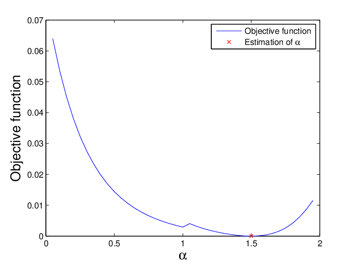
In this example, . Suppose that we have observed the mean residence time for and . Let us find out estimation of by solving the inverse problem of the following nonlocal differential equation:
| (10) | |||
where the generator is
| (11) | |||||
and is the complement set of .
Using the norm, we define an objective function
and the estimation of is taken to be the minimizer, i.e.,
Figure 1 shows accurate estimation of on a smaller domain , as well as on a larger domain .


Example 2.
Consider
| (12) |
.
We estimate , using observation on escape probability . Namely, we solve an inverse problem for the following nonlocal differential equation
| (13) | |||||
| (14) |
where is the generator defined in (2). Defining an objective function
the estimation of is Figure 2 shows the estimation of on two different domains.

Example 3.
Consider
| (15) |
where is a positive parameter.
In this example, we use observations of either mean exit time or escape probability to estimate unknown parameters. Let the observation of mean exit time be and the observation of escape probability be . Defining an objective function
and
respectively, we obtain estimations of parameters by minimizing these functions separately. Results are shown in Figure 3 for using observation of mean exit time and Figure 4 for using observation of escape probability.


4 Discussions and Conclusions
In summary, we have devised a method to estimate the non-Gaussianity parameter , and other system parameters, for non-Gaussian stochastic dynamical systems, using observations on either mean exit time or escape probability. It is based on solving an inverse problem for a deterministic, nonlocal partial differential equation via numerical optimization.
When the noise has a Gaussian component modeled by a Brownian motion , the generator in nonlocal partial differential equations (3) and (6) contains an extra Laplacian term and our method still works. Especially, if the noise has only Gaussian component, the generator is (and the nonlocal term is absent) and our method remains valid.
The existing methods for estimating the non-Gaussianity parameter require observations on system state sample paths for long time periods or probability densities on very large spatial domain. The method proposed here, instead, requires observations on either mean exit time or escape probability only for an arbitrarily small spatial domain. This new method is especially beneficial for systems where either mean exit time or escape probability is relatively easy to observe.
Appendix
In order to solve the numerical optimization problems (5) and (8), we need a numerical scheme to simulate the solutions of (3) and (6) for given initial guesses , respectively. In this Appendix, we only recall a finite difference scheme [12] for solving (3), as a similar scheme works for (6).
Noting the principal value of the integral always vanishes for any , we will choose the value of in Eq. (3) differently according to the value of . Eq. (3) becomes
| (16) |
for ; and for .
Numerical approaches for the mean exit time and escape probability in the SDEs with Brownian motions were considered in [4, 5], among others. In the following, we describe the numerical algorithms for the special case of for clarity of the presentation. The corresponding schemes for the general case can be extended easily. Because vanishes outside , Eq. (16) can be simplified by writing ,
| (17) |
for ; and for .
Noting is not smooth at the boundary points , in order to ensure the integrand is smooth, we rewrite Eq. (17) as
| (18) | |||||
for , and
| (19) | |||||
for . We have chosen .
Let’s divide the interval into sub-intervals and define for integer, where . We denote the numerical solution of at by . Let’s discretize the integral-differential equation (18) using central difference for derivatives and “punched-hole” trapezoidal rule
| (20) |
where . The modified summation symbol means that the quantities corresponding to the two end summation indices are multiplied by .
| (21) |
where . The boundary conditions require that the values of vanish if the index .
The truncation errors of the central difference schemes for derivatives in (20) and (21) are of 2nd-order . The leading-order error of the quadrature rule is , where is the Riemann zeta function. Thus, the following scheme have 2nd-order accuracy for any ,
| (22) |
where . Similarly, for ,
| (23) |
where . if .
We solve the linear system (22-23) by direct LU factorization or the Krylov subspace iterative method GMRES.
We find that the desingularizing term () does not have any effect on the numerical results, regardless whether we use LU or GMRES for solving the linear system. In this case, we can discretize the following equation instead of (17)
| (24) |
where the integral in the equation is taken as Cauchy principal value integral. Consequently, instead of (22) and (23), we have only one discretized equation for any and
| (25) |
Acknowledgement. This work was partly supported by the NSF Grant 1025422. We thank Mike McCourt for help with numerical optimization.
References
- [1] R. J. Adler, R. E. Feldman and M. S. Taqqu (eds.), A Practical Guide to Heavy Tails. Birkhauser, Berlin, 1998.
- [2] D. Applebaum, Lévy Processes and Stochastic Calculus. Cambridge University Press, Cambridge, UK, 2004.
- [3] Yu. Ya Belov, Inverse Problems for Partial Differential Equations. VSP, 2002,
- [4] J. Brannan, J. Duan and V. Ervin, Escape Probability, Mean Residence Time and Geophysical Fluid Particle Dynamics, Physica D 133 (1999), 23-33.
- [5] J. Brannan, J. Duan and V. Ervin, Escape probability and mean residence time in random flows with unsteady drift. Mathematical Problems in Engineering Volume 7 (2001), Issue 1, Pages 55-65. doi:10.1155/S1024123X01001521
- [6] D. Brockmann, Human Mobility and Spatial Disease Dynamics. Chapter in Reviews of Nonlinear Dynamics and Complexity, H. G. Schuster (ed.), Wiley-VCH, 2009.
- [7] Z. Chen, P. Kim and R. Song, Heat kernel estimates for Dirichlet fractional Laplacian. J. European Math. Soc. 12 (2010), 1307-1329.
- [8] P. D. Ditlevsen, Observation of stable noise induced millennial climate changes from an ice record. Geophys. Res. Lett. 26 (1999), 1441-1444.
- [9] H. Ebel, R. Svagera, W. S.M. Werner and M. F. Ebel, Escape Probability of Electrons in Total Electron yield experiments. JCPDS International Centre for Diffraction Data, Vol 41, p.367-378, 1999.
- [10] S. A. Elwakil, E. A. Saad, M. T. Attia and S. K. El-Labany, Particle escape probability from spherical geometry. Astrophysics and Space Science Volume 150, Number 1 (1988), 9-15.
- [11] R. G. Forbes, On the need for a tunneling pre-factor in FowlerNordheim tunneling theory. Journal of Applied Physics 103 (11)(2008): 114911.
- [12] T. Gao, J. Duan, X. Li and R. Song, Mean exit time and escape probability for dynamical systems driven by Lévy noise. Submitted to SIAM J. Sci. Comput. arXiv:1201.6015v1 [math.NA].
- [13] F. Ghirelli and B. Leckner, Transport equation for the local residence time of a fluid. Chemical Engineering Science 59 (2004) 513-523.
- [14] Y. Hu and H. Long, Parameter estimation for Ornstein-Uhlenbeck processes driven by -stable Lévy motions. Communications on Stochastic Analysis, 2007, 1: 175-192.
- [15] Y. Hu and H. Long, Least squares estimator for Ornstein-Uhlenbeck processes driven by -stable motions. Stochastic Process Appl, 2009, 119: 2465-2480.
- [16] N. E. Humphries, H. Weimerskirch, N. Queiroz, E. J. Southall and D. W. Sims, Foraging success of biological Lévy flights recorded in situ, Proc. Natl. Acad. Sci. 109(19):7169-7174 (2012)
- [17] I. A. Ibragimov and R. Z. Has’minskii, Statistical Estimation—Asymptotic Theory. Springer, New York, 1981.
- [18] V. Isakov, Inverse Problems for Partial Differential Equations. Springer, New York, 1998.
- [19] A. Janicki and A. Weron, Simulation and Chaotic Behavior of Stable Stochastic Processes, Marcel Dekker, Inc., 1994.
- [20] A. Kirsch, An Introduction to the Mathematical Theory of Inverse Problems. Springer, New York, 1996.
- [21] H. Long and L. Qian, Nadaraya-Watson estimator for stochastic processes driven by stable Lévy motions. Electronic Journal of Statistics, Vol. 7 (2013) 13871418
- [22] F. Moss and P. V. E. McClintock (eds.), Noise in Nonlinear Dynamical Systems. Volume 1: Theory of Continuous Fokker-Planck Systems (2007); Volume 2: Theory of Noise Induced Processes in Special Applications (2009); Volume 3: Experiments and Simulations (2009). Cambridge University Press.
- [23] T. Naeh, M. M. Klosek, B. J. Matkowsky and Z. Schuss, A direct approach to the exit problem, SIAM J. Appl. Math. 50 (1990), 595-627.
- [24] E. B. Nauman, Residence Time Distributions. In Handbook of Industrial Mixing: Science and Practice. Wiley Interscience, pp. 117 (2004).
- [25] J. A. Novotny, E. C. Parker, S. S. Sruvanshi, G. W. Albin and L. D. Homer, Contribution of tissue lipid to long xenon residence times in muscle. J Appl Physiol. 1993 May;74(5):2127-34.
- [26] B. Oksendal, Applied Stochastic Control Of Jump Diffusions. Springer-Verlag, New York, 2005.
- [27] H. Qiao, X. Kan and J. Duan, Escape probability for stochastic dynamical systems with jumps. Springer Proceedings in Mathematics & Statistics, Vol. 34, p. 195-216, 2013.
- [28] G. Samorodnitsky and M. S. Taqqu, Stable Non-Gaussian Random Processes, Chapman and Hall, 1994.
- [29] K.-I. Sato, Lévy Processes and Infinitely Divisible Distributions, Cambridge University Press, Cambridge, 1999.
- [30] D. Schertzer, M. Larcheveque, J. Duan, V. Yanovsky and S. Lovejoy, Fractional Fokker–Planck equation for nonlinear stochastic differential equations driven by non-Gaussian Lévy stable noises. J. Math. Phys., 42 (2001), 200-212.
- [31] M. F. Shlesinger, G. M. Zaslavsky and U. Frisch, Lévy Flights and Related Topics in Physics (Lecture Notes in Physics, 450. Springer-Verlag, Berlin, 1995).
- [32] T. H. Solomon, E. R. Weeks, and H. L. Swinney, Observation of anomalous diffusion and Lévy flights in a two-dimensional rotating flow. Phys. Rev. Lett. 71, 3975 - 3978 (1993).
- [33] W. A. Woyczynski, Lévy processes in the physical sciences. In Lévy Processes: Theory and Applications, O. E. Barndorff-Nielsen, T. Mikosch and S. I. Resnick (Eds.), 241-266, Birkhäuser, Boston, 2001.
- [34] J. Yang and J. Duan, Quantifying model uncertainties in complex systems. Progress in Probability, Vol. 65, p.49-80, 2011.