Recursive Sorting in Lattices

If someone asked whether there is for the numbers $x$ and $y$ and the exponent $n$ a general relationship between the value $(x+y)^{n}$ and the powers $x^{n}$ and $y^{n}$, then the (obvious) answer is that this relationship is captured by the Binomial Theorem

which also shows that other powers of $x$ and $y$ are involved.

If, on the other hand, $(x_{1},\ldots,x_{n})$ is a sequence in a totally ordered set $(X,\leq)$ and someone asked whether there is a general relationship between the elements of $x$ and the elements of its nondecreasingly sorted counterpart ${x}^{\uparrow}=\left({x}^{\uparrow}_{1},\ldots,{x}^{\uparrow}_{n}\right)$, then one could provide an easy answer for the first and last elements of ${x}^{\uparrow}$. In fact, we know that ${x}^{\uparrow}_{1}$ is the least element of $\{x_{1},\ldots,x_{n}\}$

The relationship between an arbitrary element ${x}^{\uparrow}_{k}$ and the elements of $x$ reads

and has been proven in a previous work of the author [1, Proposition 2.2]. Here $\mathbb{N}\tbinom{n}{k}$ is the set of subsets of $[1,n]$ that contain exactly $k$ elements. Note that $\mathbb{N}\tbinom{n}{k}$ consists of $\tbinom{n}{k}$ elements.

Equation (1) is not just a compact formula for computing ${x}^{\uparrow}$. It also provides a way to generalize the concept of sorting beyond totally ordered sets. In fact, if $(X\leq)$ is a partically ordered set, that is also a lattice $(X,\wedge,\vee)$, then for each finite subset $A$ of $X$ both the infimum and supremum of $A$ exist (denoted by $\bigwedge A$ and $\bigvee A$, respectively). Thus, the right hand side of Equation (1) is well-formed in a lattice. Therefore we can define (as in [1, Definition 3.1]) for $x=(x_{1},\ldots,x_{n})$ a new sequence ${x}^{\vartriangle}=\left({x}^{\vartriangle}_{1},\ldots,{x}^{\vartriangle}_{n}\right)$ by

We refer to ${x}^{\vartriangle}$ as $x$ sorted with respect to the lattice $(X,\wedge,\vee)$. It can be shown that this definition of sorting in lattices maintains many properties that are familiar from sorting in totally ordered sets. For example, the sequence $\left({x}^{\vartriangle}_{1},\ldots,{x}^{\vartriangle}_{n}\right)$ is nondecreasing [1, Lemma 2.3] and the mapping $x\mapsto{x}^{\vartriangle}$ is idempotent [1, Lemma 3.6].

Note that we reserve the notation ${x}^{\uparrow}$ in order to refer to sorting in totally ordered sets whereas we use the notation ${x}^{\vartriangle}$ to refer to sorting in lattices.

Definition (2) is nice and succinct, but it is also are quite impractical to use in computations. While conducting some experiments with Equation (2) in the lattice $(\mathbb{N},\gcd,\operatorname{\mathrm{lcm}})$ it became obvious that only for very short sequences $x$ the sequence ${x}^{\vartriangle}$ can be computed in a reasonable time.

Table 1 shows simple performance measurements (conducted on a notebook computer) for computing ${(1,\ldots,n)}^{\vartriangle}$ in $(\mathbb{N},\gcd,\operatorname{\mathrm{lcm}})$. The reason for this dramatic slowdown is of course the exponential complexity inherent in Equation (2): In order to compute ${x}^{\vartriangle}$ from $x$ it is necessary to consider all $2^{n}-1$ nonempty subsets of $[1,n]$.

In order to address this problem, we prove in Proposition 1 the recursive Identity (8) for the case of bounded distributive lattices. This identity is closely related to the well-known fact that the binomial coefficient

Furthermore, we prove in Proposition 2 that a lattice, in which Identity (8) holds, is necessarily distributive.

For the remainder of this paper we assume that $(X,\wedge,\vee,\bot,\top)$ is a bounded lattice. Here $\bot$ is the least element of $X$ and the neutral element of join

We are now introducing a notation that allows us to concisely refer to individual elements of both ${(x_{1},\ldots,x_{n})}^{\vartriangle}$ and ${(x_{1},\ldots,x_{n-1})}^{\vartriangle}$. Here again, it is convenient to employ the symbol for the binomial coefficient $\tbinom{n}{k}$ in the context of sorting in lattices.

For a sequence $x$ of length $n$ we define for $0\leq m\leq n$

We know from the definition of ${x}^{\vartriangle}$ in Equation (2) that

holds for $1\leq k\leq n$.

The main result of this paper is Proposition 1, which states in Identity (8), how the $k\text{th}$ element of ${(x_{1},\ldots,x_{n})}^{\vartriangle}$ can be computed from ${(x_{1},\ldots,x_{n-1})}^{\vartriangle}$ and $x_{n}$ by simply applying one join and one meet.

The proof of Proposition 1 relies on the fact that the lattice under consideration is both bounded and distributive. The boundedness of $X$ is, in contrast to its distributivity, no real restriction because every lattice can be turned into a bounded lattice by adjoining a smallest and a greatest element [2, p. 7].

The following Proposition 2 states that the converse of Proposition 1 also holds.

Using Identity (8), we can prove following Lemma 3, which generalizes a known fact known from sorting in a total order: If one knows that $x_{n}$ is greater or equal that the preceding elements $x_{1},\ldots,x_{n-1}$ then sorting the sequence $(x_{1},\ldots,x_{n})$ can be accomplished by sorting $(x_{1},\ldots,x_{n-1})$ and simply appending $x_{n}$.

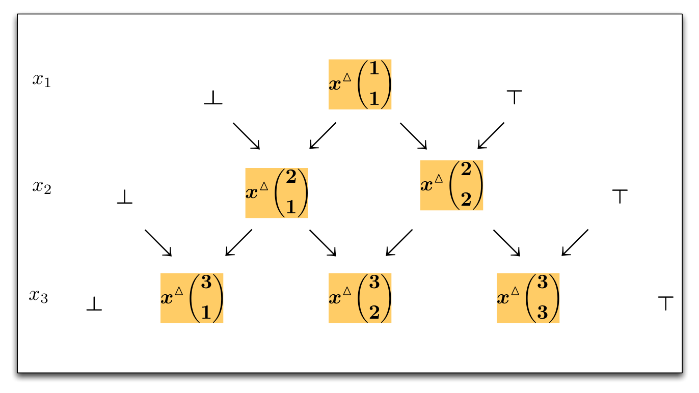
Equation (4) symbolically represents Identity (8). Whenever an arrow $\searrow$ and and arrow $\swarrow$ meet, the values are combinedby a meet. In the case of an arrow $\searrow$, however, first the value at the origin of the arrow is combined with the sequence value $x_{n}$ through a join.

Figure 2 integrates several instance of Equation (4) in order to graphically represent Identity (8) and to emphasize its close relationship to Pascal’s triangle.

Figure 3 outlines an algorithm, which is based on Identity (8), and that starting from ${(x_{1})}^{\vartriangle}=(x_{1})$ successively computes ${(x_{1},\ldots,x_{i})}^{\vartriangle}$ for $2\leq i\leq n$.

From Identity (8) follows that in step $i$ exactly $i$ joins and $i$ meets must be performed. Thus, altogether there are

applications of join and meet. In other words, such an implementation has quadratic complexity. The algorithm in Figure (3) can be considered as insertion sort [3, § 5.2.1] for lattices because one element at a time is added to an already “sorted” sequence.

Table 2 shows the results of performance measurements in the bounded and distributive lattice $(\mathbb{N},\gcd,\operatorname{\mathrm{lcm}},1,0)$. Here, we are using an implementation that is based on the algorithm in Figure (3).

These results show that sorting in lattices can now be applied to much larger sequences than those shown in Table (1) before the limitations of an algorithm with quadratic complexity become noticeable.

The main results of this paper are Proposition 1 that proves Identity (8) for bounded distributive lattices and Proposition 2 that shows the necessity of the distributivity for Identity (8) to hold.

The remarkable points of Identity (8) are that it exhibits a strong analogy between sorting and Pascal’s triangle, allows to sort in lattices with quadratic complexity, and is in fact a generalization of insertion sort for lattices.

I am very grateful for the many corrections and valuable suggestions of my colleagues Jochen Burghardt and Hans Werner Pohl.

In particular, Jochen Burghardt’s suggestion to investigate whether the distributivity in Proposition 1 is really necessary led to Proposition 2. Hans Werner Pohl pointed out the analogy of the algorithm in Figure 3 to insertion sort.

References

• [1] J. Gerlach. Sorting in Lattices. ArXiv e-prints, March 2013.
• [2] S. Roman. Lattices and Ordered Sets. Springer-Verlag New York, 2008.
• [3] Donald E. Knuth. The Art of Computer Programming, Volume III: Sorting and Searching. Addison-Wesley, 1973.