Improving photon-hadron discrimination based on cosmic ray surface detector data
Abstract
The search for photons at EeV energies and beyond has considerable astrophysical interest and will remain one of the key challenges for ultra-high energy cosmic ray (UHECR) observatories in the near future. Several upper limits to the photon flux have been established since no photon has been unambiguously observed up to now. An improvement in the reconstruction efficiency of the photon showers and/or better discrimination tools are needed to improve these limits apart from an increase in statistics. Following this direction, we analyze in this work the ability of the surface parameter , originally proposed for hadron discrimination, for photon search.
Semi-analytical and numerical studies are performed in order to optimize for the discrimination of photons from a proton background in the energy range from to eV. Although not shown explicitly, the same analysis has been performed for Fe nuclei and the corresponding results are discussed when appropriate. The effects of different array geometries and the underestimation of the muon component in the shower simulations are analyzed, as well as the dependence on primary energy and zenith angle.
Keywords:
Cosmic Rays , Photon Discrimination , Cherenkov Detectors , parameter1 Introduction
Photons at EeV energies and higher are thought to be typically produced as decay secondaries in our cosmological neighborhood. They come from higher-energy cosmic rays (nucleon or nucleus) that interact with matter or background photons producing neutral pions and neutrons. A typical case is the Greisen, Zatsepin and Kuzmin (GZK) process (see e.g. Ref. [1]) where a proton above EeV interacts with the cosmic microwave background (CMB) photons losing energy and, in the most probable case, producing a neutral pion that almost immediately decay into 2 photons of about each of the initial proton energy. Neutrons could also be produced in the GZK interaction with of the initial energy and later decay producing an electron and a new proton with around and of the neutron energy respectively. If the initial proton energy is , the secondary electron could finally produce a photon of EeV energies through inverse Compton. Also, if UHE photons are generated in cosmologically distant sources, the flux is expected to steepen above the energy threshold of the GZK process since their attenuation length is only of the order of a few Mpc at such high energies.
The AGASA Collaboration on the other hand, reported a flux of UHECRs with no apparent steepening above [2]. Motivated by these measurements, many theoretical models were proposed that are able to create particles of the observed energy at relatively close distances from the Earth. These models involve super heavy dark matter (SHDM), topological defects, neutrino interactions with the relic neutrino background (Z-bursts), etc. These are called top-down models since the UHE particle is a consequence of the decay or annihilation of a more energetic entity (see Ref. [3] for a review). A key signature of these models is a substantial photon flux at the highest energies. Thus, the search for UHE photons was highly stimulated. Recently, the suppression in the spectrum has been confirmed by Auger [4] and HiRes [5], but its origin is still unknown and compatible with a subdominant contribution of these top-down models.
The present status is that no observation of photons has been claimed above eV by any experiment. The main candidates reported by both older experiments, like AGASA [6] and Yakutsk [7], or the newer Pierre Auger Observatory (Auger hereafter) [8] and Telescope Array (T.A.) [9], are all compatible with the expected fluctuations of a pure sample of very deep proton shower events. The most stringent upper limits to the photon flux have been established by Auger (, , , , for energy above , , , , EeV using hybrid data [10] and, , , for energy above , , EeV using surface data [8]) .
Despite the fact that no photons have been unambiguously identified up to now, a relatively small fraction of photons in the primary flux cannot be ruled out, and their detection would have profound implications in our understanding of the nature and origin of UHECRs. In fact, recent upper limits in the photon fraction constrain SHDM models in such a way that cosmic rays originated in these scenarios could only contribute in a subdominant way to the total flux. In addition, these limits are close to the predicted photon flux caused by the GZK interaction in certain models, whose detection would support the extragalactic origin of UHECRs and bring independent clues on their composition (see Ref. [11] for a review). Also, more stringent limits on EeV photons reduce corresponding systematic uncertainties in the reconstruction of the energy spectrum [12] and the derivation of the proton-air cross-section [13], and affect the interpretation of the observed elongation rate [14].
Auger and the Telescope Array are the experiments that can currently detect EeV photons. Both are hybrid observatories with a ground array of detectors and fluorescence telescopes. At these energies, cosmic rays interact with Earth’s atmosphere producing extensive air showers (EAS). EAS initiated by photon primaries are expected to develop deeper in the atmosphere compared to hadrons, producing larger values of , the maximum of shower development measurable by the fluorescence telescopes. On the other hand, the surface detector exploits the fact that photon showers are characterized by a smaller number of secondary muons and a more compact footprint at ground. Several observables have been applied to surface data, mainly related with the spatial and temporal structure of the shower front at ground [8, 9]. A new surface parameter, called , was proposed for proton-iron discrimination in Ref. [15]. It is sensitive to the combined effects of the different muon and electromagnetic components on the lateral distribution function. In this work, we optimize for photon searches and analyze its specific properties for photon primaries.
The energy calibration with the surface detector is different for hadron and photon primaries, so the calculation of an upper photon limit from pure surface information is a complex issue. The interpolated signal at a certain distance to the shower axis is used as energy estimator ( in Auger [4] and in Telescope Array [16]) for both primaries but, comparing hadron and photon showers of the same primary energy and zenith angle, the difference in the energy estimator is about a factor of above eV, on average. Therefore, while the energy calibration for hadron primaries is done by using hybrid events, i.e. events seen by the fluorescence telescopes and the surface detectors simultaneously, pure Monte Carlo (MC) methods are used in case of photon-induced showers (see Ref. [8, 17] for Auger and Ref. [9] for T.A.). This energy scale difference is unavoidable for surface detector alone since it is a consequence of the different physics involved in hadron and pure electromagnetic showers. An unbiased measurement of the energy is possible if only hybrid events are used, since the primary energy is directly obtained from the longitudinal profile measured by the fluorescence telescopes. We assume here that the primary energy is the one used to simulate the showers (MC energy) since the problem of the different energy scales for pure surface events is beyond the scope of this work.
2 Semi-analytical calculation
In this section an improved version of the semi-analytical calculation developed in Ref. [15] is introduced, in order to more deeply understand the behavior of the parameter.
The parameter [15], is defined as,
| (1) |
where the sum extends over all triggered stations N, is a reference distance ( m in the case of Auger), is the signal measured in the th station, and is the distance of this station to the shower axis.
The discrimination power between protons () and photons () of the parameter can be estimated by using a merit factor defined as,
| (2) |
where and are the mean value and the variance of , respectively, with .
The calculation of the merit factor of corresponding to protons and photons, by using a semi-analytical approach, requires the knowledge of the lateral distribution function (LDF), the signal as a function of the distance to the shower axis, for both protons and photons. Figure 1 shows the LDFs, obtained from simulations of the showers impinging on Auger water Cherenkov surface detectors (see section 3.2 for details), corresponding to proton and photon primaries of energy in the interval eV and zenith angle , such that , i.e. . Also shown are the LDFs corresponding to muons and to the electromagnetic particles (mainly electrons, positrons and photons). Solid lines correspond to the fits of the simulated data with a NKG-like function [18],
| (3) |
where m and m, and , and are free fit parameters. For the fits of the LDFs corresponding to the total and electromagnetic signal, the condition is used, i.e. is considered as a free parameter just for the fit corresponding to the muon signal.


As expected, from figure 1 it can be seen that the muon component of the photon showers is much smaller than the corresponding one to protons.
Following Ref. [15] the distribution function for a given configuration of distances to the shower axis and signals (in a given event) can be written as,
| (4) | |||||
where is the distance to the shower axis of the th station (the first station, , is the closest one) and is the average LDF evaluated at . Note that, in this case, the Gaussian distribution corresponding to the deposited signal in each station used in Ref. [15] is replaced by a Poissonian distribution which is more suitable for small values of the total signal. Here is the distribution function of the random variables with , which depends on the incident flux and the geometry of the array.
From the definition of and Eq. (4) the following expressions for the expectation value and the variance of are obtained,
| (5) | |||||
| (6) | |||||
where
| (7) | |||||
| (8) |
see Ref. [15] for details. Here and correspond to the mean value of and respectively,
| (9) | |||||
| (10) |
where it is assumed that the stations included in the calculation are such that , where corresponds to a trigger condition and to a saturation level. Taking VEM and assuming that for the Poissonian distribution can be approximated by a Gaussian, the following expressions are obtained,
| (11) | |||||
| (12) | |||||
where
| (13) |
Following Ref. [20] it is assumed that VEM.
The calculation of the expectation value and the variance of for proton and photon primaries requires the knowledge of the distribution function which is very difficult to obtain analytically. Therefore, a very simple Monte Carlo simulation is used instead. A triangular grid of m of distance between detectors, like the one corresponding to Auger, is first considered. The impact points are distributed uniformly in the central triangle of the array and the arrival directions of the primaries are simulated following an isotropic flux such that .
The merit factor is calculated from Eqs. (2,5,6), the fitted proton and photon LDFs and the position of the stations obtained from the Monte Carlo simulations. Figure 2 shows the comparison between the merit factor as a function of , obtained by using the semi-analytical approach and a simplified Monte Carlo simulation, proposed in Ref. [20] and also tested in Ref. [15], which includes the simulation of the impact points of the showers, the arrival direction and also the Poissonian fluctuations of the signal in each station. Note that the proton and photon LDFs used in both calculations are the same. From the figure, it can be seen that, as expected, as a function of obtained from the two different methods are in very good agreement. Also note that the maximum value of is obtained for , very close to .

2.1 Influence of fluctuations on the discrimination power of
The discrimination power of is dominated by two type of fluctuations, the ones corresponding to the distance of the stations to the shower axis, which come from the uniform distribution of the impact points of the showers over the array area, and the ones originated by the detection of the particles that reach a given station, i.e. signal fluctuations.
The semi-analytical approach allow us to isolate the contributions of the different sources of fluctuations that generate the maximum of the curve of as a function of . Let us consider the case in which we freeze a realization of the spatial distributions of the stations with respect to the shower core position, then Eqs. (5,6) become,
| (14) | |||||
| (15) |
where is the expectation value of the distance to the shower axis of the th station. Line labeled as (a) of figure 3 corresponds to as a function of calculated under this approximation. It can be seen that decreases for increasing values of . The signal corresponding to the stations that are far from the shower axis presents larger fluctuations, therefore, when increases, the weight of these stations also increases making to decrease.

Let us consider the other important case in which the fluctuations of the signal are switched off. In this case Eqs. (5,6) become,
| (16) | |||||
| (17) |
where
| (18) |
Line labeled as (b) of figure 3 corresponds to as a function of calculated by using Eqs. (16,17). It can be seen that for small and for large values of , is small. For values of close to zero the most important contribution to comes from the signal of the station closest to shower core. Therefore, due to the fast variation of the LDF with the distance to the shower axis, the fluctuations on the position of the first station are translated into very large fluctuations of the signal, decreasing drastically the discrimination power of . The same happens for larger values of but in this case the farthest station is the important one.
Note that the dominant effect for the increase of in the regions of where the curves (a) and (b) differ significantly from the exact value comes from the decrease of the variance. For the case in which the fluctuations on the positions of the stations are frozen the difference between the mean values is larger than the exact one for small values of . However in the case where the signal fluctuations are frozen the difference between the mean values is smaller than the exact one for large values of .
Also note that comparing the expression of the variance for the two cases considered, Eqs. (15) and (17), with the exact expression, Eq. (6), it can be seen that the first term of the variance for the exact case has to do with the signal fluctuations and the second one with the fluctuations on the distance of the stations to the shower axis.
Line labeled as (c) in the figure 3 corresponds to the calculation of in which the variance of Eq. (6) is calculated by just considering the first term. It can be seen that, for values of larger than the corresponding to the maximum, this term is dominated by the fluctuations of the signal. Line labeled as (d) in the figure corresponds to the calculation of in which the variance of Eq. (6) is calculated by just considering the second term. In this case it can be seen that from up to values close to the maximum, the behavior of is dominated by the fluctuations on the position of the stations combined with the fast variation of the LDFs with . Therefore, the formation of the maximum in as a function of appears due to these two effects. Note that, the fluctuations on the position of the stations also contribute to the calculation of corresponding to line (c) and the fluctuations on the signal also contribute to the calculation of corresponding to the line (d), i.e. the exact value of the maximum cannot be obtained by just combining the cases in which these two kind of fluctuations are isolated.
2.2 Modifying the muon content of showers
There is experimental evidence about a deficit in the muon content of the simulated showers [21, 22, 23]. The hadronic interaction models at the highest energies cannot completely describe the observations. Therefore, the muon content of the showers is modified artificially, in order to study its influence on the discrimination power of . For that purpose, the LDFs corresponding to the total signal, for both protons and photons, are obtained combining the fits of the LDFs corresponding to the electromagnetic and muon components (see figure 1) in such a way that, , where corresponds to the prediction of QGSJET-II. Figure 4 shows as a function of for different values of , from to in steps of . It can be seen that the maximum value reached by increases with . This is due to the fact that the difference between the mean value of for protons and the corresponding one to photons increases with , as in the case of proton and iron primaries (see Ref. [15] for details). Also, when increases the total signal increases, reducing the fluctuations of the parameter. Note that, , the value that maximize decreases with going from for to for .

3 Shower and detector simulations
In this Section detector simulations are performed in order to analyze the most relevant properties of the parameter. For the calculation of , at least triggered stations in the event are needed to assure the geometrical reconstruction of the shower axis. Therefore, the efficiency, i.e. the fraction of events that fulfills this requirement, is almost above the energy threshold of the corresponding array, highlighting a major advantage of the parameter. In a real experiment no quality cut on is needed except that it could be convenient to require a minimum number of active (not necessarily triggered) detectors during the event (for example were imposed in Ref. [10]) or to examine individually the few events selected as photon candidates to avoid a possible underestimation of due to a missing or non-operating station which would mimic the behavior of a primary photon.
3.1 optimization for different array sizes and geometries
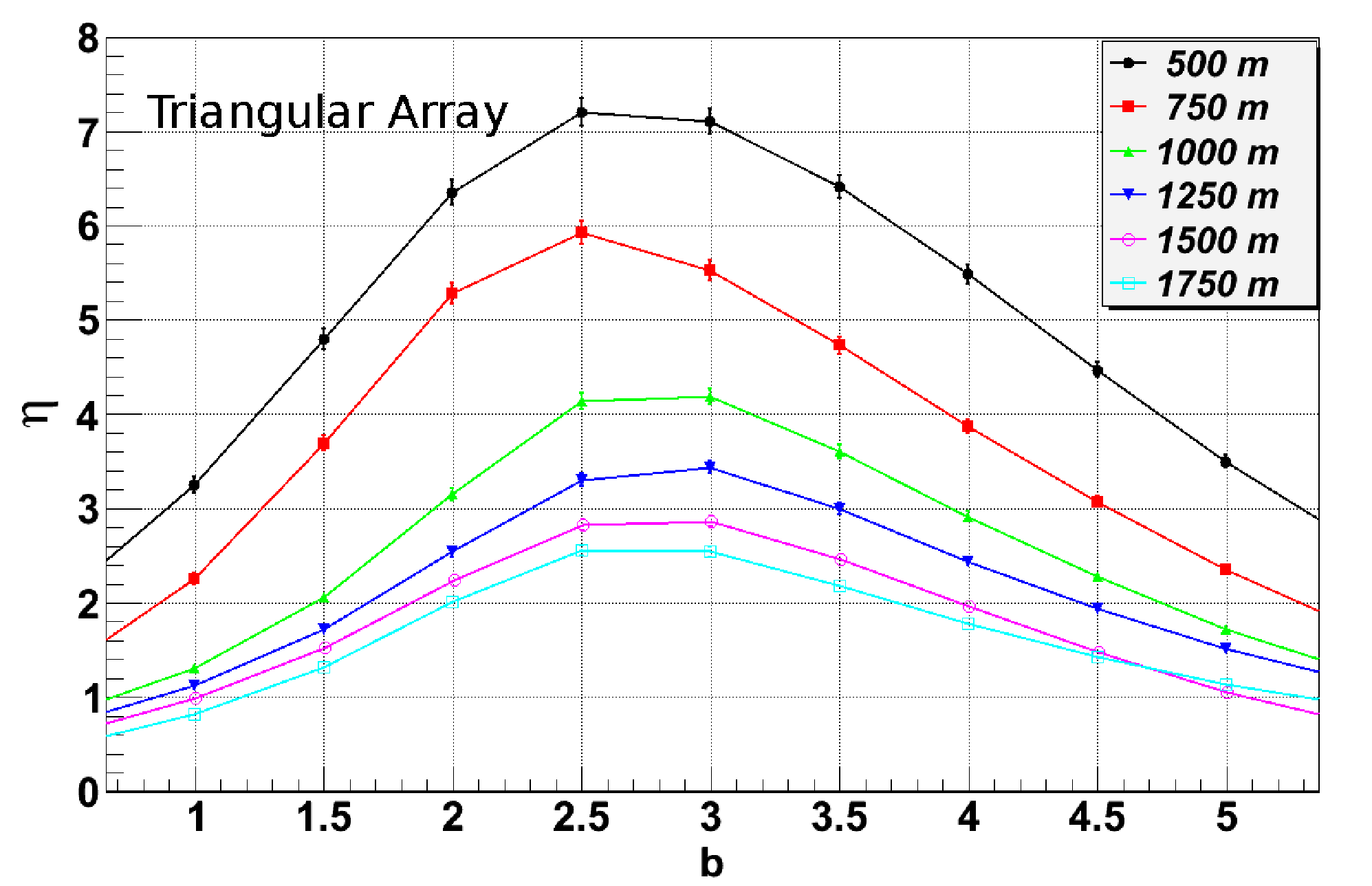
The detection of the extensive air showers by a surface array of water Cherenkov tanks is here simulated by using our own simulation program described previously in Section 2 and Ref. [20]. The geometry of the array and the distance between detectors are easily modified in order to study their effect on . Thus, triangular and square grids are considered varying the array spacing from to meters.
The error in the merit factor, , is calculated assuming Poissonian errors and is given by,
| (19) |
where and are the number of events in each population (here are used).
Figure 5 shows the merit factor as a function of for different array sizes corresponding to a triangular and square grids. increases as the array spacing decreases as expected, since the LDF is sampled in more points as the array becomes denser. is slightly larger for the triangular grid since the number of triggered stations is also larger for this geometry. is the optimum value for most of the arrays considered, independent of the geometry.

3.2 More realistic simulations
In what follows, we perform a more realistic simulation in order to treat more accurately the tank response and to take into account the shower to shower fluctuations and experimental uncertainties such as the shower reconstruction.
The simulation of the atmospheric showers is performed with the AIRES Monte Carlo program (version 2.8.4a) [24] with either QGSJET-II-03 or [19] Sibyll 2.1 [25] as the hadronic interaction model (HIM). The simulation of the tank response and the shower reconstruction are performed with the Offline Software provided by the Pierre Auger Collaboration [26]. The simulation is done for a triangular grid of water Cherenkov detectors of km of spacing, as in Auger.
The primary energy goes from to in steps of . events are simulated per each HIM and energy bin. The zenith angle follows an isotropic distribution from to while the azimuth is selected randomly from a uniform distribution in the interval from to .
The library called MaGICS [27] can be linked to AIRES in order to simulate the conversion of photons in the geomagnetic field. However, we do not have to deal with photon splitting, because only a negligible fraction of inclined showers convert at most latitudes of interest below 50 EeV [28].
The results are very similar for both HIM, so most are only shown for QGSJET-II-03 unless otherwise stated.
3.3 optimization for in and in
The value of that maximizes the merit factor as a function of the logarithm of the primary energy, , is shown in figure 6 for three zenith angle bins. In case of vertical showers with , in agreement with the semi-analytical calculation (figure 2). In the bottom panel, the bands that represent a variation in are added showing the reliability of as a discriminator, even for a non-optimal selection of the index .
From figure 7 it can be seen that for all energies and zenith angles analyzed, except for low energy primaries in the small range with (). Therefore, we conclude that is an optimum choice for the whole energy and zenith angle ranges analyzed, maintaining the simplicity of the parameter.
Although the merit factor is a good parameter to measure the statistical discrimination power of a variable, it carries by itself few information on the existence, shape and strength of tails of the distribution functions of the parameters. Since those tails can be also important from the point of view of the definition and understanding of the quality cuts, we include in figure 8 an example of the distribution functions for protons and photons in the energy range from and 1.00 1.33, where it can be seen that photon tails with proton-like behavior are statistically negligible but do exist.
Despite the fact that only protons have been considered so far in the analysis, a sizable fraction of heavier nuclei cannot be discarded at the highest energies [14]. However, although not shown in this paper for brevity, equivalent calculations considering a pure iron composition show that for photon-iron discrimination is larger than for photon-proton discrimination. Therefore, , particularized for , can be used in general for photon-hadron discrimination with similar, or even better results, regardless of the exact UHECR mass composition.


3.4 dependence with primary energy and zenith angle
Figure 9 shows the relation between and the primary energy. An almost linear relation is found, in agreement with Ref. [15] where only hadrons were considered. Note that the result is almost independent of the hadronic interaction model and that the slope is smaller for photons compared to hadrons.

The dependence of with the zenith angle of the incoming shower for primary photons is quite complex, as shown in the top panel of figure 10. While the dependence with is stronger as the energy increases, the shape is similar, showing a maximum that slowly increases from to over a decade of energy.
The dependence of can be qualitatively understood by considering a simplified physical situation. Let us assume that the LDF follows a power-law, , where m and is the slope. If , then , where is the number of candidate stations. The dependence of with zenith angle is shown in the bottom panel of figure 10. is expected to increase with since the shower footprint at ground becomes larger and more elongated. On the other hand, decreases with due to the larger attenuation in the atmosphere. The combination of these two effects roughly explain the existence of this maximum.


In the case of hadrons, has in general a small dependence on zenith angle, which is more manifest for quasi vertical showers at the lowest energies (c.f., [15]). In any case, as it is shown in figure 11, such a dependence does not hinder the discrimination power of the parameter, unless the error in energy estimate is unrealistically large ( or ).


4 Conclusions
We have applied the proposed parameter, obtained from the information given by an array of water Cherenkov detectors, to photon-hadron discrimination. By means of an improved semi-analytical calculation we have shown that, as in the case of proton-iron discrimination, there is a well defined value of the exponent that maximizes its discrimination capability. We have found that at eV the optimum value of the exponent is . We have demonstrated that the fluctuations on the position of the stations, combined with the very fast variation of the LDFs with distance, are responsible for the decrease of the merit factor at small values of . On the other hand, we have shown that the fluctuations of the signal measured in each station are dominant at large values of , decreasing the merit factor in this range. Therefore, the maximum of is attained in the transition between these two regimes.
Experimental data suggest an excess of muons in the showers with respect to the prediction of current hadronic interaction models. By means of the semi-analytical calculation we have studied the effects on the discrimination power when the muon content of the showers is modified. We have found that, the optimal value of the exponent is still close to when the muon content of the showers is modified and that the discrimination power of is actually enhanced when the muon content of the showers increases.
This result is generalized by using two complementary and independent approaches. First, using our own simple MC program [20] of the shower detection and reconstruction, we have demonstrated that is the value that maximizes the merit factor for many different arrays, varying the geometry (triangular and square unitary cells) and the distance between detectors for a large range of separations (from to m). Second, using a set of full numerical simulations, with a realistic tank response and taking into account the shower to shower fluctuations and experimental uncertainties, we have demonstrated that is close to the optimum value in the whole energy range from to eV and zenith angles from to . Furthermore, we have also shown that the discrimination power of is not significantly affected even if a suboptimal value of is used.
Additionally, since the UHECR flux likely includes a sizable fraction of heavier primaries besides protons, the same analysis has been performed assuming the opposite scenario, i.e. a pure iron background. The discrimination power of is even larger in this case, confirming the fact that can be used as a composition discriminator regardless of the exact hadron composition.
We have demonstrated that is almost linearly dependent on the primary energy. The zenith angle dependence for photon primaries has been qualitatively understood in terms of the evolution of the number of triggered stations and with the primary zenith angle. In the case of hadrons, has in general a small dependence on zenith angle which does not hinder the discrimination power of the parameter, unless the error in energy estimate is unrealistically large ( or ).
The calculation of an upper photon limit from pure surface information is a great challenge since, as commented previously, the energy reconstruction method introduces a composition-dependent bias. This problem could be overcome if only hybrid events are considered. Then, our results suggest that combined with fluorescence observables (mainly as in Ref. [10]) could improve the upper limits to the photon flux in the whole energy range of the experiments with a unified treatment since is almost full-efficient above the energy threshold of the corresponding array with a large discrimination power.
5 Acknowledgments
All the authors have greatly benefited from their participation in the Pierre Auger Collaboration and its profitable scientific atmosphere. Extensive numerical simulations were made possible by the use of the UNAM super-cluster Kanbalam and the UAH-Spas cluster at the Universidad de Alcalá. We want to thank the Pierre Auger Collaboration for allowing us to use the Auger Offline packages in this work, C. Bleve and B. Zamorano for fruitful discussions and J. A. Morales de los Ríos for the maintenance of the UAH-Spas cluster. We also thank the support of the MICINN Consolider-Ingenio 2010 Programme under grant MultiDark CSD2009-00064, Astomadrid S2009/ESP-1496, and EPLANET FP7-PEOPLE-2009-IRSES.
This work is partially supported by Spanish Ministerio de Educación y Ciencia under the projects FPA2009-11672, Mexican PAPIIT-UNAM through grants IN115707-3, IN115607, IN115210 and CONACyT through grants 46999-F, 57772, CB-2007/83539. ADS is member of the Carrera del Investigador Científico of CONICET, Argentina.
References
- [1] G. Gelmini, O. Kalashev, D.V. Semikoz, J. Exp. Theor. Phys. 106 (2008) 1061–1082.
- [2] N. Hayashida et al., Phys. Rev. Lett. 73 (1994) 3491.
- [3] P. Bhattacharjee, G. Sigl, Phys. Rep. 327 (2000) 109–247. Available from: astro-ph/9811011.
- [4] The Pierre Auger Collaboration, Physics Letters B 685 (2010) 239–246.
- [5] Bingkai Zhang et al. Nucl.Phys.Proc.Suppl. 175-176 (2008) 241-244.
- [6] K. Shinozaki et al., Astrophys. J. 571, (2002) L117.
- [7] A. V. Glushkov et al., Phys. Rev. D82, (2010) 041101.
- [8] The Pierre Auger Collaboration. Astropart. Phys. 29, (2008) 243-256.
- [9] G. Rubtsov, et al. [Telescope Array Collaboration], Proc. 32nd ICRC, Beijing, China, 2011.
- [10] M. Settimo, for the Pierre Auger Collaboration. Proc. 32nd ICRC. Beijing, China, 2011. Available from: arXiv:1107.4805.
- [11] J. Alvarez-Muniz and M. Risse [Pierre Auger Collaboration], G.I. Rubtsov and B.T. Stokes [Telescope Array Collaboration]. UHECR International Symposium, CERN, 2012. Available at EPJ Web of Conferences.
- [12] N. Busca, D. Hooper, E.W. Kolb, Phys. Rev. D 73 (2006) 123001. Available from: astro-ph/0603055.
- [13] The Pierre Auger Collaboration, Phys. Rev. Lett. 109, (2012) 062002.
- [14] The Pierre Auger Collaboration. Phys.Rev.Lett. 104 (2010) 091101.
- [15] G. Ros et al., Astropart. Phys. 35, (2011) 140.
- [16] Telescope Array Collaboration. Available from: arXiv:1205.5067.
- [17] P. Billoir, C. Roucelle, J.C. Hamilton. arXiv:astro-ph/0701583.
- [18] K. Greisen, Progress in Cosmic Ray Physics, vol. 3, 1956.
- [19] S. Ostapchenko, Nucl. Phys. Proc. Suppl. B151 (2006) 143.
- [20] G. Ros et al., Nucl. Instrum. Meth. A608 (2009) 454.
- [21] R. Engel, for the Pierre Auger Collaboration, Proc. of 30th ICRC, Mérida, México, 2007. Available from:arXiv:0706.1921.
- [22] A. Castellina, for the Pierre Auger Collaboration, Proc. of 31st ICRC, Łódź, Poland, 2009. Available from: arXiv:0906.2319.
- [23] J. Allen, for the Pierre Auger Collaboration. Proc. 32nd ICRC. Beijing, China, 2011. Available from: arXiv:1107.4804.
- [24] S. Sciutto. astro-ph/9911331 (1999). Code available from: http://www.fisica.unlp.edu.ar/auger/aires
- [25] R. Engel et al. Proc. 26th ICRC. Salt Lake City (USA), vol. 1, 415, 1999.
- [26] S. Argiró et al. Nucl. Instrum. Meth. A580 (2007) 1485-1496.
- [27] D. Badagnani and S. J. Sciutto. Proc. of 29th ICRC, Pune, India, 2005.
- [28] P. Homola et al., Astropart.Phys. 27 (2007) 174-184.