“Slicing” the Hopf linkThanks: This research was supported in part by the NSF

The Milnor group is a finitely presented nilpotent group of class $\leq n$, where $n$ is the number of normal generators in the definition above, see [9]. Suppose ${\Sigma}$ is a collection of surfaces with boundary, properly and disjointly embedded in $(D^{4},S^{3})$, and let $G$ denote ${\pi}_{1}(D^{4}\smallsetminus{\Sigma})$.

Consider meridians $m_{i}$ to the components ${\Sigma}_{i}$ of ${\Sigma}$: $m_{i}$ is an element of $G$ which is obtained by following a path $\alpha_{i}$ in $D^{4}\smallsetminus{\Sigma}$ from the basepoint to the boundary of a regular neighborhood of ${\Sigma}_{i}$, followed by a small circle (a fiber of the circle normal bundle) linking ${\Sigma}_{i}$, then followed by ${\alpha}_{i}^{-1}$. Observe that $G$ is normally generated by the elements $\{m_{i}\}$, one for each component of $\Sigma$.

Let $F_{g_{1},\ldots,g_{n}}$ denote the free group generated by the $\{g_{i}\}$, $i=1,\ldots,n$, and consider the Magnus expansion

into the ring of formal power series in non-commuting variables $\{x_{i}\}$, defined by

The Magnus expansion induces a homomorphism (which abusing the notation we denote again by $M$) from the free Milnor group

into the quotient $R_{x_{1},\ldots,x_{n}}$ of ${\mathbb{Z}}[\![x_{1},\ldots,x_{n}]\!]$ by the ideal generated by all monomials $x_{i_{1}}\cdots x_{i_{k}}$ with some index occuring at least twice. It is proved in [9] that the homomorphism (3.3) is well-defined and injective.

The relations in (3.1) are very well suited for studying links $L$ in $S^{3}$ up to link homotopy. In this original setting for the definition of the Milnor group [9] one takes $G$ to be the link group ${\pi}_{1}(S^{3}\smallsetminus L)$ and a normal set of generators is provided by meridians $m_{i}$ to the link components. Two links are link-homotopic if they are connected by a $1$-parameter family of link maps where different components stay disjoint for all values of the parameter. If $L$, $L^{\prime}$ are link-homotopic then their Milnor groups $ML$, $ML^{\prime}$ are isomorphic, and moreover an $n$-component link $L$ is null-homotopic in this sense if and only if $ML$ is isomorphic to the free Milnor group $MF_{m_{1},\ldots,m_{n}}$.

The Milnor group is also useful for studying surfaces $\Sigma$ in the $4$-ball which are disjoint but which may have self-intersections: in this case the Clifford tori linking the double points in $D^{4}$ give rise to the relations (3.1) in $M{\pi}_{1}(D^{4}\smallsetminus{\Sigma})$. The theory of link homotopy discussed above may be interpreted as the study of links up to singular concordance (links $L\subset S^{3}\times\{0\}$, $L^{\prime}\subset S^{3}\times\{1\}$ bounding disjoint maps of annuli into $S^{3}\times[0,1]$). In particular, a link is null-homotopic if and only if its components bound disjoint maps of disks into $D^{4}$, and in this case the Milnor group is isomorphic to the free Milnor group. Surfaces of higher genus give rise to additional relations in the fundamental group of the complement, and the Milnor group in this more general case depends on linking of the surfaces in $D^{4}$.

The proofs of the embedding and non-embedding statements in this paper will be based on the relative-slice reformulation of the problem, see [2] and also [6] for a more detailed introduction.

Let $L=\{l_{i}\}$ denote the attaching curves of the $2$-handles of the $4$-manifolds that are to be embedded in the $4$-ball, also let $R=\{r_{j}\}$ denote the dotted curves corresponding to the $1$-handles. The $1$-handles are considered as unknotted $2$-handles removed from the collar on the attaching region of a given $4$-manifold. Considering a slightly smaller $4$-ball (the original $D^{4}$ minus the collars on the attaching regions), a given embedding problem is then equivalent to “slicing $L$ relative to $R$”: finding slices for the link $L$ in the handlebody $D^{4}\cup_{R}2$-handles, where the $2$-handles are attached with zero framing to $D^{4}$ along the dotted components $R$. (See [2, 6] for more details and illustrations.)

The relative-slice problems corresponding to the statements in theorem 1 for the Hopf link and for the Borromean rings are shown in figures 3 and 8 respectively. The circled numbers next to the components $r_{1},r_{2}$ in figure 3 are the indices of the slices that go over the $2$-handle attached to the curves $r_{i}$, this is discussed further in section 3.3 below.

In practice the slices in a solution to the relative-slice problem will be constructed by taking band sums of the components $l_{i}$ with parallel copies of the curves $r_{j}$. These bands correspond to index $1$ critical points of the slices with respect to the radial Morse function on $D^{4}$, and parallel copies of $r_{j}$ bound disjoint embedded disks in the $2$-handle attached to $r_{j}$. If the resulting link $L^{\prime}$ is null-homotopic (in the sense discussed in section 3.1), the construction of the (singular) slices is completed by capping off the components of $L^{\prime}$ by disjoint disks in $D^{4}$. These disks in general will have self-intersections; indeed the approach outlined here can be used either to find an obstruction or to find a solution up to link homotopy, i.e. disjoint slices which may have self-intersections, as in section 3.3.

The Milnor group will be used to carry out this strategy to find a solution for the Hopf link in section 3.3 and to find an obstruction for the Borromean rings in section 4. As indicated in section 3.1, the Milnor group is very well suited for calculations up to link-homotopy. In both problems at hand, omitting one of the attaching curves for the $2$-handles gives the unlink. Moreover, any band-sum of this unlink with parallel copies of the given dotted curves (taking place in the context of the relative-slice problem) yields a homotopically trivial link. Therefore the Milnor group of the complement of the resulting band-summed link is isomorphic to the free Milnor group. The problem then is reduced to the question of whether band-summing may be performed so that the omitted component is trivial in the free Milnor group (so that the entire link is homotopically trivial). A specific choice of band sums shows that the answer is “yes” for the Hopf link, and an argument analyzing Jacobi relations in the free Milnor group proves that the answer is “no” for the Borromean rings.

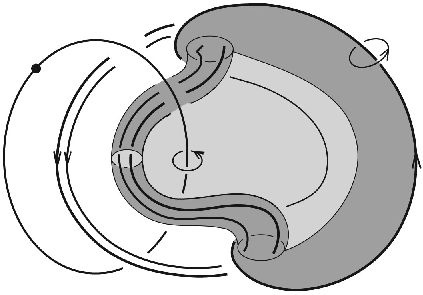
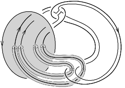
Consider the relative slice set-up in figure 3, where the dotted curves are defined in figure 2. To read off the word represented by $l_{1}$ in $M{\pi}_{1}(S^{3}\smallsetminus(l_{2}\cup l_{3}\cup l_{4}\cup r_{1}\cup r_{2}))$ it is useful to consider a $2$-stage capped grope [4] shown in figure 4, bounded by $l_{1}$: the two surface stages are embedded in the link complement while the caps intersect the link as shown in figure 4. (There are several versions of gropes considered in the literature. Throughout this section the term “grope” refers to half-gropes, see definition 2.4 and figure 2.1 in [2].)

A more detailed construction of this grope is shown in figure 5. Specifically, the link in figure 3 is a composition (in the sense of [2, Theorem 2.3]) of the two links shown in figure 5. Considering the standard genus one Heegaard decomposition of $S^{3}$, the components $l_{1},l_{2},r_{1}$ may be thought of as being contained in one of the solid tori, and the components $l_{3},l_{4},r_{2}$ are in the other solid torus of the decomposition. The first solid torus is pictured on the left in figure 5 as the complement of the dotted curve. The (genus one) first stage surface of the grope is shown in that figure. One cap for that surface intersects the components $l_{2},r_{1}$. There is another cap, intersecting the dotted curve, visible in the picture. The second stage is obtained by removing a small meridional disk from this cap. The resulting boundary component is then filled in by the genus two surface bounded by the curve $\Lambda$ in the complement of the link in figure 5 on the right.

The component $l_{1}$ is seen to be represented by the word

where $m_{i},a,b$ denote meridians to $l_{i}$, $r_{1}$, $r_{2}$ respectively. Recall that meridians are small circles linking the components, connected by arcs to the basepoint. The meridians, viewed as elements of the fundamental group of the link, depend on the choice of these arcs, as well as on the choice of the orientations of the small circles. It will be clear from the proof below that the choice of connecting arcs (and the choice of bands) is not going to be important for the argument since the difference between various choices is measured by higher order commutators which are trivial in the relevant Milnor group.

To fix the ambiguity with orientations, consider the orientations of the link components specified in figure 5 (also see figure 3). Orient the meridians using the “right-hand rule”, so the linking number of each component with its meridian is $+1$, as illustrated for $l_{1}$ in figure 5. A direct calculation shows that the exponents of all meridians in (3.4) are $+1$. It is worth mentioning that the techniques developed for the proof of theorem 1 in this paper, both for the Hopf link and for the Borromean rings, are quite robust. They work for a family of examples generalizing the main example in figure 2. For instance, the proof goes through if the band visible in the definition of the dotted curve in figure 2 were twisted. In this case the exponents of the two meridians labeled $b$ in (3.4) would have been opposite.

Consider band sums indicated in figure 3: the circled numbers are the indices of the slices (bounded by the curves $l_{i}$) that go over the $2$-handles attached to $r_{1}$, $r_{2}$. Specifically, add one parallel copy of $r_{1}$ to both $l_{3}$ and $l_{4}$, and add a parallel copy of $r_{2}$ with reversed orientation to $l_{2}$. Denote the components formed by the band summing by $l^{\prime}_{1},l^{\prime}_{2},l^{\prime}_{3},l^{\prime}_{4}$. ($l^{\prime}_{1}$ equals $l_{1}$ since no band-summing is performed on this component.)

Proof. A useful tool is the Half-grope lemma [2, Theorem 2.5] (also see [5, Theorem 2] for a streamlined proof). It states that if the components of an $n$-component link bound disjoint maps of $(n-1)$-stage gropes in $D^{4}$ then the link is homotopically trivial. Therefore in our context it suffices to find disjoint maps of three $2$-stage gropes into $D^{4}$, bounded by $l_{2}^{\prime},l_{3}^{\prime},l_{4}^{\prime}$. Consider two parallel copies of $r_{1}$ in figure 3 (without band-summing them with $l_{3},l_{4}$). Recall the detailed drawing of the handle diagram in the solid torus in figure 2. Since $l_{1}$ is missing from the link currently under consideration, observe that these two parallel copies of $r_{1}$ are isotopic within the solid torus to the curves labeled $\overline{3},\overline{4}$ in figure 6.

Consider the 7-component link in figure 6. The curve $l_{2}$ bounds an embedded $2$-stage grope, which can be easily located in the picture, in the complement of the other components in $S^{3}$. Extend these other 6 components by a product in the collar $S^{3}\times[0,\epsilon]$ in $D^{4}$. Since $l_{2}$ is not present in $S^{3}\times\{\epsilon\}$, the 6 components form the unlink and so bound disjoint disks in $S^{3}\times\{\epsilon\}$. Therefore the $7$ component link in figure 6 bounds disjoint $2$-stage gropes in $D^{4}$. (By definition the disk is an $n$-stage grope, for any $n$.) The link $(l^{\prime}_{2},l^{\prime}_{3},l^{\prime}_{4})$ is formed from the link in figure 6 by band-summing $l_{3}$ with the curve labeled $\overline{3}$, $l_{4}$ with $\overline{4}$, and also $l_{2}$ with $\overline{2}$ and $\overline{\overline{2}}$. Taking a boundary-connected sum of the $2$-stage gropes constructed above along the bands defining the band sums yields three disjoint $2$-stage gropes in $D^{4}$, bounded by $l^{\prime}_{2},l^{\prime}_{3},l^{\prime}_{4}$. The half-grope lemma completes the proof of proposition 3.2. ∎

Recall the commutator identities (cf. [8, Theorem 5.1])

We will now take a brief digression to discuss a basic fact, important for the argument here and in section 4, that conjugation in the commutator identities (3.5) and (3.7) below does not affect calculations in the Milnor group in our setting. The same comment applies to conjugation that results from different choices of basepoints. The key point is that the component $l_{1}$ is in the third term of the lower central series of ${\pi}_{1}(S^{3}\smallsetminus(l_{2}^{\prime}\cup l_{3}^{\prime}\cup l_{4}^{\prime}))$. Geometrically this is reflected in the fact that it bounds a two stage grope in figure 4; this may be seen algebraically using the expression (3.4) and the identities (3.5). Recall from section 3.1 that the Magnus expansion $M$ of the free Milnor group $M{\pi}_{1}(S^{3}\smallsetminus(l^{\prime}_{2}\cup l^{\prime}_{3}\cup l^{\prime}_{4}))$ into the ring $R_{x_{2},x_{3},x_{4}}$ is well-defined and injective. The Magnus expansion takes any element of the third term of the lower central series to a polynomial of the form $1+$(some linear combination of monomials of length $3$ in non-repeating variables $x_{2},x_{3},x_{4}$). The effect of conjugation on the Magnus expansion is the addition of higher order monomials. However since the monomials in the expansion $M(l_{1})$ are already of maximal length in $R_{x_{2},x_{3},x_{4}}$, any type of conjugation mentioned above does not change $M(l_{1})$. Since $M$ is injective, the element represented by $l_{1}$ in $M{\pi}_{1}(S^{3}\smallsetminus(l^{\prime}_{2}\cup l^{\prime}_{3}\cup l^{\prime}_{4}))$ is also unchanged by conjugation. An alternative argument for this fact, not using the Magnus expansion, may be given by directly using the defining Milnor relation (3.1).

The band summing (indicated in figure 3) defining the link $(l^{\prime}_{1},l^{\prime}_{2},l^{\prime}_{3},l^{\prime}_{4})$ results in substitutions $a=m_{3}m_{4}$ and $b=m_{2}^{-1}$ in (3.4). Disregarding conjugation in (3.5) and collecting commutators with distinct indices, one has

Using the identity $[x^{-1},y]=[y,x]^{x^{-1}}$ (where conjugation is again irrelevant), $l_{1}$ equals

Omitting conjugation in the Hall-Witt identity [8, Theorem 5.1]

one gets the Jacobi relation

establishing that $l_{1}=1\in MFree_{m_{2},m_{3},m_{4}}$.

Recall from proposition 3.2 that the link $(l^{\prime}_{2},l^{\prime}_{3},l^{\prime}_{4})$ is homotopically trivial. The point of the calculation above is that $l_{1}=1\in M{\pi}_{1}(S^{3}\smallsetminus(l^{\prime}_{2}\cup l^{\prime}_{3}\cup l^{\prime}_{4}))\cong MFree_{m_{2},m_{3},m_{4}}$. Therefore it follows from [9, Theorem 3] that $L^{\prime}=(l_{1},l^{\prime}_{2},l^{\prime}_{3},l^{\prime}_{4})$ is homotopically trivial and so its components bound disjoint maps of disks into $D^{4}$. This gives a solution up to link-homotopy to the relative-slice problem for the Hopf link which is “standard” in the sense of remark 3.1.

The detail that is missing from the conclusion of the proof of theorem 1 for the Hopf link is that the two copies of the manifold $M$ have to be embedded, while the outcome of the argument so far is a map of two copies $A_{1},A_{2}$ of $A$ into $D^{4}$ where individual $2$-handles have self-plumbings. (Moreover, as discussed in the introduction the embeddings are required to be isotopic to the original embedding $M\subset D^{4}$.) The null-homotopies produced as a result of Milnor group calculations may be realized as a sequence of standard “elementary homotopies” of link components. The manifold $M$ will be defined to be $A$ with a number of self-plumbings of its two $2$-handles, determined by those of both $A_{1}$ and $A_{2}$.

The precise details of the construction of $M$ are as follows. It is worth mentioning right away that the standard condition is imposed on each individual embedding of $M$. That is, after $M$ is constructed two copies of it will be disjointly embedded with their attaching circles corresponding to the two components of the Hopf link, and the embedding of each copy will be shown to be standard after the other component is disregarded. Figure 7 is a concise illustration of the construction.

Each of the two links $(l_{1},l_{2},r_{2})$ and $(l_{3},l_{4},r_{1})$ is a three-component unlink, and band sums in the proof above may be easily found so that both $(l^{\prime}_{1},l^{\prime}_{2})$, $(l^{\prime}_{3},l^{\prime}_{4})$ are two-component unlinks. Taking a band sum of $l_{2}$ with $r_{2}$ and capping off with the core of the $2$-handle attached to $r_{2}$ amounts to a $(1,2)$-pair of critical points of the slice for $l_{2}$ with respect to the radial Morse function on $D^{4}$. (This Morse function is considered on the original $4$-ball which contains the $2$-handles attached along $r_{1},r_{2}$ and into which the manifolds $A_{1},A_{2}$ are embedded, see the second paragraph of section 3.2. The slightly smaller $4$-ball where the relative-slice problem is being considered is obtained by removing the collars on the attaching regions of $A_{1},A_{2}$.) Since $(l_{1},l_{2},r_{2})$ is the unlink, this pair of critical points can be canceled and (ignoring the components $l_{3},l_{4}$) the result is an isotopy of $(l_{1},l_{2})$ in $S^{3}\times I$. (Compare with figure 15 in [6].) Similarly, (considering just the last two components) band summing $l_{3}$ and $l_{4}$ with copies of $r_{1}$ may be realized instead as an isotopy of $l_{3},l_{4}$.

We summarize the set-up: the $4$-component link $L^{\prime}:=(l^{\prime}_{1},\ldots,l^{\prime}_{4})$ is null-homotopic, and the two component sub-links $(l^{\prime}_{1},l^{\prime}_{2}),(l^{\prime}_{3},l^{\prime}_{4})$ are individually unlinks. We will next construct specific null-homotopies of the components of $L^{\prime}$. Start with any link homotopy from $L^{\prime}$ to the $4$-component unlink. Rather than capping them off by disks right away, let the first two components move by an isotopy away from the last two components. For reasons which will be clear below, next we run the entire link-homotopy of $l^{\prime}_{3},l^{\prime}_{4}$ backwards, while the first two components stay fixed as unknots away from $l^{\prime}_{3},l^{\prime}_{4}$. The result is a $4$-component unlink which may be capped off by disks. Denote the resulting link homotopies (disjoint annuli with self-intersections) of $l^{\prime}_{1},l^{\prime}_{2}$ by $H$ and $l^{\prime}_{3},l^{\prime}_{4}$ by $H^{\prime}$, see the diagram on the left in figure 7. To prepare for the following step of the construction, note that both $H,H^{\prime}$ are level-preserving singular maps $(S^{1}\sqcup S^{1})\times[0,1]\longrightarrow S^{3}\times[0,1]$ giving two-component unlinks at times $0,1$. Their singularities consist of finitely many double point self-intersections, and they are isotopies when restricted to sub-intervals of $[0,1]$ not containing singular points. Although $H^{\prime}$ is defined using $l^{\prime}_{3},l^{\prime}_{4}$, it can be “applied” to any two-component unlink in $S^{3}\times\{0\}$, for example to $l^{\prime}_{1},l^{\prime}_{2}$.

The result so far is insufficient for the definition of $M$ since $H,H^{\prime}$ may be non-isotopic in $D^{4}$. A suitable link-homotopy of $L^{\prime}$ is constructed instead as follows. As shown on the right in figure 7, as a preliminary step start by applying the link homotopy $H^{\prime}$ to the components $l^{\prime}_{1},l^{\prime}_{2}$, while letting $l^{\prime}_{3},l^{\prime}_{4}$ move by an isotopy in their complement. More precisely, recall from the previous paragraph that $H^{\prime}$ is a level-preserving map $(S^{1}\sqcup S^{1})\times I\longrightarrow S^{3}\times I$ which is an isotopy at generic times and whose singularities consist of double point self-intersections at finitely many times. Given two components, $l^{\prime}_{3}$ and $l^{\prime}_{4}$, in the complement of $l^{\prime}_{1},l^{\prime}_{2}$ in $S^{3}\times\{0\}$ there exists an isotopy moving them in the complement of $H^{\prime}$: a level-preserving embedding $(S^{1}\sqcup S^{1})\times I\hookrightarrow S^{3}\times I\smallsetminus\,{\rm image}(H^{\prime})$. Indeed, each double point of $H^{\prime}$ is described by a movie where two strands of either $l^{\prime}_{1}$ or $l^{\prime}_{2}$ move by an isotopy in $S^{3}$ and intersect in a single point. By general position, since $l^{\prime}_{3},l^{\prime}_{4}$ are $1$-dimensional submanifolds of $S^{3}$, they may be kept disjoint from $H^{\prime}$ during this movie. This completes the argument for the existence of an isotopy of $l^{\prime}_{3},l^{\prime}_{4}$ in the complement of $H^{\prime}$.

Since $H^{\prime}$ was constructed as a link-homotopy followed by its reverse, the outcome of the previous paragraph is an identical copy of $L^{\prime}=(l^{\prime}_{1},\ldots,l^{\prime}_{4})$. Now run the link-homotopy $H,H^{\prime}$ of $L^{\prime}$. The result is a $4$-component unlink. Cap off the first two components with disks and apply $H$ to the $3$-rd and $4$-th components. Finally, cap off the last two components. Now the null-homotopy of $(l^{\prime}_{1},l^{\prime}_{2})$ is isotopic to the null-homotopy of $(l^{\prime}_{3},l^{\prime}_{4})$: up to isotopy each one is $H^{\prime}$ followed by $H$ and then capped off with standard disks, figure 7. Define $M$ to be either of the two embeddings of the manifold $A$ in figure 2 with self-plumbings of the $2$-handles constructed above. This yields an embedding of two standard copies of $M$ as required in the part of theorem 1 concerning the Hopf link.

Consider the complement of the manifold $A$ in figure 2, $B=D^{4}\smallsetminus A$. A handle decomposition for $B$ (with the attaching curve $\beta$) may be obtained from that of $A$ by exchanging the $1$- and $2$-handles as explained in [2], see figure 10. The question relevant from the perspective of the A-B slice problem is whether the Borromean rings bound disjoint embeddings of three copies of $A$, and also disjoint embeddings of three copies of $B$ where the embeddings are all standard, see remark 3.1. (The origin of the “standard” condition on embeddings is in the formulation of the A-B slice problem [1, 2]: it reflects the covering group action on the $4$-ball, which is predicted by the $4$-dimensional topological surgery conjecture.)

It was proved in section 4 that there are no disjoint embeddings of three copies of $A$. We will next examine the embedding problem for three copies of $B$ with the boundary condition given by the Borromean rings. It is worth noting that the Hopf link is not $B$-slice. Observe in figure 10 that the attaching curve $\beta$ bounds a surface in $B$. Therefore the non-triviality of the linking number of the Hopf link implies that its components do not bound disjoint copies of $B$. In fact, this argument immediately generalizes to show that the Hopf link is not $A$-$B$ slice: the attaching curve of one of the two sides of any decomposition $D^{4}=A\cup B$ bounds rationally. Therefore the linking number is an obstruction. The interested reader will find related in-depth discussion in [3].

As in section 4 the embedding question for the Borromean rings is reformulated as a relative-slice problem, shown in figure 11. The problem is to find disjoint disks (possibly with self-intersections) for the link components labeled $1$-$6$ in the handlebody $D^{4}\cup$ six zero-framed $2$-handles attached along the dotted curves. The sought solution has to satisfy the standard assumption discussed in remark 3.1. This means that the slices for $l_{1},l_{4}$ are not allowed to go over the two $2$-handles attached to the dotted curve on the upper left, and similarly $l_{2},l_{5}$ should not go over the two $2$-handles on the right, and $l_{3},l_{6}$ should not go over the $2$-handles on the lower left.

The circled indices next to the dotted component in figure 11 indicate band-sums such that all $\bar{\mu}$-invariants of the resulting link of length $\leq 3$ vanish. The original obstruction for the Borromean rings, $\bar{\mu}_{123}$, is of length 3, so the “primary” obstruction is killed. To find a link-homotopy solution to this relative slice problem one needs all $\bar{\mu}$-invariants up to order 6 to be zero. Unlike the settings in sections 3, 4, conjugation corresponding to the choice of meridians and bands is important here. It seems likely that a careful choice of bands should give rise to a link homotopy solution, but at present this is an open question.

Consider the submanifolds $A^{\prime},A^{\prime\prime}\subset D^{4}$ shown in figure 12, closely related to the submanifold $A$ constructed in section 2, and consider the corresponding decompositions $D^{4}=A^{\prime}\cup B^{\prime}$, $D^{4}=A^{\prime\prime}\cup B^{\prime\prime}$.

A solution up to link-homotopy to the relative-slice problem for three copies of $A^{\prime\prime}$ on the Borromean rings is given in figure 13. (Note the assymetry of labels going over the top two components: some assymetry is necessary since a solution does not exist for three copies of $A$, according to theorem 1.) The reader is encouraged to check that the resulting product of commutators representing $l_{6}$ in non-repeating variables indeed equals the element $w$ from lemma 4.3! It is not difficult to check using $\bar{\mu}_{123}$ that the Borromean rings do not support standard embeddings of three copies of the other side of this decomposition, $B^{\prime\prime}$.

The decomposition $D^{4}=A^{\prime}\cup B^{\prime}$ was the subject of the papers [6, 7]. It is shown in [7] that the Borromean rings do not bound three standard copies of $A^{\prime}$.

Given a decomposition of the $4$-ball, $D^{4}=A\cup B$, into two codimension zero submanifolds where the “attaching curves” ${\alpha},{\beta}$ of $A,B$ form the Hopf link in $S^{3}=\partial D^{4}$, an important question in the A-B slice program is to determine whether there is necessarily an obstruction to the Borromean rings being both $A$-slice and $B$-slice in the sense of theorem 1. The side which carries an obstruction (if there is one) is called “strong”, see [2] and also [6, 7]. The goal is to determine a strong side for any decomposition $D^{4}=A\cup B$.

To summarize the results of this paper in the context of the AB slice problem, in each of the examples considered here, $D^{4}=A\cup B=A^{\prime}\cup B^{\prime}=A^{\prime\prime}\cup B^{\prime\prime}$ (figures 2, 12), one of the two sides is found to be “strong”. A novel type of an obstruction is used here: the key to deciding which side is strong is whether the element $w$ in lemma 4.3 is in the image of the relator curves on the relevant (in our notation, $A$)-side. The work presented here admits an immediate generalization giving rise to an obstruction for an infinite family of decompositions by further Bing doubling the links describing the Kirby diagrams in figures 2, 12.

To provide a verification that the element $w$ in lemma 4.3 is in the subspace $J\subset V$, in other words that $w$ is trivial modulo the Jacobi and antisymmetry relations, listed below is an expression of each commutator in the definition of $w$ as a linear combination of the commutators forming the basis of $V/J$ in proposition 4.4. This list also makes it clear that the dimension of $U\cap J$ in the statement of lemma 4.3 is precisely $1$ (and not greater).

References

- [1] M. Freedman, A geometric reformulation of four dimensional surgery, Topology Appl., 24 (1986), 133-141.
- [2] M. Freedman and X.S. Lin, On the -slice problem, Topology Vol. 28 (1989), 91-110.
- [3] M. Freedman and V. Krushkal, Topological arbiters, J. Topol. 5 (2012), 226-247.
- [4] M. Freedman and F. Quinn, The topology of 4-manifolds, Princeton Math. Series 39, Princeton, NJ, 1990.
- [5] V. Krushkal, Exponential separation in -manifolds, Geom. Topol. 4 (2000), 397-405.
- [6] V. Krushkal, A counterexample to the strong version of Freedman’s conjecture, Ann. of Math. 168 (2008), 675-693.
- [7] V. Krushkal, Robust four-manifolds and robust embeddings, Pacific J. Math. 248 (2010), 191-202.
- [8] W. Magnus, A. Karrass and D. Solitar, Combinatorial group theory: Presentations of groups in terms of generators and relations, Interscience Publishers, New York-London-Sydney 1966.
- [9] J. Milnor, Link Groups, Ann. Math 59 (1954), 177-195.
- [10] C. Reutenauer, Free Lie algebras, London Mathematical Society Monographs, Oxford University Press, New York, 1993.