Constraining Modified Chaplygin Gas Parameters
D. Panigrahi¹¹ 1 Sree Chaitanya College, Habra 743268, India and also Relativity and Cosmology Research Centre, Jadavpur University, Kolkata - 700032, India, e-mail: dibyendupanigrahi@yahoo.co.in, B. C. Paul²² 2 Department of Physics, University of North Bengal, Dist. - Darjeeling, PIN- 734013, India, e-mail : bcpaul@iucaa.ernet.in and S. Chatterjee³³ 3 IGNOU Convergence Centre, New Alipore College, Kolkata - 700053, India and also Relativity and Cosmology Research Centre, Jadavpur University, Kolkata - 700032,India e-mail : chat_ sujit1@yahoo.com

Following the high redshift supernovae data in the last decade [1] we know that when interpreted within the framework of the standard FRW type of universe (homogeneous and isotropic) we are left with the only alternative that the universe is now passing through an accelerated phase of expansion with baryonic matter contributing only four percent of the total energy budget. Observational results coming from CMBR studies  [2] also point to this conclusion engaging a large community of cosmologists  [3] and references therein) to embark on a quest to explain the cause of the acceleration. The teething problem now confronting researchers is the identification of the mechanism that triggered the late inflation. Researchers are mainly divided into two groups � either suggesting a modification of the original general theory of relativity or invoking any mysterious fluid in the form of an evolving cosmological constant or a quintessential type of scalar field. But as debated at length in the literature both the alternatives face serious problems mainly at the theoretical and conceptual level. Typically, the late acceleration has been attributed to a mysterious dark energy (DE) which contributes about three fourth of the cosmic substratum. Another unknown matter component of the universe is the dark matter (DM), the missing mass necessary to hold together the galaxy clusters and also needed to explain the current large scale structure of the universe.

In the literature a good number of dark energy models are proposed but little is precisely known about it. Nowadays, the dark energy problem remains one of the major unsolved problems of theoretical physics [4]. On the way of searching for possible solutions of this problem various models are explored during last few decades referring to e.g. new exotic forms of matter (e.g. quintessenceï)  [5], phantom  [6], holographic models  [7], string theory landscape [8] Born-Infeld quantum condensate  [9], modified gravity approaches [10], inhomogeneous spacetime [11] etc  (readers interested in more detail for a comprehensive overview of existing theoretical models may refer to [12])

Even though the cosmological constant allows for the cosmic acceleration at late times, the observational bounds on $\Lambda$ are incompatible with theoretical predictions of a gravitational vacuum state. Grosso modo, the $\Lambda$ model does well in fitting most observational data but the density parameter corresponding to $\Lambda$ and matter are of the same order of magnitude, surprisingly close to each other, even though $\Lambda$ is a constant during the entire evolutionary history of the universe. These two thorny shortcomings, namely the fine tuning and the coincidence problems, disturb the otherwise appealing picture of a cosmological constant and dramatically plague the so called $\Lambda$CDM model. To circumvent this difficulty and host others people invoke a variable $\Lambda$ model but that too is beset with serious field theoretic problems  [13]. Another possibility to obtain accelerated expansion is provided by theories with large extra dimensions known as braneworlds  [14] but one has to hypothesize the existence of extra spatial dimensions in these models.

Among the different theories put forward in the literature in recent times, the single component fluid known as Chaplygin gas(CG) with an equation of state (EoS) $p=-\frac{B}{\rho}$  [15], where $\rho$ and $p$ are the energy density and pressure respectively and $B$ is a constant has attracted large interest in cosmology. Although the model is very successful in explaining the SNe Ia data it shows that CG does not pass the tests connected with structure formation and observed strong oscillations of matter power spectrum  [16]. One can circumvent this situation in the generalised chaplygin gas(GCG) proposed with $p=-\frac{B}{\rho^{\alpha}}$ with $\alpha$, constrained in the range $0<\alpha<1$. Since the inferences from the $\Lambda CDM$ and GCG models are almost similar, atleast from the observational fallouts this model is further modified either considering $B$ as a function of the redshift($z$) as $B=B(z)$  [17] or assuming an EoS as,

$$p=A\rho-\frac{B}{\rho^{\alpha}}$$

(1)

(MCG) [18], where $A$ is a new constant parameter of the theory. Thus MCG may be looked upon as a mixture of a barotropic perfect fluid and GCG. Although it suffers from serious shortcomings e.g., it violates the time honoured principle of energy conditions, still its theoretical conclusions are found to be in broad agreement with the observational results coming out of gravitational lensing or recent CMBR and SNe data in varied cosmic probes. This is generally achieved through a careful maneuvering of the value of the newly introduced arbitrary constant. The viability of the scenario has been tested by a number of cosmological probes, including SNe Ia data [19], lensing statistics [20], age-reshift tests [21], CMB measurements [22], measurements of X Ray luminosity of galaxy clusters [23], statefinder parameters [24]. Another interesting feature of the MCG is that it can show radiation era in the early universe. At late times MCG behaves as a cosmological constant and can be fitted to $\Lambda CDM$.

Furthermore, dark matter (in short, DM) and dark energy (DE) are considered as different manifestations of the same component and describes the dark sector as some kind of fluid whose physical properties depend on the scale: it behaves as DM at high densities and transforms into DE at lower ones. Most of these United Dark Matter models invoke the generalized Chaplygin gas (GCG), a perfect fluid characterized by a negative pressure which is inversely proportional to the energy density.

Using modified chaplygin gas (in short, MCG) in FRW universe a number of cosmological models have been discussed in the literature. In most of the models the values of the so called free parameters are picked up by hand in order to suit the best fit values with the observational results without much physical considerations. It is important to study cosmological models from observational contexts which naturally impose a constraint on the values of the free parameters. In view of the above considerations, in this work we determine the constraints on the free parameters of the model by drawing the usual contour plot diagrams. However two works in this field are worth mentioning. In an earlier one Jianbo Lu et al [25]have apparently come to the conclusion via usual contour plot diagram that the recently observed data give credence to both the MCG as well as other fashionable models so that it is very difficult to choose one over the other. This is in line with earlier results in this field [26]. Secondly in a very recent communication Wang et al [27] have also studied in depth the constraints on $\alpha$ in GCG formalism in two distinct cases - one pertaining to a barotropic equation of state and the other to a dark matter with some specific properties. In what follows we have discussed and compared, in brief, our own findings in this field vis-a-vis Wang et al’s work at the end of our paper in sec. 5. Our work is primarily focussed on two domains. First to study the dynamics of FRW cosmological scenario with MCG as matter field as also to obtain constraints on the so called three free parameters with the help of contour diagram to achieve the best fit with current observational findings. The paper is organised as follows: in sec. 2 we build up the evolution equations, while the nature of evolution and analysis of instability of our model are dealt with in some detail in sec. 3. In sec. 4 we discuss the observational data, namely Stern data, measurement of baryon acoustic oscillations (BAO) peak parameters and CMB shift data to draw contour diagram for the permissible range of values of the pair of parameters ($\alpha,A$),($\omega_{ode},A$) and ($\Omega_{odm},A$). Finally in sec. 5 we give a brief discussion.

We consider a flat spherically symmetric homogeneous spacetime with line element

$$ds^{2}=dt^{2}-a^{2}(t)~(dr^{2}+r^{2}d\Omega^{2})$$

(2)

where the scale factor, $a(t)$ depends on time only. Taking a comoving coordinate system such that $u^{0}=1,u^{i}=0~(i=1,2,3)$ and $g^{\mu\nu}u_{\mu}u_{\nu}=1$ where $u_{\mu}$ represents the 4- velocity, the energy momentum tensor for a perfect fluid distribution in the above defined coordinates is given by

$$T^{\mu}_{\nu}=(\rho+p)\delta_{0}^{\mu}\delta_{\nu}^{0}-p\delta_{\nu}^{\mu}$$

(3)

where $\rho(t)$ is the matter density and $p(t)$ the isotropic pressure. The Einstein field equations for the above metric are given by

	$\displaystyle 3H^{2}$	$\displaystyle=$	$\displaystyle\rho$		(4)
	$\displaystyle 2\dot{H}+3H^{2}$	$\displaystyle=$	$\displaystyle-p$		(5)

where $H(=\frac{\dot{a}}{a})$ represents the Hubble parameter and we use units where 8 $\pi\;G$ = 1. The conservation equations for matter fields are given by

$$\nabla_{\nu}T^{\mu\nu}=0$$

(6)

which in turn yields

$$\dot{\rho}_{total}+3H(\rho_{total}+p_{total})=0$$

(7)

We now consider a mixture of fluids, where baryons represents one of the component and conservation of baryons leads to the continuity equation that can be separated into two equations, given by

	$\displaystyle\dot{\rho}_{b}+3H(\rho_{b}+p_{b})=0$		(8)
	$\displaystyle\dot{\rho}+3H(\rho+p)=0$		(9)

where $\rho_{total}=\rho+\rho_{b}$ and the subscript $b$ denotes the baryons. The component of other part is a mixture of dark matter and dark energy. In our model we consider Modified Chaplygin gas (MCG) as one of the candidate for dark energy and consequently the mathematical expressions are given by $p=p_{de}$ and $\rho=\rho_{de}+\rho_{dm}$, which obeys an EoS given by equation (1). In the above, the subscripts $dm$ and $de$ denote dark matter and dark energy respectively. Let $p_{de}=\omega_{de}\rho_{de}$, where the EoS parameter for dark energy is $\omega_{de}$. Using eq. (1) in conservation equation given by eq. (9), one obtains an energy density given by

$$\rho=\left[\frac{B}{1+A}+c(1+z)^{3(1+\alpha)(1+A)}\right]^{\frac{1}{1+\alpha}}$$

(10)

where $c$ is an integration constant. From eq. (10) it is evident that $A\neq-1$ is required for a finite $\rho$ .

The energy densities of the dark energy and the dark matter are now determined using the set of dynamical equations given in the sec. 2 such that

$\displaystyle\rho_{de}=\frac{A\left[\frac{B}{1+A}+c(1+z)^{3(1+\alpha)(1+A)}\right]-B}{\omega_{de}\left[\frac{B}{1+A}+c(1+z)^{3(1+\alpha)(1+A)}\right]^{\frac{\alpha}{1+\alpha}}},$

(11)

$\displaystyle\rho_{dm}=\rho-\rho_{de}=\frac{\left(\omega_{de}-A\right)\left[\frac{B}{1+A}+c(1+z)^{3(1+\alpha)(1+A)}\right]+B}{\left[\frac{B}{1+A}+c(1+z)^{3(1+\alpha)(1+A)}\right]^{\frac{\alpha}{1+\alpha}}}.\hskip 51.21504pt$

(12)

Now the constants $B$ and $c$ can be expressed as,

$$B=\left\{A(1-\Omega_{ob})-\omega_{ode}\Omega_{ode}\right\}(1-\Omega_{ob})^{\alpha}\rho_{oc}^{(1+\alpha)}$$

(13)

$$c=(1-\Omega_{ob}+\omega_{ode}\Omega_{ode})\frac{(1-\Omega_{ob})^{\alpha}}{1+A}\rho_{oc}^{(1+\alpha)}$$

(14)

where $\rho_{oc}$ represents critical density, and label $o$ denotes quantities that estimate present values.

In the case of GCG, $B$ is one free parameter but in the Modified Chaplygin gas (MCG) the parameter $B$ is related to $A$ and the present value of the density parameter, $\alpha$ and the EoS parameter via equation (13) so that when we constrain $A$ from the observational inputs the other constant $B$ is automatically fixed up. Further from the equation (10) we find that $B$ is important when $z$ is very small and the universe is dark energy dominated. So knowing the dark energy contribution $B$ can be fixed, which, however, is not considered in the present work.

The energy density of the universe can be expressed in terms of redshift parameter, $z$ which is given by

$$\rho(z)=\frac{(1-\Omega_{ob})^{\frac{\alpha}{1+\alpha}}}{(1+A)^{\frac{1}{1+\alpha}}}\biggl[A(1-\Omega_{ob})-\omega_{ode}\Omega_{ode}\\ +(1-\Omega_{ob}+\omega_{ode}\Omega_{ode})(1+z)^{3(1+\alpha)(1+A)}\biggr]^{\frac{1}{1+\alpha}}$$

(15)

where we use $a(t)=\frac{1}{1+z}$.

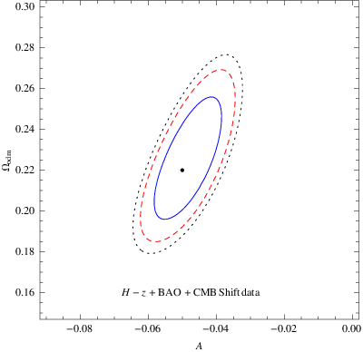
We consider four values of $A$ & $\alpha$ as permitted by the contours drawn in figs. (1) & (2), the density variation with $z$ are plotted and found that the universe is denser for $A=-0.1072$ and $\alpha=1.376$. Other permitted values of $A$ and $\alpha$ are $(-0.05,0.50);(0.002,0.100);(0.0446,-0.0583)$ respectively. However, from fig. (3) it is clear that the range of $A$ is further restricted to ($-0.0649$ to $-0.0319$) at $95.4\%$ confidence level. This implies that the dark matter parameter dictates that $A$ should be slightly less than zero. The prediction in our model agrees with that obtained by Fabris et al [28]. Using the WMAP predicted values [2] namely, the current density parameters $\Omega_{ode}=0.734\pm 0.029$, $\Omega_{odm}=0.222\pm 0.026$ and $\Omega_{ob}=0.0449\pm 0.0028$, we explore the variation of the density of the universe $\rho(z)$ with redshift $z$. The variation of $\rho(z)$ with $z$ is plotted in fig. (4) for different $A$ and $\alpha$ values. As expected the density of the universe increases with an increase in $z$ values, as more the value of $z$ more the observations probe the early universe. It is also noted that as one picks up more and more negative values of $A$ with positive $\alpha$, it leads to greater energy density in the early universe for a fixed $z$ value. The permitted range of values of $A$ and $\alpha$ will be discussed in sec. 4, the present energy density of the universe is independent of $A$ & $\alpha$ at $z=0$ and attains a value $(\rho)_{z=0}=(1-\Omega_{ob})$ which also follows from the eq.(15). The study reveals the dynamical property of the universe which shows how fast the universe is accelerating for different values of $A$ & $\alpha$.

Using eqs. (1), (10), (13) and (14), we obtain the equation of state parameter for the MCG model given by

$$\omega(z)=\frac{p}{\rho}=-\frac{A(1-\Omega_{ob})-\omega_{ode}\Omega_{ode}-A(1-\Omega_{ob}+\omega_{ode}\Omega_{ode})(1+z)^{3(1+\alpha)(1+A)}}{A(1-\Omega_{ob})-\omega_{ode}\Omega_{ode}+(1-\Omega_{ob}+\omega_{ode}\Omega_{ode})(1+z)^{3(1+\alpha)(1+A)}}$$

(16)

For consistency check we note that with $B=0$ eq. (13) gives $A=\frac{\omega_{0de}\Omega_{ode}}{1-\Omega_{ob}}$ leading to a barotropic equation of state parameter $\omega(z)=A$, which is negative as $\omega_{ode}$ is negative definite. In our case an accelerating universe is permitted with $A<-\frac{1}{3}$. Considering $\omega_{ode}=-1.05$, $\Omega_{ode}=0.734$, $\Omega_{odm}=0.222$ and $\Omega_{ob}=0.044$, we get $A\approx-0.80$ for a viable cosmology. This model is in agreement with $\Lambda$CDM model. For $A=0$, this MCG model reduces to GCG model. In this case

$$\omega(z)=\frac{\omega_{ode}\Omega_{ode}}{-\omega_{ode}\Omega_{ode}+\left(1-\Omega_{ob}+\omega_{ode}\Omega_{ode}\right)(1+z)^{3(1+\alpha)}}$$

(17)

It is noted from the contour drawn in fig. (2) that $\omega_{ode}$ lies between $-1.194$ to $-0.8771$ at $95.4\%$ confidence limit. It is also noted that the function $\omega(z)$ is always negative for entire range of values of $\omega_{ode}$ with (i) $A=-0.05$ & $\alpha=0.50$, (ii) $A=-0.1072$ & $\alpha=1.376$ and (iii) $A=0.002$ & $\alpha=0.100$. However, we note that $\omega(z)$ is negative at the present epoch which was positive in the early epoch for $A=0.0446$ and $\alpha=-0.0583$ . Thus a transition to an accelerating universe is permitted.

In fig. (1), we plot variation of $A$ with $\alpha$. It is evident that it admits $A=0$, $\alpha=0.10$. At $z=0$, $\omega(z)$ becomes negative for negative values of $\omega_{ode}$, admitting an accelerating universe. The evolution of $\omega(z)$ with $z$ is shown in the fig. (5). It is evident that $\omega(z)$ is mostly flat in the high redshift region ($z>2.0$) which is very steep at low redshift ($z$) region. We note that $\omega(z)$ is always negative as one extrapolates from past to future for the values of $A=-0.1072$ & $\alpha=1.376$ , $A=-0.05$ & $\alpha=0.50$ and $A=0.002$ & $\alpha=0.100$, but for $A=0.0446$ & $\alpha=-0.0583$, it is positive in the past (shown with $z\approx 3.80$). In this case we get $\omega(z)=0$ at $z\approx 3.80$, corresponding to a dust dominated universe in the recent past. Again it is found that at $z=0$, $\omega(z)$ attains $-0.80$ which is independent of $A$ & $\alpha$. It also follows from the eq. (16) that $\omega(z)|_{z=0}=\frac{\omega_{ode}\Omega_{ode}}{1-\Omega_{ob}}$.

In the context of the theory of linear perturbation the squared speed of sound, $v_{s}^{2}$, plays a very important role in determining the stability or instability of a given perturbed state. The positive sign indicates the periodic propagating mode for a density perturbation and the system points to stability for a given mode. The negative sign (imaginary value of speed) shows an exponentially growing mode for a density perturbation indicating the instability of a given mode. Generally the evolution of sound speed in the linear regime of perturbation is independent of the dynamics of the background cosmology as follows:

$$v_{s}^{2}=\frac{dp}{d\rho}=\frac{1}{3H}\frac{d}{dH}\left[H^{2}\left(q-\frac{1}{2}\right)\right]$$

(18)

Thus the sign of $q$ determines the sign of $v_{s}^{2}$ via the transition epoch from the CDM dominated phase to DE dominated phase. From the above description one can easily find that the growth of perturbation is dependent on the choice of DE model of background dynamics. For the Chaplygin gas (CG) model we have

$$v_{s}^{2}=-\frac{B}{\rho^{2}}=-\omega(z)$$

(19)

If we further take the CG as a quintessence DE model with $-1<\omega(z)<0$, the squared speed is always positive. So the stability of the CG model against density perturbation at any cosmic scale factor is guaranteed.
In the case of GCG model the situation is almost similar. We see

$$v_{s}^{2}=-\alpha\omega(z)$$

(20)

Once again in the quintessence range the GCG model is instable against density perturbation if $\alpha<0$ and stable if $\alpha>0$. From the observational data we know that $\alpha$ is always positive and this ensures the stability of the model. For the MCG model under consideration the situation is, however more involved. We get for quintessence zone

$$v_{s}^{2}=A(1+\alpha)-\alpha\omega(z)$$

(21)

Thus for $A\geq 0$ the system is always stable. But for negative $A$ the stability depends on the relative magnitudes of $\omega(z)$, $A$ and $\alpha$.

Now eq.,(16) and(21) further give for our case under consideration

$\displaystyle v_{s}^{2}=A(1+\alpha)+\alpha\left[\frac{A(1-\Omega_{ob})-\omega_{ode}\Omega_{ode}-A(1-\Omega_{ob}+\omega_{ode}\Omega_{ode})(1+z)^{3(1+\alpha)(1+A)}}{A(1-\Omega_{ob})-\omega_{ode}\Omega_{ode}+(1-\Omega_{ob}+\omega_{ode}\Omega_{ode})(1+z)^{3(1+\alpha)(1+A)}}\right]$

(22)

In fig.(6) we plot the variation of the squared speed of sound $v^{2}_{s}$ with redshift parameter $z$. It is observed that the speed of sound $v_{s}$ is positive definite for $A=-0.1072$ & $\alpha=1.376$ and $A=-0.05$ & $\alpha=0.50$ (i.e., negative values of $A$) for low value of $z$, which, however, becomes $v_{s}^{2}<0$ for high redshift region. This leads to instability of the MCG fluids as noted by Mei Deng  [29]. It is argued that for $\alpha>-1$, $(v_{s}^{2})_{z\rightarrow\infty}\approx 0$. However, we note that instability sets in our case with $\alpha\geq-0.0583$ leading to $v_{s}^{2}=0$ for finite $z$ accommodating the results obtained by Mei Deng.

We note that the squared speed of sound does not exceed that of light for $A=-0.1072$ & $\alpha=1.376$ at $z=0$. However, in future, i.e., ($1+z<1$) it is possible, $v_{s}$ exceeds the speed of light for the above value of $A$ and $\alpha$. This results in a perturbation of the spacetime and a perturbative analysis of the whole system shows that it favours structure formation [30]. For $A=0.0446$ & $\alpha=-0.0583$, the MCG fluids are unstable for lower $z$ value. However for high redshift, i.e., in the early universe $v_{s}^{2}>0$ is permitted. It is very interesting to note that for $A=0.002$ & $\alpha=0.100$, $v_{s}^{2}$ is always positive. At high redshift region it was lower than present epoch. Again in future $v_{s}^{2}$ will be higher but does not exceed the velocity of light. At $A=0$, $v_{s}^{2}=-\alpha\omega(z)$ and $\omega(z)<0$ in this case, which gives positive value of $v_{s}$(since $\alpha$ is slightly greater than zero at $A=0$). From eq. (22) it follows that the present value of $v_{s}^{2}$ is $(v_{s}^{2})_{z=0}=A(1+\alpha)-\frac{\alpha\omega_{ode}\Omega_{ode}}{1-\Omega_{ob}}$ obtained by putting $z=0$. The squared speed of sound $v_{s}^{2}$ depends both on $A$ and $\alpha$ at low redshift $z=0$. This is unlike the cases of $\rho$ and $\omega(z)$.

It is evident from fig-6 that at high redshift region ( $1+z<1.7$ ) $v_{s}^{2}<0$ for $A=-0.05,\alpha=0.50$ and $A=-0.1072,\alpha=1.376$. This leads to instability of the MCG fluid at high $z$, i.e., at early universe, which helps in structure formation. But the model is stable at the present epoch (i.e., $z=0$) and also $0<v_{s}^{2}<c_{s}^{2}$.

Now, we consider a spatially flat FRW universe with background fluid described by an exotic fluid component namely, MCG and baryon component. From the dynamical field equations we obtain dimensionless Hubble parameter

$$E^{2}(z)\equiv\frac{H^{2}}{H_{o}^{2}}=\frac{(1-\Omega_{ob})^{\frac{\alpha}{1+\alpha}}}{(1+A)^{{}^{\frac{\alpha}{1+\alpha}}}}\biggl[A\left(\Omega_{ode}+\Omega_{odm}\right)-\omega_{ode}\Omega_{ode}\\ +\Omega_{odm}(1+z)^{3(1+\alpha)(1+A)}+\Omega_{ode}(1+\omega_{ode})(1+z)^{3(1+\alpha)(1+A)}\biggr]^{\frac{1}{1+\alpha}}+\Omega_{ob}(1+z)^{3}$$

(23)

The variation of normalized Hubble parameter with redshift is shown in the fig. (7). It is observed that normalised Hubble parameter changes more sharply with $z$ for the set ($A=-0.1072$, $\alpha=1.376$) compared to other sets, where $A$ is less negative in line with the fact that more negative $A$ values imply a more accelerating model. It attains $E^{2}(z)=1$ at the present epoch $z=0$.

Using the above equations, the densities of different components of the energy namely, $\Omega_{dm}$, $\Omega_{de}$ and $\Omega_{b}$ are obtained which are given below :

$$\Omega_{de}=\frac{(1-\Omega_{ob})^{\frac{\alpha}{1+\alpha}}(1+A)^{\frac{\alpha}{1+\alpha}}}{\omega_{de}E^{2}(z)}\biggl[\frac{A}{1+A}\biggl\{A(1-\Omega_{ob})-\omega_{ode}\Omega_{ode}\\ +(1-\Omega_{ob}+\omega_{ode}\Omega_{ode})(1+z)^{3(1+\alpha)(1+A)}\biggr\}^{\frac{1}{1+\alpha}}\hskip 128.0374pt\\ -\frac{A(1-\Omega_{ob})-\omega_{ode}\Omega_{ode}}{\{A(1-\Omega_{ob})-\omega_{ode}\Omega_{ode}+(1-\Omega_{ob}+\omega_{ode}\Omega_{ode})(1+z)^{3(1+\alpha)(1+A)}\}^{\frac{\alpha}{1+\alpha}}}\biggr]$$

(24)

$$\Omega_{dm}=\frac{(1-\Omega_{ob})^{\frac{\alpha}{1+\alpha}}(1+A)^{\frac{\alpha}{1+\alpha}}}{\omega_{de}E^{2}(z)}\biggl[\frac{1}{1+A}(\omega_{de}-A)\biggl\{A(1-\Omega_{ob})-\omega_{ode}\Omega_{ode}\\ +(1-\Omega_{ob}+\omega_{ode}\Omega_{0de})(1+z)^{3(1+\alpha)(1+A)}\biggr\}^{\frac{1}{1+\alpha}}\hskip 128.0374pt\\ +\frac{A(1-\Omega_{ob})-\omega_{ode}\Omega_{ode}}{\{A(1-\Omega_{ob})-\omega_{ode}\Omega_{ode}+(1-\Omega_{ob}+\omega_{ode}\Omega_{ode})(1+z)^{3(1+\alpha)(1+A)}\}^{\frac{\alpha}{1+\alpha}}}\biggr]$$

(25)

and

$$\Omega_{b}=\frac{\Omega_{ob}(1+z)^{3}}{E^{2}(z)}.\hskip 128.0374pt$$

(26)

The variation of density parameters $\Omega_{de}$, $\Omega_{dm}$ and $\Omega_{b}$ with the redshift $z$ is shown in the fig (8). At $z=0$, the values of the density parameters attain the same value for different sets of the values of $A$ & $\alpha$. For example for the set ($A=-0.1072$, $\alpha=1.376$) density parameters change with $z$ at a very fast rate than the other sets of the values of $A$ & $\alpha$ taken up here. It is shown from the fig. (8) that the change of the density parameters is faster for more negative values of $A$ admitting an accelerating universe. It is evident from fig. (8) that the dominance of the dark energy leads to the acceleration. The gradual increasing density of dark energy is the cause of the expansion of the universe which transits from deceleration to acceleration phase. To understand this transition we study the evolution of the deceleration parameter $q$.

Now the deceleration parameter is given by,

$$q\equiv-1-\frac{\dot{H}}{H^{2}}\\ =-1+\frac{3(1+z)^{3}}{2E^{2}(z)}\biggl[(1+A)^{\frac{\alpha}{1+\alpha}}(1-\Omega_{ob})^{\frac{\alpha}{1+\alpha}}(1+z)^{3A}(1-\Omega_{ob}+\omega_{ode}\Omega_{0de})\\ \biggl\{\{A(1-\Omega_{ob})-\omega_{ode}\Omega_{ode}\}(1+z)^{-3(1+\alpha)(1+A)}+1-\Omega_{ob}+\omega_{ode}\Omega_{ode})\biggr\}^{-\frac{\alpha}{1+\alpha}}+\Omega_{ob}\biggr]$$

(27)

In fig. (9) we plot the variation of the deceleration parameter with redshift. It is found that the present deceleration parameter at $z=0$, i.e., $q_{0}=-0.656$ which is independent of the value of $A$ & $\alpha$. This value is consistent with observations  [29] and follows from eq. (27) leading to $(q)_{z=0}=\frac{1}{2}(1+3\omega_{ode}\Omega_{ode})$. Deceleration flip occurs at different values of $z$ (say $z_{f}$) for different sets of $\alpha$ and $A$. For the values of $A=-0.1072$ and $\alpha=1.376$, flip occurs at recent past than that for other sets of the values of $A$ and $\alpha$, in this case $z_{f}\approx 0.415$. It is also evident from fig. (9) , $z_{f}\approx 0.60$ for $A=-0.05$ & $\alpha=0.50$, $z_{f}\approx 0.786$ for $A=0.002$ & $\alpha=0.100$ and $z_{f}\approx 0.86$ for $A=0.0446$ & $\alpha=-0.0583$. It is further observed that for more negative values of $A$ flip occurs at later time. However in all the cases an accelerating universe emerges at low redshift value $(z<0.8)$. We note that at high redshift, $q$ changes at slower rate with $z$ compared with high $z$($z>2.0$). But it is evident at low value of $z$ i.e., in the recent past $q$ changes at faster rate accommodating phantom like dynamics. It is also observed in fig. (9) that as $A$ becomes more negative, the rate of decrease of $q$ is faster with $z$ accommodating an accelerating universe.

Using eqs. (23) to (25) we draw contours for the pairs of parameters $(\alpha,A)$, $(\omega_{ode},A)$ and $(\Omega_{odm},A)$ in figs. (1), ( 2) and (3) respectively to study the viability of the cosmological models with observational predictions.

We note the following :

(i) For a given observational value of $\omega_{ode}$, $\Omega_{odm}$ we draw ($\alpha$,$A$) contour in fig. (1). The range of permitted values lies between $(-0.0903,0.0446)$ for $A$, $(-0.0583,1.012)$ for $\alpha$ at $68.3\%$ confidence level. The range of permitted values lies between $(-0.1074,0.0984)$ for $A$, $(-0.2241,1.374)$ for $\alpha$ at $90\%$ confidence level. The range of permitted values lies between $(-0.1166,0.1417)$ for $A$, $(-0.307,1.585)$ for $\alpha$ at $95.4\%$ confidence level.

(ii) For a given $\alpha$, it is possible to draw contour between $\omega_{ode}$ and $A$. Fig. (2) is drawn with $\alpha=0.05$, $\Omega_{odm}=0.22$. The range of permitted values of $A$ lies between $(-0.08172,0.0068)$ and that for $\omega_{ode}$ between $(-0.9609,-1.15)$ at $68.3\%$ confidence level. The range of permitted values of $A$ lies between $(-0.0978,0.0325)$ and that for $\omega_{ode}$ between $(-0.909,-1.18)$ at $90\%$ confidence level. The range of permitted values of $A$ lies between $(-0.1072,0.0464)$ and that for $\omega_{ode}$ between $(-0.8771,-1.194)$ at $95.4\%$ confidence level.

(iii) For a given $\omega_{ode}$, it is possible to draw contour between $A$ and $\Omega_{odm}$. In fig. (3) contours are drawn with $\alpha=0.05$, $\omega_{ode}=-1.05$ using H-Z [31], BAO [32], CMB shift data  [33]. We note that the range of permitted values of $A$ lies between $(-0.0583,-0.0378)$ and that for $\Omega_{odm}$ lies between $(0.1952,0.2567)$ at $68.3\%$ confidence level. We note that the range of permitted values of $A$ between $(-0.0616,-0.0339)$ and that for $\Omega_{odm}$ lies between $(0.1846,0.2699)$ at $90\%$ confidence level. We note that the range of permitted values of $A$ between $(-0.0649,-0.0319)$ and that for $\Omega_{odm}$ lies between $(0.1780,0.2788)$ at $95.4\%$ confidence level.

In this paper we have studied the dynamics of a flat FRW cosmology in the framework of modified chaplygin gas and attempted to obtain the observational constraints of the free parameters of the MCG model employing contour plot technique. We have also discussed, in brief, the observational data, namely Stern data, measurement of BAO peak parameters and CMB shift data to draw contours for the permissible range of values of the pair of parameters ($\alpha,A$) and ($\omega_{ode},A$) in figs. (1) & (2) to study the viability of cosmological models vis-a-vis observational results. We have taken some of the permissible values of $A$ and $\alpha$ as $(-0.1072,10376);(-0.05,0.50)$; $(0.002,0.100)$ & $(0.0446,-0.0583)$ respectively. However, from fig. (3) we determine the permissible range of $A$ which lies in the range ( $-0.0649$ to $-0.0319$ ) at $95.4\%$ confidence level. Thus the permitted value of $A$ for a viable cosmological model is very near to zero from negative side. It may be of some interest to mention that MCG model has an important application for the case, $A=\frac{1}{3}$, pointing to a radiation dominated era. However our analysis shows that the permissible range of values of $A$ do not include $A=\frac{1}{3}$, which in our opinion, is quite feasible because here we have focussed our attention to the late era only. As pointed out in the introduction it may not be quite out of place to draw some correspondence to a fairly similar work of Wang et al [27] where they have studied the constraints on a decomposed GCG model described by dark matter interacting with inhomogeneous vacuum energy. The first case ends with a very stringent constraint where $\alpha$ tends to vanishingly low value at 95% confidence level. In the second case, however, the constraint is less restrictive such that $-0.15<\alpha<0.25$. It may be interesting to point out that in our case with MCG model the range of $\alpha$ is $-0.1166<\alpha<0.1417$ at 95.4% confidence level. This weaker constraint matches favorably with the second case of their work. From the analysis presented here we summarize our findings as follows:

(i). Taking the allowed values of $A$ we studied the density dependence on $z$. As expected we found from the fig. (4) that the density ( $\rho$) decreases with $z$. We have also calculated $\rho$ at $z=0$ and found that $(1-\Omega_{0b})$ is independent of $A$ and $\alpha$ whereas interestingly the variation $\frac{d\rho}{dz}$ is found to be a function of both $A$ and $\alpha$. We also note that the universe is most dense for the set $(A=-0.1072,\alpha=1.376)$ i.e. more negative value of $A$ leads to greater energy density at early universe.

(ii). The EoS parameter for $B=0$ is $w(z)=A=\frac{\omega_{0de}\Omega_{0de}}{1-\Omega_{0b}}$, which is negative as $\omega_{0de}$ negative. From fig. (5) , it is clear that for $A=0.0446,\alpha=0.0583$ a transition from ordinary matter to dark energy dominated universe is permitted as $w(z)$ transits from positive to negative with a change in $z$. For other sets of values of $A$ and $\alpha$ here does not permit such transition, since $w(z)$ always negative for any $z$.

From fig. (5), it is also evident that $w(z)$ is mostly flat at high $z$ values ($z>2$) and very steep for low $z$ region. We note that at $z=0$, $w(z)$ attains $-0.8$, which is independent of $A$ and $\alpha$, close to observational value.

(iii). We have studied, in some detail the stability of our model in section 3. The effective speed of sound, $v_{s}^{2}<0$ at finite $z$ obtained here is similar to that obtained by Mei  [29] where $v_{s}^{2}<0$ at $z\rightarrow\infty$ . This is possibly due to the fact that Mei apriori chose a relation between $A$ and $\alpha$ ($A=\frac{\alpha}{1+\alpha}$) unlike us. We further note from eq. (21) that when, $A\geq 0$ the system is always stable but for $A<0$ it depends on the relative magnitudes of $A$, $\omega(z)$ and $\alpha$. Moreover it is further argued in the literature that advent of $v_{s}^{2}<0$ signals the stage where structure formation is likely to start.

(iv). It is evident from fig. (7) that normalised Hubble parameter changes more sharply with $z$ for the set (A= -0.1072, $\alpha$ =1.376) compared to other sets, where $A$ is less negative in line with the fact that more negative $A$ values imply a more accelerating model.

(v). From fig. (8) it is evident that for the set ($A=-0.1072,\alpha=1.376$) density parameters change with $z$ at very fast rate than the other sets of the values of $A$ and $\alpha$ considered here, i.e., density parameters change faster for more negative values of $A$ admitting accelerating universe. The gradual increasing density of dark energy is the reason of the expansion of the universe which transit from decelerating to accelerating phase.

(vi). From fig. (9), it is observed that a flip in sign of $q$ occurs at different values of $z_{f}$ for different sets of $A$ and $\alpha$. It is also observed that for more negative values of $A$ flip occurs at later time and the rate of decrease is faster with $q$. However in all the cases flip occurs at low redshift value ($z<0.8$) pointing to the fact that accelerating phase is a late phenomenon in accordance with observational predictions.

Finally we note that in our model with more negative values of $A$ one obtains (a) a universe which is more dense (b) the density parameter changes faster with $z$ (c) flip occurs at a later time. Again from fig. (3), it is observed that the value of $A$ is negative and nearly equal to zero which in agreement with the work of Fabris et al [28]. We have not considered those values of $A$ because they do not change the nature of evolution abruptly for different parameters.

To end a final remark may be in order. While the original Chaplygin gas (CG) and its different variants are invoked to explain the late time acceleration of the universe, recently CG has found an important application vis a vis the early inflation  [34]. In a recent communication Campo analysed issues related to early inflation taking the GCG as source and has attempted to constrain the value of the constant parameter $\alpha$ with the help of recently released Planck data [35] and in their study, for best fit the value of $\alpha$ comes out to be, $\alpha=0.2578$. While unlike Campo here we are dealing with MCG and moreover the formalism adopted by Campo’s work is quite different from what we have done here a cursory look at fig.1, shows that, $\alpha=0.25$ for $A=0$, the type of CG taken by Campo. But we argue that this type of correspondence is coincidental and need not be taken too far because while Campo dealt with early era we have here discussed late era instead. The analysis carried out by Campo may be extended in our model which will be discussed elsewhere.

Acknowledgments

SC acknowledges the award of a MRP from UGC, New Delhi as also a Twas Associateship award, Trieste. DP and SC acknowledge the local hospitality of ITP, Beijing where a part of the work is done. B. C. Paul also acknowledges the award of a MRP from UGC, New Delhi. We also appreciate the comments and suggestions from the anonymous referee, which has led to a significant improvement over the previous version.

References

- [1] Supernova Search Team collaboration, A.G. Riess et al., Observational evidence from supernovae for an accelerating universe and a cosmological constant, Astron. J. 116 (1998) 1009 [astro-ph/9805201] [SPIRES].
- [2] WMAP collaboration, D.N. Spergel et al., First year Wilkinson Microwave Anisotropy Probe (WMAP) observations: determination of cosmological parameters, Astrophys. J. Suppl. 148 (2003) 175 [astro-ph/0302209] [SPIRES].
- [3] T. Padmanabhan, Dark energy: the cosmological challenge of the millennium, Curr. Sci. 88 (2005) 1057 [astro-ph/0411044] [SPIRES]; D. Panigrahi and S. Chatterjee, JCAP 10 (2011) 002; D. Panigrahi and S. Chatterjee, Int. J. Mod. Phys.D21 (2012)12500791.
- [4] S. Weinberg, Rev. Mod. Phys. 61,(1989) 1.
- [5] T. Chiba, N. Sugiyama and T. Nakamura, Mon. Not. Roy. Astron. Soc. 289(1997) L5 [astro-ph/9704199]; R. Caldwell, R. Dave and P. J. Steinhardt, Phys. Rev. Lett. 80 (1998) 1582 [astro-ph/9708069].
- [6] R. R. Caldwell, Phys. Lett.B545(2002)23 [astro-ph/9908168].
- [7] M. Li, Phys. Lett. B603(2004) 1 [hep-th/0403127].
- [8] L. McAllister and E. Silverstein, Gen. Rel. Grav. 40 (2008) 565 [arXiv:0710.2951 [hep-th]]; J. Polchinski, hep-th/0603249.
- [9] E. Elizalde, J. E. Lidsey, S. Nojiri and S. D. Odintsov, Phys. Lett. B 574 (2003) 1 [hep-th/0307177].
- [10] A. Shafieloo, V. Sahni and A.A. Starobinsky, Is cosmic acceleration slowing down?, Phys. Rev. D 80 (2009) 101301 [arXiv:0903.5141] [SPIRES]; M. I. Wanas, Dark energy: Is it of torsion origin?, in Proc. First MEARIM, eds. A. A. Hady and M. I. Wanas(2009), arXiv: 1006.0476v1[gr-qc].
- [11] A. Krasinski, C. Hellaby, M.-N. C�el�erier and K. Bolejko, Gen. Rel. Grav. 42 (2010) 2453 [arXiv:0903.4070] [SPIRES]; S. Chatterjee, JCAP 03 (2011) 014 [arXiv:1012.1706] [SPIRES].
- [12] K. Bamba, S. Capozziello, S. Nojiri and S. D. Odintsov, Astrophys. Space Sci. 342(2012)155 [arXiv:1205.3421 [gr-qc]]; M. Li, X.D. Li, S. Wang and Y. Wang, arXiv:1209.0922 [astro-ph.CO]; J. Yoo and Y. Watanabe, Int. J. Mod. Phys. D21(2012) 1230002, arXiv:1212.4726 [astrph-ph.CO]; D. Panigrahi and S. Chatterjee, Gen. Relativity and Grav.40 (2008)833.
- [13] E.J. Copeland, M. Sami and S. Tsujikawa, Int. J. Mod. Phys. D15(2006) 1753 [hep-th/0603057]; D. Panigrahi and S. Chatterjee, Int. J. Mod. Phys. A21(2006) 6491.
- [14] Isha Pahwa, Debajyoti Choudhury and T.R.Seshadri, [arXiv:1104.1925v2[gr-qc]]; D. Panigrahi and S. Chatterjee, Grav. and Cosm. 17 (2011) 18; S. Chatterjee and D.Panigrahi - DSU 335 (AIP) (2009) 1115, gr-qc/0906.3847.
- [15] A. Y. Kamenshchik, U. Moschella and V. Pasquir, Phys. Lett. B 511 (2001) 265; V. Gorini, A. Y. Kamenshchik, U. Moschella and V. Pasquir, Phys. Rev. D 69(2004) 123512,[ gr-qc/0403062].
- [16] H. Sandvik, M. Tegmark, M. Zaldarriaga, and I. Waga, Phys. Rev. D 69(2004) 123524; V. Sahni, Lect. Notes Phys. 653(2004) 141.
- [17] X. Zhang, F. Q. Wu, and J. Zhang, JCAP01(2006)03.
- [18] H. B. Benaoum, 2002, hep-th/ 0205140; U. Debnath, A. Banerjee and S. Chakraborty, Class. Quant. Grav.21(2004) 5609.
- [19] J. C. Fabris, S. V. B. Goncalves and P. E. de Souza, (2002) astro-ph/ 0207430; R. Jr. Colistete, J. C. Fabris, S. V. B. Goncalves and P. E. de Souza, Int. J. Mod. Phys. D13(2003) 669; P. Thakur, S. Ghose and B. C. Paul, Mon. Not. Roy. Astron. Soc. 397 (2009) 1935.
- [20] A. Dev, J. S. Alcaniz and D. Jain, Phys. Rev. D67( 2003 ) 023515; P. T. Silva and O. Bertolami, Astrophys. J. 599(2003) 829; A. Dev, D. Jain and J. S. Alcaniz, Astron. Astrophys 417(2004) 847, astro-ph/ 0311056.
- [21] J. S. Alcaniz, D. Jain and A. Dev, Phys. Rev. D76(2003)043514.
- [22] M. C. Bento, O. Bertolami and A. A. Sen, Phys. Rev.D67 (2003) 063003.
- [23] J. V. Cunha, J. A. S. Lima and J. S. Alcaniz, Phy. Rev. D69(2004) 083501 ; astro-ph/0306319.
- [24] V. Sahni, T. D. Saini and A. A. Starobinsky and U. Alam, JETP Lett. 77(2003) 201; astro-ph /0210476.
- [25] Jianbo Lu, Lixin Xu, Jiechao Li, Baorong Chang, Yuanxing Gui and Hongya Liu, ar-Xiv: 1004.3364v1.
- [26] Paul J. Steinhardt,The Quintessential Universe: 20th.Texas Symposium(2001)(ed. J. C. Wheeler and H. Marcel)American Institute of Physics.
- [27] Y. Wang, D. Wands, L. Xu, J De-Santiago and A. Hojjati, Phy. Rev. D87(2013) 083503; ar-Xiv: 1301.5315 [astro-ph.CO].
- [28] J. C. Fabris, H. E. S. Velten, C. Ogouyandjou and J. Tossa, Phys. Lett. B694 (2011) 289; ar-Xiv: 1007.10119(v1)[astro-ph.CO].
- [29] Xue- Mei- Deng, Braz. J. Phys.41(2011) 333.
- [30] J. C. Fabris and J. Martin, Phys. Rev. D55(1997) 5205.
- [31] D Stern et al, JCAP1002(2010)008.
- [32] D. J. Eisenstein et al, Astrophys. J., 633(2005) 560.
- [33] Jarosik et al, Astrophys. J. Suppl.192(2011) 14.
- [34] S. del Campo, JCAP11(2013)004 (and references therein). 14.
- [35] Planck Collaboration, P.A.R. A de et al, Planck 2013 results XXII. Constrained on inflation; ar-Xiv: 1303.5082.