Adaptation and optimization of synchronization gains in networked distributed parameter systems

Michael A. Demetriou ^†^†thanks: The author is with Aerospace Engineering Program, Mechanical Engineering Dept, Worcester Polytechnic Institute, Worcester, MA 01609, USA, mdemetri@wpi.edu. The author gratefully acknowledges financial support from the AFOSR, grant FA9550-12-1-0114.

Abstract

This work is concerned with the design and effects of the synchronization gains on the synchronization problem for a class of networked distributed parameter systems. The networked systems, assumed to be described by the same evolution equation in a Hilbert space, differ in their initial conditions. The proposed synchronization controllers aim at achieving both the control objective and the synchronization objective. To enhance the synchronization, as measured by the norm of the pairwise state difference of the networked systems, an adaptation of the gains is proposed. An alternative design arrives at constant gains that are optimized with respect to an appropriate measure of synchronization. A subsequent formulation casts the control and synchronization design problem into an optimal control problem for the aggregate systems. An extensive numerical study examines the various aspects of the optimization and adaptation of the gains on the control and synchronization of networked 1D parabolic differential equations.

Index Terms:

Distributed parameter systems; distributed interacting controllers; networked systems; adaptive synchronization

I Introduction

The problem of synchronization of dynamical systems witnessed a surge of interest in the last few years, primarily for finite dimensional systems [1, 2, 3, 4, 5]. Adaptive and robust control techniques were considered primarily for system with linear dynamics. A special case of nonlinear systems, the Lagrangian systems which describe mobile robots and spacecraft, also considered aspects of synchronization control [6, 7, 8, 9, 10, 11, 12].

For distributed parameter systems (DPS), fewer results can be found [13, 14, 15, 16, 17, 18]. In [15], a system of coupled diffusion-advection PDEs was considered and conditions were provided for their synchronization. In a similar fashion [17] considered coupled reaction–diffusion systems of the FitzHugh-Nagumo type and classify their stability and synchronization. In the same vein, [18] examined coupled hyperbolic PDEs and through boundary control proposed a synchronization scheme. Somewhat different spin but with essentially a similar framework of coupled PDEs was considered in [16], where an array of linearly coupled neural networks with reaction-diffusion terms and delays were considered. However, designing a synchronizing control law for uncoupled PDE systems has not appeared till recently [13], where a special class of PDEs, namely those with a Riesz-spectral state operator, were considered. An unresolved problem is that of a network of uncoupled PDE systems interacting via an appropriate communication topology. Further, the choice and optimization of the synchronization gains has not been addressed. Such an unsolved problem is being considered here.

The objective of this note is to extend the use of the edge-dependent scheme to a class of DPS. The proposed controllers, parameterized by the edge-dependent gains which are associated with the elements of the Laplacian matrix of the graph topology, are examined in the context of optimization and adaptation. One component of the proposed linear controllers is responsible for the control objective, assumed here to be regulation. The other component, which is used for enforcing synchronization, includes the weighted pairwise state differences. When penalizing the disagreement of the networked states, one chooses the weights in proportion to their disagreement. This can be done when viewing all the networked systems collectively by optimally choosing all the weights, or by adjusting these gains adaptively. The contribution of this work is twofold:

•

It proposes the optimization of the synchronization gains, by considering the aggregate closed-loop systems and minimizes an appropriate measure of synchronization. Additionally, it casts the control and synchronization design into an optimal control problem for the aggregate systems with an LQR cost functional.
•

It provides a Lyapunov-based adaptation of the synchronization gains as a means of improving the synchronization amongst a class of networked distributed parameter systems described by infinite dimensional systems.

The outline of the manuscript is as follows. The class of systems under consideration is presented in Section II. The synchronization and control design objectives are also presented in Section II. The main results on the choice of adaptive and constant edge-dependent synchronization gains, including well-posedness and convergence of the resulting closed-loop systems are given in Section III. Numerical studies for both constant and adaptive gains are presented in Section IV with conclusions following in Section V.

II Mathematical framework and problem formulation

We consider the following class of infinite dimensional systems with identical dynamics but with different initial conditions on the state space $\mathcal{H}$

\dot{x}_{i}(t)=Ax_{i}(t)+B_{2}u_{i}(t),\hskip 5.0ptx_{i}(0)=x_{i0}\in\mathcal{D}(A),

(1)

for $i=1\ldots,N$ . The state space $\{\mathcal{H},\langle\cdot,\cdot\rangle_{\mathcal{H}},|\cdot|_{\mathcal{H}}\}$ is a Hilbert space, [19]. To allow for a wider class of state and possibly input and output operators, we formulate the problem in a space setting associated with a Gelf’and triple [20]. Let $\{\mathcal{V},\|\cdot\|_{\mathcal{V}}\}$ be a reflexive Banach space that is densely and continuously embedded in $\mathcal{H}$ with $\mathcal{V}\hookrightarrow\mathcal{H}\hookrightarrow\mathcal{V}^{*}$ with the embeddings dense and continuous where $\mathcal{V}^{*}$ denotes the continuous dual of $\mathcal{V}$ , [20]. The input space $\mathcal{U}$ is a finite dimensional Euclidean space of controls. In view of the above, we have that the state operator $A\in\mathcal{L}(\mathcal{V},\mathcal{V}^{*})$ and the input operator $B_{2}\in\mathcal{L}(\mathcal{U},\mathcal{H})$ .

The synchronization objective is to choose the control signals $u_{i}$ , $i=1,\ldots,N$ , so that all pairwise differences asymptotically converge (in norm) to zero

\lim_{t\rightarrow\infty}|x_{i}(t)-x_{j}(t)|_{\mathcal{H}}=0,\hskip 10.00002pt\forall i,j=1,\ldots,N.

(2)

An alternative and weaker convergence may consider weak synchronization via

\lim_{t\rightarrow\infty}\langle x_{i}(t)-x_{j}(t),\varphi\rangle_{\mathcal{V},\mathcal{V}^{*}}=0,\hskip 2.5pt\forall i,j=1,\ldots,N,\hskip 2.5pt\varphi\in\mathcal{V}.

An appropriate measure of synchronization is the deviation from the mean

z_{i}(t)=x_{i}(t)-\frac{1}{N}\sum_{j=1}^{\infty}x_{j}(t),\hskip 10.00002pti=1,\ldots,N,

(3)

which can also be viewed as the output-to-be-controlled [21], and which measures the disagreement of state $x_{i}(t)$ to the average state of all agents. It is easlily observed that asymptotic norm convergence of each $z_{i}(t)$ , $i=1,\ldots,N$ to zero implies asymptotic norm convergence of all pairwise differences $x_{i}(t)-x_{j}(t)$ to zero and vice-versa.

When examining the well-posedness of the $N$ systems, one must consider them collectively. This motivates the definition of the state space $\mathbb{H}=(\mathcal{H})^{N}$ . The spaces $\mathbb{V}$ and $\mathbb{V}^{*}$ are similarly defined via $\mathbb{V}=(\mathcal{V})^{N}$ and $\mathbb{V}^{*}=(\mathcal{V}^{*})^{N}$ with $\mathbb{V}\hookrightarrow\mathbb{H}\hookrightarrow\mathbb{V}^{*}$ . Similarly, define the space $\mathbb{U}=(\mathcal{U})^{N}$ .

An undirected graph $G=(V,E)$ is assumed to describe the communication topology for the $N$ networked PDE systems. The nodes $V=\{1,2,\ldots,N\}$ represent the agents (PDE systems) and the edges $E\subset V\times V$ represent the communication links between the networked systems (1). The set of systems (neighbors) that the $i$ th system is communicating with is denoted by $N_{i}=\{j:(i,j)\in E\}$ , [22].

The parameter space $\Theta\in\mathbb{R}^{N\times N}$ is defined as the space of $N\times N$ (Laplacian) matrices $L$ with the property that $L_{ii}=-\sum_{j\in N_{i}}^{N}L_{ij}>0$ , $i=1,\ldots,N$ , i.e. we have

\Theta=\big\{L\in\mathbb{R}^{N\times N}\,:\,L_{ii}=-\sum_{j\in N_{i}}^{N}L_{ij}>0\big\}.

The space $\{\mathbb{H},\langle\cdot,\cdot\rangle_{\mathbb{H}}\}$ is a Hilbert space with inner product

\langle\Phi,\Psi\rangle_{\mathbb{H}}=\langle\phi_{1},\psi_{1}\rangle_{\mathcal{H}}+\langle\phi_{2},\psi_{2}\rangle_{\mathcal{H}}+\ldots+\langle\phi_{N},\psi_{N}\rangle_{\mathcal{H}},

with $\Phi=\{\phi_{1},\phi_{2},\ldots,\phi_{N}\},\Psi=\{\psi_{1},\psi_{2},\ldots,\psi_{N}\}\in\mathbb{H}$ . In view of the above, the deviation from the mean (3) can be written in terms of the aggregate state vector and the aggregate deviation from the mean as

Z(t)=C_{1}X(t),

(4)

where $X(t)=[\begin{array}[]{ccc}x_{1}(t)&\ldots&x_{N}(t)\end{array}]^{T}$ , $Z(t)=[\begin{array}[]{ccc}z_{1}(t)&\ldots&z_{N}(t)\end{array}]^{T}$ , $C_{1}=\mathbf{I}_{N}-\frac{1}{N}\mathbf{1}_{N}\cdot\mathbf{1}_{N}^{T}$ , where $\mathbf{I}_{N}$ denotes the $N$ -dimensional identity matrix understood in the sense of each entry being the identity operator on $\mathcal{H}$ . Similarly, $\mathbf{1}_{N}$ denotes the $N$ -dimensional column vector of $1$ ’s, similarly understood in the sense of $\mathbf{1}_{N}\cdot\mathbf{1}_{N}^{T}$ being the $N\times N$ matrix whose entries are the identity operator on $\mathcal{H}$ . The matrix operator $C_{1}$ corresponds to the graph Laplacian matrix operator with all-to-all connectivity with $NC_{1}=L$ . In view of this, the synchronization objective in (2) can equivalently be stated as $\lim_{t\rightarrow\infty}|Z(t)|_{\mathbb{H}}=0$ , and together with the control objective, assumed here to be state regulation, is combined to give rise to the design objective of the networked systems (1).

Design objectives: Design control signals for the networked systems (1) such that

\left\{\begin{array}[]{lcl}\displaystyle\lim_{t\rightarrow\infty}|X(t)|_{\mathbb{H}}=0,&&\mbox{({state regulation})}\\ \vskip 6.0pt plus 2.0pt minus 2.0pt\cr\displaystyle\lim_{t\rightarrow\infty}|Z(t)|_{\mathbb{H}}=0,&&\mbox{({synchronization})}\end{array}\right.

(5)

Remark 1.

Please notice that regulation of $X(t)$ to zero (in $\mathbb{H}$ norm) immediately implies synchronization, but the converse cannot be guaranteed. Careful examination of $Z(t)=C_{1}X(t)$ sheds light to this case, since the matrix operator $C_{1}$ , which corresponds to the graph Laplacian with all-to-all connectivity, has a zero eigenvalue.

III Main results: edge-dependent synchronization gains

The $N$ systems in (1) are considered with each state $x_{i}$ available. A leaderless configuration is assumed and thus each agent will only access the states of its neighboring agents as dictated by the communication topology. A standing assumption for the systems in (1) is now presented.

Assumption 1.

Consider the networked systems in (1). Assume the following

1.

The state $x_{i}(t)$ of each system is available to the $i$ th system and also to all the other networked systems that is linked to as dictated by the communication topology, assumed here to be described by an undirected connected graph.
2.

The operator $A$ generates a $C_{0}$ semigroup on $\mathcal{H}$ and for any $u_{i}\in L_{2}(0,\infty)$ , the systems (1) are well-posed for any $x_{i}(0)\in D(A)$ .
3.

The pair $(A,B_{2})$ is approximately controllable¹¹ 1 Normally, one would require that the pair $(A,B_{2})$ be exponentially stabilizable. When the operator $A$ generates an exponentially stable $C_{0}$ semigroup, then one only requires approximate controllability [23]., i.e. there exists a feedback gain operator $K\in\mathcal{L}(\mathcal{H},\mathcal{U})$ such that the operator $A_{c}\triangleq A-B_{2}K$ , generates an exponentially stable $C_{0}$ semigroup, with the property that

$A_{c}+A_{c}^{*}\leq-\kappa I,\hskip 10.00002pt\kappa>0.$ (6)

The operator equation (6) is a simplified version of the operator Lyapunov function [24].

For simplicity, denote the differences of $x_{i}$ and $x_{j}$ by $x_{ij}(t)\triangleq x_{i}(t)-x_{j}(t)$ , $j\in N_{i}$ , $i=1,\ldots,N$ . The controllers with constant edge-dependent synchronization gains $\alpha_{ij}$ are given by

u_{i}(t)=-Kx_{i}(t)-F\sum_{j\in N_{i}}\alpha_{ij}x_{ij}(t),\hskip 5.0pti=1,\ldots,N.

(7)

whereas with adaptive edge-dependent synchronization gains $\alpha_{ij}(t)$ are given by

u_{i}(t)=-Kx_{i}(t)-F\sum_{j\in N_{i}}\alpha_{ij}(t)x_{ij}(t),\hskip 5.0pti=1,\ldots,N.

(8)

The control signals consist of the local controller used to achieve the control objective (regulation) and a networked component required for enforcing synchronization. The feedback operator $K\in\mathcal{L}(\mathcal{H},\mathcal{U})$ is chosen so that $(A-B_{2}K)$ generates an exponentially stable $C_{0}$ semigroup on $\mathcal{H}$ and the synchronization gain $F\in\mathcal{L}(\mathcal{H},\mathcal{U})$ is chosen so that certain synchronization conditions are satisfied.

Both (7), (8) will be considered below and different methods for choosing the edge-dependent gains $\alpha_{ij}$ and $\alpha_{ij}(t)$ will be described.

III-A Adaptive edge-dependent synchronization gains

A way to enhance the synchronization of the networked systems, is to employ adaptive strategies to tune the strengths of the network nodes interconnections as was similarly addressed for finite dimensional systems [25, 26, 27, 28].

In the case of adaptive synchronization gains, the closed-loop systems are given by

\dot{x}_{i}(t)=(A-B_{2}K)x_{i}(t)-B_{2}F\sum_{j\in N_{i}}\alpha_{ij}(t)x_{ij}(t),\hskip 10.00002ptx_{i}(0)\in D(A),

(9)

for $i=1,\ldots,N$ . To derive the adaptive laws for the edge-dependent gains, one considers the following Lyapunov-like functionals

V_{i}(x_{i},\alpha_{ij})=|x_{i}(t)|^{2}_{\mathcal{H}}+\sum_{j\in N_{i}}\alpha_{ij}^{2}(t),\hskip 10.00002pti=1,\ldots,N.

Using (6), (9), its time derivative is given by

\dot{V}_{i}=\displaystyle-\kappa|x_{i}|^{2}_{\mathcal{H}}+2\sum_{j\in N_{i}}\alpha_{ij}\left(\dot{\alpha}_{ij}-\langle x_{i},BFx_{ij}\rangle_{\mathcal{H}}\right).

While the choice $\dot{\alpha}_{ij}=\langle x_{i},BFx_{ij}\rangle_{\mathcal{H}}$ results in $\dot{V}_{i}\leq-\kappa|x_{i}|^{2}_{\mathcal{H}}$ , one may consider

\dot{\alpha}_{ij}=\langle x_{i},BFx_{ij}\rangle_{\mathcal{H}}-\sigma\alpha_{ij},\hskip 2.5ptj\in N_{i},\hskip 2.5pti=1,\ldots,N,

(10)

where $\sigma>0$ are the adaptive gains [29]. This results in $\dot{V}_{i}=-\kappa|x_{i}|^{2}_{\mathcal{H}}-2\sigma\sum_{j\in N_{i}}\alpha_{ij}^{2}$ , $i=1,\ldots,N$ . Summing from $i=1$ to $N$

\sum_{i=1}^{N}\dot{V}_{i}=-\sum_{i=1}^{N}\big(\kappa|x_{i}|_{\mathcal{H}}^{2}+2\sigma\sum_{j\in N_{i}}\alpha_{ij}^{2}\big)\leq-\min\{\kappa,2\sigma\}\sum_{i=1}^{N}V_{i}.

For each $i=1,\ldots,N$ , one can then show that $|x_{i}|_{\mathcal{H}}\rightarrow 0$ as $t\rightarrow\infty$ and for each $j\in N_{i}$ , one also has $\alpha_{ij}\rightarrow 0$ as $t\rightarrow\infty$ .

To examine the well-posedness and regularity of the closed loop systems, the state equations (9) are written in aggregate form

\frac{\mathrm{d}}{\mathrm{d}t}X(t)=(\mathbf{I}_{N}\otimes A_{c})X(t)-\left[\begin{array}[]{c}\displaystyle B_{2}F\sum_{j\in N_{1}}\alpha_{1j}(t)x_{1j}(t)\\ \vskip 6.0pt plus 2.0pt minus 2.0pt\cr\vdots\\ \vskip 6.0pt plus 2.0pt minus 2.0pt\cr\displaystyle B_{2}F\sum_{j\in N_{N}}\alpha_{Nj}(t)x_{Nj}(t)\end{array}\right],

with $X(0)\in D(\mathbf{I}_{N}\otimes A)$ . To avoid over-parametrization, we express the adaptive edge-dependent gains $\alpha_{ij}(t)$ in terms of the elements $L_{ij}(t)$ of the time-varying graph Laplacian matrix and thus

\frac{\mathrm{d}}{\mathrm{d}t}X(t)=(\mathbf{I}_{N}\otimes A_{c})X(t)-\left[\begin{array}[]{c}\displaystyle B_{2}F\sum_{j=1}^{N}L_{1j}(t)x_{j}(t)\\ \vskip 6.0pt plus 2.0pt minus 2.0pt\cr\vdots\\ \vskip 6.0pt plus 2.0pt minus 2.0pt\cr\displaystyle B_{2}F\sum_{j=1}^{N}L_{Nj}(t)x_{j}(t)\end{array}\right],

with $X(0)\in D(\mathbf{I}_{N}\otimes A)$ . With this representation one can write the above compactly as

\frac{\mathrm{d}}{\mathrm{d}t}X(t)=\mathcal{A}_{c}X(t)-\mathcal{B}_{2}L(t)\mathcal{F}X(t),\hskip 10.00002ptX(0)\in D(\mathcal{A}),

where $\mathcal{A}=\mathbf{I}_{N}\otimes A$ , $\mathcal{A}_{c}\triangleq\mathbf{I}_{N}\otimes A_{c}$ , $\mathcal{B}_{2}\triangleq\mathbf{I}_{N}\otimes B_{2}$ , $\mathcal{F}\triangleq\mathbf{I}_{N}\otimes F$ . Following the approach for $\alpha_{ij}(t)$ in (10), the adaptation of the interconnection strengths (elements of $L(t)$ ) is given in weak form

\langle\frac{\mathrm{d}}{\mathrm{d}t}L(t),\Lambda\rangle_{\Theta}=\langle\mathcal{B}_{2}\Lambda\mathcal{F}X(t),X(t)\rangle_{\mathbb{H}}-\sigma\langle L(t),\Lambda\rangle_{\Theta},\hskip 5.0ptL(0)\in\Theta,

(11)

for $\Lambda\in\Theta$ . For each $\Phi\in\mathbb{V}$ , define the operator $\mathcal{M}(\Phi)\,:\,\Theta\rightarrow\mathbb{V}^{*}$ by

\langle\mathcal{M}(\Phi)\Lambda,\Psi\rangle_{\mathbb{H}}=\langle\mathcal{B}_{2}\Lambda\mathcal{F}\Phi,\Psi\rangle_{\mathbb{H}},\hskip 2.5pt\Lambda\in\Theta,\Psi\in\mathbb{V},

(12)

with $\mathcal{M}(\Phi)\in\mathcal{L}(\Theta,\mathbb{V}^{*})$ . For each $\Phi\in\mathbb{V}$ define its Banach space adjoint $\mathcal{M}^{*}(\Phi)\in\mathcal{L}(\mathbb{V},\Theta)$ by

\langle\mathcal{M}^{*}(\Phi)\Psi,\Lambda\rangle_{\Theta}=\langle\mathcal{M}(\Phi)\Lambda,\Psi\rangle_{\mathbb{H}},\hskip 2.5pt\Psi\in\mathbb{V},\Lambda\in\Theta.

(13)

In view of (13), the adaptation (11) is re-written as

\langle\frac{\mathrm{d}}{\mathrm{d}t}L(t),\Lambda\rangle_{\Theta}=\langle\mathcal{M}^{*}(X(t))X(t),\Lambda\rangle_{\Theta}-\sigma\langle L(t),\Lambda\rangle_{\Theta},\hskip 5.0ptL(0)\in\Theta,

(14)

with $\Lambda\in\Theta$ . Using (12), (13), the aggregate dynamics is given in weak form

\left\{\begin{array}[]{l}\displaystyle\langle\frac{\mathrm{d}}{\mathrm{d}t}X(t),\Phi\rangle=\langle\mathcal{A}_{c}X(t),\Phi\rangle_{\mathbb{H}}-\langle\mathcal{M}(X(t))L(t),\Phi\rangle_{\mathbb{H}},\\ \vskip 6.0pt plus 2.0pt minus 2.0pt\cr\displaystyle\langle\frac{\mathrm{d}}{\mathrm{d}t}L(t),\Lambda\rangle_{\Theta}=\langle\mathcal{M}^{*}(X(t))X(t),\Lambda\rangle_{\Theta}-\sigma\langle L(t),\Lambda\rangle_{\Theta},\\ \vskip 6.0pt plus 2.0pt minus 2.0pt\cr\displaystyle\Phi\in\mathbb{V},\hskip 5.0ptX(0)\in D(\mathcal{A}),\hskip 5.0ptL(0),\Lambda\in\Theta,\end{array}\right.

(15)

or with $\mathcal{X}(t)=(X(t),L(t))$

\begin{array}[]{l}\displaystyle\dot{\mathcal{X}}(t)=\left[\begin{array}[]{cc}\mathcal{A}_{c}&-\mathcal{M}(X(t))[\,\bullet\,]\\ \vskip 6.0pt plus 2.0pt minus 2.0pt\cr\mathcal{M}^{*}(X(t))[\,\bullet\,]&-\sigma\mathbf{I}_{N}\end{array}\right]\mathcal{X}(t)\\ \vskip 6.0pt plus 2.0pt minus 2.0pt\cr\mathcal{X}(0)\in D(\mathcal{A})\times\Theta.\end{array}

(16)

The compact form (16) facilitates the well-posedness of (15), as it makes use of established results on adaptive control of abstract evolution equations (equations (2.40), (2.41) of [30]).

Lemma 1.

Consider the $N$ systems governed by (1) and assume that the pairs $(A,B_{2})$ satisfy the assumption of approximately controllability with (6) valid and that the state of each system in (1) is available to each of its communicating neighbors. Then the proposed synchronization controllers in ( 8) result in a closed loop system (9) and an adaptation law for the edge-dependent gains (10) that culminate in the well-posed abstract system (16) with a unique local solution $(X,L)\in C((0,T);\mathbb{H}\times\Theta)\cap C^{1}((0,T);\mathbb{H}\times\Theta)$ .

Proof.

The expression (16) is essentially in the form presented in [30]. The skew-adjoint structure of the matrix operator, which reflects the terms that cancel out due to the adaptation, essentially facilitate the establishment of well-posedness. The $\Lambda$ -linearity of the term $\langle\mathcal{B}_{2}\Lambda\mathcal{F}\Phi,\Psi\rangle_{\mathbb{H}}$ along with the fact that $B_{2}\in{\mathcal{L}}(\mathcal{U},\mathcal{H})$ , $F\in{\mathcal{L}}(\mathcal{H},\mathcal{U})$ (thereby giving $\mathcal{B}_{2}\in{\mathcal{L}}(\mathbb{U},\mathbb{H})$ and $\mathcal{F}\in{\mathcal{L}}(\mathbb{H},\mathbb{U})$ ) yield $\mathcal{M}(\Phi)\in\mathcal{L}(\Theta,\mathbb{V}^{*})$ . Since the assumption on controllability gives $A_{c}$ an exponentially stable semigroup on $\mathcal{H}$ , then one has that $\mathcal{A}_{c}$ generates an exponentially stable semigroup on $\mathbb{H}$ . This allows one to use the results in [30] to establish well-posedness. In particular, one defines $\mathfrak{X}=\mathbb{H}\times\Theta$ endowed with the inner product $\langle(\Phi_{1},\Lambda_{1}),(\Phi_{2},\Lambda_{2})\rangle_{\mathfrak{X}}=\langle\Phi_{1},\Phi_{2}\rangle_{\mathbb{H}}+\langle\Lambda_{1},\Lambda_{2}\rangle_{\Theta}$ . Additionally, let the space $\mathfrak{Y}=\mathbb{V}\times\Theta$ endowed with the norm $\|(\Phi,\Lambda)\|_{\mathfrak{Y}}^{2}=\|\Phi\|_{\mathbb{V}}^{2}+\|\Lambda\|_{\Theta}^{2}$ . Then we have that $\mathfrak{Y}$ is a reflexive Banach space with $\mathfrak{Y}\hookrightarrow\mathfrak{X}\hookrightarrow\mathfrak{Y}^{*}$ . For $\lambda>0$ , the linear operator $\mathcal{A}_{\lambda}:\mathfrak{Y}\rightarrow\mathfrak{Y}^{*}$ in equation (2.40) of [30] is now defined by $\langle\mathcal{A}_{\lambda}(X,L),(\Phi,\Lambda)\rangle_{\mathfrak{Y},\mathfrak{Y}^{*}}=-\langle\mathcal{A}_{c}X,\Phi\rangle+\langle\lambda L,\Lambda\rangle_{\Theta}$ and the operator $G_{\lambda}\,:\,\mathbb{R}^{+}\times\mathfrak{Y}\rightarrow\mathfrak{Y}^{*}$ by $\langle G_{\lambda}(t,X,L),(\Phi,\Lambda)\rangle_{\mathfrak{Y},\mathfrak{Y}^{*}}=-\langle\mathcal{M}(X)L,\Phi\rangle_{\mathbb{H}}+\langle\mathcal{M}^{*}(X)\Phi,\Lambda\rangle_{\Theta}$ , where $t>0$ , $(X,\Phi)\in\mathbb{H}$ , $(L,\Lambda)\in\Theta$ . These then fit the conditions in Theorem 2.4 in [30]. In fact, one can extend the local solutions for all $T>0$ and to obtain $X\in L_{2}(0,\infty;\mathbb{V})\cap L_{\infty}(0,\infty;\mathbb{H})$ , $L\in H^{1}(0,\infty;\Theta)$ with the control signals $u_{i}\in L_{2}(0,\infty)$ , $i=1,\ldots,N$ . ∎

Remark 2.

Please note that (16) is used to established well-posedness, but (8), (9) and (10) are used for implementation. While (14) avoids over parametrization, it renders the implementation of the synchronization controllers complex. To demonstrate this, consider scalar systems whose connectivity is described by the undirected graph in Figure 1. The aggregate closed loop systems will need ten unknown edge-dependent gains $\alpha_{12}$ , $\alpha_{14}$ , $\alpha_{15}$ , $\alpha_{21}$ , $\alpha_{34}$ , $\alpha_{41}$ , $\alpha_{43}$ , $\alpha_{45}$ , $\alpha_{51}$ , $\alpha_{54}$ . When the Laplacian is used, the fifteen unknown entries of the Laplacian matrix are $L_{11}$ , $L_{12}$ , $L_{14}$ , $L_{15}$ , $L_{21}$ , $L_{22}$ , $L_{33}$ , $L_{34}$ , $L_{41}$ , $L_{43}$ , $L_{44}$ , $L_{45}$ , $L_{51}$ , $L_{54}$ , $L_{55}$ . Of course when one enforces $L_{ii}=-\sum_{j\in N_{i}}L_{ij}$ , then the number of unknown reduces to eleven. Nonetheless, (11) is used for analysis and (10) is used for implementation.

The convergence, for both state and adaptive gains, is established in the next lemma.

Lemma 2.

For $(X,L)$ the solution to the initial value problem (16), the function $W\,:\,[0,\infty)\rightarrow\mathbb{R}^{+}$ given by

W(t)=|X(t)|_{\mathbb{H}}^{2}+\|L(t)\|^{2}_{\Theta}

(17)

is nonincreasing, $X\in L_{2}(0,T;\mathbb{V})\cap L_{\infty}(0,T;\mathbb{H})$ , $L\in L_{2}(0,T;\Theta)\cap L_{\infty}(0,T;\Theta)$ , with

W(t)+\kappa\int_{0}^{t}|X(\tau)|_{\mathbb{H}}^{2}\,\mathrm{d}\tau+2\int_{0}^{t}\|L(\tau)\|_{\Theta}^{2}\,\mathrm{d}\tau\leq W(0),

(18)

and consequently $\lim_{t\rightarrow\infty}W(t)=0$ .

Proof.

Consider

\begin{array}[]{lcl}\displaystyle\frac{\mathrm{d}}{\mathrm{d}t}W(t)&=&\displaystyle\frac{\mathrm{d}}{\mathrm{d}t}|X(t)|_{\mathbb{H}}^{2}+\frac{\mathrm{d}}{\mathrm{d}t}\|L(t)\|^{2}_{\Theta}\\ \vskip 6.0pt plus 2.0pt minus 2.0pt\cr&=&\displaystyle\langle\frac{\mathrm{d}}{\mathrm{d}t}X(t),X(t)\rangle_{\mathbb{H}}+\langle X(t),\frac{\mathrm{d}}{\mathrm{d}t}X(t)\rangle_{\mathbb{H}}\\ \vskip 6.0pt plus 2.0pt minus 2.0pt\cr&&\displaystyle+\langle\frac{\mathrm{d}}{\mathrm{d}t}L(t),L(t)\rangle_{\Theta}+\langle L(t),\frac{\mathrm{d}}{\mathrm{d}t}L(t)\rangle_{\Theta}\\ \vskip 6.0pt plus 2.0pt minus 2.0pt\cr&=&\displaystyle\langle\mathcal{A}_{c}X(t),X(t)\rangle_{\mathbb{H}}+\langle X(t),\mathcal{A}_{c}X(t)\rangle_{\mathbb{H}}\\ \vskip 6.0pt plus 2.0pt minus 2.0pt\cr&&\displaystyle-2\|L(t)\|^{2}_{\Theta}\leq\displaystyle-\kappa|X(t)|^{2}_{\mathbb{H}}-2\|L(t)\|^{2}_{\Theta}.\end{array}

Integrating both sides from $0$ to $\infty$ we arrive at

W(t)+\kappa\int_{0}^{\infty}|X(\tau)|^{2}_{\mathbb{H}}\,\mathrm{d}\tau+2\int_{0}^{t}\|L(\tau)\|^{2}_{\Theta}\,\mathrm{d}\tau\leq W(0).

Application of Gronwall’s lemma establishes the convergence of $W(t)$ to zero. ∎

Due to the cancellation terms in the adaptation of the interconnection strengths, nothing specific was imposed on the synchronization gain operator other than $F\in{\mathcal{L}}(\mathcal{H},\mathcal{U})$ . A simple way to choose this gain is by setting it equal to the feedback gain $K$ and therefore one arrives at the aggregate state equations

\begin{array}[]{l}\langle\frac{\mathrm{d}}{\mathrm{d}t}X(t),\Phi\rangle_{\mathbb{H}}=\langle\mathcal{A}X(t),\Phi\rangle_{\mathbb{H}}-\langle\mathcal{B}_{2}\left(\mathbf{I}_{N}+L(t)\right)\mathcal{K}X(t),\Phi\rangle_{\mathbb{H}}\\ \vskip 6.0pt plus 2.0pt minus 2.0pt\cr\langle\frac{\mathrm{d}}{\mathrm{d}t}L(t),\Lambda\rangle_{\Theta}=\langle\mathcal{B}_{2}\Lambda\mathcal{K}X(t),X(t)\rangle_{\mathbb{H}}-\langle L(t),\Lambda\rangle_{\Theta},\end{array}

for $\Lambda\in\Theta$ , where $\mathcal{K}=\mathbf{I}_{N}\otimes K$ .

III-B Optimization of constant edge-dependent synchronization gains

Similar to the adaptive case (9), the closed-loop systems with constant edge-dependent synchronization gains are given, via (7), by

\dot{x}_{i}(t)=(A-B_{2}K)x_{i}(t)-B_{2}F\sum_{j\in N_{i}}\alpha_{ij}x_{ij}(t),\hskip 5.0ptx_{i}(0)\in D(A),

(19)

for $i=1,\ldots,N$ , or in terms of the aggregate states

\frac{\mathrm{d}}{\mathrm{d}t}X(t)=\mathcal{A}_{c}X(t)-\mathcal{B}_{2}L\mathcal{F}X(t),\hskip 10.00002ptX(0)\in D(\mathcal{A}).

For simplicity, one chooses the synchronization operator gain $F$ to be identical to the feedback operator gain $K$ and thus the above closed-loop system is written as

\frac{\mathrm{d}}{\mathrm{d}t}X(t)=\Big(\mathcal{A}-\mathcal{B}_{2}\left(\mathbf{I}_{N}+L\right)\mathcal{K}\Big)X(t),\hskip 10.00002ptX(0)\in D(\mathcal{A}).

(20)

The well-posedness of (20) can easily be established. Since the operator $A$ generates a $C_{0}$ semigroup on $\mathcal{H}$ , one can easily argue that $\mathcal{A}$ generates a $C_{0}$ semigroup on $\mathbb{H}$ . Since $L\in\Theta$ , then $\mathbf{I}_{N}+L$ is a positive definite matrix. Consequently the operator $\mathcal{A}-\mathcal{B}_{2}\left(\mathbf{I}_{N}+L\right)\mathcal{K}$ generates an exponentially stable $C_{0}$ semigroup on $\mathbb{H}$ . Since it was assumed that $X(0)\in D(\mathcal{A})$ , the system admits a unique solution. Furthermore, one has that $|X(t)|_{\mathbb{H}}$ asymptotically converges to zero.

A possible way to obtain the optimal values of the entries of the Laplacian matrix $L$ is to minimize an associated energy norm. The design criteria are similar to those taken for the optimal damping distribution for elastic systems governed by second order PDEs, [31, 32]. In this case one seeks to find $L\in\Theta$ such that the associated energy of the aggregate system (20), $E(t)$ satisfy $E(t)\leq Me^{-\omega t}E(0)$ , $t>0$ .

The above is related to the stability of the closed-loop aggregate system and for that, one needs to require that the spectrum determined growth condition is satisfied. This condition essentially states that a system has this property of the supremum of the real part of eigenvalues of the associated generator $\mathcal{A}-\mathcal{B}_{2}\left(\mathbf{I}_{N}+L\right)\mathcal{K}$ equals the infimum of $\omega$ satisfying the above energy inequality. This optimization takes the form of making the system “more” stable.

Related to this, an alternative criterion that is easier to implement numerically, aims at minimizing the total energy of the aggregate system over a long time period

J=\int_{0}^{\infty}E(\tau)\,\mathrm{d}\tau,

over the set of admissible (Laplacian) matrices $L\in\Theta$ . This criterion is realized through the solution to a $L$ -parameterized operator Lyapunov equation with $L$ constrained in $\Theta$ , i.e. any optimal value of $L$ must satisfy the conditions for graph Laplacian described by $\Theta$ . The optimal value $L$ is then given by $L=\arg\min_{L_{\alpha}\in\Theta}\mbox{tr }\Pi_{\alpha}$ where $\Pi_{\alpha}$ is the solution to the $L_{\alpha}$ -parameterized operator Lyapunov equation

\left(\mathcal{A}_{c}-\mathcal{B}_{2}L_{\alpha}\mathcal{K}\right)^{*}\Pi_{\alpha}+\Pi_{\alpha}\left(\mathcal{A}_{c}-\mathcal{B}_{2}L_{\alpha}\mathcal{K}\right)+I=0\hskip 2.5pt\mbox{in $D(\mathcal{A})$},\hskip 2.5ptL_{\alpha}\in\Theta.

However, since one would like to enhance synchronization, then the cost is changed to

\begin{array}[]{lcl}J_{I}&=&\displaystyle\int_{0}^{t}|X(\tau)|_{\mathbb{H}}^{2}+|Z(\tau)|_{\mathbb{H}}^{2}\,d\tau\\ \vskip 3.0pt plus 1.0pt minus 1.0pt\cr&=&\displaystyle\int_{0}^{t}\langle X(\tau),(I+C_{1}^{*}C_{1})X(\tau)\rangle_{\mathbb{H}}\,d\tau.\end{array}

(21)

In view of this, the proposed optimization design is

\left\{\begin{array}[]{l}\mbox{{Design I: minimize \eqref{eq21} subject to \eqref{eq20} }}\\ \vskip 3.0pt plus 1.0pt minus 1.0pt\cr\mbox{{Solution:} }\displaystyle L^{opt}=\arg\min_{L_{\alpha}\in\Theta}\mbox{tr }\Pi_{\alpha}\\ \vskip 6.0pt plus 2.0pt minus 2.0pt\cr\displaystyle\left(\mathcal{A}_{c}-\mathcal{B}_{2}L_{\alpha}\mathcal{K}\right)^{*}\Pi_{\alpha}+\Pi_{\alpha}\left(\mathcal{A}_{c}-\mathcal{B}_{2}L_{\alpha}\mathcal{K}\right)\\ \vskip 3.0pt plus 1.0pt minus 1.0pt\cr\hskip 10.00002pt+(I+C_{1}^{*}C_{1})=0,\hskip 5.0ptL_{\alpha}\in\Theta.\end{array}\right.

(22)

The optimization (22) above does not account for the cost of the control law. If the structure of the control law (7) is assumed with $F=K$ and $K$ chosen such that $A-B_{2}K$ generates an exponentially stable $C_{0}$ semigroup on $\mathcal{H}$ , then one may consider the effects of the control cost when searching for the optimal value of the constant graph Laplacian matrix $L$ . In this case, the cost functional in (21) is now modified to

J_{II}=\int_{0}^{t}\langle X(\tau),(I+C_{1}^{*}C_{1})X(\tau)\rangle_{\mathbb{H}}+|U(\tau)|^{2}_{\mathbb{U}}\,d\tau.

(23)

Please note that the term $\langle U(\tau),U(\tau)\rangle_{\mathbb{U}}$ is given explicitly by $\langle U(t),U(t)\rangle_{\mathbb{U}}=\sum_{i=1}^{N}\langle u_{i}(t),u_{i}(t)\rangle_{\mathcal{U}}$ where $u_{i}$ are given by (7). Unlike (22), (23), the optimization for $L$ in this case must be performed numerically and the optimal value is

\left\{\begin{array}[]{l}\mbox{{Design II: minimize \eqref{eq23} subject to \eqref{eq20} }}\\ \vskip 3.0pt plus 1.0pt minus 1.0pt\cr\mbox{{Solution:} }\displaystyle L^{opt}=\arg\min_{L_{\alpha}\in\Theta}J_{II}.\end{array}\right.

(24)

To consider an optimal control for the aggregate system, without assuming a specific structure of the controller gains $K$ and $F$ , but with a prescribed constant graph Laplacian matrix, one may be able to pose the synchronization problem as an optimal (linear quadratic) control problem. One rewrites (20) without the assumption that the synchronization operator gain $F$ is equal to the regulation operator gain $K$ . Thus (19) when written is aggregate form produces

\begin{array}[]{lcl}\frac{\mathrm{d}}{\mathrm{d}t}X(t)&=&\displaystyle\mathcal{A}X(t)-\mathcal{B}_{2}\mathcal{K}X(t)-\mathcal{B}_{2}L\mathcal{F}X(t)\\ \vskip 6.0pt plus 2.0pt minus 2.0pt\cr&=&\displaystyle\mathcal{A}X(t)+\mathcal{B}_{2}U_{1}(t)+\mathcal{B}_{2}LU_{2}(t)\\ \vskip 6.0pt plus 2.0pt minus 2.0pt\cr&=&\displaystyle\mathcal{A}X(t)+\widetilde{\mathcal{B}}_{2}U(t)\end{array}

(25)

for $X(0)\in D(\mathcal{A})$ , where the augmented input operator and augmented control signal are given by

\widetilde{\mathcal{B}}_{2}=\mathcal{B}_{2}\left[\begin{array}[]{cc}\mathbf{I}_{N}&L\end{array}\right],\hskip 20.00003pt\widetilde{U}(t)=\left[\begin{array}[]{c}U_{1}(t)\\ \vskip 3.0pt plus 1.0pt minus 1.0pt\cr U_{2}(t)\end{array}\right].

One can then formulate an optimal control policy for the aggregate system in $\mathbb{H}$

\frac{\mathrm{d}}{\mathrm{d}t}X(t)=\mathcal{A}X(t)+\widetilde{\mathcal{B}}_{2}\widetilde{U}(t),\hskip 10.00002ptX(0)\in D(\mathcal{A}),

(26)

as follows: Find $\widetilde{U}$ such that the cost functional

J_{III}=\int_{0}^{t}\langle X(\tau),(I+C_{1}^{*}C_{1})X(\tau)\rangle_{\mathbb{H}}+|U_{1}(\tau)|^{2}_{\mathbb{U}}+|U_{2}(\tau)|^{2}_{\mathbb{U}}\,d\tau.

(27)

is minimized. The solution to this LQR problem is given by

\left\{\begin{array}[]{l}\mbox{{Design III: minimize \eqref{eq27} subject to \eqref{eq26}}}\\ \vskip 3.0pt plus 1.0pt minus 1.0pt\cr\mbox{{Solution:} }\widetilde{U}(t)=-\widetilde{\mathcal{B}}_{2}^{*}\mathcal{P}X(t)\\ \vskip 6.0pt plus 2.0pt minus 2.0pt\cr\mathcal{A}^{*}\mathcal{P}+\mathcal{P}\mathcal{A}-\mathcal{P}\widetilde{\mathcal{B}}_{2}^{*}\widetilde{\mathcal{B}}_{2}\mathcal{P}+(I+C_{1}^{*}C_{1})=0.\end{array}\right.

(28)

In the event that any form of optimization for the edge-dependent gains cannot be performed, then a static optimization can be used; in this case, the edge-dependent gains can be chosen in proportion to the pairwise state mismatches $\alpha_{ij}=|x_{ij}(0)|_{\mathcal{H}}$ .

Remark 3.

In the case of full connectivity, thereby simplifying the Laplacian to $L=N\mathbf{I}_{N}-\mathbf{1}\cdot\mathbf{1}^{T}$ and when the edge-dependent gains are all identical $\alpha_{ij}=\alpha$ , then one may be able to obtain an expression for the dynamics of the pairwise differences $x_{ij}=x_{i}-x_{j}$

\dot{x}_{ij}(t)=A_{c}x_{ij}(t)-\alpha NBFx_{ij}(t),\hskip 10.00002ptx_{ij}(0)\neq 0.

As was pointed out in [13], when the system operator is Riesz-spectral and certain conditions on the input operator are satisfied, one can obtain explicit bounds on the exponential convergence of $x_{ij}$ (in an appropriate norm) to zero. Additionally for this case one has that the convergence of $x_{ij}$ is faster than that of $x_{i}$ and is a function of $\alpha$ .

IV Numerical studies

The following 1D diffusion PDE was considered

\frac{\partial x_{i}}{\partial t}(t,\xi)=a_{1}\frac{\partial^{2}x_{i}}{\partial t^{2}}(t,\xi)+b(\xi)u_{i}(t),\hskip 5.0ptx(t,0)=x(t,1)=0,

The control distribution function $b(\xi)$ was taken to be the approximation of the pulse function centered at the middle of the spatial domain $[0,1]$ and $a_{1}=0.05$ . Using a finite element approximation scheme with $40$ linear splines, the system was simulated using the ode suite in Matlab^®. A total of $N=5$ networked systems were considered and whose communication topology was described by the graph in Figure 1. The feedback gain was taken to be $K\phi=5\times 10^{-4}\int_{0}^{1}b(\xi)\phi(\xi)\,\mathrm{d}\xi$ and the synchronization gain $F=20K$ . The initial conditions for the $5$ networked systems were taken to be $x_{1}(0,\xi)=39.4\sin(1.3\pi\xi)e^{-7\xi^{2}}$ , $x_{2}(0,\xi)=12.6\sin(2.1\pi\xi)\cos(1.5\pi\xi)$ , $x_{3}(0,\xi)=7.6\sin(3.6\pi\xi)e^{-7\xi^{2}}$ , $x_{4}(0,\xi)=2.5\sin(5\pi\xi)e^{-\xi^{2}}$ , $x_{5}(0,\xi)=-26.2\sin(5.\pi\xi)e^{-7(\xi-0.5)^{2}}$ .

Refer to caption — Fig. 1: Undirected graph on five vertices (PDE systems).

IV-A Constant edge-dependent synchronization gains

Using the control laws $u_{i}(t)=-k(\xi)x_{i}(t,\xi)-f(\xi)\alpha\sum_{j\in N_{i}}x_{ij}(t,\xi)$ the performance functional was taken to be

J_{II}=\int_{0}^{2}\,\,\sum_{i=1}^{5}\,\,\left(|x_{i}(\tau,\cdot)|_{L_{2}}^{2}+|z_{i}(\tau,\cdot)|_{L_{2}}^{2}+u_{i}^{2}(\tau)\right)\,\mathrm{d}\tau,

(29)

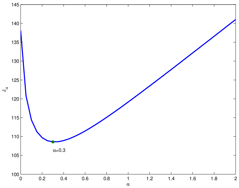
where $z_{i}(t,\xi)=x_{i}(t,\xi)-\sum_{j=1}^{5}x_{j}(t,\xi)/5$ . The performance functional was evaluated for a range of values of the uniform synchronization gain $\alpha$ in the interval $[0,2]$ . This cost is depicted in Figure 2(a) and its optimal value is attained when $\alpha=0.3$ .

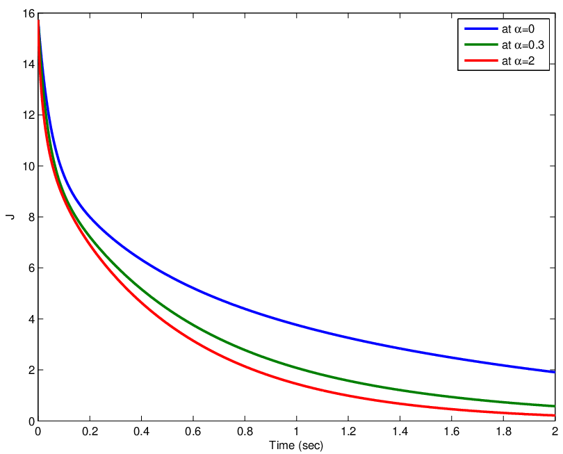
To examine the effects of the synchronization gain, the norm of the aggregate deviation from the mean was evaluated for $\alpha=0,0.3$ and $\alpha=2$ . The evolution of $|Z(t)|_{\mathbb{H}}$ is depicted in Figure 2(b). As expected, the higher the value of $\alpha$ , the faster the convergence. However, only the value $\alpha=0.3$ results in acceptable levels of the deviation from the mean and low values of the control cost.

IV-B Adaptive edge-dependent synchronization gains

The adaptive controller (8) was applied to the PDE with $a_{1}=0.1$ , $K\phi=5\times 10^{-4}\int_{0}^{1}b(\xi)\phi(\xi)\,\mathrm{d}\xi$ , $F=2K$ . The same initial conditions as in the constant gain case were used. The adaptations in (10) were implemented with an adaptive gain of $100$ and $\sigma=10^{-5}$ , i.e.

\dot{\alpha}_{ij}=\gamma\left[\left(\int_{0}^{1}b(\xi)x_{i}(t,\xi)\,\mathrm{d}\xi\right)\left(\int_{0}^{1}f(\xi)x_{ij}(t,\xi)\,\mathrm{d}\xi\right)-\sigma\alpha_{ij}\right],

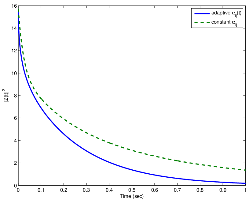
Figure 3(a) compares the adaptive to the constant edge-dependent gains case. The initial guesses of the adaptive edge-dependent gains were all taken to be $\alpha_{ij}(0)=1$ . The same values of $\alpha_{ij}=1$ were used for the constant case. The norm of the aggregate deviation from the mean exhibits an improved convergence to zero when adaptation of the edge-dependent gains is implemented.

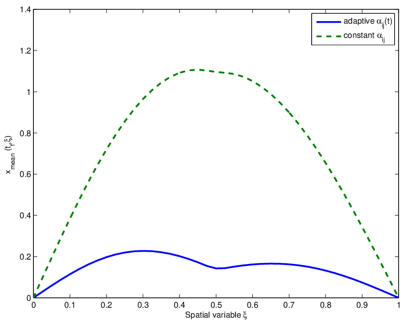
The spatial distribution of the mean state ( $x_{m}(t,\xi)=\sum_{i=1}^{5}x_{i}(t,\xi)/5$ ) is depicted at the final time $t=2$ for both the adaptive and constant gains case in Figure 3(b). It is observed that when adaptation is implemented, the mean state converges (pointwise) to zero faster than the constant case.

V Concluding remarks

In this note, a scheme for the adaptation of the synchronization gains used in the synchronization control of a class of networked DPS was proposed. The same framework allowed for the optimization of constant edge-dependent gains which was formulated as an optimal (linear quadratic) control problem of the associated aggregate system of the networked DPS. The proposed scheme required knowledge of the full state of the networked DPS. Such a case represents a baseline for the synchronization of networked DPS. The subsequent extension to output feedback, whereby each networked DPS can only transmit and receive partial state information provided by sensor measurement, will utilize the same abstract framework presented here.

References

[1] H. Su and X. Wang, Pinning control of complex networked systems: Synchronization, consensus and flocking of networked systems via pinning. Heidelberg: Springer, 2013.
[2] C. Wu and L. Chua, “Synchronization in an array of linearly coupled dynamical systems,” IEEE Trans. on Circuits and Systems I: Fundamental Theory and Applications, vol. 42, no. 8, pp. 430–447, 1995.
[3] H. Zhang, F. Lewis, and A. Das, “Optimal design for synchronization of cooperative systems: State feedback, observer and output feedback,” IEEE Trans. on Automatic Control, vol. 56, no. 8, pp. 1948–1952, 2011.
[4] T. Yang, S. Roy, Y. Wan, and A. Saberi, “Constructing consensus controllers for networks with identical general linear agents,” Internat. J. Robust Nonlinear Control, vol. 21, no. 11, pp. 1237–1256, 2011.
[5] T. Yang, A. A. Stoorvogel, and A. Saberi, “Consensus for multi-agent systems -synchronization and regulation for complex networks,” in Proc. of the American Control Conference, June 29 - July 1 2011, pp. 5312–5317.
[6] G. Chen and F. Lewis, “Distributed adaptive tracking control for synchronization of unknown networked lagrangian systems,” IEEE Trans. on Systems, Man, and Cybernetics, Part B: Cybernetics, vol. 41, no. 3, pp. 805–816, 2011.
[7] S.-J. Chung and J.-J. Slotine, “Cooperative robot control and concurrent synchronization of Lagrangian systems,” IEEE Trans. on Robotics, vol. 25, no. 3, pp. 686–700, 2009.
[8] J. Shan, “Six-degree-of-freedom synchronised adaptive learning control for spacecraft formation flying,” Control Theory Applications, IET, vol. 2, no. 10, pp. 930–949, 2008.
[9] H. Min, S. Wang, F. Sun, Z. Gao, and J. Zhang, “Decentralized adaptive attitude synchronization of spacecraft formation,” Systems & Control Letters, vol. 61(1), pp. 238–246, 2012.
[10] T. Krogstad and J. Gravdahl, “6-dof mutual synchronization of formation flying spacecraft,” in Proc. of the 45th IEEE Conference on Decision and Control, December 13-15 2006, pp. 5706–5711.
[11] W. Ren, “Distributed leaderless consensus algorithms for networked euler-lagrange systems,” International Journal of Control, vol. 82, no. 11, pp. 2137–2149, 2009.
[12] S. Chung, U. Ahsun, and J. Slotine, “Application of synchronization to formation flying spacecraft: Lagrangian approach,” AIAA Journal of guidance, control, and dynamics, vol. 32(2), pp. 512–526, 2009.
[13] M. A. Demetriou, “Synchronization and consensus controllers for a class of parabolic distributed parameter systems,” Systems & Control Letters, vol. 62, no. 1, pp. 70 – 76, 2013.
[14] ——, “Design of consensus and adaptive consensus filters for distributed parameter systems,” Automatica, vol. 46, no. 2, pp. 300 – 311, 2010.
[15] K. Wu and B.-S. Chen, “Synchronization of partial differential systems via diffusion coupling,” IEEE Trans. on Circuits and Systems I: Regular Papers, vol. 59, no. 11, pp. 2655–2668, 2012.
[16] K. Wang, Z. Teng, and H. Jiang, “Adaptive synchronization in an array of linearly coupled neural networks with reaction-–diffusion terms and time delays,” Communications in Nonlinear Science and Numerical Simulation, vol. 17, no. 10, pp. 3866 – 3875, 2012.
[17] B. Ambrosio and M. Aziz-Alaoui, “Synchronization and control of coupled reaction–diffusion systems of the fitzhugh–nagumo type,” Computers & Mathematics with Applications, vol. 64, no. 5, pp. 934 – 943, 2012.
[18] T. Li and B. Rao, “Exact Synchronization for a Coupled System of Wave Equations with Dirichlet Boundary Controls,” Chin. Ann. Math. Ser. B, vol. 34, no. 1, pp. 139–160, 2013.
[19] J. L. Lions, Optimal Control of Systems Governed by Partial Differential Equations. NY: Springer-Verlag, 1971.
[20] R. E. Showalter, Hilbert Space Methods for Partial Differential Equations. London: Pitman, 1977.
[21] Y. Liu, Y. Jia, J. Du, and S. Yuan, “Dynamic output feedback control for consensus of multi-agent systems: An $H_{\infty}$ approach,” in Proc. of the American Control Conference, June 10-12 2009, pp. 4470–4475.
[22] C. Godsil and G. Royle, Algebraic graph theory, ser. Graduate Texts in Mathematics. New York: Springer-Verlag, 2001, vol. 207.
[23] R. F. Curtain and H. J. Zwart, An Introduction to Infinite Dimensional Linear Systems Theory, ser. Texts in Applied Mathematics, Vol. 21. Berlin: Springer-Verlag, 1995.
[24] M. Tucsnak and G. Weiss, Observation and Control for Operator Semigroups. Basel-Boston-Berlin: Birkhäuser Verlag AG, 2009.
[25] W. Yu, P. De Lellis, G. Chen, M. Di Bernardo, and J. Kurths, “Distributed adaptive control of synchronization in complex networks,” IEEE Transactions on Automatic Control, vol. 57, no. 8, pp. 2153–2158, 2012.
[26] P. De Lellis, M. Di Bernardo, and F. Garofalo, “Novel decentralized adaptive strategies for the synchronization of complex networks,” Automatica, vol. 45, pp. 1312–1318, 2009.
[27] ——, “Synchronization of complex networks through local adaptive coupling,” Chaos, vol. 18(3), p. 037110, 2008.
[28] P. De Lellis, M. Di Bernardo, F. Garofalo, and M. Porfiri, “Evolution of complex networks via edge snapping,” IEEE Trans. on Circuits and Systems I: Regular Papers, vol. 57(8), pp. 2132–2143, 2010.
[29] P. A. Ioannou and J. Sun, Robust Adaptive Control. Englewood Cliffs, NJ: Prentice Hall, 1995.
[30] M. Böhm, M. A. Demetriou, S. Reich, and I. G. Rosen, “Model reference adaptive control of distributed parameter systems,” SIAM J. Control and Optimization, vol. 36(1), pp. 33–81, 1998.
[31] F. Fahroo and K. Ito, “Optimal absorption design for damped elastic systems,” in Proc. of the American Control Conference, Minneapolis, Minnesota, USA, June 14-16 2006, pp. 2459 – 2464.
[32] ——, “Optimal absorption design and sensitivity of eigenvalues,” in Proc. of the 45th IEEE Conference on Decision and Control, San Diego, CA, USA, December 13-15 2006, pp. 2459–2464.