Generic instabilities in a fluid membrane coupled to a thin layer of ordered active polar fluid
Abstract
We develop an effective two-dimensional coarse-grained description for the coupled system of a planar fluid membrane anchored to a thin layer of polar ordered active fluid below. The macroscopic orientation of the active fluid layer is assumed to be perpendicular to the attached membrane. We demonstrate that activity or nonequilibrium drive of the active fluid makes such a system generically linearly unstable for either signature of a model parameter that characterises the strength of activity. Depending upon boundary conditions and within a range of the model parameters, underdamped propagating waves may be present in our model. We discuss the phenomenological significance of our results.
I Introduction
Studies on fluid membranes have a long tradition in equilibrium statistical mechanics [1]. Coarse-grained descriptions of a fluid membrane, parametrised by its tension, bending modulus and spontaneous curvature [2], provide a quantitatively accurate description of thermal fluctuations of fluid membranes. Plasma membranes in eukaryotic cells, ignoring their bilayer structure and internal complications, are broadly described by a fluid membrane, typically attached to a layer of cortical actin filaments. Understanding of the mechanical responses of in-vivo eukaryotic cells to external stimuli, in which both the cell membrane and actin filaments are expected to play crucial roles, remains a highly challenging subject due to the underlying structural complexities of a cell. It is, therefore, useful to theoretically consider or experimentally design simple in-vitro systems involving membranes and actin filaments, whose macroscopic physical properties may be understood or analysed in a straightforward manner. In the spirit of this minimalist approach, in this article we construct a coarse-grained two-dimensional () hydrodynamic description of the coupled dynamics of a fluid membrane and a macroscopically polar ordered active fluid layer anchored locally normally to it. In general, a combined system of a plasma membrane and an anchored layer of actin filaments executes dynamics that is distinctly nonequilibrium [3, 4]. Hence, thermal equilibrium models of fluid membrane do not suffice as meaningful descriptions of such a system.
There have been several recent studies on the various aspects of out of equilibrium dynamics of fluid membranes in systems with biological relevance; see, e.g., Refs. [5, 6, 7, 8, 9, 10, 11, 12]. In the present work, we complement the existing results and consider a thin layer of active fluid with the active particles normally anchored to a fluid membrane at length scales much larger than the lengths of the individual polar particles (e.g., actin filaments) and layer thickness with polar ordering, for which a generic coarse-grained continuum two-dimensional () description should suffice. The nonequilibrium aspect of the active fluid dynamics is modelled in terms of an active contribution to the stress tensor, called active stress (nonequilibrium stress), proposed and elucidated in Refs. [13, 14]; see also Ref. [15] for recent development in the subject. It is assumed that the active fluid layer is covered by a fluid membrane on one side, which is parametrised by its surface tension and bending stiffness only. Here, we systematically construct a set of thickness-averaged effective coarse-grained coupled dynamical equations for our model, by following the approaches outlined in Refs. [9, 11]. We use our equations to study linear instabilities about the assumed polar ordered state. We find that the system shows generic instability for both signatures of , a parameter that characterises the strength of the active stress in the model. In addition, under certain circumstances and depending upon the boundary conditions imposed, the system may display underdamped propagating waves as well. While our calculational framework is closely related to Ref. [11] (see also Ref. [9]), the system under consideration here is quite different from those in Refs. [9, 11] in having a macroscopic orientation different from Refs. [9, 11]. Furthermore, we include in our model a second active species, represented by a local active density, that exists on the membrane. This may, for instance, model proteins that bind with the actin filaments and facilitate actin polymerisation.
Our model, although lacks many biological details, is motivated by the consideration that the cortical actin layer is generally isotropic in-plane, and is anchored to the cell membrane. Technically, if the underlying polar particles are actin filaments, our description should be valid for time scales larger than the unbinding time scale of the cross-linking proteins of the actin filaments, so that the actin network behaves like a fluid. Furthermore, our model should be useful as a starting point for theoretical descriptions for recent in-vitro experiments [16, 17, 18]. Despite the technical difficulties involved, our results described here may in principle be tested by performing controlled experiments on thin confined actin layers, grafted normally on both the bounding surfaces with a sample thickness much smaller than the correlation length in the thin direction. The rest of the paper is organised as follow: In Sec. II, we set up our model, specify the boundary conditions and derive the equations of motion. In Sec. III we perform linear stability analysis on our model equations. In Sec. IV we conclude and discuss our results.
II Construction of the model and the equations of motion
Assuming a planar membrane for simplicity, we consider a thin layer of ordered active fluid of viscosity , attached to the membrane, spread in the plane and thin in the -direction. Our study begins with the three-dimensional () hydrodynamic description of a polar ordered state in this model system; the relevant dynamical fields include (we assume an incompressible system) local velocity field , a polarisation field , a unit vector that describes any local orientational order, concentration of the active particles and which describes an active species density that exists on the membrane. Our system is confined between the surfaces and . We study small fluctuations about a chosen reference state given by . Our aim is to construct an effective description of the combined active polar fluid-membrane dynamics, such that any -dependence is averaged out and the effective dynamical variables depend only on . Similar to Ref. [11], we consider two different versions of our model: (i) Model I: The fluid membrane-active fluid combine rests on a solid substrate below, and (ii) Model II: The system is embedded inside a bulk isotropic passive fluid having a viscosity , assumed to be much smaller than . As discussed in details in Ref. [11], the two cases are physically different. The solid substrate below introduces friction and, hence, the momentum (or the hydrodynamic velocity for an incompressible system) is no longer a conserved variable. In contrast, with a bulk fluid surrounding the system there is no friction at the interface, and therefore, the momentum density (equivalently, for an incompressible system) is a conserved variable. Furthermore, the solid substrate breaks the full three-dimensional () rotational invariance of the problem, where as, when there is an embedding bulk fluid, the system remains invariant under the full rotational invariance (see below). We separately discuss Model I and Model II in details below, and construct coupled equations motion for the membrane height field, velocity field of the active fluid, polar particle concentration and the active density on the membrane.
II.1 Model I: The membrane active gel combine bounded by a solid substrate below
II.1.1 Construction of the model and the free energy functional
Model I, where the fluid membrane-active fluid layer combine rests on a fully flat solid substrate (see Fig. 1), is relevant in the context of in-vitro experiments discussed, e.g., in Ref. [16].

In order to set up the equations of motion we first consider the form of the relevant free energy functional that gives the energy of a configuration defined by height field (we set , since it is a rigid surface below) and polarisation . The form of may be inferred by using symmetry arguments. First of all, the presence of the solid substrate below makes the system invariant under in-plane (-plane) rotation and the translation (we neglect any interaction between the membrane and the bottom solid surface, which is reasonable if the average thickness of the intervening active fluid is not too small). However, there is no invariance under a full rotation. As discussed in Ref. [11, 13], the symmetry considerations as above dictates that the leading order (in gradients) coupling between and and the height of the membrane should be a term of the form , where . The chosen form of the coupling is determined by the invariance under in-plane rotation and translation along . This is a polar term, since it has no symmetry. Further, it violates the symmetry as well, which is admissible since the active fluid is anchored only on one side of the membrane. Further, the configuration energy of the membrane is assumed to be determined by its local curvature and surface tension. Lastly, the free energy of the active polar particles is given by the Frank free energy for nematic liquid crystals [19]. Thus we have
| (1) | |||||
where and are the surface tension and bending modulus of the membrane, is the spatial average of , is the osmotic modulus of the membrane bound active density for small , is the temperature, and are coupling constants (all chosen to be positive) for the bilinear terms. We impose . The Frank free energy is considered in the limit of equal Frank’s constants, denoted by above. We have used the Monge gauge [20] for the membrane height field in the free energy functional (1) and have kept only the terms which are either quadratic or bilinear in the fields. Operator and are the and Laplacians respectively. All the parameters in the model are chosen in such a way, that a stable spatially uniform equilibrium phase [21] (at zero activity) is ensured, e.g., are assumed to be positive. Note that the free energy functional (1), with , appears similar to the corresponding free energy functional used in Ref. [11]. This is essentially due to the polar nature of the systems considered in Ref. [11] as well as here. A careful consideration, however, reveals differences. For instance, the free energy and the corresponding macroscopic behaviour in Ref. [11] have in-plane anisotropy (although anisotropic coefficients were not used in the free energy functional there, in order to reduce the algebraic complications), due to the chosen ordered state with , where as the present model is invariant under rotation in the -plane. Due to the macroscopic orientation along the -direction, our system is, however, generally anisotropic in the -direction, resulting into anisotropic coupling constants, e.g., Frank’s elastic constants. For reasons of simplicity and analytical tractability, we choose to ignore such complications. Higher order non-linearities should also reflect this anisotropy; since we restrict ourselves only up to terms bilinear in the fields, we are not concerned by such issues here.
II.1.2 Boundary conditions
Having constructed the free energy above, we now consider the boundary conditions to be imposed: (i) First of all, the solid substrate below introduces friction; consequently, the relevant boundary condition on the velocity field at is the no-slip boundary condition on : , where and no penetration on : at , (ii) Further, local orientation is constrained to be normal to the plane and the local normal at , and finally (iii) vanishing of the shear stress and the normal stress balance at . Assuming that the relevant nonequilibrium intrinsic stress field of the active particles [15] is , the vanishing of the shear stress at yields
| (2) |
which, in the thin film approximation where is assumed to be small and may be neglected, reduces to
| (3) |
at , where . The kinematic boundary condition together with the incompressibility of the active fluid connects with the flow:
| (4) |
Considering active particles being normally grafted onto the membrane, we have . This yields, for small fluctuations of the membrane, at . Here is the unit normal to the membrane surface, which in the Monge gauge is given by to the lowest order in height fluctuations. Since the surface at is flat (a rigid solid surface), the boundary condition on at is .
II.1.3 Active stresses and the dynamical equations of motion
The stress field of the active particles [15], called active stress below, is of the form
| (5) |
In the context of eukaryotic cells, the constant parameter , gives a measure of the free energy available from the hydrolysis of the Adenosine Triphosphate (ATP) molecules inside the cell. For bulk polar active fluids, with , is said to be contractile or extensile for or [14]; its numerical value characterises the strength of the active stress field. A local imbalance of the membrane-bound density creates a local normal stress component that is assumed to be active. In (5) we have ignored any coupling between and the local curvature . Thus there are two different sources for active stresses, the orientation field and the local density . The magnitudes of the couplings and (both assumed to be positive here) describe the relative strengths of the different contributions to the active stress (5). In addition, we assume not to have any significant -dependence. Further, since we are interested in the effective long wavelength dynamics in the -plane, in what follows below, we use a linear profile for that clearly satisfies the boundary conditions imposed on and use this form to calculate -averaged active stresses [9, 22] from (5): In particular we have for the shear active stress
| (6) |
where implies -averaging of any quantity, . This allows us to borrow the methods of Refs. [11, 9] directly for the present problem. How good is it expected to be? It is well-known [12, 23], at a critical thickness , a Frederik-like spontaneous flow instability sets in. In the model of Ref. [12], both the confining surfaces are held fixed (non-fluctuating) and at both the top and bottom boundaries, such that the profiles of may be written as a sum of appropriate trigonometric functions of that obey at automatically. With this, the instability at , that depends upon , manifests itself explicitly. If the top surface becomes a flexible surface with small fluctuations, we expect a small departure from the -dependent profiles for in Ref. [12]. Therefore, our choice of a linear profile should not be a good approximation for near ; we expect our results here will be meaningful in the limit such that the Frederik-like spontaneous flow instabilities are strongly suppressed and consequently, a -averaged description is physically valid. Before embarking on our calculations, let us compare with Ref. [11] briefly, where fluctuations about a state is studied. There, is constrained to have prescribed values at the boundaries (0 and , at and respectively), where as remains unconstrained at the boundaries. As a result, is slaved to and drops out of the effective description that was constructed. In the present model, for the same reason, and , having specified values at , are slaved to and drop out of the eventual effective theory (moreover, to the lowest order in smallness, and, hence has no time evolution). Thus we are left out with and as the slow variables that describe the dynamics of the model in the long time limit.
As we shall see below, a full solution of the dynamics of the model at hand entails solving for the coupled dynamics of and (this enters through the conservation of the active particles, see below). Neglecting inertia, which is a good approximation for active particles with small masses (equivalently, low Reynolds number flows) and within the lubrication approximation, the velocity field satisfies the generalised Stokes equation that now includes the active stress term. In particular, the in-plane component obeys
| (7) |
where , . For the -component of Eq. (7) we use the lubrication approximation for (i.e, ) in the thin film limit, which then yields
| (8) |
where we have linearised about and . Equation (8) can be integrated over to solve for the pressure . The constant of integration is to be fixed by the condition of normal stress balance. The pressure at the location of the membrane is balanced by the total normal stress at . This includes the elastic force of the membrane and the active stress due to the active density. Thus, is obtained as
| (9) |
where is the elastic contribution to the stress which can be derived from the free energy as , where we have replaced by its -averaged form. Substituting for from the above in the linearised Stokes Eq. (7) for , integrating twice with respect to and using boundary conditions (i) at and (ii) at , , we obtain
| (10) | |||||
We now use incompressibility of the fluid, giving to obtain by using the kinematic boundary condition (4)
| (11) | |||||
where we have linearised about the mean membrane height . Being a conserved density, the active density follows a model B (in the nomenclature of Ref. [24]) type equation, together with advection. For an incompressible fluid and up to linear order the equation takes the form (we have set a kinetic coefficient to unity for simplicity and without any loss of generality)
| (12) |
where . The dynamics of concentration follows the advection equation
| (13) |
where is a drift velocity. Writing , where now refers to the (small) fluctuations of the local active particle concentration from , to the linear order in fluctuations (i.e., in or and ), follows the equation
| (14) |
where has been replaced by its -averaged expression. Thus, the dynamics of is slaved to -fluctuations. Notice that at the linearised level and to the lowest order in smallness, only , the average active particle concentration in the active fluid film, and not the fluctuations in , enters into the dynamics of and . In contrast, the dynamics of itself is affected by fluctuations in and . Hence, we ignore the dynamics of and replace it by in the equations for and for the remaining part of this article. Under the -averaged description used here, there is no independent dynamics of . Thus, Eqs. (11) and (12) for and respectively together describe the effective dynamics of the membrane-active fluid layer combine. This is in agreement with our qualitative arguments above. Equations (11) and (12) may be conveniently written in terms of spatially Fourier-transformed variables, which are used below to elucidate the linear instabilities:
| (15) |
and
| (16) |
where and are spatial Fourier transforms of and ; is a Fourier wavevector.
II.2 Model II: The membrane active gel combine bounded by a fluid interface below
II.2.1 Construction of the model and the free energy functional
Our calculation here broadly follows the framework outlined above. However, there are important differences in details, owing to symmetry considerations and boundary condition. We start by considering the free energy functional of the system. Assuming the system to be confined between and , should be a functional of , and . This describes the energy of the system in a given configuration defined by , and . Just as for , its form may be directly inferred from symmetry considerations. It must generally be invariant under an arbitrary tilt (equivalently a rotation) of the confining surfaces, where is an arbitrary vector and is a radius vector. At this stage, similar to Ref. [11], in order to simplify the ensuing algebra, we assume that the interfacial tension of the lower surface is large enough (formally diverging) so that its fluctuations are strongly suppressed, and thus, drops out of the dynamical description in this limit. Although this is not likely to be directly realisable in any in-vivo or in-vitro situations, they should nevertheless serve as a good starting point for more refined and detailed theoretical modeling. To set our notations simpler, we set and below. See Fig. 2 below for a schematic representation of our model.

The tilt symmetry in Model II dictates that the most leading order (in gradients) coupling bilinear in and should be through the local curvature. Hence, assuming small membrane fluctuations, the most leading order term that contributes to the relevant free energy functional should be of the form . The form of this -coupling term is a crucial difference with [see (1) above]; in order to avoid introducing a large number of symbols, we continue to use the same symbols as in (1). Despite the structural differences owing to symmetry considerations, the and couplings reflect the polarity of the system, similar to Model I. We continue to represent the density of the active species on the membrane by . Similar to (1), the free energy of the active polar particles is given by the Frank free energy, which we consider in the limit of equal Frank’s constants, denoted by below, ignoring any anisotropy for simplicity. Thus the free energy functional of the combined system of a fluid membrane, active fluid layer and an active density on the membrane is given by
| (17) | |||||
where different symbols above have the same significance as in (1). We continue to impose . Similar to Model I, we have used the Monge gauge [20] above and have kept only the terms which are either quadratic or bilinear in the fields. As before, all the parameters in the model are chosen in such a way, that a stable spatially uniform equilibrium phase [21] (at zero activity, ) is ensured. Our previous discussions on the differences between and the corresponding free energy functional in Ref. [11] similarly applies to above and its corresponding free energy functional in Ref. [11].
II.2.2 Boundary conditions
Next, we specify the boundary conditions on the system: (i) At the interfaces ( and 0) polarisation is constrained to be perpendicular to the plane and the local tangent plane on the surfaces , i.e., at , where is the local normal at in the Monge gauge (see above; equivalently at for small membrane fluctuations and at ) and at ; these are identical to the boundary conditions used in Model I above, and (ii) continuity of the shear stress at and 0, which for reduces to the condition (3) at and at , where . Notice the difference between the boundary conditions on at for Model I and Model II: For Model I, at (no-slip boundary condition), where as for Model II, at . We shall see below that this difference in the boundary conditions is responsible for the differences in the fluctuation spectra that we obtain. The dynamics of the height field is again determined by the kinematic boundary condition (4).
II.2.3 The dynamical equations of motion
We continue to use the active stress defined above (5) that determines the active stress in the system. Similar to Model I above, we assume no significant -dependence of concentration , use a linear profile for that satisfies the boundary conditions imposed on and use this form to calculate -averaged active stresses from (5). The validity of this approach should still be the same as for Model I, the average thickness , the critical thickness at which a spontaneous flow transition akin to the Frederiks transition of equilibrium nematics. For reasons similar to Model I, and will appear as the relevant dynamical fields in our effective description which we work out below.
As in the previous section, we use the generalised Stokes Eq. for velocity . We further use the Lubrication approximation for in the thin film limit yielding an equation identical to Eq. (8). This can be integrated over to solve for the pressure . The constant of integration is to be fixed by the condition of normal stress balance. The pressure at the location of the membrane is balanced by the total normal stress at . This includes the elastic force of the membrane and the active stress due to the active density. Thus, is obtained as
| (18) |
where is the elastic contribution to the stress which can be derived from the free energy as .
Since does not satisfy the no-slip boundary condition at any of the confining surfaces at and , unlike Model I, cannot be obtained by using the lubrication approximation on the corresponding Stokes’ equation. Instead, we note that the zero shear stress boundary conditions at allows for a non-zero that is independent of , unlike Model I, which cannot have a -independent non-zero . To proceed further and in the spirit of a -averaged description, we assume that has, in addition to a -independent part, a -dependent part with a quadratic -dependence , such that the boundary conditions on are obviously satisfied. Such an approach is physically meaningful over a length-scale that is much larger than , i.e., in terms of the corresponding Fourier wavevector , (a more formal derivation of the expression for is given in Appendix I). With this we obtain in the Fourier space (a subscript refers variables in the Fourier space)
| (19) | |||||
This, together with the incompressibility condition, then yields in the Fourier space
| (20) | |||||
The dynamics of and follows the same equations (12) and (14) as for Model I. Again as in Model I, the dynamics of is slaved to that of -fluctuations in the lowest order in smallness. Thus, equations (20) and (16) together describe the effective dynamics of Model II in the long wavelength limit.
III Linear stability of polar ordered uniform states
Having derived all the governing equations for the dynamics of Model I and Model II, we perform linear stability analyses of small fluctuations around the chosen ordered states.
III.1 Stability analysis for Model I
The linear stability of the chosen ordered state may easily be ascertained by calculating the eigenvalues of the stability matrix constructed from equations (15) and (16): The eigenvalues are rather lengthy and are available in Appendix II. Regardless of the complicated structure of the eigenvalues as given in Eq. (VI), we note that they vanish for , a consequence of screening of the hydrodynamic interactions due to the presence of the solid substrate below which generates friction. While straightforward analysis of the eigenvalues (VI) requires considerable algebraic manipulations, despite the complexity of the eigenvalues (VI) we can make the following observations: (i) There are no underdamped propagating modes, (ii) the system becomes unstable for either signature of . The latter feature manifests itself clearly if we ignore the active density from the dynamics and analyse only the dynamics of . We separately analyse for (i) and (ii) .
Setting , there is only one eigenvalue:
| (21) |
Thus for any (extensile active stress), the system is unstable at , the lowest order in wavevector , but becomes stable at . For a system with a linear lateral size , this yields an instability condition , where the critical linear size is given by
| (22) |
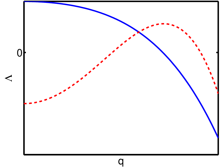
Thus, for a given and , there is always a system size , at which the instability will show up. We can make an order of magnitude estimation for as follows: We take , a typical thickness of a cortical actin layer in a cell, [11], for an ordered system with a typical active particle size , , . This then yields a typical , smaller than the linear dimension of a cell. In contrast, for (contractile active stress), there are no instabilities at , but the system becomes unstable at as soon as as exceeds a critical thickness given by . Using the values of the parameters as above we find, , smaller than the typical thickness of a cortical actin layer. This, however, does not impose any condition on system size . Systems with a linear dimension larger than or with an average thickness larger than are expected to display the linear instabilities obtained above. Of course, the system is stable at high enough , the bending modulus stabilises the system regardless of the sign of . The instabilities for either signature of may be understood as follows. In the underlying full model, there is only one nonequilibrium term, which is the active stress. In the resulting description, it contributes to the dynamics of through (a) the analogue of the active stress (5) and (b) the active pressure. From the structure of the generalised Stokes Eq. (7) for , the active pressure term balances the usual pressure, where as in the Stokes Eq. for the pressure and the active stress together balance the viscous stress term. Therefore, the active pressure and the active stress terms appear with opposite signs in and hence in through the incompressibility condition, and therefore in Eq. (15) for . This leads to the instabilities for both signatures of in the dynamics of . A schematic diagram of the eigenvalue when for both signs of is given in Fig. 3.

.
he instabilities are due to the active stress term , since the second active term has been set to zero by setting . The opposite limit may also be examined by setting , leaving the active density-dependent term in the active stress expression (5) on the membrane as the only source of active stress in the problem. One obtains coupled dynamical equations for and . The eigenvalues of the stability matrix are given by
| (23) |
Thus, comes with opposite signs in the two eigenvalues. Hence, for a fixed sign of there are instabilities associated with either signature of . However, the notable difference with is that the instabilities now occur only at , much higher than . In contrast, there is no instability , unlike the instabilities which occur in the previous case (). In particular with positive , when , there is instability at for any value of , where as when , there is instability at provided exceeds a critical value defined by . More generally, in the present case, the cross-coupling between and is responsible for the instabilities for both signatures of . While our detailed analysis of the eigenvalues above rests on simplifying steps effectively involving keeping only one term of the active stress expression (5) at a time, we expect the general conclusion on the presence of instability for both signatures of should be valid. In particular, since the governing equations of motion are linear, a combination of the instabilities elucidated above should be generally observed for proper choices of the model parameters when both and are non-zero. Finally, for high enough , the system should always be stabilised by the curvature contributions (not shown here).
III.2 Stability analysis of Model II
The instabilities to the uniform state may be obtained by calculating the eigenvalues of the stability matrix from the equations (16) and (20). The full expressions of the eigenvalues are given in Appendix VII, which are rather lengthy. However, we use their forms up to for our analyses in this Section below. These instabilities have both qualitative similarities and dissimilarities with those in Model I which are discussed in details below. As before, we analyse the eigenvalues for two special cases - (i) , and (ii) .
With , the height field remains the only relevant field and we obtain
| (24) |
Thus, with (extensile), the system is unstable at , but stable at or higher. Similar to Model I, the instability condition (24) imposes a condition on the system size for instability: One must have
| (25) |
for instability. Condition (25) is analogous to the condition (22) for Model I above. In contrast, with , (contractile) the system is stable at , but becomes unstable at if . As for Model I, there is no condition on the system size for occurrence of the instability. Thus the system may display instabilities for both signatures of , again very similar to the corresponding result from Model I. The physical origin of these instabilities are again same as that for Model I, viz, that the active stress (5), with , contributes to the analogue of (5) and also makes an active contribution to the pressure (18). For high enough , the instabilities are always suppressed by the curvature contribution, regardless of the signature of . A schematic diagram of the eigenvalue when for both signs of is given in Fig. 4.
.
The other limiting case with , but turns out to be qualitatively different from its counterpart in Model I. There are two eigenvalues, for there are now two dynamical fields, and . The eigenvalues obtained are available in Appendix III; to the lowest order in they are
| (26) |
From (26) note that various scenarios are possible, which we consider by taking various limits (we assume for simplicity). Two different possibilities exist: (a) When then,
- •
If , there is an instability at with positive .
- •
If , the system is unstable for with an instability at .
There are no underdamped propagating modes in the system. In contrast (b) when then
- •
There are underdamped propagating modes for any with dispersion proportional to and speed depending linearly on . In this case, however, there are no instabilities.
- •
When , there are instabilities at when .
Similar to Model I, in a general situation with both and being non-zero, a combination of all the linear instabilities discussed above should be displayed by the system with appropriate choices for the model parameters.
Let us now look at the similarities and differences between the mode spectra and instabilities in Model I and Model II. When the active density is absent, both Model I and II yield generic instabilities for both signatures of for the dynamics of . There are, however, significant differences too. At a technical level, first of all, in Model II, the eigenvalues do not vanish for . This is a consequence of the Stokesian dynamics for the velocity field; see Ref. [11] for more discussions in an analogous problem. This is in contrast to Model I, where hydrodynamic interactions are screened and the eigenvalues smoothly go over to zero as . There are other differences which manifest when , leading to the existence of underdamped propagating waves in Model II, unlike Model I where there is no such propagating mode. This is formally a consequence of the Stokesian dynamics together with hydrodynamic interactions in Model II: The active stress contribution from the density to the dynamics od for Model II yields leading order contribution (along with other leading order terms), where as for Model I, such contributions are always subleading. This difference leads to the existence of underdamped propagating modes for in Model II, a possibility that does not exist in Model I.
IV Summary and outlook
In summary, thus, we have formulated an effective description for the coupled dynamics of small fluctuations of height and active species density in a thin layer of fluid membrane-active fluid combine about a reference state with , being the thin direction. Linear stability analysis of the model reveals possibilities for instabilities for either signature of . These instabilities may be moving, as in our Model I with a solid substrate below, or static (or localised) as in our Model II with the membrane-active fluid combine being embedded in a bulk fluid. We have analysed the roles played by the two sources of nonequilibrium active stresses separately in generating the linear instabilities in our models. Our results amply highlight the role of boundary conditions in determining the long wavelength properties of the system.
Direct comparisons of our results with the available experimental results are difficult, mainly due to the simplified, minimalist nature of our model and (to our knowledge) the lack of precise measurements of membrane fluctuations. Nevertheless, Ref. [18] reports an unusually low value for the surface tension obtained for a cytoskeletal actin-myosin network encapsulated in giant liposomes by fitting the membrane fluctuations with the Helfrich model, which does not take active effects into account. While the presence of active stresses and the consequent instabilities may well be responsible in such an unusual value for the (effective) surface tension, we cannot say anything conclusively at present. Further experimental works may be necessary for resolving this issue definitively. However, regardless of the present status of the experimental results, in-vitro systems such as those used in Refs. [17, 18] may in principle be used to study our theoretical predictions. Our estimation of and , while indicating that a system size smaller than a typical eukaryotic cell and/or thinner than a cortical actin layer should be linearly unstable and will not stay in a linearly ordered state, are only suggestive and any quantitative accuracy is not expected. Since our calculational framework is applicable only when the average system thickness is much smaller than the threshold of the spontaneous flow transition, we cannot comment on the linear stability of system near the threshold. We note here that the results from our Model II are largely of theoretical interests. This is primarily because of our assumption of a diverging interfacial tension at the bottom surface of the system. In a real situation when the interfacial tension is generically finite, the bottom surface fluctuates, and one generally has fluctuations of both the mean height and thickness . Our model does not capture such features. Full calculations are needed to capture these additional features. Nevertheless, qualitative aspects of our results should be visible in more refined calculations.
Our results are complementary to those from related theoretical works. For instance, Ref. [6] in a coarse-grained linearised model in terms of the membrane height field and the active protein density ( in our notation) showed, along with linear instabilities, how the membrane gets a mean velocity in the model: is non-zero and taken to be proportional to in their model, which is physically due to the protruding forces coming from the polymerisation of the normally anchored actin filaments. While we do not have any overall movement of the membrane in our model, this can be included easily in our model by an explicit addition of a term proportional to in Eqs. (20) and (11). However, this should be done with caution: If there is a constant (say, upward according to our Fig. 2) velocity of the membrane, the top-to-bottom distance will rise indefinitely and our -averaged effective description will become invalid eventually. In a related model, Ref. [7] extends the model of Ref. [6] by including the effects of contractile forces due to molecular motors such as myosin, leading to generic travelling waves in the membrane. In contrast, our model (Model I) displays no underdamped travelling waves. Unlike Refs. [6, 7], our model explicitly incorporates orientation fluctuation-dependent active stresses and displays instability for both contractile and extensile active stresses (both signs of ). Lastly, instead of a one-component active polar species one may consider active protein pumps, modelled by densities of upward and downward pumps, together with permeation [5]. These are known to introduce travelling waves or instabilities in the membrane, depending on details (e.g., local structural or functional asymmetries). We hope our work will induce further theoretical and experimental studies along these directions.
V Appendix I: Alternative derivation of in Model II
The in-plane velocity for Model II may be obtained using the Green’s function technique. Let Green’s function for Eq. (7) such that it satisfies an equation
| (27) |
Further, obeys the same boundary conditions as for Model II. Then for , the solutions for are given by
| (28) | |||||
| (29) |
From the boundary conditions on , we obtain at and at , where is any function of and , which is to be determined. Thus we obtain
| (30) | |||||
| (31) |
Integrating Eq. (27) we get
| (32) |
This along with the continuity of the Green’s function solution i.e., gives us
| (33) | |||||
| (34) |
Now we can write as
| (35) | |||||
| (36) |
where the kernel (in the Fourier space) can be evaluated using Eqs. (5) and (18). Eliminating using , the final expression for comes out to be (in the limit and retaining the lowest order terms
| (37) | |||||
upon linearisation, where is a two dimensional fourier wavevector. This is same as Eq. (19).
VI Appendix II: Eigenvalues of the stability matrix in Model I
The eigenvalues are formally given by
where
where are the different elements of the stability matrix .
VII Appendix III: Eigenvalues of the stability matrix in Model II
The eigenvalues of the stability matrix for and in Model II can be written explicitly as
| (39) | |||||
Expanding the above to yields Eq. (26).
VIII Acknowledgement
AB gratefully acknowledges partial financial support in the form of the Max-Planck Partner Group at the Saha Institute of Nuclear Physics, Calcutta, funded jointly by the Max-Planck- Gesellschaft (Germany) and the Department of Science and Technology (India) through the Partner Group programme (2009).
References
- [1] U. Seifert, Adv. Phys., 46, 13 (1997); S. Ramaswamy, J. Prost, and T.C. Lubensky, Europhys. Lett., 27, 285 (1994); 23, 271 (1993).
- [2] W. Helfrich, J. Phys. (France), 46, 1263 (1985); H.J. Deuling and W. Helfrich, ibid. 37, 1335 (1976).
- [3] S. Tuvia, A. Almagor, A. Bitler, S. Levin, R. Korenstein, and S. Yedgar, Proc. Natl. Acad. Sci. U.S.A. 94, 5045 (1997).
- [4] M. Edidin, Annu. Rev. Biophys. Bioeng. 3, 179 (1974).
- [5] J.-B. Manneville, P. Bassereau, S. Ramaswamy, and J. Prost, Phys. Rev. E 64, 021908 (2001).
- [6] N. S. Gov and A. Gopinathan, Biophys. J. 90, 454 (2006).
- [7] R. Shlomovitz and N. S. Gov, Phys. Rev. Lett. 98, 168103 (2007).
- [8] J. Zimmermann et al, Biophys. J 102, 287 (2012).
- [9] S. Sankararaman and S. Ramaswamy, Phys. Rev. Lett. 102, 118107 (2009).
- [10] N. Sarkar and A. Basu, Eur. Phys. J E 34, 44 (2011).
- [11] N. Sarkar and A. Basu, Eur. Phys. J. E 35, 115 (2012).
- [12] A. Basu, J.-F Joanny, F. Jülicher and J. Prost, New J. Phys. 14, 115001 (2012).
- [13] R.A. Simha, S. Ramaswamy, Phys. Rev. Lett. 89, 058101 (2002).
- [14] K. Kruse, J.F. Joanny, F. Julicher, J. Prost and K. Sekimoto, Eur. Phys. J. E 16, 5 (2005).
- [15] S. Ramaswamy, Annu. Rev. Cond. Matt. Phys. 1, 323 (2010); G.I. Menon, arXiv:1003.2032; J.-F. Joanny, J. Prost, in Biological Physics, Poincar´e Seminar 2009, edited by B. Duplantier, V. Rivasseau (Springer, 2009) pp. 1-32; M. C. Marchetti et al, arXiv:1207.2929.
- [16] B. Brough et al, Soft Matter 3, 541 (2007); C. Mohrdieck et al, Small 3, 1015 (2007).
- [17] J. Pécréaux, H.-G. Döbereiner, J. Prost, J.-F. Joanny, and P. Bassereau, Eur. Phys. J. E 13, 277 (2004).
- [18] F.-C. Tsai, B. Stuhrmann and G. H. Koendrink, Langmuir 27, 10061 (2011).
- [19] P.-G. de Gennes and J. Prost, The Physics of Liquid Crystals, Clarendon, Oxford (1993).
- [20] Statistical Mechanics of Membranes and Surfaces, edited by D. Nelson, T. Piran, and S. Weinberg World Scientific, Singapore (1989).
- [21] T. C. Lubensky and F. C. MacKintosh, Phys. Rev. Lett. 71, 1565 (1993).
- [22] H.A. Stone, in Nonlinear PDEs in Condensed Matter and Reactive Flows, NATO Science Series C: Mathematical and Physical Sciences, 569, H. Berestycki and Y. Pomeau eds., Kluwer Academic, Dordrecht, The Netherlands (2002); A. Oron, S.H. Davis and S.G. Bankoff, Rev. Mod. Phys. 69, 931 (1997).
- [23] R. Voituriez, J.-F. Joanny and J. Prost, Euro. Phys. Lett., 70, 404 (2005).
- [24] P.C. Hohenberg and B.I. Halperin, Rev. Mod. Phys. 49, 435 (1977).