Video Human Segmentation using Fuzzy Object Models and its Application to Body Pose Estimation of Toddlers for Behavior Studiest2
Abstract
Video object segmentation is a challenging problem due to the presence of deformable, connected, and articulated objects, intra- and inter-object occlusions, object motion, and poor lighting. Some of these challenges call for object models that can locate a desired object and separate it from its surrounding background, even when both share similar colors and textures. In this work, we extend a fuzzy object model, named cloud system model (CSM), to handle video segmentation, and evaluate it for body pose estimation of toddlers at risk of autism. CSM has been successfully used to model the parts of the brain (cerebrum, left and right brain hemispheres, and cerebellum) in order to automatically locate and separate them from each other, the connected brain stem, and the background in 3D MR-images. In our case, the objects are articulated parts (2D projections) of the human body, which can deform, cause self-occlusions, and move along the video. The proposed CSM extension handles articulation by connecting the individual clouds, body parts, of the system using a 2D stickman model. The stickman representation naturally allows us to extract 2D body pose measures of arm asymmetry patterns during unsupported gait of toddlers, a possible behavioral marker of autism. The results show that our method can provide insightful knowledge to assist the specialist’s observations during real in-clinic assessments.
Keywords:
Stereotypical Motor Patterns,keywords
t2Manuscript submitted to IEEE Transactions on Image Processing on May 4, 2013. Copyright transferred to IEEE as part of the submission process.
1 Introduction
The content of a video (or image) may be expressed by the objects displayed in it, which usually possess three-dimensional shapes. Segmenting the 2D projections of those objects from the background is a process that involves recognition and delineation. Recognition includes approximately locating the whereabouts of the objects in each frame and verifying if the result of delineation constitutes the desired entities, while delineation is a low-level operation that accounts for precisely defining the objects’ spatial extent. This image processing operation is fundamental for many applications and constitutes a major challenge since video objects can be deformable, connected, and/or articulated; suffering from several adverse conditions such as the presence of intra- and inter-object occlusions, poor illumination, and color and texture similarities with the background. Many of these adversities require prior knowledge models about the objects of interest to make accurate segmentation feasible.
In interactive image and video object segmentation, for example, the model representing where (and what) are the objects of interest comes from the user’s knowledge and input (e.g., user drawn strokes), while the computer performs the burdensome task of precisely delineating them [13, 1, 2, 29]. Cues such as optical flow, shape, color and texture are then used to implicitly model the object when propagating segmentation throughout consecutive frames, with the user’s knowledge remaining necessary for corrections. The same type of cues have been used to implicitly model deformable objects in semi-supervised object tracking [23], to overcome adversities such as total occlusions. Unsupervised approaches often consider motion to do pixel-level segmentation by implictly modeling deformable and articulated video objects as coherently moving points and regions [28]. The simple representation of a human by a 3D articulated stickman model has been used as an explicit shape constraint by PoseCut [21] to achieve simultaneous segmentation and body pose estimation in video. Active Shape Models (ASMs) consider the statistics of correspondent control points selected on training shapes to model an object of interest, in order to locate and delineate it in a new test image [6, 22]. The well-defined shapes of objects in medical imaging has further led to the development of fuzzy objects models (FOMs) to do automatic brain image segmentation [24, 26] and automatic anatomy recognition [37, 36] in static 3D scenes. FOMs are able to separate connected objects with similar color and texture from each other and the background, while not dealing with the control point selection and correspondence determination required for ASMs.
In this work, we propose an extension of the Cloud System Model (CSM) framework [26] to handle 2D articulated bodies for the task of segmenting humans in video. The CSM is a fuzzy object model that aims at acting as the human operator in segmentation, by synergistically performing recognition and delineation to automatically segment the objects of interest in a test image or frame. The CSM is composed of a set of correlated object clouds/cloud images, where each cloud (fuzzy object) represents a distinct object of interest. We describe the human body using one cloud per body part in the CSM (e.g., head, torso, left forearm, left upper arm) — for the remainder of the paper, we shall refer to “object” as a body part constituent of the cloud system. A cloud image captures shape variations of the corresponding object to form an uncertainty region for its boundary, representing the area where the object’s real boundary is expected to be in a new test image (Figure 1). Clouds can be seen as global shape constraints that are capable of separating connected objects with similar color and texture.
 |


For each search position in an image, CSM executes a delineation algorithm in the uncertainty regions of the clouds and evaluates if the resulting candidate segmentation masks yield a maximum score for a given object recognition functional. Our recognition functional takes into account information from previous frames and is expected to be maximum when the uncertainty regions are properly positioned over the real objects’ boundaries in the test image (e.g., Figure 5). As originally proposed in [26], if the uncertainty regions are well adapted to the objects’ new silhouettes and the delineation is successful, the search is reduced to translating the CSM over the image. The CSM exploits the relative position between the objecs to achieve greater effectiveness during the search [26]. Such static approach works well for 3D brain image segmentation because the relative position between brain parts is fairly constant and they do not suffer from self-occlusions or foreshortening, as opposed to the 2D projections of body parts in video.
To deal with human body articulation, we extended the CSM definition to include a hierarchical relational model in the form of a 2D stickman rooted at the torso, that encompases how the clouds are connected, the relative angles between them, and their scales (similarly to [37] and [36]). Instead of requiring a set of label images containing delineations of the human body, as originally needed for training fuzzy object models [24, 26, 37, 36], we adopt a generative approach for human segmentation to cope with the large variety of body shapes and poses. We create the CSM from a single segmentation mask interactively obtained in a given initial frame (figures 1-). Then, the resulting CSM is used to automatically find the body frame-by-frame in the video segment (figures 1-). During the search, we translate the CSM over the image while testing different angle and scale configurations for the clouds to try a full range of 2D body poses.
A straightforward result of using a 2D stickman to guide the CSM is that the best configuration for segmentation directly provides a skeleton representing the 2D body pose. Therefore, we validate our method in the detection of early bio-markers of autism from the body pose of at-risk toddlers [18, 19], while other applications are possible. Motor development has often been hypothesized as an early bio-marker of Autism Spectrum Disorder (ASD). In particular, Esposito et al. [10] have found, after manually performing a burdensome analysis of body poses in early home video sequences, that toddlers diagnosed with autism often present asymmetric arm behavior when walking unsupportedly. We aim at providing a simple, semi-automatic, and unobtrusive tool to aid in such type of analysis, which can be used in videos from real in-clinic (or school) assessments for both research and diagnosis. A preliminary version of this work partially appeared in [18].

Human body pose estimation is a complex and well explored research topic in computer vision [21, 40, 9, 20], although it has been mostly restricted to adults, often in constrained scenarios, and never before exploited in the application we address. Although PoseCut [21] performs simultaneous segmentation and body pose estimation, a key difference is that our method uses the body shape observed from a generative mask of a single image to concurrently track and separate similar-colored body parts individually, whose delineation can be further evaluated for ASD risk signs, while considering an arbitrarily complex object recognition functional for such purpose (CSM may also consider a training dataset of body shapes if available). Notwithstanding, our focus is to present the extension of CSM segmentation in video, a side-effect being the pose estimation of humans. Fuzzy object models based on the CSM could also be used for object tracking and image-based 3D rendering, for example. Lastly, range camera data can be easily incorporated into our system, although this work focuses on the 2D case given the nature of our data acquisition (the clinician repositions the camera at will to use the videos in her assessment).
Once the skeleton (CSM stickman) is computed for each video sequence frame, we extract simple angle measures to estimate arm asymmetry. In this work, we treat the arm asymmetry estimation as an application for the 2D body pose estimation, while hypothesizing that action recognition methods based on pose and/or point trajectory analysis [39, 32] can be further used to automatically detect and measure other possibly stereotypical motor behaviors (e.g., walking while holding the arms parallel to the ground and pointing forward, arm-and-hand flapping).
Our contributions are threefold:
- 1.
We provide an extension of the Cloud System Model to segment articulated bodies (humans) in video.
- 2.
The result of our segmentation method automatically provides 2D body pose estimation.
- 3.
We validate and apply our work in the body pose estimation of toddlers to detect and measure early bio-markers of autism in videos from real in-clinic assessments.
Section 2 describes the creation of the articulated CSM, as well as its usage for automatically segmenting the toddler’s body in a new frame. Section 3 further describes particular details regard using CSM in video to locate and segment the human body. Finally, Section 4 explains how this work aids autism assessment, while Section 5 provides experiments that validate our method in determining arm asymmetry.
2 Articulated Cloud System Model
Figure 2 depicts the overall scheme of our human body segmentation method in video using the Cloud System Model. We generate the model from a segmentation mask of the toddler’s body obtained, e.g., interactively [33], at a given initial frame (assuming time as the starting point). Then, in frame , , the automatic search for the human involves maximizing a recogntion functional by applying affine transformations to each CSM cloud, considering the body’s tree hierarchy, until the model finds and delineates the body in its new pose. The following subsections explain these two processes in details.

2.1 Cloud System Model Creation
Formally, the CSM is a triple , composed of a set of clouds (i.e., is a cloud system), a delineation algorithm , and an object recognition functional [26]. A cloud is an image that encodes the fuzzy membership that pixel has of belonging to object . Pixels with or belong to the object or background regions of the cloud, respectively, while pixels with are within the uncertainty region . During the search, for every location hypothesis, algorithm is executed inside the uncertainty region , projected over the search frame, to extract a candidate segmentation mask of the object from the background. We then evaluate the set of labeled pixels for all masks using a functional , and combine the individual recognition scores to determine whether the body has been properly detected/segmented. takes into account temporal information, as will be detailed in Section 3, while Section 2.4 describes algorithm .
We compute the cloud system from a segmentation mask where each label represents a distinct object/body part, and is the background (Figure 3). Since here we are mostly interested in the upper body to compute arm asymmetry, the body parts represented in our CSM are: the head, torso, left and right upper arms, and left and right forearms () — with a slight abuse of notation, we shall use to denote the torso’s label id, for example. It should be noted, however, that our model is general enough to segment other body parts (e.g., figures 1 and 8), including extremities if desired (hands and feet).
We first apply a signed Euclidian distance transform [11] to the border of each body part label independently (Figure 3), generating distance maps (with negative values inside the objects). Afterwards, all distance maps are smoothed to output each cloud image by applying the sigmoidal function
where , , and are parameters used to control the size and fuzziness of the uncertainty region.11 1 Note that our generative approach can be readily complemented by having a dataset with training masks from a wide variety of body shapes and poses to compute the CSM. The training masks should represent the body of a toddler (or toddlers) with different poses, which would then be clustered according to the shapes’ similarities [26] to yield multiple cloud systems . The cloud systems would perform the search simultaneously and the one with best recognition score would be selected [26]. Typically, we define , , and .
2.2 Relational Model for Articulated CSM
We extend the CSM definition to include an articulated relational model (attributed graph). Graph can be depicted as a 2D stickman in the form of a tree rooted at the torso (Figure 4). Each cloud in is connected to its parent cloud/body part by the body joint between them (i.e., the neck joint, elbow, and shoulder — we add the hip joint, knee, wrist, and ankle when applicable).
The nodes of are the clouds , while the edge represents the body joint that connects the clouds ( being the predecessor of in , denoted by ). defines a set of attributes for node containing the current scales of the primary and secondary axes of cloud ( and , respectively), w.r.t. the original size of in frame , and the cloud’s centroid relative displacement to the joint , see Figure 4. Similarly, is a set of attributes for the body joint/edge comprised by the relative angle between nodes and , and the relative displacement of the joint w.r.t. the centroid of the predecessor cloud . We refer to as the parent joint of node/body part . For node , we define by convention , , as the cloud’s global orientation, and as the current search position in image coordinates. The relative displacements, scales, and angles are used to reposition the clouds during the body search in a new frame.
The initialization of in frame requires to determine a suitable position for each body joint. One may simply compute the parent joint of body part by considering it to be on the primary axis of cloud , in the intersection between the uncertainty regions of and and simultaneously closer to the centroids and of both clouds. For such purpose, we assume that the global orientation of is the same of body part in the coordinates of image , and compute it using Principal Component Analysis (PCA) of all pixel coordinates such that . Such an approach implicitely assumes that the body parts are approximately “rectangular.” This assumption works well for the head and torso, thus allowing us to compute the neck joint.
Since the limb proportions of toddlers are different than those of the adults, the aforementioned assumption is often violated, forcing us to take a different approach to compute the orientations of each limb’s body parts. We denote the cloud representing body part from limb (e.g., limb contains all the clouds for the left arm: Left Upper Arm and Left Forearm — again, Left Hand can be part of the left arm). We binarize considering all the labels from limb to output a mask for every limb in the CSM. Afterwards, we compute the morphological skeleton of the binary mask [11] and use the skeleton pixels that intersect each cloud of to determine the corresponding global orientations using PCA.
The rationale behind only considering the morphological skeleton pixels is that the skeleton closely follows the body parts’ primary axes. The relative displacement vectors and and relative angle can be straightforwardly computed for once we have all body joints, cloud orientations and centroid pixels in the coordinate system of .
2.3 Automatically Searching for the Human Body in a Frame
Let be an image where the toddler’s body is supposed to be segmented and searched. Automatically finding the human body in using the CSM , corresponds to determining the optimal state of graph that reconfigures the clouds of in such a way that the body delineation maximizes an object recognition functional . Only the torso translates over a new search image, while the limbs and head are carried along during the body search.
Let denote the current search position in image coordinates. The search for the torso, for example, consists of projecting the cloud over , by setting the cloud’s current centroid , and running a delineation algorithm on the set of projected pixels from the uncertainty region . Then, functional evaluates the set of pixels labeled by in as Torso and attributes a score regarding the likelihood of actually corresponding to that body part. However, since we are dealing with 2D projections of a three-dimensional articulated body in video, changes in pose, zoom, and rotation require more than simple translation to ensure that each cloud’s uncertainty region be properly positioned over the body part’s real boundary in .
We must find the affine transformation , for each cloud , such that the projection of over achieves the best delineation of body part . For such purpose, we first constrain the search space for by defining a set of displacement bounds for the scales of cloud/node and for the relative angle of the corresponding parent joint . Then, we optimize the affine transformation parameters for each through Multi-Scale Parameter Search [4] (MSPS), using the recognition functional score as the evaluation criterion.
The MSPS algorithm looks for the optimal parameters of by searching the solution space in a gradient descent fashion, using multiscale steps for each parameter in order to try to scape from local maxima. For every parameter configuration tested for during MSPS, cloud is properly transformed according to the candidate solution and the projection-delineation-evaluation sequence occurs (Figure 5). The translation of CSM over the search image is easily obtained by adding and to and , respectively. Since the search for groups of clouds has shown to be more effective than purely hierarchical search [26], we conduct the rest of the body search per branch/limb of , once the optimal parameter configurations for and have been determined.
The body parts of limb are searched simultaneously, by projecting the clouds onto and executing the delineation algorithm constrained to the projected pixels (Figure 5), where is the combination of the uncertainty regions of clouds (more details in Section 2.4). MSPS optimizes the affine transformations for limb , evaluating the mean object recognition score among the corresponding body parts of .
The key to positioning the limb clouds simultaneously is to allow coordinated changes in their primary axes’ scale and parent joint angle . Hence, the joint displacement vector for joint is altered whenever there is a modification in the scale of parent node or in the relative angle of parent joint , thus moving node/cloud in the process. Similarly, the centroid displacement vector also changes accompanying the scale of node and the relative angle of edge (Figure 5).
Since MSPS optimizes the parameters of all for limb , all scale and angle changes occur simultaneously in order to try a full range of poses during the search and segmentation of limb . Notwithstanding, to overcome minor mispositioning of the torso we allow translation of joints from body parts/clouds directly connected it (e.g., the neck joint and shoulders). Note that by allowing changes in the secondary scale of all clouds we aim at coping with projective transformations.
The optimal configuration for of in image is simply the result of hierarchically transforming the clouds of by . We discuss the selection of the displacement bounds and initial search parameters for all clouds in Section 3 (Figure 2).

2.4 Delineation Algorithm
Our delineation algorithm works in two steps to achieve pixel-level delineation of the body in a search image . First, it outputs a superpixel segmentation mask [17] of search image (Figure 2). Then, for every cloud positioned according to the current configuration of , simultaneously selects the superpixels of completely contained within , and partitions the superpixels that are divided between the cloud’s interior, exterior, and uncertainty regions.
The partitioning of superpixels by algorithm uses the IFT-SC (IFT segmentation with Seed Competition), which is based on the Image Foresting Transform [12] — a generalization of the Dijkstra’s algorithm that works for multiple sources and smooth path-cost functions. Given the narrow bandwitdth of the uncertainty regions, any delineation algorithm would provide similar results to IFT-SC (e.g., graph cuts [3], fuzzy connectedness [38], random walks [16], and power watershed [7]). Nevertheless, IFT-SC has proven to provide equivalent solutions to graph cuts [25] and fuzzy connectedness [5] under certain conditions, while handling multiple objects simultaneously in linear time over the number of pixels of the uncertainty regions [12]. For a comparison between IFT-SC and other algorithms, see [5].
IFT-SC considers the image graph with all the pixels being the nodes, and an adjacency relation connecting every -neighbor pixel in . A path is a sequence of adjacent nodes in the image graph. A connectivity function assigns a path-cost value to any path in . We consider the following connectivity function
where is a weight for arc , and is a set of specially selected pixels denoted as seeds (Figure 5). The superpixels from usually follow the image edges properly (Figure 2), but some superpixels contain pixels from both the foreground and background regions, which must be separated. Hence, we define the arc weight considering the mean magnitude of the image gradient (computed from Lab color differences) of pixels and .22 2 A gradient of the cloud image may also be combined with the arc weights to fill missing gaps of [26]. In this case, it is interesting to previously narrow the uncertainty region by adjusting the parameters of Eq. 2.1.
Being a superpixel of completely contained inside the interior region of projected over , we can straightforwardly assign label . If we have instead for some pixels such that , each pixel must be labeled according to how strongly connected it is to either or the background. Let and denote the sets of seed pixels from the interior (foreground) and exterior (background) of cloud , respectively, being on the boundary of the uncertainty region of with at least one -neighbor pixel in . Seed sets and compete for the pixels of the uncertainty region projected onto by defining in Eq. 2.4, such that receives label if the minimum-cost path comes from a seed in and , otherwise. We constrain the competition according to the superpixels of , by allowing paths in the graph to exist only between neighboring pixels where . The delineation of body part is then defined as the union between the interior of the cloud and the pixels with labels in . Note that, for each limb the seed set in Eq. 2.4 includes the seeds of all clouds , which compete simultaneously for the union of the projected uncertainty regions (Figure 5).33 3 We prevent superimposition of clouds by eliminating seeds if for any cloud from such that .
The IFT-SC solves the above minimization problem by computing an optimum-path forest — a function that contains no cycles and assigns to each node either its predecessor node in the optimum path with terminus or a distinctive marker , when is optimum (i.e., is said to be a root of the forest). The cost function in Eq. 2.4 forces the roots to be in . By using the parameter in , we obtain more regularization on the object’s boundary [26], as opposed to using the commonly adopted function for IFT-SC that considers the maximum arc weight along the path. The IFT-SC delineation is very efficient since it can be implemented to run in linear time with respect to the size of the uncertainty region(s) of the cloud(s) [12], which in turn is much smaller than .
3 Human Body Search in Video Using the CSM
After computing the Cloud System Model in frame , is used to search for the toddler in frame using MSPS, with . The previous configuration of would then be the starting point for finding the optimal configuration in the next frame. Since video data is available, temporal information allows us to look instead for an initial guess that is closer to than (i.e., we “warp” the CSM to , Figure 2). This is done by estimating the set of parameters for the affine transformations (and corresponding ) as an initial guess for , from the motion of non-background pixels to frame .
3.1 Initial Search Parameter Estimation
Let be the propagated label image to using dense optical flow [35] (Figure 2), after applying a median filter to cope with noise. For every node , estimating changes in scale of the axes of the cloud in frame involves first determining the global orientation of in image coordinates. Again, we assume that the cloud’s orientation is the same of the propagated body part and compute it using PCA from the labeled pixel coordinates. The initial scales for the primary and secondary axes of body part are proportional to the change in variance of the labeled pixel coordinates, projected onto the corresponding axes of , between and . The estimated relative angle derives directly from the global orientations of clouds and , for every joint . Lastly, the estimated joint displacement vector is simply obtained by adding to the median propagation displacements of all pixel coordinates , such that .
Since we already consider the motion propagation to estimate , we define the displacement bounds according to our prior knowledge of the human body’s movements. For the limb joints’ relative angles we allow them to move . Similarly, we constrain the neck joint angle to move . Changes in scale can be at most , while we set to allow the joints for body parts linked to the to move proportionally to the part’s estimated motion (). The same parameters also apply to preventing sudden limb motions, which characterize erroneous motion estimation. These impositions can be further improved if we exploit physics-based kinematic models of the human muscle structure [31].
3.2 Object Recognition Functional
The last part of our method that needs to be defined for finding the toddler’s body in frame using MSPS is the recognition functional of . takes into account the comparison of color histograms across frames to ouput a score for the delineation result during the body search using MSPS. More precisely, color histograms are computed for the pixels of every body part in frame , considering the quantized RGB colorspace ( bins per channel). These histograms are redefined after each search delineation in frame using the object labeled pixels by the IFT-SC. Then, the recognition functional score for the current search position is , the complement of the distance between the histograms of frames and , for each body part (Figure 5) — we evaluate the mean recognition score among the parts of limb when searching for it.
After the toddler’s body is properly found and segmented in frame , the resulting segmentation label and pose configuration given by are used to reestimate the search parameter for frame (Figure 2). We keep the histograms from the first frame for comparison in frame , where , for greater stability [2].
3.3 Body Pose From the Relational Model
The toddler’s body pose in can be straightforwardly obtained from the joint configuration of in image coordinates. The only care that must be taken is when the hands (or feet) are not part of the cloud system. In such situations, instead of connecting the elbow to the wrist to define the forearm segment, we compute the skeleton by connecting the elbow to the forearm cloud’s center (Figure 1). Afterwards, we use the skeleton to determine arm symmetry at time (Section 4.1).
4 Aiding Autism Assessment
Motor development disorders are considered some of the first signs that could preclude social or linguistic abnormalities [10, and references therein]. Detecting and measuring these atypical motor patterns as early as in the first year of life can lead to early diagnosis, allowing intensive intervention that improves child outcomes [8]. Despite this evidence, the average age of ASD diagnosis in the U.S. is 5 years [30], since most families lack easy access to specialists in ASD. There is a need for automatic and quantitative analysis tools that can be used by general practitioners in child development, and in general environments, to identify children at-risk for ASD and other developmental disorders. This work is inserted in a long-term multidisciplinary project [18, 19, 14] with the goal of providing non-intrusive computer vision tools, that do not induce behaviors and/or require any body-worn sensors (as opposed to [15, 27]), to aid in this early detection task.44 4 Behavioral Analysis of At-Risk Children, website:http://baarc.cs.umn.edu/
Children diagnosed with autism may present arm-and-hand flapping, toe walking, asymmetric gait patterns when walking unsupportedly, among other stereotypical motor behaviors. In particular, Esposito et al. [10] have found that diagnosed toddlers often presented asymmetric arm positions (Figure 6), according to the Eshkol-Wachman Movement Notation (EWMN) [34], in home videos filmed during the children’s early life period. EWMN is essentially a 2D stickman that is manually adjusted to the child’s body on each video frame and then analyzed. Symmetry is violated, for example, when the toddler walks with one arm fully extended downwards alongside his/her body, while holding the other one horizontally, pointing forward (Figure 6). Performing such analysis is a burdensome task that requires intensive training by experienced raters, being impractical for clinical settings. We aim at semi-automating this task by estimating the 2D body pose of the toddlers using the CSM in video segments in which they are walking naturally.
 |
 |
As an initial step towards our long-term goal, we present results from actual clinical recordings, in which the at-risk infant/toddler is tested by an experienced clinician using a standard battery of developmental and ASD assessment measures. The following subsection describes how we compute arm asymmetry from the by-product skeleton of the CSM segmentation. Then, we present results obtained from our clinical recordings that can aid the clinician in his/her assessment.
4.1 Arm Asymmetry Measurement
Following [10], a symmetrical position of the arms is a pose where similarity in relative position of corresponding limbs (an arm and the other arm) is shown with an accuracy of . This happens because EWMN defines a 3D coordinate system for each body joint that discretizes possible 2D skeleton poses by dividing the 3D space centered at the joints into intervals.
From our dataset, we have seen that using simple measures obtained directly from the 2D skeleton is often insightful enough to detect most cases of arm asymmetry, thus avoiding the manual annotation required by EWMN according to the aforementioned coordinate system. For such asymmetry detection task, we define the following normalized asymmetry score for each arm segment:
| (8) |
where is the absolute difference between either global or relative 2D angles obtained from corresponding left/right arm segments, is a given asymmetry threshold, and is a parameter set to control acceptable asymmetry values. Considering EWMN’s accuracy, we set the asymmetry threshold . We have empirically observed that helps coping with near asymmetrical poses when outputing the asymmetry score.
For the upper arm asymmetry score , in Eq. 8 is the absolute difference between the global angles and formed between the left and right upper arms and the vertical axis, respectively (Figure 7). The forearm asymmetry score is similarly defined by setting , where is the relative forearm angle with respect to the upper arm formed by the elbow (Figure 7). The asymmetry score for the entire arm is finally defined as .

The rationale behind is that if the toddler’s upper arms are pointing to different (mirrored) directions, then the arms are probably asymmetric and should be high (i.e., ). Otherwise, if is great then one arm is probably stretched while the other one is not, thus suggesting arm asymmetry. Regardless, we may also show where the forearms are pointing to as another asymmetry measure, by analysing their global angles and w.r.t. the horizontal axis (Figure 7). If the absolute difference between those global angles is greater than , for example, then the arm poses are probably asymmetric [18]. Both and have different advantages and shortcomings that will be discussed in the results Section 5.
Since we are interested in providing measurements for the clinician, we output temporal graphs for each video segment with the aforementioned single-frame asymmetry measures. From these measurements, different data can be extracted and interpreted by the specialists. Esposito et al.[10], for instance, look at two different types of symmetry in video sequences: Static Symmetry (SS) and Dynamic Symmetry (DS). The former assesses each frame individually, while the latter evaluates groups of frames in a half-second window. If at least one frame is asymmetric in a window, then the entire half-second is considered asymmetric for DS. SS and DS scores are then the percentage of asymmetric frames and windows in a video sequence, respectively (the higher the number, the more asymmetrical the walking pattern). Although we do not aim at fully reproducing the work of [10], we attempt to quantify asymmetry for each of our video sequences by computing SS and DS.
5 Experimental Validation
We tested our human body segmentation algorithm in video clips in which at least the upper body of the child can be seen, following Esposito et al. [10] (Figure 8). The result of segmentation is tightly coupled to the quality of body pose estimation, since the stickman drives the CSM during the search. However, interactive-level accuracy is not required from CSM segmentation when performing body pose estimation for arm symmetry assessment. Hence, our segmentation algorithm can be comfortably evaluated in such task.

|

|

|

|

|

| |
| 0 | 22 | 44 | 88 | 110 | 150 | |

|

|

|

|

|

| |
| 0 | 22 | 44 | 88 | 110 | 132 | |

|

|

|

|

|

| |
| 0 | 15 | 30 | 45 | 75 | 90 | |

|

|

|

|

|

| |
| 0 | 24 | 48 | 72 | 96 | 120 |
Our study involves 6 participants, including both males and females ranging in age from 11 to 16 months.55 5 Approval for this study was obtained from the Institutional Review Board at the University of Minnesota. The images displayed here are grayscaled, blurred, and downsampled to preserve the anonimity of the participants. Processing was done on the original color videos. We have gathered our data from a series of ASD evaluation sessions of an ongoing concurrent study performed on a group of at-risk infants, at the Department of Pediatrics of the University of Minnesota. Our setup includes a GoPro Hero HD color camera positioned by the clinician in a corner of the room (left image of Figure 1), filming with a resolution of 1080p at 30 fps. All participants were classified as a baby sibling of someone with ASD, a premature infant, or as a participant showing developmental delays. Table 1 presents a summary of this information. Note that, the participants are not clinically diagnosed until they are months of age and only participant (Figure 11b) has presented conclusive signs of ASD.
| Part # | Age (months) | Gender | Risk Degree |
|---|---|---|---|
| 14 | F | Showing delays | |
| 11 | M | Premature infant | |
| 16 | M | ASD diagnosed | |
| 15 | M | Showing delays | |
| 16 | M | Baby sibling | |
| 12 | F | Premature infant |
We compiled video sequences from ASD evaluation sessions of the 6 toddlers, using one or two video segments to ensure that each child was represented by one sequence with at least 5s (150 frames). For each video segment of every sequence, a single segmentation mask was obtained interactively in the initial frame [33]. In contrast, Esposito et al. [10] compiled minutes sequences at fps from participants, that were manually annotated frame-by-frame using EWMN. Our participants are fewer ([10] is a full clinical paper) and our sequences shorter, though still sufficient, because our dataset does not contain unsupported gait for longer periods; this is in part because (1) not all participants evaluated by our clinical expert have reached walking age and (2) the sessions took place in a small cluttered room (left image in Figure 1). Hence, we screened our dataset for video segments that better suited the evaluation of our symmetry estimation algorithm (with segments of the type used in [10]), rather than considering each child’s case. Our non-optimized single-thread implementation using Python and C++ takes about 15s per frame (cropped to a size of 500x700px) in a computer with an Intel Core i7 running at 2.8 GHz and 4GB of RAM.
Table 2 summarizes our findings for the participants. We adopt a strict policy by considering a single frame asymmetric only when both and agree (i.e., and ) — see Section 5.1 for more information on the adoption of such policy. As aforementioned, we attempt to quantify asymmetry for each video sequence by computing SS and DS according to our frame asymmetry policy. Table 2 also presents the clinician’s visual inspection of each video sequences, categorized as “symmetric” (Sym), “asymmetric” (Asym), or “abnormal” (Abn — i.e., some other stereotypical motor behavior is present on the video segment).
| Part. | Stat. Sym. (%) | Dyn. Sym. (%) | Aut. Seq. Eval. | Clin. Seq. Eval. | Seq. Length | ||||
| Aut. | GT | Aut. | GT | Seg. | Seg. | Seg. | Seg. | (s.) | |
| Asym | - | Asym | - | ||||||
| Sym | - | Sym | - | ||||||
| Asym | Sym | Asym | Sym/Abn | ||||||
| Sym | Sym | Sym | Sym/Abn | ||||||
| Sym | Sym | Asym | Sym | ||||||
| Sym | Asym | Sym/Abn | Abn | ||||||
5.1 Discussion
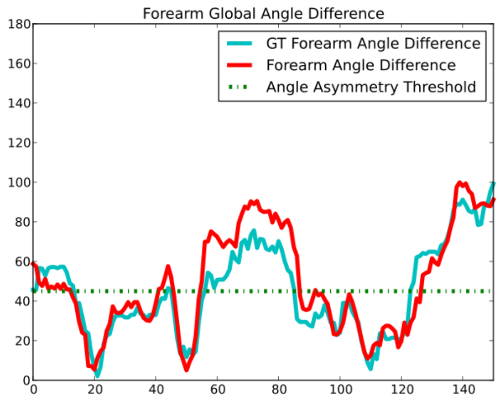
Figures 9-11 present our temporal graphs depicting the asymmetry score , the left and right forearms’ global angles and corresponding difference , as examples for video segments of 4 participants (with ground truth). The forearms’ global angles essentially denote where each one is pointing to w.r.t. the horizontal axis (up, down, horizontally).
In Figure 9a, participant walks asymmetrically holding one forearm in (near) horizontal position pointing sideways, while extending the other arm downwards alongside her body in frames , , and . The graph in this figure represents the asymmetry score computed from both our automatically computed skeleton (red), and the manually created ground truth skeleton (cyan). The asymmetry scores from the automatically computed skeleton and the ones obtained from the ground truth skeleton correlate for this video segment, demonstrating the accuracy of the proposed technique. However, since we compute a 2D skeleton, false positives/negatives might occur due to off-plane rotations (e.g., the false negative indication of asymmetry between frames and ). Figure 9b presents the angle difference measure that might also indicate asymmetry when [18]. By analyzing both and from Figure 9a, one can often rule out false positives/negatives that occur (i.e., the aforementioned false negative indication between frames in Figure 9a is captured by the graph in Figure 9b).
The example in Figure 10a of participant further strenghthens the usage of both and by depicting a false positive indication of asymmetry. Namely, the asymmetry scores between frames denote symmetric behavior for both the ground truth and our automatically computed skeleton, while the scores in Figure 10b indicate false positive asymmetry. Such disagreement occurs because walks with his arms wide open in near frontal view, thereby leading the stickman’s left forearm to appear in horizontal position, while the stickman’s right forearm points vertically down.
Figure 11a depicts the first video segment of participant , in which she walks holding her arms parallel to the ground pointing forward. The graph depicts this behavior by showing the forearm angles w.r.t. the horizontal axis. One can notice the aforementioned stereotypical motor pattern by analyzing from the graph that both forearms are close to the horizontal position for the better part of the video. This shows the array of stereotypical measurements and behaviors we may detect from our body pose estimation algorithm, of which just a few are exemplified here.
Lastly, in Figure 11b participant is not only presenting asymmetric arm behavior throughout the entire video segment, but he is also presenting abnormal gait and hand behavior (other types of stereotypical motor behaviors). We intend to use the skeleton in the detection of such abnormal behaviors as well, by extracting different kinds of measures from it.
For all video sequences, our method presents good average correlation with the ground truth for both , , and , . The correlation of was affected by a negative score of presented for the first video segment of participant , which occurred due to oscilations in our automatically computed skeleton with respect to the ground truth. Nevertheless, the scores computed for both the skeleton and the ground truth denoted symmetry for most of the video segment, agreeing therefore with the clinician’s assessment. If we remove the corresponding video segment, the average increases to (and average to ), indicating high correlation. To correlate our results with the clinician’s categorical assessment of each video segment in Table 2, we threshold SS and DS in and deem a video segment asymmetric when both and . We select such value considering that the average SS for both autistic and non-autistic children was at least in [10], while the average DS was at least . Our method agrees with the clinician’s categorical assessment in out of cases, after excluding video segment 2 of participant since it is abnormal, with non-weighted Cohen’s kappa inter-rater reliability score of (high).
While our method agrees with the clinician’s visual ratings about symmetry for several cases, the expert’s assessment is based on significantly more data. We therefore seek and achieve correlation between our results and the ground truth skeleton to aid in research and diagnosis by complementing human judgement. We have further hypothesized that our body pose estimation algorithm can be used to detect other potentially stereotypical motor behaviors in the future, such as when the toddler is holding his/her forearms parallel to the ground pointing forward. Note that the behaviors here analyzed have only considered simple measures obtained from the skeleton, whereas we can in the future apply pattern classification techniques, in particular when big data is obtained, to achieve greater discriminative power.



6 Conclusion
We have developed an extension of the Cloud System Model framework to do semi-automatic 2D human body segmentation in video. For such purpose, we have coupled the CSM with a relational model in the form of a stickman connecting the clouds in the system, to handle the articulated nature of the human body, whose parameters are optimized using multi-scale search. As a result, our method performs simultaneous segmentation and 2D pose estimation of humans in video.
This work is further inserted in a long-term project for the early observation of children in order to aid in diagnosis of neurodevelopmental disorders [18, 19, 14]. With the goal of aiding and augmenting the visual analysis capabilities in evaluation and developmental monitoring of ASD, we have used our semi-automatic tool to observe a specific motor behavior from videos of in-clinic ASD assessment. Namely, the presence of arm asymmetry in unsupported gait, a possible risk sign of autism. Our tool significantly reduces the effort to only requiring interactive initialization in a single frame, being able to automatically estimate pose and arm asymmetry in the remainder of the video. Our method achieves high accuracy and presents clinically satisfactory results.
We plan on extending the CSM to incorporate full 3D information using a richer 3D kinematic human model [31]. Of course, there are additional behavioral red flags of ASD we aim at addressing. An interesting future direction would be to use our symmetry measurements to identify real complex motor mannerisms from more typical toddler movements.66 6 Bilateral and synchronized arm flapping is common in toddlers as they begin to babble, being hard to judge whether this is part of normal development or an unusual behavior. This issue clearly applies to ’s and ’s clips from their 12-month assessments. This extension also includes detecting ASD risk in ordinary classroom and home environments, a challenging task for which the developments here presented are a first step.
7 Acknowledgments
We acknowledge Jordan Hashemi from the University of Minnesota, for his contributions to the clinical aspect of this work. Work supported by CAPES (BEX 1018/11-6), FAPESP (2011/01434-9 & 2007/52015-0), CNPq (303673/2010-9), NSF Grants 1039741 & 1028076, and the U.S. Department of Defense.
References
- [1] {binproceedings}[author] Bai, XueX., Wang, JueJ. and Sapiro, GuillermoG. (2010). Dynamic Color Flow: A Motion-Adaptive Color Model for Object Segmentation in Video. In ECCV. \endbibitem
- [2] [author] Bai, XueX., Wang, JueJ., Simons, DavidD. and Sapiro, GuillermoG. (2009). Video SnapCut: robust video object cutout using localized classifiers. ACM Trans. Graph. 28 70:1–70:11. \endbibitem
- [3] [author] Boykov, Y.Y. and Funka-Lea, G.G. (2006). Graph Cuts and Efficient N-D Image Segmentation. Int. J. Comput. Vis. 70 109–131. http://dx.doi.org/10.1007/s11263-006-7934-5 \endbibitem
- [4] [author] Chiachia, GiovaniG., Falcão, Alexandre XavierA. X. and Rocha, AndersonA. (2011). Multiscale Parameter Search (MSPS): a Deterministic Approach for Black-box Global Optimization Technical Report No. IC-11-15, IC, University of Campinas. \endbibitem
- [5] [author] Ciesielski, Krzysztof ChrisK. C., Udupa, Jayaram K.J. K., Falcão, A. X.A. X. and Miranda, P. A. V.P. A. V. (2012). Fuzzy Connectedness Image Segmentation in Graph Cut Formulation: A Linear-Time Algorithm and a Comparative Analysis. J. Math. Imaging Vis. 44 375-398. 10.1007/s10851-012-0333-3 \endbibitem
- [6] [author] Cootes, T.T., Taylor, C.C., Cooper, D.D. and Graham, J.J. (1995). Active shape models – their training and application. Comput. Vis. Image Und. 61 38–59. \endbibitem
- [7] [author] Couprie, C.C., Grady, L.L., Najman, L.L. and Talbot, H.H. (2011). Power Watershed: A Unifying Graph-Based Optimization Framework. IEEE Trans. Pattern. Anal. Mach. Intell. 33 1384-1399. \endbibitem
- [8] [author] Dawson, GeraldineG. (2008). Early behavioral intervention, brain plasticity, and the prevention of autism spectrum disorder. Dev. Psychopathol. 20 775–803. \endbibitem
- [9] [author] Eichner, M.M., Marin-Jimenez, M.M., Zisserman, A.A. and Ferrari, V.V. (2012). 2D Articulated Human Pose Estimation and Retrieval in (Almost) Unconstrained Still Images. Int. J. Comput. Vis. 99 190-214. \endbibitem
- [10] [author] Esposito, G.G., Venuti, P.P., Apicella, F.F. and Muratori, F.F. (2011). Analysis of unsupported gait in toddlers with autism. Brain Dev. 33 367–373. \endbibitem
- [11] [author] Falcão, A. X.A. X., Costa, L. F.L. F. and Cunha, B. S.B. S. (2002). Multiscale skeletons by image foresting transform and its application to neuromorphometry. Pattern Recognition 35 1571–1582. \endbibitem
- [12] [author] Falcão, A. X.A. X., Stolfi, J.J. and Lotufo, R. A.R. A. (2004). The Image Foresting Transform: theory, Algorithms, and Applications. IEEE Trans. Pattern. Anal. Mach. Intell. 26(1) 19–29. \endbibitem
- [13] [author] Falcão, A. X.A. X., Udupa, J. K.J. K., Samarasekera, S.S., Sharma, S.S., Hirsch, B. E.B. E. and Lotufo, R. A.R. A. (1998). User-steered image segmentation paradigms: Live-wire and live-lane. Graph. Model. Im. Proc. 60 233-260. \endbibitem
- [14] {binproceedings}[author] Fasching, JoshuaJ., Walczak, NicholasN., Sivalingam, RavishankarR., Cullen, KathrynK., Murphy, BarbaraB., Sapiro, GuillermoG., Morellas, VassiliosV. and Papanikolopoulos, NikolaosN. (2012). Detecting Risk-markers in Children in a Preschool Classroom. In IROS. \endbibitem
- [15] [author] Goodwin, Matthew S.M. S., Intille, Stephen S.S. S., Albinali, FahdF. and Velicer, Wayne F.W. F. (2011). Automated Detection of Stereotypical Motor Movements. J. Autism Dev. Disord. 41 770–782. \endbibitem
- [16] [author] Grady, L.L. (2006). Random Walks for Image Segmentation. IEEE Trans. Pattern. Anal. Mach. Intell. 28 1768–1783. \endbibitem
- [17] {binproceedings}[author] Grundmann, MatthiasM., Kwatra, VivekV., Han, MeiM. and Essa, IrfanI. (2010). Efficient Hierarchical Graph Based Video Segmentation. In CVPR. \endbibitem
- [18] {binproceedings}[author] Hashemi, JordanJ., Spina, Thiago V.T. V., Tepper, MarianoM., Esler, AmyA., Morellas, VassiliosV., Papanikolopoulos, NikolaosN. and Sapiro, GuillermoG. (2012). A computer vision approach for the assessment of autism-related behavioral markers. In ICDL-EpiRob. \endbibitem
- [19] [author] Hashemi, JordanJ., Spina, Thiago VallinT. V., Tepper, MarianoM., Esler, AmyA., Morellas, VassiliosV., Papanikolopoulos, NikolaosN. and Sapiro, GuillermoG. (2012). Computer vision tools for the non-invasive assessment of autism-related behavioral markers. CoRR abs/1210.7014. \endbibitem
- [20] {binproceedings}[author] Ionescu, C.C., Li, FuxinF. and Sminchisescu, C.C. (2011). Latent structured models for human pose estimation. In ICCV. \endbibitem
- [21] [author] Kohli, PushmeetP., Rihan, JonathanJ., Bray, MatthieuM. and Torr, PhilipP. (2008). Simultaneous Segmentation and Pose Estimation of Humans Using Dynamic Graph Cuts. Int. J. Comput. Vis. 79 285-298. \endbibitem
- [22] [author] Liu, JiaminJ. and Udupa, J. K.J. K. (2009). Oriented Active Shape Models. IEEE Trans. Med. Imaging 28 571-584. 10.1109/TMI.2008.2007820 \endbibitem
- [23] [author] Minetto, R.R., Spina, T. V.T. V., Falcão, A. X.A. X., Leite, N. J.N. J., Papa, J. P.J. P. and Stolfi, J.J. (2012). IFTrace: Video segmentation of deformable objects using the Image Foresting Transform. Comput. Vis. Image Underst. 116 274–291. \endbibitem
- [24] {binproceedings}[author] Miranda, Paulo A. V.P. A. V., Falcão, Alexandre X.A. X. and Udupa, Jayaram K.J. K. (2009). Cloud bank: a multiple clouds model and its use in MR brain image segmentation. In ISBI. \endbibitem
- [25] [author] Miranda, P. A. V.P. A. V. and Falcão, A. X.A. X. (2009). Links Between Image Segmentation Based on Optimum-Path Forest and Minimum Cut in Graph. J. Math. Imaging Vis. 35 128–142. \endbibitem
- [26] [author] Miranda, Paulo A. V.P. A. V., Falcão, Alexandre X.A. X. and Udupa, Jayaram K.J. K. (2010). Cloud Models: Their Construction and Employment in Automatic MRI Segmentation of the Brain Technical Report No. IC-10-08, IC, University of Campinas. \endbibitem
- [27] {binproceedings}[author] Nazneen, FnuF., Boujarwah, Fatima A.F. A., Sadler, ShoneS., Mogus, AmhaA., Abowd, Gregory D.G. D. and Arriaga, Rosa I.R. I. (2010). Understanding the challenges and opportunities for richer descriptions of stereotypical behaviors of children with ASD: a concept exploration and validation. In ACM SIGACCESS. ASSETS. \endbibitem
- [28] {binproceedings}[author] Ochs, P.P. and Brox, T.T. (2011). Object segmentation in video: a hierarchical variational approach for turning point trajectories into dense regions. In ICCV. \endbibitem
- [29] {binproceedings}[author] Price, Brian L.B. L., Morse, Bryan S.B. S. and Cohen, ScottS. (2009). LIVEcut: Learning-based interactive video segmentation by evaluation of multiple propagated cues. In ICCV. \endbibitem
- [30] [author] Shattuck, Paul T.P. T., Durkin, MaureenM., Maenner, MatthewM., Newschaffer, CraigC., Mandell, David S.D. S., Wiggins, LisaL., Lee, Li-Ching C.L.-C. C., Rice, CatherineC., Giarelli, EllenE., Kirby, RussellR., Baio, JonJ., Pinto-Martin, JenniferJ. and Cuniff, ChristopherC. (2009). Timing of identification among children with an autism spectrum disorder: findings from a population-based surveillance study. J. Am. Acad. Child Adolesc. Psychiatry 48 474–483. \endbibitem
- [31] [author] Sherman, Michael A.M. A., Seth, AjayA. and Delp, Scott L.S. L. (2011). Simbody: multibody dynamics for biomedical research. Procedia IUTAM 2 241 - 261. \endbibitem
- [32] {binproceedings}[author] Sivalingam, R.R., Somasundaram, G.G., Bhatawadekar, V.V., Morellas, V.V. and Papanikolopoulos, N.N. (2012). Sparse representation of point trajectories for action classification. In ICRA. \endbibitem
- [33] {binproceedings}[author] Spina, Thiago VallinT. V., Falcão, Alexandre XavierA. X. and Miranda, Paulo André VechiattoP. A. V. (2011). User-steered image segmentation using live markers. In CAIP. \endbibitem
- [34] [author] Teitelbaum, OsnatO., Benton, TomT., Shah, Prithvi K.P. K., Prince, AndreaA., Kelly, Joseph L.J. L. and Teitelbaum, PhilipP. (2004). Eshkol-Wachman movement notation in diagnosis: The early detection of Asperger ’s syndrome. Proc. Natl. Acad. Sci. USA 101 11909–11914. \endbibitem
- [35] {binproceedings}[author] Tepper, M.M. and Sapiro, G.G. (2012). Decoupled coarse-to-fine matching and nonlinear regularization for efficient motion estimation. In ICIP. \endbibitem
- [36] {binproceedings}[author] Udupa, Jayaram K.J. K., Odhner, DeweyD., Falcão, Alexandre X.A. X., Ciesielski, Krzysztof C.K. C., Miranda, Paulo A. V.P. A. V., Matsumoto, MonicaM., Grevera, George J.G. J., Saboury, BabakB. and Torigian, Drew A.D. A. (2012). Automatic anatomy recognition via fuzzy object models. In SPIE Medical Imaging. 10.1117/12.911580 \endbibitem
- [37] {binproceedings}[author] Udupa, Jayaram K.J. K., Odhner, DeweyD., Falcão, Alexandre X.A. X., Ciesielski, Krzysztof C.K. C., Miranda, Paulo A. V.P. A. V., Vaideeswaran, PavithraP., Mishra, ShipraS., Grevera, George J.G. J., Saboury, BabakB. and Torigian, Drew A.D. A. (2011). Fuzzy object modeling. In SPIE Medical Imaging. \endbibitem
- [38] [author] Udupa, J. K.J. K., Saha, P. K.P. K. and Lotufo, R. A.R. A. (2002). Relative Fuzzy Connectedness and Object Definition: Theory, Algorithms, and Applications in Image Segmentation. IEEE Trans. Pattern. Anal. Mach. Intell. 24 1485–1500. \endbibitem
- [39] {binproceedings}[author] Yao, BangpengB. and Fei-Fei, LiL. (2012). Action Recognition with Exemplar Based 2.5D Graph Matching. In ECCV. \endbibitem
- [40] {binproceedings}[author] Zuffi, S.S., Freifeld, O.O. and Black, M. J.M. J. (2012). From pictorial structures to deformable structures. In CVPR. \endbibitem