On the Coloring of Pseudoknots
Abstract
Pseudodiagrams are diagrams of knots where some information about which strand goes over/under at certain crossings may be missing. Pseudoknots are equivalence classes of pseudodiagrams, with equivalence defined by a class of Reidemeister-type moves. In this paper, we introduce two natural extensions of classical knot colorability to this broader class of knot-like objects. We use these definitions to define the determinant of a pseudoknot (i.e. the pseudodeterminant) that agrees with the classical determinant for classical knots. Moreover, we extend Conway notation to pseudoknots to facilitate the investigation of families of pseudoknots and links. The general formulae for pseudodeterminants of pseudoknot families may then be used as a criterion for -colorability of pseudoknots.
1 Introduction
1.1 Pseudodiagrams and pseudoknots
Recently, Ryo Hanaki introduced the notion of a pseudodiagram of a knot, link, and spatial graph [6]. A pseudodiagram of a knot or link is a knot or link diagram that may be missing some crossing information, as in Figure 1. In other words, at some crossings in a pseudodiagram, it is unknown which strand passes over and which passes under. These undetermined crossings are called precrossings and are pictured simply as self-intersections. Special classes of pseudodiagrams are knot diagrams and knot shadows, i.e. pseudodiagrams containing only precrossings. Pseudodiagrams were originally considered because of their potential to serve as useful models for biological objects related to DNA, but they are interesting objects in their own right. Pseudodiagrams and their virtual counterparts have also been studied in [5].

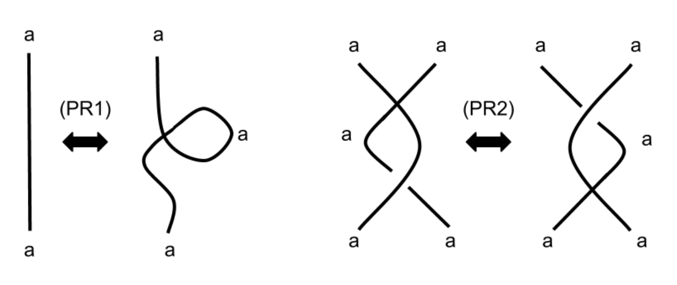
In [4], the idea of pseudodiagrams is extended to pseudoknots (and pseudolinks), i.e. equivalence classes of pseudodiagrams modulo pseudo-Reidemeister moves (shown in Figure 2). The primary invariant explored in [4] is the WeRe-set (Weighted Resolution set) of a pseudoknot. The WeRe-set of a pseudoknot is the set of ordered pairs where the first entry of a pair is a knot that may be realized by resolving all crossings in a pseudodiagram of the pseudoknot, and the second entry is the probability of obtaining the given knot type in a random resolution of precrossings. While the WeRe-set is a powerful invariant, it may be difficult to compute for pseudoknots with large precrossing numbers. Thus, our aim is to expand the number of tools that can be used for classification of pseudoknots. One natural invariant to consider, pseudoknot colorability, is the subject of this paper.

1.2 Knot colorability
For knots, a -coloring of a diagram is an assignment of elements of to arcs in the diagram such that at each crossing, two times the element assigned to the over-arc equals the sum of the elements assigned to the under-arcs. It can easily be shown that if one diagram of a knot has a non-trivial -coloring, then so does every other diagram of the knot. We say that a knot is -colorable (or colorable mod ) if there exists a non-trivial -coloring of each of its diagrams.
If , we note that the coloring condition for the crossings is satisfied if and only if the three arcs that meet at a crossing are either colored with all different “colors” (that is, elements of ) or all the same color.
In general, to determine for which a given knot is -colorable, we begin by fixing a diagram of the knot. In , we assign a variable to each arc and write an equation of the form for every crossing, where and represent the variables assigned to the under-arcs and represents the variable assigned to the over-arc. We obtain in this way a system of equations in variables, where is the crossing number of the diagram (which is also equal to the number of arcs in the diagram). Forming a matrix corresponding to this system, we say the determinant of the knot is the determinant of any submatrix (which is independent of the particular submatrix chosen). The knot given by diagram , then, is -colorable if and only if divides this determinant.
1.3 Pseudoknot colorability
There are two extensions of the classical notion of -colorability we’d like to explore in this paper. One notion we refer to as strong -colorability, and a weaker notion we will simply refer to as -colorability. First, let us be clear that arcs in a pseduodiagram begin and end at classical crossings only. In other words, arcs may merely pass through precrossings.
Definition 1
A pseudodiagram is strong -colorable (or strong colorable mod ) if the arcs of the diagram can be “colored” (i.e. labelled) with elements of , subject to the following conditions.
- 1.
Given a classical crossing, two times the element assigned to the over-arc is equal to the sum of the elements assigned to the under-arcs, mod .
- 2.
For each precrossing , there is a neighborhood of and an element such that all arcs of the diagram in the neighborhood are colored with .
In Section 3, we show that this notion of colorability is a pseudoknot invariant. We also explore the following notion of colorability. Two pseudoknots are said to be -colorable (or colorable mod ) if all of its resolutions are -colorable classical knots. This, too is an invariant. It is not difficult to see that if a pseudoknot is strong -colorable, then it is -colorable. We use -colorability for pseudoknots to define the pseudodeterminant of a pseudoknot.
Before we discuss colorability further in Section 3, we begin the body of our paper in Section 2 by providing background on Conway notation for classical knots and extending this notation to pseudoknots. This will facilitate our discussion of the colorability of families of pseudoknots in Section 4.
2 Conway notation for classical and pseudoknots
2.1 Classical Conway notation
All classical knots and links (or shortly s) can be described using Conway notation. For readers unfamiliar with the conventions, we describe Conway notation as it was introduced in Conway’s seminal paper [2] published in 1967, and effectively used since (e.g., [12, 1, 9]). Conway symbols of knots with up to crossings and links with at most crossings are given in the Appendix of the book [12].

The main building blocks in the Conway notation are elementary tangles. We distinguish three elementary tangles, shown in Fig. 3. These are commonly denoted by 0, 1, and . All other tangles can be obtained by combining elementary tangles, while 0 and 1 are sufficient for generating alternating s. Elementary tangles can be combined by the following three operations: sum, product, and ramification (Figs. 4-5). Given tangles and , we denote by the image of under reflection about the line joining the Northwest and Southeast corners of a the tangle diagram. The sum of and is denoted by , while the product is defined as . Furthermore, the binary operation ramification is given by .


A tangle can be closed in two ways without introducing additional crossings. We can join the pairs of ends at the Northeast and Northwest corners of the tangle diagram as well as the Southeast and Southwest ends of the tangle to obtain the numerator closure. The closure obtained by joining the Northeast and Southeast ends as well as the Northwest and Southwest ends is called the denominator closure (Fig. 6a,b).

Definition 2
A rational tangle is any tangle that is equivalent to a finite product of elementary tangles. A rational is a knot or link that can be obtained by taking the numerator closure of a rational tangle.
Definition 3
A tangle is algebraic if it can be obtained from elementary tangles using the operations of sum and product. An algebraic is a knot or link that can be obtained by taking the numerator closure of an algebraic tangle.
Example 1
A Montesinos tangle and the corresponding Montesinos consist of alternating rational tangles , including at least three non-elementary tangles for . (See Fig. 7.) We denote a Montesinos link by , where . The number of tangles, , is called the length of the Montesinos tangle.
If all tangles for are integer tangles (i.e. tangles of the form or ), where , we obtain pretzel s.

Definition 4
A basic polyhedron is a -regular, -edge-connected, at least -vertex connected plane graph.
A basic polyhedron [2, 12, 1, 9] of a given can be identified by recursively collapsing all bigons in a diagram, until no bigons remain 8.

Definition 5
A link is algebraic or a -link if there exists at least one diagram of which can be reduced to the basic polyhedron by a finite sequence of bigon collapses. Otherwise, it is a non-algebraic or polyhedral link.
Conway notation for polyhedral s begins with the symbol denoting a basic polyhedron (together with a standard ordering of its vertices). The symbol (where is the shorthand for a sequence of stars) denotes the -th basic polyhedron in the list of basic polyhedra with vertices. A obtained from the basic polyhedron by substituting the first vertices with tangles , , , where is denoted by . A common shorthand convention allows us to replace a substituent of value 1 by a colon. If , we replace each of the vertices by the elementary tangle 1. Let us illustrate how this notation works with some examples. The notation is shorthand for , and is shorthand for Both examples are pictured in Fig. 9.

We now recall a useful technique for defining a family of s from a particular knot or link.
Definition 6
For a knot or link, , given using unreduced11 1 The Conway notation is called unreduced if the 1’s that denote replacing vertices by the elementary tangle 1 are not omitted. E.g. rather than . Conway notation , denote by the set of numbers in the Conway symbol, where numbers denoting basic polyhedra and zeros (determining the position of tangles in the vertices of polyhedron) are excluded. Let be a non-empty subset of . The family of s derived from consists of all knots or links whose Conway symbol is obtained by substituting all , by , , where .
An infinite subset of a family of s is called subfamily. Note that if all are even integers, the number of components is preserved within the corresponding subfamilies, i.e., adding full-twists preserves the number of components inside the subfamilies.
Definition 7
A link given by a Conway symbol containing only tangles and is called a source link. A link given by a Conway symbol containing only tangles , , or is called a generating link.
For example, the Hopf link, , (which is link in Rolfsen’s notation) is the source link of the simplest link family, , () shown in Fig. 10. The Hopf link and the trefoil, , (knot in the classical notation) are generating links of this family. A family of s is usually derived from its source link by substituting , where , by , (see Def. 5 and Def. 6).

2.2 Conway notation for pseudoknots and links
Analogous to the Conway notation for classical s we use extended Conway notation for pseudodiagrams and pseudolinks, by adding to the list of the elementary tangles , , the elementary tangle denoting a precrossing. To be clear, the extended Conway notation for pseudoknots differs from the standard one in the following way:
- •
pseudocrossings are denoted by .
- •
sequence of classical crossings (positive -twist) is denoted by
- •
sequence of classical negative crossings (negative -twist) is denoted by
The convention introduced in the Conway notation extended to pseudodiagrams is natural, given that every positive -twist can be denoted by , and every negative -twist by This convention extends to pseudoknot families. For example, consider the simplest family , , , , of knots and links, generated by the Hopf link, , and the trefoil, , where the family member with crossings is denoted by , as described above. We generate a family of pseudoknots and links by substituting a crossing in each member of the family by a precrossing, we obtain the family of pseudoknots and pseudolinks , , , , , and in general for (Fig. 11).

3 Colorability of pseudoknots
We now return to our study of coloring invariants. In our introduction, we defined two notions of colorability for pseudoknots: strong -colorability and -colorability. We prove that these notions both yield pseudoknot invariants.
Theorem 1
Strong -colorability is an invariant of pseudoknots.
Proof. Because -colorability is an invariant of classical knots and strong -colorability for classical pseudoknots is equivalent to ordinary -colorability for classical knots, we can be sure that the classical Reidemeister moves preserve strong -colorability. Let us, then, consider the pseudo-Reidemeister (PR) moves.
First we note that the PR1 move preserves strong -colorability, for the arcs involved in the move must be colored by the same element. This is simply due to the fact that arcs cannot begin and end at a precrossing.
Considering the PR2 move, all but one arc involved in the move is forced by the precrossing condition to be colored with a single element. Thus, the remaining arc must be colored with the same element (since is the only solution to ), regardless of whether we are considering the local picture before or after the move has been performed. See Figure 12.
The PR3 and PR moves are somewhat more complicated. Consider the PR3 move where the free strand passes under the precrossing. The arcs passing through the precrossing must be the colored with the same element (let’s call it ), but the remaining arcs may be colored differently. Consider the central arc (i.e. the one labeled with a in the bottom left corner of Figure 12). Regardless of whether or not differs from , the remaining two arcs must be colored with (in particular, in the case that ). This coloring uniquely determines the valid coloring of the local picture after the PR3 move has been performed.
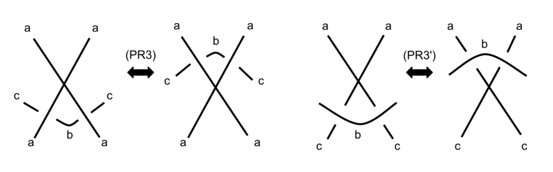
Consider the PR move pictured in Figure 12. On the left, the top two arcs are forced by the precrossing to be colored by the same element, . We color the over-arc with element , which may or may not equal . Then both remaining arcs are colored with . Since both of the remaining arcs must be colored with the same element, we see that the induced coloring on the local picture after the move has been performed (pictured on the right) includes a valid coloring of the precrossing.
Let’s look at an example. According to Definition 1, the pseudodiagram will not be strong 3-colorable. This is because, in every coloring of diagram mod 3, all three colors appear in every crossing, so there is no coloring mod 3 of this pseudodiagram where only one color appears in a neighborhood of the precrossing. However, if we consider the weaker notion of -colorability in Definition 8, our example will be colorable mod 3. Indeed, both of its resolutions, and , are colorable mod 3 in the classical sense (Fig. 13). The existence of examples of this sort, prompts us to explore further the notion of colorability mod for pseudoknots. Let us recall our definition.
Definition 8
A pseudoknot is -colorable (or colorable mod ) if all of its resolutions are colorable mod .

Theorem 2
Colorability mod is an invariant of pseudoknots.
Proof. Suppose that a pseudodiagram is colorable mod , and let be one of its resolutions. (So is a knot diagram that is colorable mod .) Suppose a (classical) Reidemeister move is applied to to produce a new diagram , and apply the corresponding Reidemeister move to to obtain the diagram . Note that is a resolution of , and since mod colorability is an invariant of classical knots, remains mod colorable. Thus, is mod colorable.
Suppose, instead, that a non-classical pseudo-Reidemeister (PR) move is applied to to produce . If the move applied is the PR1 move that introduces a new precrossing, then there are two new resolutions of that are each related to by a Reidemeister 1 move. (One move introduces a positive kink in and one introduces a negative kink.) These two resolutions are colorable mod since is. If the move applied is the PR1 move that reduces the number of crossings by one, then a simple R1 move may be applied to to get the corresponding resolution of . Again, this resolution will be colorable mod since is. If a PR2, PR3, or PR3’ move is applied to , there is a unique corresponding Reidemeister 2 or 3 move that may be applied to to obtain a resolution, of . (Note that the proof of this statement is similar to the proof of invariance of the WeRe-set in [4].) Thus is also colorable mod . Hence, is colorable mod .
Example 2
Pseudoknots and (Fig. 14) are -colorable for .


Definition 9
A pseudodiagram obtained from another pseudodiagram with precrossings () by resolving at most of its precrossings will be called a pseudoresolution of .
Proposition 3
If a pseudodiagram containing precrossings is colorable mod , then all of its pseudoresolutions are colorable mod .


For every pseudoknot, we can define its coloring numbers to be the set of numbers for which it is colorable mod . For example, pseudoknot is colorable mod 3, mod 5, and mod 15 (Fig. 19). We see that the coloring numbers of a pseudoknot can be determined from ’s resolution set using the following notion.


Definition 10
Let be a pseudoknot with resolution set , , . Then
is called the pseudodeterminant of .
Note that, for classical knots, the notion of the pseudodeterminant coincides with the definition of the determinant of a knot. Also from this definition, we immediately have the following proposition, as illustrated in Fig. 20.
Proposition 4
If , , are all resolutions of , then will be colorable mod for every which divides its pseudodeterminant.
We can use the notion of a pseudodeterminant to learn about the colorability of families of knots. Many families of knots given in Conway notation can be described using pseudotwists.
Definition 11
A pseudotwist is a twist of length which contains at least one precrossing.
Note that if a pseudotwist of length in a link pseudodiagram is replaced by a pseudotwist with length where is an integer, then the number of components of the pseudolink is preserved. Performing the operation of replacing twists, we obtain families of pseudoknots and pseudolinks. In every family, a pseudotwist can be replaced by pseudotwist , () in order to obtain all of its pseudoresolutions.
Theorem 5
Suppose is the diagram of a pseudolink that contains at least one pseudotwist. Then any link pseudodiagram obtained from by replacing a pseudotwist in with a pseudotwist that has a length of the same parity will have the same pseudodeterminant.
Before we prove Theroem 5, let us make some general remarks about the behavior of knot determinants. Suppose we have a link given in Conway notation that contains a twist of length , where is an integer. Let’s call this link . Now suppose we replace the length twist with a length twist for some integer to obtain . If we let , then there exists an such that for all , . See [11] for more details. We make use of this result in the following proof.
Proof. Let be the diagram of a pseudolink that contains only one simple pseudotwist . Denote the determinants of the resolutions of this precrossing by and (), and let denote the pseudodeterminant of . Let be the pseudodiagram obtained from by replacing by another pseudotwist of odd length. In order to prove that the pseudodeterminant of equals that of , we first show as a base case that the pseudodeterminant remains unchanged if we replace by a pseudotwist of length three.
Notice that the pseudodeterminant remains unchanged by any permutation of crossings in a pseudotwist (since any permutation of crossings is equivalent to the original ordering by some sequence of PR2 moves). If we replace the pseudotwist in by , it is clear that pseudodeterminant remains unchanged, since the two tangles are related by a R2 move. If, on the other hand, we replace by , , , , or , the pseudodeterminants of the resulting pseudolinks will be , , , , or , respectively.
To see why, consider the last example where is replaced by . We claim that the determinant of this pseudoknot is . If two precrossings in are resolved to be positive and one negative, the resulting link contains the twist in its Conway notation and there are three ways to choose where the negative crossing occurs. Similarly, if two precrossings in are resolved to be negative and one positive, the resulting link contains the twist in its Conway notation and there are three ways to choose where the positive crossing occurs. This accounts for the terms and each repeated three times. The determinants and correspond to a choice of all positive or all negative crossings.
In each case of replacing by a length three pseudotwist, the pseudodeterminant remains unchanged. The induction step is proven similarly since is a subtwist of any pseudotwist. Therefore, in may be replaced by any odd-length pseudotwist to produce a pseudolink with the same pseudodeterminant as .
The inductive proof for the even length pseudotwist is similar. Indeed, since is a subtwist of every pseudotwist, any pseudotwist (regardless of the parity of its length) can be replaced by any other pseudotwist with length of the same parity without changing the pseudodeterminant.
For example, consider the family of pseudoknots comprised of together with all of the pseudoknots obtained by replacing the pseudotwists and each by arbitrary pseudotwists of the same parity. Each pseudoknot in this family has pseudodeterminant 9 since, for instance, , by Theorem 5.
Remark 4
Computing the coloring numbers of pseudoknots with crossings, we find evidence that a very small portion of pseudoknots will be non-trivially colorable: from 8583 knots with crossings, only 112 will be non-trivially colorable, 70 with , 11 with , 5 with , 23 with , 1 with , 1 with , and 1 with .
4 Families of Pseudoknots and Conjectures
4.1 Pseudoknot families and their colorings
Instead of considering particular pseudoknots and their colorings, we may explore the extension of colorability to families of pseudoknots (given in Conway notation). Take, for example, the pseudoknot with . This pseudoknot is the first member of the family of pseudoknots which contains nontrivially colorable pseudoknots. All resolutions of are rational knots of the form , with , , and , with determinant
for every . (See [11] for more on computing determinants of rational knots.) The of these determinants, i.e., the pseudodeterminant, will be . For example, pseudoknots have , while pseudoknots have , etc.
In Appendix A, we provide a table of families of colorable pseudoknots that are derived from pseudoknots with at most crossings. In the same way as for the example above (which is entry (1) in our table), we can obtain general formulae for the pseudodeterminant of pseudoknot families by using general formulae for the determinants of classical knots. For example, for family (2) from the table, the determinant is
for every , so the pseudodeterminant is . Knowing that the determinant of classical rational knots and links is given by the general formula
for every , we also conclude that for family (3), the pseudodeterminant is again . Proceeding in this way, we determine all entries in the table.
4.2 The Kauffman-Harary Conjecture
A knot diagram is said to have the Kauffman-Harary property (or KH property for short) if it can be endowed with a nontrivial coloring mod which assigns a unique color to each arc [7]. A pseudodiagram is said to have the KH property if all of its resolutions have the KH property. The smallest example of a pseudodiagram with the KH property is the pseudodiagram . Both of its resolution diagrams and have the KH property for the coloring mod 9 (Fig. 21). The KH property is not just a property of particular pseudoknots, but of the entire families. For example, all pseudoknots with have KH property. Indeed, we find that both resolution diagrams and are colorable mod with different colors. Figure 22 shows the second member of this family, pseudoknot with and its resolution diagrams and colored mod 25 with 11 colors.


Another example of a pseudoknot family with the KH property is the family with . Both of its resolution diagrams and are colorable mod with colors (Fig. 23). This family can be extended to the pseudoknot family with the KH property, where , and each diagram is colorable mod with colors (Fig. 24).
An interesting question involving the KH property for pseudoknots relates to the idea of a pseudoalternating pseudodiagram. A pseudodiagram is pseudoalternating if it has an alternating resolution.
Conjecture 1
A pseudodiagram with the KH property cannot be pseudoalternating.
We conclude our exploration of pseudoknot colorability with another idea concerning a possible direction for future work. More open problems about colorings of pseudoknots relate to the number of colors used for coloring mod . For every pseudoknot colorable mod , we can define and as the minimal and maximal number of colors needed for coloring , where both numbers are taken over all diagrams of [10]. Just as in the case of classical knots, the first invariant will be very hard to compute. This is because, for every knot with and , there exists a diagram that is colorable using colors, where . In other words, the coloring spectrum of every knot is the complete set [10]. The same holds for pseudoknots. For a pseudoknot , will be the maximum of minimal coloring numbers of its resolutions, and is equal to pseudodeterminant of .
Appendix A Pseudoknot Tables
In this section, we provide a table of pseudoknot families together with their pseudodeterminants.
| 1) | ||
|---|---|---|
| 2) | ||
| 3) | ||
| 4) | ||
| 5) | ||
| 6) | ||
| 7) | ||
| 8) | ||
| 9) | ||
| 10) | ||
| 11) | ||
| 12) | ||
| 13) | ||
| 14) | ||
| 15) | ||
| 16) | ||
| 17) | 3 | |
| 18) | 3 | |
| 19) | 3 | |
| 20) | ||
| 21) | ||
| 22) | ||
| 23) | ||
| 24) | ||
| 25) | ||
| 26) | ||
| 27) | ||
| 28) | ||
| 29) | ||
| 30) |
| 31) | ||
|---|---|---|
| 32) | ||
| 33) | 3 | |
| 34) | 3 | |
| 35) | 9 | |
| 36) | 9 | |
| 37) | ||
| 38) | ||
| 39) | ||
| 40) | ||
| 41) | ||
| 42) | ||
| 43) | ||
| 44) | ||
| 45) | ||
| 46) | ||
| 47) | 5 | |
| 48) | 5 | |
| 49) | 5 | |
| 50) | 3 | |
| 51) | 3 | |
| 52) | 3 | |
| 53) | 3 | |
| 54) | 9 | |
| 55) | 9 | |
| 56) | 9 | |
| 57) | 9 | |
| 58) | ||
| 59) | ||
| 60) |
References
- [1] A. Caudron, Classification des nœuds et des enlancements, Public. Math. d’Orsay 82. Univ. Paris Sud, Dept. Math., Orsay, 1982.
- [2] J. Conway, An enumeration of knots and links and some of their related properties, in Computational Problems in Abstract Algebra, Proc. Conf. Oxford 1967 (Ed. J. Leech), 329–358, Pergamon Press, New York (1970).
- [3] R.H. Crowell, Genus of alternating link types, Ann. of Math. 69 (1959), 258–275.
- [4] A. Henrich, R. Hoberg, S. Jablan, L. Johnson, E. Minten, Lj. Radović, The Theory of Pseudoknots, arXiv:1210.6934v2 [math.GT]
- [5] A. Henrich, N. MacNaughton, S. Narayan, O. Pechenik, and J. Townsend. Classical and virtual pseudodiagram theory and new bounds on unknotting numbers and genus. J. Knot Theory Ramifications, 20 (2011) pp. 625-650.
- [6] R. Hanaki. Pseudo diagrams of knots, links and spatial graphs. Osaka J. Math. 47 (2010), 863-883.
- [7] F. Harary, L. Kauffman, Knots and graphs. I. Arc graphs and colorings, Adv. in Appl. Math. 22 (1999), 3, 312–337
- [8] S. Jablan, Lj. Radović and R. Sazdanović, Tutte and Jones polynomials of link families, Filomat 24, 3 (2010), 19–33 (http://operator.pmf.ni.ac.rs/www/pmf/publikacije/filomat/2010/ F24-3-2010/F24-3-3.pdf), (arXiv:0902.1162v2 [math.GT]).
- [9] S. V. Jablan and R. Sazdanović, LinKnot – Knot Theory by Computer, World Scientific, New Jersey, London, Singapore, 2007; http://math.ict.edu.rs/.
- [10] S. Jablan, L. Kauffman, P. Lopes, On the Maximum Number of Colors for Links, arXiv:1205.1467v2 [math.GT]
- [11] L.H. Kauffman, P. Lopes, Determinants of Rational Knots, Discrete mathematics and Theoretical Computer Science, 11, 2, (2009), 111–122.
- [12] D. Rolfsen, Knots and Links, (Publish & Perish Inc., Berkeley, 1976); American Mathematical Society, AMS Chelsea Publishing, 2003.