Magnetic diffusion effects on the Ultra-High Energy
Cosmic Ray spectrum and composition
Abstract
We discuss the effects of diffusion of high energy cosmic rays in turbulent extra-galactic magnetic fields. We find an approximate expression for the low energy suppression of the spectrum of the different mass components (with charge ) in the case in which this suppression happens at energies below EeV, so that energy losses are dominated by the adiabatic ones. The low energy suppression appears when cosmic rays from the closest sources take a time comparable to the age of the Universe to reach the Earth. This occurs for energies in terms of the magnetic field RMS strength , its coherence length and the typical separation between sources . We apply this to scenarios in which the sources produce a mixed composition and have a relatively low maximum rigidity (– EeV), finding that diffusion has a significant effect on the resulting spectrum, the average mass and on its spread, in particular reducing this last one. For reasonable values of and these effects can help to reproduce the composition trends observed by the Auger Collaboration for source spectra compatible with Fermi acceleration.
1 Introduction
Charged particles traversing a region with a turbulent magnetic field characterized by an RMS strength can be in three different propagation regimes depending on the relation between the magnetic field coherence length , the source distance and the Larmor radius
| (1) |
with the particle charge, and (with eV).
Defining the critical energy such that , one obtains EeV. For energies , one has that so that diffusion occurs through the resonant scattering of the particles on the magnetic field components with wavelengths of order . This propagation regime is usually referred to as the quasi-linear regime or resonant diffusion. The diffusion length depends on the power of the magnetic field on the scales of the Larmor radius, and hence depends on the turbulent magnetic field spectrum. Typically one has , where for a Kolmogorov spectrum , for a Kraichnan spectrum while the so-called Bohm diffusion adopts (corresponding to the assumption ). The diffusion length corresponds to the distance for which the typical particle deflection is 1 rad, and hence is related to the basic step in the random walk of the diffusing particles. The diffusion coefficient is just and the rectilinear distance travelled by particles in their random walk after a time satisfies .
When (i.e. for ) the scattering is non-resonant and is the result of many small deflections, with in each coherence length . As a result, after steps the deflection is rad, so that one obtains and we see that the diffusion length strongly increases with energy. Two regimes are possible here depending on the overall distance travelled (i.e. depending on the source distance ). As long as spatial diffusion of the particles takes place, while at energies for which becomes larger than the overall deflections become small and the quasi-rectilinear propagation of the particles takes place, leading to just a small angular diffusion of the particle trajectories.
Cosmic rays (CRs) arriving to the Earth are deflected by both the galactic and the extra-galactic magnetic fields. Regarding the deflections in the galactic fields, which have typical strengths of few G with the random component having –100 pc, the critical energy is EeV and the particles reach the quasi-rectilinear propagation in the turbulent field ( kpc, which is the typical vertical extent of the random magnetic field) for energies eV, and somewhat larger for directions along the galactic plane. Actually, the dominant deflections in the galactic magnetic field are expected to be those caused by the regular component, due to its larger coherence length of order kpc. As a result, the galactic magnetic field deflections at EeV energies are large even for CR protons. Although these deflections can significantly modify the arrival directions (hence diluting possible anisotropy signals) they do not affect the expected overall spectrum nor the composition of the extra-galactic cosmic rays.
Focusing now on the extra-galactic magnetic fields, the simplest assumption is to consider a uniform turbulent field permeating intergalactic space. Strengths for in the range from 0.01 nG up to 100 nG and coherence lengths from 10 kpc (as could be associated to galactic outflows) up to 50 Mpc (as could be associated to supercluster scales) have been considered11 1 Notice that for a Kolmogorov spectrum with maximum scale of turbulence and minimum one one has that [1]. . For instance the simulations in [2] obtain nG in filaments while –100) nG outside filaments, while ref. [3] obtains values nG in voids and nG in filaments, with fields inside clusters being at the G level. The possible impact on the CR diffusion of non-uniform magnetic fields and of its possible cosmological evolution were discussed in [4]. A review with some magnetic field upper bounds obtained in the literature for different values of can be found in [5].
The average separation between the UHECR sources is related to their density through , with Mpc for Mpc-3 while Mpc for Mpc-3, which covers the range of densities usually considered. CRs from a source at distance will have a diffusive propagation (i.e. ) as long as , where (assuming the non-resonant diffusive regime to hold) one gets
| (2) |
Hence, even protons from the closest sources may have a diffusive behavior up to EeV energies for values of , and up to higher energies for sources farther away, with nuclei having a similar behavior but shifted up in energy by a factor (i.e. equal for the same rigidities).
Two additional ingredients are fundamental in shaping the CR spectra of the different elements: the interactions with the radiation backgrounds and cosmological evolution effects. CR energy losses arise from adiabatic losses (d, with being Hubble’s constant in terms of the scale factor ), which are present at all energies, and from the interaction losses due to different processes. The pair ( creation losses are relevant for interactions with CMB photons of energy eV, requiring CR Lorentz factors and hence EeV for nuclei with mass number . Actually, the energy loss length for protons becomes smaller than the Hubble horizon , with km/s/Mpc, for energies EeV, while for heavy nuclei the combination of increased threshold and larger pair production cross section, , leads to an energy loss length comparable to for EeV [6]. The photo-pion production off CMB photons becomes significant only for very high energies, EeV, while the photo-disintegration of nuclei is relevant for EeV for interactions with CMB photons and down to lower energies for interactions with higher energy background photons such as IR or optical ones. However, for interactions with IR photons the energy loss length for photo-disintegration is larger than the Hubble horizon except for heavy nuclei such as Fe for which it is larger than only for EeV [6]. As a result of these considerations, we can say that in general for EeV the energy losses are mainly due to the adiabatic ones while the ones due to interactions are small.
In addition to the adiabatic losses, cosmological effects also enter in the increase of the CMB density and temperature with redshift, in possible redshift evolution of the other radiation backgrounds, of the CR source density and emissivity and eventually also in the magnetic field evolution.
2 The low energy spectral suppression
The effects of CR diffusion in extra-galactic magnetic fields were discussed in several works in the past (see e.g. [7, 8, 9, 10, 11, 12, 13, 14, 15, 4, 16]. A detailed analytic treatment of the proton diffusion in an expanding Universe was performed by Berezinsky and Gazizov [12, 13], generalizing the Syrovatskii solution [17] which provides the CR density as a function of the distance to a source in a static Universe and accounting for the energy losses during propagation.
The general solution obtained in [12] is that the contribution to the flux from a given source at comoving distance (i.e. corresponding to its present distance) is
| (3) |
where is the maximum source redshift, is the original energy at redshift of a particle having energy at redshift , is the source spectra, which we will take as a sum of the contributions from the different charges, and we will adopt a power law with a maximum rigidity cutoff , modeled as . The parameter accounts for the relative contribution of nuclei of charge to the flux, the function accounts for the eventual redshift evolution of the source emissivity and the spectral slope is expected to be in the range 2–2.4 in Fermi type diffusive shock acceleration. The cosh allows to implement a smooth suppression of the spectrum without affecting significantly the spectral shape at , unlike what happens when an exponential cutoff is adopted. The parameter in eq. (3) is the generalized Syrovatskii variable, given by
| (4) |
with and the diffusion coefficient. Moreover
| (5) |
where km/s/Mpc is the present Hubble constant, the matter content and the cosmological constant contribution at present.
Note that can be interpreted as the typical radial comoving distance from the source traversed by a particle leaving from it at redshift and arriving at present with energy .
Although eq. (3) was derived for protons, it can in principle also be applied to nuclei expressing it in terms of the particle rigidities. A relevant fact of photo-disintegration processes for nuclei is that they approximately conserve the Lorentz factor and the rigidity of the main fragment and hence do not affect significantly the diffusion properties of the particles22 2 An exception is for the secondary protons, which having have approximately half the rigidity of their parent nuclei.. A possible complication is that when photo-disintegration losses are important the source term should refer to the one of the primary nucleus which gave rise to the observed one, and this is hard to obtain, in particular due to the stochastic nature of the process. However, at low energies when the photo-disintegration losses become small (which is the regime we will focus in below) the expression in eq. (3) can be used reliably.
The general results of the diffusion effects is to suppress the CR flux at low rigidities, since particles are not able to arrive to the observer from distant sources and take a much longer time than in the case of rectilinear propagation to arrive from the nearby ones. However, a very important result is the so-called propagation theorem [18], which states that as long as the distance to the nearest sources is smaller than the other relevant length scales (diffusion length and energy loss length), the total CR flux will be the same as that obtained ignoring magnetic field effects and for a continuous distribution of sources. This means that even at energies for which far away sources do not contribute anymore, as long as the observer lies within the diffusion sphere of the nearby sources the spectrum is unchanged and only when the nearest sources get suppressed one has that the overall spectrum is modified. It is hence important to study in detail the suppression effect of the closest sources.
A crucial relation to prove the propagation theorem is to sum over the sources in eq. (3), assuming for simplicity equal source luminosities, and in the limit of small source separations replace the sum as , and use that
| (6) |
and hence we see that the diffusion effects do not modify the total flux for a continuous source distribution.
In order to estimate the suppression due to the finite distance to the sources we will compute the actual sum adopting a particular realization of distance distributions corresponding to a uniform source density, taking the source distances from the observer as , which corresponds to the average value of the distance to the -th closest source for a uniform source distribution33 3 Different possible realizations of the distance distributions consistent with a uniform density will give rise to slight variations in the suppression factor and lead to a ’cosmic variance’ associated to the final result, see e.g. [15].. Hence, when one performs the sum over sources with a discrete source distribution, instead of getting unity as in eq. (6) one gets the factor
| (7) |
The resulting factor is plotted with dots in fig. 1 as a function of and shows a pronounced suppression when . Also shown with solid line is a fit to the results obtained of the form
| (8) |

We will be interested in the following in the consideration of scenarios in which the suppression happens for protons at energies not larger than EeV (and hence below EeV for nuclei of charge ). This is motivated by the fact that there is evidence for a non-negligible proton fraction at EeV energies from Auger, Hires and TA experiments [19, 20, 21]. This light component should presumably be of extra-galactic origin since galactic protons would be in tension with the strict bounds on dipolar anisotropies obtained by Auger in this energy range [22]. Focusing on energies below EeV leads to the simplification that the main energy loss process is just the one due to adiabatic losses, and we will obtain in this case a simpler analytic expression for the suppression of the flux due to the magnetic diffusion from the discrete set of sources. In an Appendix we discuss the effects of including pair production losses in the case of protons to illustrate the validity of our approach.
Regarding the diffusion coefficients, we note that the detailed values of the diffusion length in the presence of turbulence can be obtained by Monte Carlo simulations of the particle propagation in random magnetic fields and studying the decorrelation times (see e.g. [23, 24]). We will here adopt a fit to the results for Kolmogorov turbulence obtained by Globus et al. [15], which is
| (9) |
This expression improves the approximate estimates used in the Introduction by numerical factors of order unity, and is valid both for the resonant and non-resonant regimes. Turbulent spectra different from the Kolmogorov one will have a different power of the energy in the first term and also a slightly different numerical coefficient.
Regarding the cosmological evolution of the magnetic field parameters, note that one expects that , while the magnetic field evolution can be parameterized as , where the factor arises from flux conservation, and the factor was introduced in [13] to account for additional MHD effects (and taken there as ). The critical energy at redshift (i.e. such that ) is just , and hence is constant for .
Putting all this together one gets from eq. (4) that
| (10) |
with from eq. (9) expressed in terms of and . One then gets
| (11) |
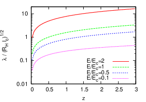
with and the Hubble radius. The resulting value of is plotted in fig. 2 as a function of and for different values of , adopting for definiteness. Note that Mpc.
One can now combine eqs. (7) and (11) with eq. (3) to obtain, after summation over all sources, that the flux from nuclei of charge is
| (12) |
One can hence define the final suppression factor of the fluxes as
| (13) |
i.e. as the ratio of the actual flux to the one that would be obtained for a continuous source distribution (corresponding to in eq. (12)). For this computation we can take , since we will be interested in scenarios for which the suppression happens for energies well below , and the results obtained are hence independent of . Note that once written in terms of , the suppression factor is the same for all nuclei.
The suppression factor is shown in fig. 3 adopting , and . The resulting values depend on the average distance between sources and the coherence length through the combination
| (14) |
and results are displayed for , 1, 2 and 5 as a function of . Approximate fits to these results can be obtained through the expression
| (15) |
with , , and . These fits are also shown in figure 3 with solid lines. Note that for the diffusion coefficient has the moderate energy dependence for the assumed Kolmogorov turbulence and hence the suppression factor decreases more slowly with decreasing energies, while for there is a strong energy dependence of the suppression factor and for different values of it is essentially just shifted in energy proportionally to .

The flux suppression is mainly due to the fact that at low energies CRs are unable to reach the Earth from the faraway sources and moreover they take a very long time to arrive to the Earth from the nearby ones, so that the low redshift contribution from these last is absent (in the diffusive regime the redshift gives a measure of propagation time rather than distance). Hence, the suppression factor has some sensitivity to source evolution effects because these determine the relative contribution to the flux arising from different redshifts. In fig. 4 we show the factor for and different assumptions on the cosmological parameters: the cases of source emissivity evolution as with (while in the remaining cases), the case and that for the magnetic field evolution parameter , besides the case corresponding to the parameters adopted in the previous figure. The results vary slightly, except if a very strong source emissivity evolution is adopted, what could lead to a reduced suppression (larger ) due to the larger contribution to the observed CRs from high-redshift (i.e. longer propagation times, allowing for more diffusion). In this case the suppression factor is similar in shape but gets shifted to lower values of . Hence, adopting a value for one finds that a given suppression factor would lead to inferred values of larger by a factor about 1.5 in the case of strong evolution with respect to what would be obtained in the case of uniform source evolution. We note that the evolution of the source emissivity considered here is not equivalent to assuming an evolution in the source density, since increasing this last would decrease the typical source distance, shifting the magnetic suppression effect also to lower energies but due to different physical reasons.

A necessary condition to have diffusion from the nearest source is that , and hence (with in eq. (2), from which one gets ). Moreover, for the flux from the nearest source to arrive in a typical time scale of the order of the Hubble time, so that the suppression is significant, one needs that and hence one needs, in the regime in which , that . Actually, looking at the detailed results in figure 3 we see that in the non-resonant diffusion regime (i.e. for ) the suppression factor starts to become noticeable () for and it reaches the value for the energy given by
| (16) |
Hence, introducing the corresponding rigidity value we find the following relation between the different parameters involved (valid for )
| (17) |
We note that the expression in eq. (12) is valid as long as the interaction energy losses are small. In the case of nuclei, if photo-disintegration processes produce some amount of secondaries these particles will diffuse similarly as their parent nuclei and their final suppression will then be similar44 4 Actually the suppression factor may be slightly larger for secondary nuclei due to their preferential production at relatively higher redshifts where Lorentz factors are larger and radiation backgrounds more relevant, but we ignore these effects which are not expected to lead to large differences.. We will hence apply in the following the suppression factor to the fluxes of both primary and secondary nuclei surviving at low energies.
We have checked that considering proton scenarios with large maximum energies ( eV) we obtain results consistent with the numerical simulations in [11] and [13] (after accounting for the slightly different diffusion coefficients adopted), while considering mixed composition scenarios with large maximum rigidities we obtain results consistent with those in [15, 6].
3 A scenario with transition to heavier elements
We will be interested in the following in scenarios with relatively low maximum rigidities, – EeV, like those considered in refs. [25, 26]. This is motivated by the observed trend in the mass composition measured by the Auger Observatory, which suggests a transition towards heavier elements starting above a few EeV, which would naturally result if the lighter elements can no longer be accelerated above the indicated cutoff energies. These ‘low cutoff scenarios’ have not been studied in detail in the presence of extra-galactic magnetic field effects (some qualitative considerations were given in [26]). Our analytic approximate treatment of diffusion effects together with the detailed results of CR propagation in the absence of magnetic fields obtained using the CRpropa code [27] allows us to obtain the predictions for the CR spectra and composition in these models.


As an illustration we show in fig. 5 the spectra and composition (both the average value of and its variance, ) for scenarios with source spectra with maximum rigidity EV. We assume that the source spectra consist of different fractions of the representative elements p, He, N, Si and Fe, which are indicated in the figure labels in each case. These fractions are chosen so as to approximately reproduce the observed spectra measured by the Auger Collaboration [28], which is also shown in the figure together with the one measured by the HiRes Collaboration [29]. The three panels correspond to no magnetic field effect (top), diffusion such that EV with (middle) and (bottom).
The extra-galactic fluxes are obtained using CRpropa and we incorporate the effects of magnetic field diffusion by multiplying the fluxes obtained for each final mass by the corresponding suppression factor , adopting the expression obtained in eq. (15). The spectra of the different mass groups as well as the total extra-galactic flux are displayed. In addition to the extra-galactic fluxes we also include an additional ‘galactic’ component so as to match the total spectrum down to EeV. This extra component may be just the high energy tail of the galactic CRs but may eventually also receive contributions from fainter but closer extra-galactic sources, less suppressed by magnetic diffusion effects.


The right panels in the figures show the expected average value of as well as its variance, and they are compared with the results inferred for these quantities from the measurements of the maximum of the longitudinal development of the showers and its fluctuations, determined with the fluorescence technique by the Auger Collaboration [30]. The results displayed correspond to the values inferred adopting the EPOS1.99 hadronic interaction model, with the shaded bands indicating the associated systematic uncertainties. Somewhat shifted results are obtained assuming different hadronic models to interpret the measurements (see [30]). We note that below 3 EeV the contribution from the ‘galactic’ component can be sizeable and it is relevant for the determination of the resulting composition. The values of and below 3 EeV hence depend on the assumed composition of this extra component. In fig. 5 we just assumed it consisted of nuclei with negligible variance (since this simple assumption led to a rough agreement with the observed values in the cases including magnetic diffusion). We show in fig. 6 how these predictions change for different assumptions on the value of for the extra component, for the cases of pure Fe, N and p. Had we assumed a non-negligible intrinsic variance in the mass composition of this extra component, the results for would have been slightly higher at EeV. In fig. 6 we adopted EV and EV, considering to illustrate how a steeper source spectra can also lead to reasonable results.


To illustrate the effect of the maximum rigidity cutoff adopted we show in fig. 7 the results for EV, with (top panel), and for EV, with (lower panel). The first one shows the tendency to increase the variance of when the light elements contribute up to higher energies, while the second one shows the tendency to increase when the cutoff is lowered. Finally, fig. 8 exemplifies the effect of the source luminosity evolution. It displays the results for the case of strong evolution of the source emissivity, i.e. with following the Gamma Ray Burst rate (corresponding to the SFR6 evolution obtained in [31]), adopting and EV. In this case the extragalactic proton component can be more enhanced below the ankle.


We should mention that the finite distance to the closest sources can also make the ‘GZK’ suppression at the highest energies stronger than in the case of a continuous source distribution (see [13, 15, 16]). However, this effect is expected to be more pronounced in scenarios with high rigidity cutoffs for which the effects of the ‘GZK’ suppression are important, while in the scenarios we considered with low rigidity cutoffs this should have only a minor impact, and the high energy suppression of the spectrum is largely due to the source acceleration cutoff itself rather than to the propagation effects. Given the arbitrariness in the shape of the cutoff function adopted, which ultimately models the suppression at the highest energies in our case, we do not include the additional suppression from the finite source distance effect at the highest energies.
In the previous plots of the spectrum and composition (figs. 5 to 8) we fixed the parameters and , which determine the shape and location respectively of the suppression due to the magnetic diffusion. These parameters are ultimately related to the extra-galactic turbulent magnetic field strength and coherence length as well as to the typical separation between sources (and hence to ), through eqs.(14) and (17). However, the relation between these quantities is not unique, so that different combinations of , and values can give rise to the same results. For instance, to have EV and would require that and (which can be obtained for instance with Mpc, Mpc and nG). On the other hand, if we consider a given value for one finds that for the shape of the suppression is essentially independent of so that the resulting spectra and composition will be quite independent of the actual value of , with this parameter just determining the value for inferred.
In the previous plots we did not attempt to obtain detailed fits to the Auger results but just tried to show that the diffusion in extra-galactic magnetic fields can help to give rise to the observed trends in and in scenarios compatible with Fermi acceleration (while fits to Auger results ignoring magnetic effects tend to prefer [25, 32, 6, 16]). Notice also that a detailed interpretation of the composition results depends actually on the assumed hadronic models. In addition, one should keep in mind that results from HiRes and Telescope Array are compatible with a light component even at energies above 10 EeV [20, 21]. Moreover, the spectrum is still affected by the systematics of the energy determination, as is evident from the differences between Auger and HiRes spectra.
4 Conclusions
In this work we have considered in detail the low energy spectral suppression appearing when the density of extra-galactic UHECR sources is low and CRs diffuse in turbulent extra-galactic magnetic fields. We obtained simple fits to the flux suppression factor valid in the limit in which adiabatic losses dominate over interaction ones, which holds for EeV. Scenarios in which the flux suppression appear in this energy regime are particularly relevant given the indications in favor of the presence of a significant light extra-galactic component at EeV energies. On the other hand, we considered scenarios with low maximum rigidities, –10) EV, in which a transition to heavier elements for increasing energies naturally occurs. The magnetic diffusion effects then allow to suppress the extragalactic nuclei contribution at EeV without requiring the introduction of very hard source spectra and can hence lead to results more consistent with the overall composition trends measured by the Auger Collaboration also for source spectra compatible with Fermi shock acceleration (–2.4).
Acknowledgments
We are grateful to D. Harari for useful discussions. We thank the authors of CRpropa for making their code public. Work supported by CONICET and ANPCyT, Argentina.
Appendix
In this Appendix we discuss the low energy attenuation of the proton spectrum in the case in which the energy losses due to pair creation off CMB photons are also included. This allows to illustrate their impact and shows the applicability of the results obtained with adiabatic losses alone.
We include pair creation losses off CMB photons following [33], from which we compute the energy loss coefficient due to interactions alone. Taking into account the redshift evolution of the CMB photon energy and of its density, one has that
| (18) |
with the value computed at . The original energy at redshift , , is then obtained by integrating the equation
| (19) |
which accounts for both adiabatic and pair production losses. Another relation which is necessary to compute in eq. (3) is (see Appendix in [34])
| (20) |
where to a good approximation one can use that d [34].


Combining all this we can then compute the suppression factor including energy losses due to pair production, with the results shown in fig. 9. We here adopted nG, Mpc (leading to EeV) and EeV (the results have only a mild dependence on the value of adopted). The left panel is the equivalent to fig. 3 while the right panel to fig. 4. As can be seen from the left panel the resulting suppression factors are essentially unchanged at low energies (solid lines represent the fits obtained ignoring pair creation losses which were also shown in fig. 3). Only in the cases in which EeV, corresponding to large values of (actually for EeV) the flux suppression has some noticeable changes, as in the case shown for , and to a minor extent for the case . For large the suppression is approximately similar in shape to that obtained ignoring pair losses but it is slightly shifted to higher energies. This also implies that the final spectra obtained assuming a given value of will be quite independent of whether pair production losses are included or not, but eventually what can change for large values of is the relation between and the underlying magnetic field parameters and source distances (tending to reduce the required values of ).
We note that when pair losses are included one finds that for EeV and at high redshifts the initial energy can be much larger than , showing an explosive increase with redshift as soon as EeV. When this happens, the contribution to arising from higher redshifts gets very suppressed. This explains the behavior observed, where the increased flux suppression is the result of the competition between two opposite effects. On one side the larger values of obtained including pair losses lead to larger values for , what would suggest that the flux should be less suppressed (see eq. (8)). However, the fact that higher redshifts contribute less to implies that the overall suppression, caused by the fact that CRs from nearby sources have not enough time to diffuse from small redshifts, ends up being stronger. The behavior of also explains why including pair losses the suppression factors become quite insensitive to the maximum redshift considered, as is apparent from the right panel in fig. 9.
We hence conclude that when pair creation losses are included the suppression factors for given values of and remain essentially unchanged as long as EeV. The case of nuclei should be similar (with the suppression factors below EeV remaining unaffected) but the inclusion of photo-disintegration effects would make the analysis more involved in this case.
References
- [1] D. Harari, S. Mollerach and E. Roulet, JHEP 0203 (2002) 045
- [2] G. Sigl, F. Miniati, T. Ensslin, Phys. Rev. D 70 (2004) 043007
- [3] K. Dolag et al., JETP Lett. 79, 583 (2004) [Pisma Zh.Eksp.Teor.Fiz.79:719 (2004)]
- [4] K. Kotera and M. Lemoine, Phys. Rev. D77 (2008) 023005
- [5] L.M. Widrow, Rev. Mod. Phys. 74 (2003) 775
- [6] D. Allard, Astropart. Phys. 39-40 (2012) 33
- [7] A. Achterberg et al., astro-ph/9907060
- [8] P. Blasi and A. Olinto, Phys. Rev. D59 (1999) 023001
- [9] T. Stanev et al., Phys. Rev. D62 (2000) 093005
- [10] H. Yoshiguchi et al., Astrophys. J 586 (2003) 1211
- [11] M. Lemoine, Phys. Rev. D71 (2005) 083007
- [12] V. Berezinsky and A.Z. Gazizov, Astrophys. J 643 (2006) 8
- [13] V. Berezinsky and A.Z. Gazizov, Astrophys. J 669 (2007) 684
- [14] G. Sigl, Phys. Rev. D75 (2007) 103001
- [15] N. Globus, D. Allard and E. Parizot, Astron. & Astrophys. 479 (2008) 97
- [16] A.M. Taylor, M. Ahlers and F.A. Aharonian, Phys. Rev. D84 (2011) 105007
- [17] S.I. Syrovatskii, Soviet Astron. 3 (1959) 22
- [18] R. Aloisio and V. Berezinsky, Astrophys. J 612 (2004) 900
- [19] J. Abraham et al. (the Pierre Auger Collaboration), Phys. Rev. Lett. 104 (2010) 091101
- [20] R.U. Abbasi et al. (the High Resolution Fly’s Eye Collaboration), Phys. Rev. Lett. 104 (2010) 161101
- [21] Y. Tameda et al. (the Telescope Array Collaboration), Proc. of the 32nd ICRC, Beijing (2011)
- [22] P. Abreu et al. (the Pierre Auger Collaboration), Astrophys. J Lett. 762 (2012) L13
- [23] F. Casse, M. Lemoine and G. Pelletier, Phys. Rev. D 65 (2002) 023002
- [24] J. Candia and E. Roulet, JCAP 0410 (2004) 007
- [25] D. Allard, arXiv:0906.3156 [astro-ph.HE] (2009)
- [26] R. Aloisio, V. Berezinsky and A. Gazizov, Astropart. Phys. 34 (2011) 620
- [27] K.-H. Kampert et al., Astropart. Phys. 42 (2013) 41
- [28] J. Abraham et al. (the Pierre Auger Collaboration), Physics Letters B 685 (2010) 239; F. Salamida (for the Pierre Auger Collaboration), 32nd ICRC, Beijing 2011, arXiv:1107.4809 [astro-ph.HE]
- [29] R. Abbasi et al. (the HiRes Collaboration), Phys. Rev. Lett. 100 (2008) 101101
- [30] P. Abreu et al. (the Pierre Auger Collaboration), JCAP 1302 (2013) 026
- [31] T. Le and Ch. Dermer, Astrophys. J. 661 (2007) 394
- [32] D. Hooper and A.M. Taylor, Astropart. Phys. 33 (2010) 151
- [33] M.J. Chodorowski, A.A. Zdziarski and M. Sikora, Astrophys. J. 400 (1992) 181
- [34] V. Berezinsky, A.Z. Gazizov, S.I. Grigorieva, Phys.Rev. D47 (2006) 043005