跳到论文正文
W Papers独立论文阅读器 arXiv:1305.6491 论文正文 计算阅读时间 · 0%
引用这篇论文根据当前论文元数据生成,正式投稿前建议核对。


License: arXiv.org perpetual non-exclusive license
arXiv:1305.6491v1 [math.PR] 28 May 2013

Lévy processes with marked jumps II :
Application to a population model with mutations at birth

Cécile Delaporte Note: UPMC Univ. Paris 6, Laboratoire de probabilités et modèles aléatoires CNRS UMR 7599, and Collège de France, Center for interdisciplinary research in biology CNRS UMR 7241 ; e-mail : cecile.delaporte@upmc.fr
Remerciements

I would like to thank my supervisor, Amaury Lambert, for his very helpful advice and encouragement.

Key words and phrases : splitting tree, coalescent point process, Poisson point process, invariance principle, Lévy process, excursion theory.
AMS Classification : 60J85,60F17 (Primary), 92D25, 60G55, 60G51, 60J55 (Secondary)

1 Introduction

A splitting tree ([11], [12], [17]) describes a population of individuals with i.i.d. lifetime durations, which distribution is not necessarily exponential, giving birth at constant rate during their lives. Each birth gives rise to a single child, who behaves as an independent copy of her parent. We consider here the extended framework of [17] : for each individual, the birth times and lifetimes of her progeny is given by a Poisson process with intensity d​t⋅Λ⁡(d​r)\text{d}t\cdot\Lambda(\text{d}r), where the so-called lifespan measure Λ\Lambda is a Lévy measure on (0,∞)(0,\infty) satisfying ∫(1∧r)​Λ​(d​r)<∞\int(1\wedge r)\Lambda(\text{d}r)<\infty. In particular, the number of children of a given individual is possibly infinite. In addition, we assume that individuals carry types, and that every time a birth occurs, a mutation may happen, giving rise to a mutant child. Mutations are assumed to be neutral, meaning that they do not affect the behaviour of individuals. In order to take this into account, we introduce marked splitting trees : to each birth event we associate a mark in {0,1}\{0,1\}, which will code for the absence (00) or presence (11) of a mutation. In other words, a 00-type birth means a clonal birth, and a 11-type birth produces a mutant child. The mutations experienced by the population are then described by these marks.

Population models with mutations have inspired lots of works in the past, and have many applications in domains such as population genetics, phylogeny or epidemiology. Such models have been well studied in the particular case of populations with fixed size. In the Wright-Fisher and Moran models with neutral mutations, as well as in the Kingman coalescent, explicit results on the allelic partition of the population are provided by Ewens’ sampling formula ([10],[9]). Relaxing the hypotheses of constant population size, branching processes with mutations at birth are studied in the monography [25]. More recently, results have been obtained for the allelic partition and frequency spectrum of splitting trees, with mutations appearing either at birth of individuals ([24]) or at constant rate along the lineages ([18], [5], [6]), and are reviewed in [7]. The present work focuses on asymptotic results when the size of the population gets large, for the genealogy (with mutational history) of splitting trees with mutations at birth, and relies on a previous article [8].

Genealogy of the nn-th population

Let us fix some positive real number τ\tau. For n∈ℕn\in\mathbb{N}, consider a marked splitting tree 𝕋n\mathbb{T}_{n}, and condition it on having a fixed positive number InI_{n} of individuals alive at level τ\tau. Note that we use here the word ’level’ to denote the real time in which the individuals live, whereas we reserve the word ’time’ for the index of stochastic processes. This paper follows on from a work of L. Popovic ([23]) in the critical case with exponential lifetimes, without mutations, in which she proved the convergence in distribution of the coalescent point process (i.e. the smallest subtree containing the genealogy of the extant individuals) towards a certain Poisson point process. Our aim is to provide asymptotic results as InI_{n} gets large, for the structure of the genealogy of the population up to level τ\tau, enriched with the random levels at which marks occurred on the lineages. To this aim, after a proper rescaling of 𝕋n\mathbb{T}_{n}, we introduce a random point measure Σn\Sigma_{n} which we call the marked coalescent point process. This point measure has In−1I_{n}-1 atoms  ; its ii-th one is itself a random point measure, whose set of atoms contains all the levels where mutations occurred on the ii-th lineage, and the coalescence time between individuals ii and i−1i-1. This sequence of point measures (Σn)(\Sigma_{n}) is the mathematical object for which we aim to get convergence as n→∞n\to\infty, after having set some convergence assumptions, which we discuss later.

Our work mainly relies on the study of splitting trees with the help of the so-called jumping chronological contour process (or JCCP). This process is an exploration process of the tree (without mutations) introduced by A. Lambert in [17], visiting all the existence levels of all the individuals exactly once, and ending at level 00. He showed in this paper that the JCCP of a tree truncated up to level τ\tau is a compensated compound Poisson process with no negative jumps (spectrally positive Lévy process with finite variation) reflected below τ\tau and killed when hitting 00. In particular, the labeling of the excursions of the JCCP below τ\tau provides a labeling of the extant individuals at level τ\tau. Inferring properties concerning the genealogy of the alive population at level τ\tau in the tree then essentially consists in studying the excursions away from τ\tau of this reflected Lévy process.

We introduce in [8] a generalization of this contour process to the framework of our rescaled marked splitting trees (𝕋~n)(\tilde{\mathbb{T}}_{n}). We are thereby led to study a bivariate Lévy process (Z~n,Z~nm)(\tilde{Z}_{n},\tilde{Z}_{n}^{\textsc{m}}). Roughly speaking, Z~n\tilde{Z}_{n} codes for the JCCP of 𝕋~n\tilde{\mathbb{T}}_{n} (without mutations), and Z~nm\tilde{Z}_{n}^{\textsc{m}} codes for the mutations. Namely, since a jump of Z~n\tilde{Z}_{n} corresponds to the encounter of a birth event when exploring the tree, Z~nm\tilde{Z}_{n}^{\textsc{m}} will jump as well (with amplitude 1) if this birth was of type 11. The process (Z~n,Z~nm)(\tilde{Z}_{n},\tilde{Z}_{n}^{\textsc{m}}) is in one-to-one correspondence with the marked tree 𝕋~n\tilde{\mathbb{T}}_{n}. We now want to characterize the law of the atoms of Σn\Sigma_{n} using this property. Let us first give an idea of our reasoning in the case where there is no mutations. The JCCP of 𝕋~n\tilde{\mathbb{T}}_{n}, truncated up to τ\tau, is distributed as Z~n\tilde{Z}_{n} reflected below τ\tau. The set of levels at which births occurred on the lineage of the ii-th individual, up to its coalescence with the rest of the tree, is then exactly the set of values taken by the future infimum of the ii-th excursion of the JCCP under τ\tau. First, this entails that the atoms of Σn\Sigma_{n} are i.i.d. Second, using a time reversal argument, the distribution of this set can be read from the ascending ladder height process of Z~n\tilde{Z}_{n}. A similar reasoning for the splitting tree with mutations leads to the following facts. Consider Hn+H^{+}_{n} the ascending ladder height process of Z~n\tilde{Z}_{n}, and put marks on its jumps in agreement with the marks on the corresponding jumps of Z~n\tilde{Z}_{n}. Note that this implies a selection of the marks that are carried by jumps of the supremum process of Z~n\tilde{Z}_{n}. Denoting by HnmH^{\textsc{m}}_{n} the counting process of these marks, the bivariate process (Hn+,Hnm)(H^{+}_{n},H^{\textsc{m}}_{n}) is a (possibly killed) bivariate subordinator which we call the marked ladder height process. The mutations on a lineage form then an inhomogeneous regenerative set, distributed as the image by Hn+H^{+}_{n} of the jump times of HnmH^{\textsc{m}}_{n} under the excursion measure of Z~n\tilde{Z}_{n} away from 00, which finally yields a simple description of the law of the (i.i.d.) atoms of Σn\Sigma_{n}.

Convergence results

Obtaining an invariance principle for a population model in a large population asymptotic requires to assume that as n→∞n\to\infty, the population converges in a certain sense. A classical example would be the convergence of the rescaled Bienaymé-Galton-Watson process towards the Feller diffusion ([20]). Now regardless of mutations, the JCCP offers a one-to-one correspondence between 𝕋n\mathbb{T}_{n} and a continuous time process. Our first assumption arises then naturally as the convergence in distribution of the properly rescaled Lévy process Z~n\tilde{Z}_{n} towards a Lévy process ZZ (with infinite variation, Assumption A). In particular, the lifetimes of individuals do not necessarily vanish in the limit. Besides, two different assumptions concerning the mutations are considered. The first one (B.1) falls within the classical asymptotic of rare mutations : every birth is of type 11 with a constant probability θn\theta_{n}, and θn→0\theta_{n}\to 0 as n→∞n\to\infty. Asymptotic results in this framework are obtained in [4] for the genealogical structure of alleles in a critical or subcritical Bienaymé-Galton-Watson process (however contrary to ours, they do not concern the extant population at a fixed time horizon, but the whole population). The second one (B.2) examines the case where the probability of an individual to be a mutant is correlated with her lifetime, in the sense that mutations favor longer lifetimes.

While Assumption A alone ensures the convergence in distribution of Hn+H^{+}_{n} towards the classical ladder height process of ZZ, Assumptions B.1 and B.2 are designed to allow that of the marked ladder height process. Indeed, we prove in [8] the convergence in law of (Hn+,Hnm)(H^{+}_{n},H^{\textsc{m}}_{n}) towards a (possibly killed) bivariate subordinator (H+,Hm)(H^{+},H^{\textsc{m}}), such that H+H^{+} is the ladder height process of ZZ. Note nevertheless that in this framework there is in general no convergence of the whole mutation process, namely Z~nm\tilde{Z}_{n}^{\textsc{m}}. In the case of Assumption B.1, H+H^{+} and HmH^{\textsc{m}} are independent, and HmH^{\textsc{m}} is a Poisson process with parameter θ\theta, which arises as the limit of the sequence θn\theta_{n} after a proper rescaling. This means that the contribution to the mutations in the limit exclusively comes from individuals with vanishing lifetimes. This is no longer the case under Assumption B.2, yet additional independent marks can appear if ZZ has a Gaussian component. Using this convergence to deduce that of the (rescaled) law of the mutations on a lineage, the convergence of (Σn)(\Sigma_{n}) to a Poisson point measure is then a straightforward consequence of the law of rare events for null arrays (see e.g. [14, Th. 16.18]). Under B.1, its intensity measure is the law of the image by H+H^{+} of an independent Poisson process with parameter θ\theta, under the excursion measure of ZZ away from zero. A very similar but slightly more complicated result, involving the limiting marked ladder height process (H+,Hm)(H^{+},H^{\textsc{m}}), is available under B.2. Besides, in the case where ZZ is a Brownian motion, H+H^{+} is simply a drift, and thus the intensity measure is the law of a Poisson process killed at some independent random time, distributed as the depth of an excursion of the Brownian motion away from 0.

Outline

The paper is organized as follows : Section 2 sets up notation for the topological framework, and provides some background on the excursion theory for Lévy processes (see e.g. [3] and [16]). Section 3 is devoted to the statement of our results, and Section 4 to their proofs. In the appendix, we give proof of some properties that are consequences of Assumption A, and which we make frequent use of throughout the paper.

2 Preliminaries

2.1 Topology

We consider the Euclidean space ℝd\mathbb{R}^{d} and endow it with its Borel σ\sigma-field ℬ⁡(ℝd)\mathcal{B}(\mathbb{R}^{d}). We denote by 𝔻⁡(ℝd)\mathbb{D}(\mathbb{R}^{d}) the space of all càd-làg functions from ℝ+\mathbb{R}_{+} to ℝd\mathbb{R}^{d}. We endow the latter with the Skorokhod topology, which makes it a Polish space (see [13, VI.1.b]). In the sequel, for any function f∈𝔻⁡(ℝ)f\in\mathbb{D}(\mathbb{R}) and x>0x>0, we will use the notation Δ​f​(x)=f⁡(x)−f⁡(x−)\Delta f(x)=f(x)-f(x-), where f⁡(x−)=limu→x,u<xf⁡(u)f(x-)=\lim_{u\to x,\,u<x}f(u).

Now for any Polish space XX, with its Borel σ\sigma-field ℬ\mathcal{B}, the space ℳf​(X)\mathcal{M}_{f}(X) of positive finite measures on (X,ℬ)(X,\mathcal{B}) can be endowed with the weak topology : It is the coarsest topology for which the mappings μ↦∫f​d​μ\mu\mapsto\int f\text{d}\mu are continuous for any continuous bounded function ff. In the sequel, we will use the notation μ⁡(f):=∫f​d​μ\mu(f):=\int f\text{d}\mu.

Hence we endow here ℳf​(ℝd)\mathcal{M}_{f}(\mathbb{R}^{d}) and ℳf​(𝔻​(ℝd))\mathcal{M}_{f}(\mathbb{D}(\mathbb{R}^{d})) with their respective weak topologies. The notation ⇒\Rightarrow will be used for both weak convergence in ℝd\mathbb{R}^{d} and in 𝔻⁡(ℝd)\mathbb{D}(\mathbb{R}^{d}), and we will use the symbol =(d)\stackrel{{\scriptstyle(d)}}{{=}} for the equality in distribution. Recall that for any sequence of ℝd\mathbb{R}^{d}-valued càd-làg processes (Xn)(X_{n}), the weak convergence of (Xn)(X_{n}) towards a process XX of 𝔻⁡(ℝd)\mathbb{D}(\mathbb{R}^{d}) is equivalent to the finite dimensional convergence of (Xn)(X_{n}) towards XX along any dense subset D⊂ℝ+D\subset\mathbb{R}_{+}, together with the tightness of (Xn)(X_{n}). For more details about convergence in distribution in 𝔻⁡(ℝd)\mathbb{D}(\mathbb{R}^{d}), see [13, VI.3].

From now on, we fix τ>0\tau>0. We consider the space of positive point measures on (0,τ)×{0,1}(0,\tau)\times\{0,1\}, and endow it with the σ\sigma-field generated by the mappings {pB:ξ↦ξ(B),B∈ℬ((0,τ))⊗𝒫({0,1})}\{p_{B}:\xi\mapsto\xi(B),\ B\in\mathcal{B}((0,\tau))\otimes\mathscr{P}(\{0,1\})\}. Then we denote by ℳP\mathcal{M}_{\textsc{P}} the subset of the point measures on (0,τ)×{0,1}(0,\tau)\times\{0,1\} of the form

δ(am​,0)+∑i=0m−1δ(ai​,1), where ​m∈ℤ+​ and ​0<a0<…<am−1≤am<τ.\delta_{(a_{m},0)}+\sum_{i=0}^{m-1}\delta_{(a_{i},1)},\text{ where }m\in\mathbb{Z}_{+}\text{ and }0<a_{0}<\ldots<a_{m-1}\leq a_{m}<\tau.

The trace σ\sigma-field on ℳP\mathcal{M}_{\textsc{P}} is in particular generated by the class

𝒞={pB,B=[ε,τ)×{0},B=[ε,τ)×{1}}ε∈(0,τ).\mathscr{C}=\big\{p_{B},\ B=[\varepsilon,\tau)\times\{0\},\ B=[\varepsilon,\tau)\times\{1\}\big\}_{\varepsilon\in(0,\tau)}.

2.2 Excursion theory for spectrally positive Lévy processes

We provide here some background about the excursion theory for spectrally positive Lévy processes. For the basic properties concerning spectrally positive Lévy processes that will be needed here, we refer to a summary we provide in [8, Section 2] (these properties can otherwise be found in [3] or [16], for example).

Let XX be a spectrally positive Lévy process with Lévy measure Λ\Lambda. We define its past supremum X¯t:=sup[0,t]​X\bar{X}_{t}:=\underset{[0,t]}{\sup}X for all t≥0t\geq 0. We denote by ℰ\mathscr{E} the set of excursions of X−X¯X-\bar{X} away from 00 : ℰ\mathscr{E} is the set of the càd-làg functions ϵ\epsilon with no negative jumps for which there exists ζ=ζ⁡(ϵ)∈(0,∞]\zeta=\zeta(\epsilon)\in(0,\infty], which will be called the lifetime of the excursion, and such that ϵ⁡(0)=0\epsilon(0)=0, ϵ⁡(t)\epsilon(t) has values in (−∞​,0)(-\infty,0) for t∈(0,ζ)t\in(0,\zeta) and in the case where ζ<∞\zeta<\infty, ϵ⁡(ζ)∈[0,∞)\epsilon(\zeta)\in[0,\infty).

The reflected process X−X¯X-\bar{X} is a Markov process for which one can construct (Lt)t≥0(L_{t})_{t\geq 0} a local time at 0. We denote by L−1L^{-1} its inverse, and we consider the process e=(et)t≥0e=(e_{t})_{t\geq 0} with values in ℰ∪{∂}\mathscr{E}\cup\{\partial\} (where ∂\partial is an additional isolated point), defined by :

et:={((X−X¯)s+L−1​(t−)​,0≤s<L−1​(t)−L−1​(t−))if ​L−1​(t−)<L−1​(t)∂elsee_{t}:=\left\{\begin{array}[]{l l}((X-\bar{X})_{s+L^{-1}(t-)},0\leq s<L^{-1}(t)-L^{-1}(t-))&\quad\text{if }L^{-1}(t-)<L^{-1}(t)\\ \partial&\quad\text{else}\\ \end{array}\right.

Then according to Theorem IV.10 in [3], if XX does not drift to −∞-\infty, then 00 is recurrent for the reflected process, and (t,et)t≥0(t,e_{t})_{t\geq 0} is a Poisson point process with intensity c​d​t​N​(d​ϵ)c\;\text{d}t\ N(\text{d}\epsilon), where cc is some constant depending on the choice of LL, and NN is a measure on ℰ\mathscr{E}. Else, (t,et)t≥0(t,e_{t})_{t\geq 0} is a Poisson point process with intensity c​d​t​N​(d​ϵ)c\;\text{d}t\ N(\text{d}\epsilon), stopped at the first excursion with infinite lifetime.

In the same way, we denote by ℰ′\mathscr{E}^{\prime} the set of excursions of XX away from 00 : ℰ′\mathscr{E}^{\prime} is the set of the càd-làg functions ϵ\epsilon with no negative jumps for which there exists ζ=ζ⁡(ϵ)∈(0,∞]\zeta=\zeta(\epsilon)\in(0,\infty], and such that ϵ⁡(0)=0\epsilon(0)=0, ϵ⁡(t)\epsilon(t) has values in ℝ∗\mathbb{R}^{*} for t∈(0,ζ)t\in(0,\zeta), and ϵ⁡(ζ)=0\epsilon(\zeta)=0 if ζ<∞\zeta<\infty. We then introduce χ⁡(ϵ):=inf{t∈(0,ζ],ϵ⁡(t)∈[0,∞)}\chi(\epsilon):=\inf\{t\in(0,\zeta],\ \epsilon(t)\in[0,\infty)\}.

Denoting by ℒ\mathscr{L} a local time at 00 of XX and by ℒ−1\mathscr{L}^{-1} its inverse, we define the process e′=(et′)t≥0e^{\prime}=(e^{\prime}_{t})_{t\geq 0} with values in ℰ′∪{∂}\mathscr{E}^{\prime}\cup\{\partial\}

et′:={(Xs+ℒ−1​(t−)​,0≤s<ℒ−1​(t)−ℒ−1​(t−))if ​ℒ−1​(t−)<ℒ−1​(t)∂elsee^{\prime}_{t}:=\left\{\begin{array}[]{l l}(X_{s+\mathscr{L}^{-1}(t-)},0\leq s<\mathscr{L}^{-1}(t)-\mathscr{L}^{-1}(t-))&\quad\text{if }\mathscr{L}^{-1}(t-)<\mathscr{L}^{-1}(t)\\ \partial&\quad\text{else}\\ \end{array}\right.

If XX has no Gaussian component, any excursion et′∈ℰ′e^{\prime}_{t}\in\mathscr{E}^{\prime} first visits (−∞​,0)(-\infty,0), and we necessarily have χ⁡(et′)>0\chi(e^{\prime}_{t})>0 (but possibly infinite). On the other hand, if XX has a Gaussian component, it can creep upwards and then χ⁡(et′)∈[0,∞]\chi(e^{\prime}_{t})\in[0,\infty]. Again, according to Theorem IV.10 in [3], e′e^{\prime} is a Poisson point process with intensity c′​d​t​N′​(d​ϵ)c^{\prime}\;\text{d}t\ N^{\prime}(\text{d}\epsilon), stopped if XX is subcritical at the first excursion with infinite lifetime. Here c′c^{\prime} is some constant depending on the choice of ℒ\mathscr{L} and N′N^{\prime} a measure on ℰ′\mathscr{E}^{\prime}.

Finally, we describe some marginals of NN and N′N^{\prime} in the proposition below, for which we refer to [16, Th. 6.15 and (8.29)], [1, (3)] and [2, Cor. 1].

Proposition 2.1.

We have for all z,x>0z,x>0 :

  1. (i)

    If XX has finite variation,

    N(−ϵ(ζ−)∈dx,ϵ(ζ)∈dz,ζ<∞)=W(0)e−η​xdxΛ(x+dz)N(-\epsilon(\zeta-)\in\text{d}x,\ \epsilon(\zeta)\in\text{d}z,\ \zeta<\infty)=W(0)e^{-\eta x}\text{d}x\Lambda(x+\text{d}z)
  2. (ii)

    If XX has infinite variation and no Gaussian component (i.e. b=0b=0),

    N(−ϵ(ζ−)∈dx,ϵ(ζ)∈dz,ζ<∞)=e−η​xdxΛ(x+dz).N(-\epsilon(\zeta-)\in\text{d}x,\ \epsilon(\zeta)\in\text{d}z,\ \zeta<\infty)=e^{-\eta x}\text{d}x\Lambda(x+\text{d}z).

Moreover, in both cases, under N(⋅|−ϵ(ζ−)=x,ζ<∞)N(\,\cdot\,\,|\,-\epsilon(\zeta-)=x,\ \zeta<\infty), the reversed excursion

(−ϵ⁡((ζ−t)−)​, 0≤t<ζ)\big(-\epsilon((\zeta-t)-),\ 0\leq t<\zeta\big)

is equal in law to (Xt​, 0≤t<T0)(X_{t},\ 0\leq t<T^{0}) under ℙx(⋅|T0<∞)\mathbb{P}_{x}(\,\cdot\,\,|\,T^{0}<\infty).

Finally, the same statement holds replacing NN by N′N^{\prime} and ζ\zeta by χ\chi.

3 A limit theorem for splitting trees with mutations at birth

3.1 JCCP of a marked splitting tree

Formally, a splitting tree (without mutations) is a random real tree characterized by a σ\sigma-finite measure Λ\Lambda on (0,∞)(0,\infty), satisfying ∫(1∧u)​Λ​(d​u)<∞\int(1\wedge u)\Lambda(\text{d}u)<\infty. Consider such a splitting tree, and assume first that there is extinction of the population. In [17], A. Lambert considers a contour process of this tree called JCCP (jumping chronological contour process). He establishes that the tree and its contour process are in one-to-one correspondence and characterizes the law of the latter : conditional on the first individual in the tree to have life duration xx, its JCCP is distributed as a finite variation, spectrally positive Lévy process with drift −1-1 and Lévy measure Λ\Lambda, starting at xx, and killed upon hitting 00. In the case of non extinction, we then can consider the JCCP of the tree truncated up to level τ\tau, which has the law of the Lévy process described above, starting at x∧τx\wedge\tau, and reflected below level τ\tau. As noticed in Section 1, the exploration of the tree by its JCCP defines a way of ordering the individuals. In the sequel, when we label the extant individuals at level τ\tau, we refer to that order.

Consider now a marked splitting tree 𝕋\mathbb{T} as defined in Section 1. We assume that the probability for a child to be a mutant can only (possibly) depend on her life span uu, and if we denote by f⁡(u)f(u) this probability, where ff is a function from ℝ+∗\mathbb{R}_{+}^{*} to [0,1][0,1], ff will be called the mutation function of the tree. Then 𝕋\mathbb{T} is characterized by its mutation function ff and its lifespan measure Λ\Lambda.

Then similarly as in the case without mutations, we define the JCCP of 𝕋\mathbb{T}. First assume that there is extinction of its population. Then the JCCP of the marked tree 𝕋\mathbb{T} is a bivariate process (Z,Zm)(Z,Z^{\textsc{m}}) from ℝ+\mathbb{R}_{+} to ℝ+×ℤ+\mathbb{R}_{+}\times\mathbb{Z}_{+}, whose first coordinate ZZ is the JCCP of the splitting tree without marks, and whose second coordinate ZmZ^{\textsc{m}} is the counting process of the mutations (see Figure 1). More precisely, for every jump time of ZZ (which corresponds to the encounter of a birth event in the exploration process), ZmZ^{\textsc{m}} jumps (with amplitude 11) iff this birth was a 11-type birth. Hereafter we say that a jump of ZZ occurring at time tt carries a mark (or a mutation) if Δ​Zm​(t)=1\Delta Z^{\textsc{m}}(t)=1.

This bivariate process is in one-to-one correspondence with 𝕋\mathbb{T}. Besides, conditional on the first individual to have life duration xx, it is distributed as a bivariate Lévy process with drift (−1,0)(-1,0), and Lévy measure Λ⁡(d​u)​𝔹f⁡(u)​(d​q)\Lambda(\text{d}u)\mathbb{B}_{f(u)}(\text{d}q) (where 𝔹r\mathbb{B}_{r} denotes the Bernoulli probability measure with parameter rr), starting at (x​,0)(x,0), and killed as soon as its first coordinate hits 00. As in the non-marked case, if the assumption of extinction does not hold, the law of the JCCP of the truncated tree can be obtained from the Lévy process we just described.

Refer to caption
Figure 1: a) A marked splitting tree : the vertical axis indicates chronological levels  ; the horizontal axis has no meaning, but the horizontal lines show filiation. The marks in the tree are symbolized by stars.
b) The associated JCCP (Z,Zm)(Z,Z^{\textsc{m}}) : ZZ is the classical JCCP of the (non-marked) tree represented in a)  ; the counting process of the mutations ZmZ^{\textsc{m}} is not drawn as a jump process on ℝ+\mathbb{R}_{+}, but is represented by the sequence of its jump times, which are symbolized by stars on the horizontal axis.

3.2 Definitions and notation

3.2.1 Rescaling the population

Let (Λn)n≥1(\Lambda_{n})_{n\geq 1} be a sequence of measures on (ℝ+∗,ℬ⁡(ℝ+∗))(\mathbb{R}_{+}^{*},\mathcal{B}(\mathbb{R}_{+}^{*})) satisfying ∫(1∧u)​Λn​(d​u)<∞\int(1\wedge u)\Lambda_{n}(\text{d}u)<\infty for all nn, and (fn)n≥1(f_{n})_{n\geq 1} a sequence of continuous functions from ℝ+\mathbb{R}^{+} to [0,1][0,1].

We now consider a sequence of marked splitting trees (𝕋n)n≥1(\mathbb{T}_{n})_{n\geq 1} such that for all nn, 𝕋n\mathbb{T}_{n} has lifespan measure Λn\Lambda_{n}, and mutation function fnf_{n}. Recalling that 𝔹r\mathbb{B}_{r} denotes the Bernoulli probability measure with parameter rr, we consider (Zn,Znm)(Z_{n},Z_{n}^{\textsc{m}}) an independent bivariate Lévy process with finite variation, Lévy measure Λn​(d​u)​𝔹fn​(u)​(d​q)\Lambda_{n}(\text{d}u)\mathbb{B}_{f_{n}(u)}(\text{d}q) and drift (−1,0)(-1,0), and make the following assumption :

Assumption A : There exists a sequence of positive real numbers (dn)n≥1(d_{n})_{n\geq 1} such that as n→∞n\to\infty, the process defined by

Z~n:=(1n​Zn​(dn​t))t≥0\tilde{Z}_{n}:=\Big(\frac{1}{n}Z_{n}(d_{n}t)\Big)_{t\geq 0}

converges in distribution to a (necessarily spectrally positive) Lévy process ZZ with infinite variation. We denote by Λ\Lambda its Lévy measure and by bb its Gaussian coefficient (b∈ℝ+b\in\mathbb{R}_{+}).

For all n∈ℕn\in\mathbb{N} and for all t≥0t\geq 0, set Z~nm​(t):=Znm​(dn​t)\tilde{Z}_{n}^{\textsc{m}}(t):=Z_{n}^{\textsc{m}}(d_{n}t). With an abuse of notation, the law of (Z~n,Z~nm)(\tilde{Z}_{n},\tilde{Z}_{n}^{\textsc{m}}) conditional on (Z~n​(0),Z~nm​(0))=(x​,0)(\tilde{Z}_{n}(0),\tilde{Z}_{n}^{\textsc{m}}(0))=(x,0), and the law of ZZ conditional on Z⁡(0)=xZ(0)=x, will both be denoted by ℙx\mathbb{P}_{x}, and we write ℙ\mathbb{P} for ℙ0\mathbb{P}_{0}.

Denote by 𝕋~n\tilde{\mathbb{T}}_{n} the splitting tree obtained from 𝕋n\mathbb{T}_{n} by rescaling the branch lengths by a factor 1n\frac{1}{n}. The introduction of the process (Z~n,Z~nm)(\tilde{Z}_{n},\tilde{Z}_{n}^{\textsc{m}}) is motivated by its fundamental role in the characterization of the law of the JCCP of 𝕋~n\tilde{\mathbb{T}}_{n} truncated up to level τ\tau (see later Lemma 4.8).

Some notation :

The Laplace exponents ψn\psi_{n} of ZnZ_{n}, ψ~n\tilde{\psi}_{n} of Z~n\tilde{Z}_{n} and ψ\psi of ZZ are defined by

𝔼⁡(e−λ​Zn​(t))=et​ψn​(λ),𝔼⁡(e−λ​Z~n​(t))=et​ψ~n​(λ)​ and ​𝔼​(e−λ​Z​(t))=et​ψ​(λ),λ≥0.\mathbb{E}(e^{-\lambda Z_{n}(t)})=e^{t\psi_{n}(\lambda)},\ \mathbb{E}(e^{-\lambda\tilde{Z}_{n}(t)})=e^{t\tilde{\psi}_{n}(\lambda)}\ \text{ and }\ \mathbb{E}(e^{-\lambda Z(t)})=e^{t\psi(\lambda)},\ \ \ \lambda\geq 0.

We denote by η~n\tilde{\eta}_{n} (resp. η\eta) the largest root of ψ~n\tilde{\psi}_{n} (resp. ψ\psi) and by ϕ~n\tilde{\phi}_{n} (resp. ϕ\phi) the inverse of ψ~n\tilde{\psi}_{n} (resp. ψ\psi) on [η~n,∞)[\tilde{\eta}_{n},\infty) (resp. [η,∞)[\eta,\infty)). We denote by W~n\tilde{W}_{n} (resp. WW) the scale function of Z~n\tilde{Z}_{n} (resp. ZZ). Finally, we denote by Λ~n\tilde{\Lambda}_{n} the Lévy measure of Z~n\tilde{Z}_{n}.

Remarks about (dn)(d_{n}) :

Writing for λ≥0\lambda\geq 0, 𝔼⁡(e−λ​Z~n​(t))=edn​t​ψn​(λ/n)\mathbb{E}(e^{-\lambda\tilde{Z}_{n}(t)})=e^{d_{n}t\psi_{n}(\lambda/n)}, we get from the Lévy-Khintchine formula [8, (2)] that Z~n\tilde{Z}_{n} has drift −dnn-\frac{d_{n}}{n}, Lévy measure Λ~n=dnΛn(n⋅)\tilde{\Lambda}_{n}=d_{n}\Lambda_{n}(n\cdot) and Laplace exponent ψ~n=dnψ(⋅/n)\tilde{\psi}_{n}=d_{n}\psi(\cdot/n). In particular, this gives W~n​(0)=n/dn\tilde{W}_{n}(0)=n/d_{n}. We prove in the appendix that W~n\tilde{W}_{n} converges pointwise to WW as n→∞n\to\infty, and besides, the assumption of infinite variation of ZZ ensures W⁡(0)=0W(0)=0. Thereby we know that necessarily dnn→∞\frac{d_{n}}{n}\to\infty as n→∞n\to\infty.

3.2.2 Asymptotic for the mutations

In order to allow the convergence in distribution of the mutation levels on the lineages, we have to make some technical assumptions on the mutation functions fnf_{n}. Here we suggest two possible assumptions : in the first one, the probability of a child in 𝕋n\mathbb{T}_{n} to be a mutant is constant, while in the second one, this probability depends on its life duration.

Assumption B.1 :

  1. (a)

    For all n≥1n\geq 1, for all u∈ℝ+u\in\mathbb{R}_{+}, fn​(u)=θnf_{n}(u)=\theta_{n}, where θn∈[0,1]\theta_{n}\in[0,1].

  2. (b)

    As n→∞n\to\infty, dnn​θn\frac{d_{n}}{n}\theta_{n} converges to some finite real number θ\theta.

Assumption B.2 :

  1. (a)

    The sequence (u↦fn​(n​u)1∧u)\big(u\mapsto\frac{f_{n}(nu)}{1\wedge u}\big) converges uniformly to u↦f⁡(u)1∧uu\mapsto\frac{f(u)}{1\wedge u} on ℝ+∗\mathbb{R}_{+}^{*}.

  2. (b)

    There exists κ≥0\kappa\geq 0 such that f⁡(u)/u→κf(u)/u\to\kappa as u→0+u\to 0^{+}.

Note that in B.1, necessarily θn→0\theta_{n}\to 0 as n→∞n\to\infty, corresponding to the classical rare mutation asymptotic. Then if we denote by ff the limit of the sequence (fn)(f_{n}), we have f≡0f\equiv 0. Besides, in Assumption B.2 the choice of fnf_{n} and ff is independent of Z~n\tilde{Z}_{n} and ZZ.

Remark 3.1.

These two possible assumptions for the rescaling of the mutations have been chosen so that as n→∞n\to\infty, the marked coalescent point process converges. However this choice does not imply, despite Assumption A, the convergence of the bivariate process (Z~n,Z~nm)(\tilde{Z}_{n},\tilde{Z}_{n}^{\textsc{m}}). As pointed out in [8], it is even never the case under B.2.

3.2.3 Marked genealogical process

From now on, we consider the sequence of rescaled marked splitting trees (𝕋~n)(\tilde{\mathbb{T}}_{n}), and condition 𝕋~n\tilde{\mathbb{T}}_{n} on having InI_{n} extant individuals at level τ\tau, where In∼dnnI_{n}\sim\frac{d_{n}}{n} as n→∞n\to\infty.

Consider a realization of 𝕋~n\tilde{\mathbb{T}}_{n}, and label the InI_{n} individual alive at τ\tau from 00 to In−1I_{n}-1 (according to Section 3.1). Then to the ii-th one we associate a simple point measure σn(i)\sigma{}_{n}^{(i)}, with values in (0,τ)×{0,1}(0,\tau)\times\{0,1\}, as follows :
Consider the lineage of individual ii, and assume it contains MM 11-type birth events. Denote by m0m_{0} the level where the lineage coalesces with the rest of the tree, and by mj​, 1≤j≤Mm_{j},\ 1\leq j\leq M the successive levels (in increasing order) where the 1-type birth events happened. Then we set

σn(i):=δ(τ−m0​,0)+∑1≤j≤Mδ(τ−mj​,1).\sigma{}_{n}^{(i)}:=\delta_{(\tau-m_{0},0)}+\sum_{1\leq j\leq M}\delta_{(\tau-m_{j},1)}.

Hence the point measure σn(i)\sigma{}_{n}^{(i)} is in the space ℳP\mathcal{M}_{\textsc{P}}, and keeps record of all the mutation events on the ii-th lineage, and of the coalescence level of this lineage with the rest of the tree (see Figure 2). The quantity τ−m0\tau-m_{0} will be called the coalescence time of the lineage (the word ’time’ is here to interpret as a duration). Note that in case the coalescence corresponds to a 1-type birth event, we have m0=m1m_{0}=m_{1}.

Refer to caption
Figure 2: A marked splitting tree truncated up to level τ\tau and the associated marked coalescent point process. The 11-type birth events are symbolized by stars, and dots represent coalescence levels. In this example, the coalescence between the lineages of individuals ii and i−1i-1 coincides with a 11-type birth event, and we have σn(i)=δ(τ−m0​,0)+δ(τ−m0​,1)+δ(τ−m1​,1)+δ(τ−m2​,1).\sigma{}_{n}^{(i)}=\delta_{(\tau-m_{0},0)}+\delta_{(\tau-m_{0},1)}+\delta_{(\tau-m_{1},1)}+\delta_{(\tau-m_{2},1)}.

Now for all n≥1n\geq 1, we define the following random point measure on [0,1]×ℳP[0,1]\times\mathcal{M}_{\textsc{P}} :

Σn:=∑i=1In−1δ{i​ndn,σn(i)}.\Sigma_{n}:=\sum_{i=1}^{I_{n}-1}\delta_{\{\frac{in}{d_{n}},\sigma{}_{n}^{(i)}\}}.

The first individual (labeled 00) is on purpose not taken in account (see Remark 3.4 below). The point measure Σn\Sigma_{n} is called the marked coalescent point process of 𝕋~n\tilde{\mathbb{T}}_{n}. As announced in Section 1, the aim of this paper is to obtain a convergence theorem for Σn\Sigma_{n} in a large population asymptotic.

3.3 Main results

We first introduce some notation. To begin with, we define the mapping Ψ\Psi as follows (see figure 3.a) : for all (h,u=(ui)i≥1,l)∈𝔻⁡((0,τ))×(ℝ+)ℕ×ℝ+(h,\textbf{u}=(u_{i})_{i\geq 1},l)\in\mathbb{D}((0,\tau))\times(\mathbb{R}_{+})^{\mathbb{N}}\times\mathbb{R}_{+},

Ψ⁡(h,u,l)=δ(h⁡(l−)​,0)+∑i=1j⁡(u,l)δ(h⁡(ui)​,1),\Psi(h,\textbf{u},l)=\delta_{(h(l-),0)}+\sum_{i=1}^{j(\textbf{u},l)}\delta_{(h(u_{i}),1)},

where

j:{(ℝ+)ℕ×ℝ+→ℕ∪{+∞}(u,l)↦sup{i≥1,ui≤l}j:\left\{\begin{array}[]{ccc}(\mathbb{R}_{+})^{\mathbb{N}}\times\mathbb{R}_{+}&\to&\mathbb{N}\cup\{+\infty\}\\ (\textbf{u},l)&\mapsto&\sup\{i\geq 1,\ u_{i}\leq l\}\end{array}\right.

The function Ψ\Psi has values in the point measures on (0,τ)×{0,1}(0,\tau)\times\{0,1\}, and if j⁡(u,l)<+∞j(\textbf{u},l)<+\infty and h⁡(u1)<…<h⁡(uj⁡(u,l))≤h⁡(l−)h(u_{1})<\ldots<h(u_{j(\textbf{u},l)})\leq h(l-), then Ψ⁡(h,u,l)\Psi(h,\textbf{u},l) is in the set ℳP\mathcal{M}_{\textsc{P}}.

For any càd-làg piecewise-constant function g:ℝ+→(0,τ)g:\mathbb{R}_{+}\to(0,\tau), if (gi)i≥1(g_{i})_{i\geq 1} denotes the sequence of its jump times (with g1=0g_{1}=0 in case g⁡(0)>0g(0)>0), we will use the notation Ψ⁡(h,g,l)\Psi(h,g,l) instead of Ψ⁡(h,(gi),l)\Psi(h,(g_{i}),l).

We denote by Z¯​(t):=sup[0,t]Z\bar{Z}(t):=\sup_{[0,t]}Z the current supremum process of ZZ, and by H+:=Z¯∘L−1H^{+}:=\bar{Z}\circ L^{-1} the ladder height process of ZZ, where LL is a local time at the supremum for ZZ, which will be specified later (see Section 4.1.2), and L−1L^{-1} its inverse local time. We denote by TAT^{A} the first entrance time of ZZ in the Borel set AA, and write TxT^{x} for T{x}T^{\{x\}}.

Finally, we denote by N′N^{\prime} the excursion measure of ZZ away from zero (see Section 2.2), and we choose the normalization of the local time ℒ\mathscr{L} according to [22], i.e. ℒ\mathscr{L} satisfies the equality 𝔼⁡(∫(0,∞)e−t​d​ℒt)=ϕ′​(1)\mathbb{E}\big(\int_{(0,\infty)}e^{-t}\text{d}\mathscr{L}_{t}\big)=\phi^{\prime}(1). Recall that for ϵ∈ℰ′\epsilon\in\mathscr{E}^{\prime}, χ⁡(ϵ)\chi(\epsilon) denotes its first entrance time into [0,∞)[0,\infty). Define ℰ′′\mathscr{E}^{\prime\prime} the set of all càd-làg functions ϵ\epsilon with lifetime ζ<∞\zeta<\infty, such that ϵ⁡(0)=ϵ⁡(ζ)=0\epsilon(0)=\epsilon(\zeta)=0 and ϵ⁡(x)>0\epsilon(x)>0 for all 0<x<ζ0<x<\zeta. Then we define a measure N′′N^{\prime\prime} on ℰ′′×{0,1}\mathscr{E}^{\prime\prime}\times\{0,1\} as follows (see Figure 3.b) : for all (ϵ,ϵm)∈ℰ′′×{0,1}(\epsilon,\epsilon^{\textsc{m}})\in\mathscr{E}^{\prime\prime}\times\{0,1\},

N′′​((ϵ,ϵm)∈d​E×d​q):=∫[0,∞)N′​(Δ​ϵ​(χ)∈d​x,(−ϵ⁡(χ−t)−)0≤t<χ∈d​E)​𝔹f⁡(x)​(d​q).N^{\prime\prime}((\epsilon,\epsilon^{\textsc{m}})\in\,\text{d}E\times\text{d}q):=\int_{[0,\infty)}N^{\prime}(\Delta\epsilon(\chi)\in\text{d}x,\ (-\epsilon(\chi-t)-)_{0\leq t<\chi}\in\text{d}E)\mathbb{B}_{f(x)}(\text{d}q).

Note that

N′′​((ϵ,ϵm)∈d​E×{0,1})=N′​((−ϵ⁡(χ−t)−)0≤t<χ∈d​E),N^{\prime\prime}((\epsilon,\epsilon^{\textsc{m}})\in\,\text{d}E\times\{0,1\})=N^{\prime}(\,(-\epsilon(\chi-t)-)_{0\leq t<\chi}\in\text{d}E),

and that in the case where ZZ does not drift to +∞+\infty, the excursions of ZZ have finite lifetime, and from a time reversal argument we have for any measurable set BB of ℰ′′\mathscr{E}^{\prime\prime}, N′′​(B×{0,1})=N′​(ϵ|[χ,ζ)∈B)N^{\prime\prime}(B\times\{0,1\})=N^{\prime}(\epsilon|_{[\chi,\zeta)}\in B), where ϵ|[χ,ζ)\epsilon|_{[\chi,\zeta)} denotes the restriction of ϵ\epsilon to the interval [χ,ζ)[\chi,\zeta).

Refer to caption
Figure 3: a) A graphical representation of a triplet (h,u=(ui)i≥1,l)∈𝔻⁡((0,τ))×(ℝ+)ℕ×ℝ+(h,\textbf{u}=(u_{i})_{i\geq 1},l)\in\mathbb{D}((0,\tau))\times(\mathbb{R}_{+})^{\mathbb{N}}\times\mathbb{R}_{+}. In this example, j⁡(u,l)=mj(\textbf{u},l)=m and Ψ⁡(h,u,l)=δ(h⁡(l−)​,0)+∑i=1mδ(h⁡(ui)​,1)\Psi(h,\textbf{u},l)=\delta_{(h(l-),0)}+\sum_{i=1}^{m}\delta_{(h(u_{i}),1)}.
b) Left panel : A representation (in finite variation) of an excursion ϵ∈ℰ′\epsilon\in\mathscr{E}^{\prime}, with finite lifetime ζ\zeta, such that Δ​ϵ​(χ)=x\Delta\epsilon(\chi)=x. Right panel : The corresponding reversed excursion on [0,χ)[0,\chi) : OPEN(−ϵ⁡(χ−t)−))0≤t<χ(-\epsilon(\chi-t)-))_{0\leq t<\chi} (which belongs to ℰ′′\mathscr{E}^{\prime\prime}).
Results under Assumption B.1

In this paragraph we suppose that Assumptions A and B.1 are satisfied.

Theorem 3.2.

Consider an independent Poisson process Θ\Theta with parameter θ\theta. We introduce σ\sigma, a random element of ℳP\mathcal{M}_{\textsc{P}}, defined on {T0<∞}\{T^{0}<\infty\} by

σ=Ψ⁡(H+,Θ,L⁡(T0)).\sigma=\Psi(H^{+},\Theta,L(T^{0})).

Then the sequence (Σn)(\Sigma_{n}) converges in distribution towards a Poisson point measure Σ\Sigma on [0,1]×ℳP[0,1]\times\mathcal{M}_{\textsc{P}} with intensity measure Leb⊗Π1,\text{Leb}\otimes\Pi_{1}, where Leb denotes the Lebesgue measure, and Π1\Pi_{1} is a measure on ℳP\mathcal{M}_{\textsc{P}} defined by

Π1=N′′(σ∈⋅,supϵ<τ).\Pi_{1}=N^{\prime\prime}(\sigma\in\,\cdot\,,\ \sup\epsilon<\tau).
Remark 3.3.

Denote by B≥m:={σ∈ℳP,σ⁡((0,τ)×{1})≥m}B_{\geq m}:=\{\sigma\in\mathcal{M}_{\textsc{P}},\ \sigma((0,\tau)\times\{1\})\geq m\} the set of point measures of ℳP\mathcal{M}_{\textsc{P}} having at least mm points with second coordinate 11 in the interval (0,τ)(0,\tau), which can be interpreted here as the presence of at least mm mutations on a lineage. Then the measure Π1​(B≥1)\Pi_{1}(B_{\geq 1}) is not necessarily finite (see Example 1).

Remark 3.4.

Note that we excluded in Σn\Sigma_{n} the first lineage σn(0)\sigma_{n}^{(0)}, for which without additional assumption, we cannot easily get a similar result as for the other lineages. However, if we assume that the lifetime of the first individual in 𝕋~n\tilde{\mathbb{T}}_{n} converges as n→∞n\to\infty towards some value greater than τ\tau, we can adapt Theorem 3.2. The limiting object is then obtained by adding to Σ\Sigma a Dirac mass on (0,δ(τ​,0))(0,\delta_{(\tau,0)}).

Remark 3.5.

Conditioning 𝕋~n\tilde{\mathbb{T}}_{n} on survival at level τ\tau
We obtain a similar result if, instead of conditioning 𝕋~n\tilde{\mathbb{T}}_{n} on having InI_{n} extant individuals at level τ\tau, we condition it on survival at level τ\tau. Indeed, if we denote by Ξ~n​(τ)\tilde{\Xi}_{n}(\tau) the number of extant individuals in 𝕋~n\tilde{\mathbb{T}}_{n} at level τ\tau, we know that conditional on Ξ~n​(τ)≥1\tilde{\Xi}_{n}(\tau)\geq 1, Ξ~n​(τ)\tilde{\Xi}_{n}(\tau) follows a geometric distribution with parameter ndn​W~n​(τ)\frac{n}{d_{n}\tilde{W}_{n}(\tau)} (see [17, prop.5.6] ). Then thanks to the pointwise convergence of W~n\tilde{W}_{n} towards WW (see Proposition 4.1), we get that ndn​Ξ~n​(τ)\frac{n}{d_{n}}\tilde{\Xi}_{n}(\tau) converges in distribution towards an exponential variable with parameter 1W⁡(τ)\frac{1}{W(\tau)}.
Then the sequence (Σn)(\Sigma_{n}) converges in law to a Poisson point measure on [0,e]×ℳP[0,\textbf{e}]\times\mathcal{M}_{\textsc{P}} with intensity
Leb⊗Π1\otimes\Pi_{1}, where e is an independent exponential variable with parameter 1W⁡(τ)\frac{1}{W(\tau)}.

Assume now that ZZ has no Gaussian component, and let Θ\Theta be as in Theorem 3.2. Then using Proposition 2.1 we get

Π1=∫(0,τ)dxΛ¯(x)ℙx(σ∈⋅,T0<T(τ,∞)),\Pi_{1}=\int_{(0,\tau)}\text{d}x\,\bar{\Lambda}(x)\,\mathbb{P}_{x}(\sigma\in\,\cdot\,,\ T^{0}<T^{(\tau,\infty)}),

where σ\sigma is defined in Theorem 3.2 and Λ¯​(x)=Λ​((,,,))\bar{\Lambda}(x)=\Lambda((x,\infty)) for all x>0x>0. Hence in the limit, the mutations appearing on a lineage are distributed according to a point measure σ\sigma, where σ\sigma is distributed as the image of the jump times of an independent Poisson process with parameter θ\theta, by the ladder height process of ZZ conditioned on T0<T(τ,∞)T^{0}<T^{(\tau,\infty)}, and starting at the opposite of the undershoot of an excursion with depth smaller than τ\tau.

Finally, the following proposition expresses the law of σ\sigma under ℙx(⋅∩{T0<T(τ,∞)})\mathbb{P}_{x}(\,\cdot\,\cap\,\{T^{0}<T^{(\tau,\infty)}\}) in terms of the image of an independent Poisson process by an inhomogeneous killed subordinator.

Proposition 3.6.

Let Θ\Theta and σ\sigma be as in Theorem 3.2. For all x∈(0,τ)x\in(0,\tau),

ℙx(σ∈⋅,T0<T(τ,∞))=ℙx(σk∈⋅),\mathbb{P}_{x}(\sigma\in\,\cdot\,,\ T^{0}<T^{(\tau,\infty)})=\mathbb{P}_{x}(\sigma^{\textsc{k}}\in\,\cdot\,),

where

σk:=Ψ⁡(Hk,Θ,L),\sigma^{\textsc{k}}:=\Psi(H^{\textsc{k}},\Theta,L),

with HkH^{\textsc{k}} a killed inhomogeneous subordinator with drift b22\frac{b^{2}}{2} and jump measure μk\mu^{\textsc{k}}, defined for all a∈(0,τ)a\in(0,\tau) and u∈(0,τ−a)×{+∞}u\in(0,\tau-a)\times\{+\infty\} by :

μk​(a,d​u):=1W⁡(a)​δ+∞​(d​u)+∫(0,a)d​x​Λ​(x+d​u)​W⁡(a−x)​W​(τ−a−u)W⁡(a)​W​(τ),\mu^{\textsc{k}}(a,\text{d}u):=\frac{1}{W(a)}\delta_{+\infty}(\text{d}u)+\int_{(0,a)}\text{d}x\,\Lambda(x+\text{d}u)\,\frac{W(a-x)W(\tau-a-u)}{W(a)W(\tau)},

and L:=inf{t≥0,Hk​(t)=+∞}L:=\inf\{t\geq 0,\ H^{\textsc{k}}(t)=+\infty\} the killing time of HkH^{\textsc{k}}.

Results under Assumption B.2

We suppose now that Assumptions A and B.2 are satisfied. We establish in this case some very similar results as under B.1, but in a slightly more complicated version. Indeed, Assumption B.1 ensures the independence of H+H^{+} with a certain process we define later (namely the subordinator HmH^{\textsc{m}} that appears in the following statement), while in case B.2 these two subordinators are no longer independent.

Theorem 3.7.

There exists a process HmH^{\textsc{m}}, starting at 00 under N′′N^{\prime\prime}, such that (H+,Hm)(H^{+},H^{\textsc{m}}) is a (possibly killed) bivariate subordinator, and such that (Σn)(\Sigma_{n}) converges in distribution towards a Poisson point measure Σ\Sigma on [0,1]×ℳP[0,1]\times\mathcal{M}_{\textsc{P}} with intensity measure Leb⊗Π2,\text{Leb}\otimes\Pi_{2}, where

Π2=N′′(Ψ(H+,ϵm+Hm,L(T0))∈⋅,supϵ<τ).\Pi_{2}=N^{\prime\prime}(\,\Psi(H^{+},\epsilon^{\textsc{m}}+H^{\textsc{m}},L(T^{0}))\,\in\,\cdot\,,\ \sup\epsilon<\tau).

The processes H+H^{+} and HmH^{\textsc{m}} are not independent unless ZZ is a Brownian motion with drift, and the law of (H+,Hm)(H^{+},H^{\textsc{m}}) is explicitly characterized in Theorem 4.3.

Note that Remarks 3.4 and 3.5 are still relevant in case B.2.

Remark 3.8.

If the limiting process ZZ is a Brownian motion with drift, H+H^{+} is a deterministic drift and hence H+H^{+} and HmH^{\textsc{m}} are automatically independent. Hence in this case, Theorem 3.2 remains valid under Assumption B.2.

Similarly as under B.1, if ZZ has no Gaussian component we can reexpress the measure Π2\Pi_{2} as follows :

Π2=∫(0,τ)×{0,1}dx∫(x,∞)Λ(du)𝔹f⁡(u)(dq)ℙx(σq∈⋅,T0<T(τ,∞)),\Pi_{2}=\int_{(0,\tau)\times\{0,1\}}\text{d}x\,\int_{(x,\infty)}\Lambda(\text{d}u)\,\mathbb{B}_{f(u)}(\text{d}q)\,\mathbb{P}_{x}(\sigma_{q}\in\,\cdot\,,\ T^{0}<T^{(\tau,\infty)}),

where for q∈{0,1}q\in\{0,1\}, σq=Ψ⁡(H+,q+Hm,L⁡(T0))\sigma_{q}=\Psi(H^{+},q+H^{\textsc{m}},L(T_{0})).

Furthermore, as in Proposition 3.6, we have for all x∈(0,τ)x\in(0,\tau), q∈{0,1}q\in\{0,1\}

ℙx(σq∈⋅,T0<T(τ,∞))=ℙx(σqk∈⋅),\mathbb{P}_{x}(\sigma_{q}\in\,\cdot\,,\ T^{0}<T^{(\tau,\infty)})=\mathbb{P}_{x}(\sigma^{\textsc{k}}_{q}\in\,\cdot\,),

where

σqk:=Ψ⁡(Hk,q+Hk,m,L),\sigma^{\textsc{k}}_{q}:=\Psi(H^{\textsc{k}},q+H^{\textsc{k,m}},L),

with (Hk,Hk,m)(H^{\textsc{k}},H^{\textsc{k,m}}) a bivariate killed inhomogeneous subordinator, starting at (x​,0)(x,0) under ℙx\mathbb{P}_{x}, with drift (b22​,0)(\frac{b^{2}}{2},0) and jump measure μk\mu^{\textsc{k}}, defined for all a∈(0,τ)a\in(0,\tau), u∈(0,τ−a)×{+∞}u\in(0,\tau-a)\times\{+\infty\} and q∈{0,1}q\in\{0,1\} by :

μk​(a,d​u,d​q):=1W⁡(a)​δ(+∞​,0)​(d​u,d​q)+∫(0,a)d​x​Λ​(x+d​u)​𝔹f⁡(x+u)​(d​q)​W⁡(a−x)​W​(τ−a−u)W⁡(a)​W​(τ),\mu^{\textsc{k}}(a,\text{d}u,\text{d}q):=\frac{1}{W(a)}\delta_{(+\infty,0)}(\text{d}u,\text{d}q)+\int_{(0,a)}\text{d}x\,\Lambda(x+\text{d}u)\,\mathbb{B}_{f(x+u)}(\text{d}q)\,\frac{W(a-x)W(\tau-a-u)}{W(a)W(\tau)},

and L:=inf{t≥0,Hk​(t)=+∞}L:=\inf\{t\geq 0,\ H^{\textsc{k}}(t)=+\infty\} the killing time of HkH^{\textsc{k}}.

We close this section by giving some explicit calculations in the cases where the limiting process ZZ is either the standard Brownian motion, or an α\alpha-stable Lévy process (α∈(1,2)\alpha\in(1,2)).

Example 1 : The Brownian case

Consider the case where the population of 𝕋n\mathbb{T}_{n} have exponential life spans with mean 11. Then an appropriate rescaling of the JCCP of 𝕋n\mathbb{T}_{n} leads in the limit to the standard Brownian motion.

We set :

Λn​(d​r)=e−r​𝟙r≥0​d​randdn=n22.\Lambda_{n}(\text{d}r)=e^{-r}\mathds{1}_{r\geq 0}\text{d}r\ \ \text{and}\ \ d_{n}=\frac{n^{2}}{2}.

Then, Assumption A is satisfied : for all λ≥0\lambda\geq 0, we have ψ~n​(λ)=nλ+n​λ22\tilde{\psi}_{n}(\lambda)=\frac{n}{\lambda+n}\frac{\lambda^{2}}{2}, which converges to ψ⁡(λ)=λ22\psi(\lambda)=\frac{\lambda^{2}}{2} as n→∞n\to\infty, and this implies the convergence in 𝔻⁡(ℝ)\mathbb{D}(\mathbb{R}) of Z~n\tilde{Z}_{n} towards the standard Brownian motion (see [13, Th. VII.3.4]). Moreover, if we assume θn=βn\theta_{n}=\frac{\beta}{n} for some β∈[0,1]\beta\in[0,1], Assumption B.1 holds with θ=β2\theta=\frac{\beta}{2}.

The genealogical structure of this process (without mutations) and its asymptotic behaviour are studied by L. Popovic in [23], and in particular, results taking into account a β\beta-sampling of extinct individuals (each individual in the genealogy is recorded with a probability β\beta) are provided. The following results are presented as a consequence of Theorem 3.2 but can also be derived from [23], since β\beta-sampling can be directly interpreted as recording 11-type birth events in the genealogy.

The distribution of Σ\Sigma is completely explicit. We know that W⁡(x)=2​xW(x)=2x, and H+​(t)=t2H^{+}(t)=\frac{t}{2} a.s. for all t≥0t\geq 0. Note that the image by H+H^{+} of a Poisson process with parameter θ\theta is itself a Poisson process, with parameter 2​θ2\theta. As a consequence, if we denote by ((a0​,0),(a1​,1)​…,(aj​,1))((a_{0},0),(a_{1},1)...,(a_{j},1)) the ranked sequence of the atoms of the measure σ\sigma appearing in Theorem 3.2, under N′′(⋅∩supϵ∈(0,τ))N^{\prime\prime}(\,\cdot\,\cap\,\sup\epsilon\in(0,\tau)), conditional on a0a_{0}, (a1,…,aj)(a_{1},...,a_{j}) is distributed as the sequence of jump times of a Poisson process with parameter β\beta, restricted to (0,a0)(0,a_{0}).

Besides, from the criticality of Brownian motion, we have N′′(⋅×{0,1})=N′(ϵ|[χ,ζ)∈⋅)N^{\prime\prime}(\,\cdot\,\times\{0,1\})=N^{\prime}(\epsilon|_{[\chi,\zeta)}\in\,\cdot\,), and since an excursion of Brownian motion away from 00 is such that χ=0\chi=0 or χ=ζ\chi=\zeta,

N′′(σ∈⋅,supϵ<τ)=N′(σ∈⋅,supϵ∈(0,τ)).N^{\prime\prime}(\sigma\in\,\cdot\,,\ \sup\epsilon<\tau)=N^{\prime}(\sigma\in\,\cdot\,,\ \sup\epsilon\in(0,\tau)).

Finally, we have

N′(H+(L(T0−))∈dh,supϵ∈(0,τ))=N′(supϵ∈dh,supϵ∈(0,τ))=d​h2​h2𝟙0<h<τ.N^{\prime}(H^{+}(L(T^{0}-))\in\text{d}h,\ \sup\epsilon\in(0,\tau))=N^{\prime}(\sup\epsilon\in\text{d}h,\ \sup\epsilon\in(0,\tau))=\frac{\text{d}h}{2h^{2}}\mathds{1}_{0<h<\tau}.

The measure Π1\Pi_{1} can then be expressed as follows :

Π1=∫0τd​h2​h2∫ℳπβ,h(dΘ)𝟙{δ(h​,0)+∑i∈Iδ(Θi​,1)∈⋅},\Pi_{1}=\int_{0}^{\tau}\frac{\text{d}h}{2h^{2}}\int_{\mathcal{M}}\pi_{\beta,h}(\text{d}\Theta)\mathds{1}_{\{\delta_{(h,0)}+\sum_{i\in I}\delta_{(\Theta_{i},1)}\in\,\cdot\,\}},

where ℳ\mathcal{M} denotes the space of point measures on ℝ+\mathbb{R}_{+}, πβ,h\pi_{\beta,h} is the law of a Poisson process with parameter β\beta restricted to the interval (0,h)(0,h), and for any Θ∈ℳ\Theta\in\mathcal{M}, (Θi)i∈I(\Theta_{i})_{i\in I} denotes the sequence of jump times of Θ\Theta.

In other words, in the limit the mutations on a lineage are distributed as an independent Poisson process with parameter β\beta, stopped at an independent random time distributed as the depth of an excursion away from 00, with depth lower than τ\tau. Note furthermore that simple calculations lead to Π1​(B≥1)=∞\Pi_{1}(B_{\geq 1})=\infty and Π⁡(B≥2)<∞\Pi(B_{\geq 2})<\infty (using the notation introduced in Remark 3.3) : the number of lineages carrying at least one mutation (resp. two mutations) is a.s. infinite (resp. finite).

Moreover, contrary to what is announced in Remark 3.4, the loss of memory of the exponential distribution ensures here that there is no need to add extra assumptions to extend the result to the first lineage. In this case, the limiting object is then obtained by adding to Σ\Sigma a Dirac mass on (0,στ+δ(τ​,0))(0,\sigma_{\tau}+\delta_{(\tau,0)}) where στ\sigma_{\tau} is an independent Poisson process on [0,τ)[0,\tau) with parameter β\beta.

Finally, according to Remark 3.8, these results are still valid for any choice of a sequence of functions (fn)(f_{n}) and of a real number κ\kappa satisfying B.2, replacing β\beta by κ/2\kappa/2.

Example 2 : The stable case

Fix α∈(1,2)\alpha\in(1,2) and set :

Λn​(d​r)=−r−α−1Γ⁡(−α)​𝟙r>1​d​randdn=nα,\Lambda_{n}(\text{d}r)=-\frac{r^{-\alpha-1}}{\Gamma(-\alpha)}\mathds{1}_{r>1}\text{d}r\ \ \text{and}\ \ d_{n}=n^{\alpha},

then we have for all λ≥0\lambda\geq 0, ψ~n​(λ)→λα\tilde{\psi}_{n}(\lambda)\to\lambda^{\alpha} which is the Laplace exponent of an α\alpha-stable spectrally positive Lévy process and Assumption A is satisfied. If we now set θn:=β/nα\theta_{n}:=\beta/n^{\alpha} for some β∈[0,1]\beta\in[0,1], Assumption B.1 holds with θ=β\theta=\beta.

In this case we are able to characterize explicitly the inhomogeneous killed subordinator HkH^{\textsc{k}} defined in Proposition 3.6. Indeed, we know that ZZ has no Gaussian component, Λ⁡(d​z)=−z−α−1Γ⁡(−α)​d​z\Lambda(\text{d}z)=-\frac{z^{-\alpha-1}}{\Gamma(-\alpha)}\text{d}z, and W⁡(x)=xα−1Γ⁡(α)W(x)=\frac{x^{\alpha-1}}{\Gamma(\alpha)}. Hence HkH^{\textsc{k}} has no drift and for all a∈(0,τ)a\in(0,\tau), u∈(0,τ−a)×{+∞}u\in(0,\tau-a)\times\{+\infty\}, a simple calculation leads to

μk​(a,d​u)=−u−α−1Γ⁡(−α)​a​uu+a​(τ−a−uτ)α−1​d​u+aα−1Γ⁡(α)​δ+∞​(d​u).\mu^{\textsc{k}}(a,\text{d}u)=-\frac{u^{-\alpha-1}}{\Gamma(-\alpha)}\frac{au}{u+a}\left(\frac{\tau-a-u}{\tau}\right)^{\alpha-1}\text{d}u+\frac{a^{\alpha-1}}{\Gamma(\alpha)}\delta_{+\infty}(\text{d}u).

4 Proofs of statements

Proving our theorems first requires to give some preliminary results (Section 4.1), and in particular, the introduction of the marked ladder height process of (Z~n,Z~nm)(\tilde{Z}_{n},\tilde{Z}_{n}^{\textsc{m}}) we described in the Introduction. The definition of this process and the convergence results we obtained in [8] are reviewed in Section 4.1.2. Then Section 4.2 is devoted to the proof of the results stated in Section 3.3, relegating to Section 4.3 the proof of some technical result of convergence.

4.1 Preliminary results

4.1.1 Consequences of Assumption A

We state here some direct consequences of the convergence of Z~n\tilde{Z}_{n} towards ZZ, which we prove in the appendix. Denote by TnAT_{n}^{A} the first entrance time of Z~n\tilde{Z}_{n} in the Borel set AA, and write TnxT_{n}^{x} for Tn{x}T_{n}^{\{x\}}. Recall that similar notation has been introduced in Section 3.3 for the limiting process ZZ. Then Assumption A leads to :

Proposition 4.1.
  1. (i)

    For all x,y>0x,y>0, under ℙ0\mathbb{P}_{0}, Tn−x{T_{n}^{-x}} (resp. Tn(y,∞)T_{n}^{(y,\infty)}) converges in distribution to T−x{T^{-x}} (resp. T(y,∞)T^{(y,\infty)}) as n→∞n\to\infty.

  2. (ii)

    As n→∞n\to\infty, ϕ~n→ϕ\tilde{\phi}_{n}\to\phi uniformly on every compact set of ℝ+\mathbb{R}_{+}, and in particular η~n→η\tilde{\eta}_{n}\to\eta.

  3. (iii)

    As n→∞n\to\infty, W~n→W\tilde{W}_{n}\to W uniformly on ℝ+\mathbb{R}_{+}, and W~n′→W′\tilde{W}^{\prime}_{n}\to W^{\prime} uniformly on every compact set of ℝ+∗\mathbb{R}_{+}^{*}.

Remark 4.2.

According to the remark after Lemma 8.2, and Exercise 8.4 in [16], in the infinite variation case the scale function of a Lévy process is differentiable on ℝ+∗\mathbb{R}_{+}^{*} with continuous derivative, and in the finite variation case, it has left and right derivatives on ℝ+∗\mathbb{R}_{+}^{*}.

4.1.2 Convergence of the marked ladder height process

In this section we define the marked ladder height process of (Z~n,Z~nm)(\tilde{Z}_{n},\tilde{Z}_{n}^{\textsc{m}}), and recall the convergence results obtained for this process in [8].

Local times at the supremum

We first need to specify local times at the supremum for the processes Z~n\tilde{Z}_{n} and ZZ. We denote by ℱ=(ℱt)t≥0\mathcal{F}=(\mathcal{F}_{t})_{t\geq 0} (resp. ℱn=(ℱn,t)t≥0\mathcal{F}_{n}=(\mathcal{F}_{n,t})_{t\geq 0}) the natural filtration associated to ZZ (resp. Z~n\tilde{Z}_{n}), that is for all t≥0t\geq 0,

ℱt=σ⁡{Zs,s≤t}​(resp. ​ℱn,t=σ⁡{Z~n​(s),s≤t})\mathcal{F}_{t}=\sigma\{Z_{s},\ s\leq t\}\ (\text{resp. }\ \mathcal{F}_{n,t}=\sigma\{\tilde{Z}_{n}(s),\ s\leq t\})

For all n≥1n\geq 1, let (τn,i)i≥0(\tau_{n,i})_{i\geq 0} be a sequence of i.i.d. random exponential variables, independent of (Z~n)n≥1(\tilde{Z}_{n})_{n\geq 1}, with parameter αn:=dnn\alpha_{n}:=\frac{d_{n}}{n}. Then, according to [3, Chapter IV] (or see [8, Section 2]), we define for Z~n\tilde{Z}_{n} a local time at the supremum as follows :

Ln​(t):=∑i=0ln​(t)τn,i,L_{n}(t):=\sum_{i=0}^{\textit{{l}}_{n}(t)}\tau_{n,i},

where ln​(t)\textit{{l}}_{n}(t) represents the number of jumps of the supremum until time tt. We denote by Ln−1L^{-1}_{n} the right-continuous inverse of LnL_{n}, and replace the filtration ℱn,t\mathcal{F}_{n,t} with ℱn,t∨σ⁡(Ln​(s),s≤t)\mathcal{F}_{n,t}\vee\sigma(L_{n}(s),\,s\leq t), so that LnL_{n} (resp. Ln−1L^{-1}_{n}) is adapted to (ℱn,t)(\mathcal{F}_{n,t}) (resp. to (ℱn,Ln−1​(t))(\mathcal{F}_{n,L^{-1}_{n}(t)})).

We introduce the local time at the supremum LL for the infinite variation Lévy process ZZ : it is defined up to a multiplicative constant, and we require that

𝔼⁡(∫(0,∞)e−t​d​Lt)=ϕ⁡(1),\mathbb{E}\bigg(\int_{(0,\infty)}e^{-t}\text{d}L_{t}\bigg)=\phi(1), (1)

so that LL is uniquely determined. Finally, we denote by L−1L^{-1} its inverse.

Excursions and mutations

From now on, we assume (unless otherwise specified) that Z~nm​(0)=0\tilde{Z}_{n}^{\textsc{m}}(0)=0 a.s. We denote by (t,en,t)t≥0(t,e_{n,t})_{t\geq 0} the excursion process of Z~n\tilde{Z}_{n} formed by the excursions from its past supremum, and NnN_{n} its excursion measure, as defined in Section 2.2.

We define for all t∈[0,Ln​(∞))t\in[0,L_{n}(\infty))

ξn:={(t,en,t​(ζ),Δ​Z~nm​(Ln−1​(t)))t≥0if ​Ln−1​(t−)<Ln−1​(t)∂else,\xi_{n}:=\left\{\begin{array}[]{l l}(t,e_{n,t}(\zeta),\Delta\tilde{Z}^{\textsc{m}}_{n}(L^{-1}_{n}(t)))_{t\geq 0}&\quad\text{if }L^{-1}_{n}(t-)<L^{-1}_{n}(t)\\ \partial&\quad\text{else}\\ \end{array}\right.,

where ∂\partial is an additional isolated point, and en,t​(ζ)e_{n,t}(\zeta) stands for en,t​(ζ⁡(en,t))e_{n,t}(\zeta(e_{n,t})).

Here the fourth coordinate Δ​Z~nm​(Ln−1​(t))\Delta\tilde{Z}^{\textsc{m}}_{n}(L^{-1}_{n}(t)) is 11 or 00 whether or not the jump of Z~n\tilde{Z}_{n} at the right end point of the excursion interval indexed by tt is marked. Note that the set {Ln−1​(t)}t≥0\{L^{-1}_{n}(t)\}_{t\geq 0} of these right end points is exactly the set of record times of Z~n\tilde{Z}_{n}.

Marked ladder height process

Then according to [8], for n≥1n\geq 1, we define the marked ladder height process Hn=(Hn+,Hnm)H_{n}=(H^{+}_{n},H^{\textsc{m}}_{n}) of (Z~n,Z~nm)(\tilde{Z}_{n},\tilde{Z}_{n}^{\textsc{m}}) as the (possibly killed) bivariate subordinator with no drift and whose jump point process is a.s. equal to ξn\xi_{n}. Moreover, according to Proposition 3.2 in [8], HnH_{n} has Lévy measure

μn​(d​y,d​q):=∫0∞d​x​e−η~n​x​Λ~n​(x+d​y)​𝔹fn​(n​(x+y))​(d​q),\mu_{n}(\text{d}y,\text{d}q):=\int_{0}^{\infty}\text{d}x\;e^{-\tilde{\eta}_{n}x}\;\tilde{\Lambda}_{n}(x+\text{d}y)\;\mathbb{B}_{f_{n}(n(x+y))}(\text{d}q), (2)

and is killed at rate kn=1W~n​(∞)k_{n}=\frac{1}{\tilde{W}_{n}(\infty)} if Z~n\tilde{Z}_{n} is subcritical.

Note that Hn+H^{+}_{n} is in fact the ladder height process of Z~n\tilde{Z}_{n}, i.e. for all t≥0t\geq 0, Hn+​(t)=Z~¯n​(Ln−1​(t))H^{+}_{n}(t)=\bar{\tilde{Z}}_{n}(L^{-1}_{n}(t)) a.s., where Z~¯n​(t)\bar{\tilde{Z}}_{n}(t) denotes the current supremum of Z~n\tilde{Z}_{n} at time tt. The jumps of HnmH^{\textsc{m}}_{n} correspond, in the local time scale, to the marks occurring at record times of Z~n\tilde{Z}_{n}. Moreover, HnmH^{\textsc{m}}_{n} is a Poisson process with parameter λn:=μn​(ℝ+∗×{1})\lambda_{n}:=\mu_{n}(\mathbb{R}_{+}^{*}\times\{1\}), so that the random time

en:=inf{t≥0,Hnm​(t)=1}\text{e}_{n}:=\inf\{t\geq 0,\ H^{\textsc{m}}_{n}(t)=1\} (3)

follows on {en<Ln(∞)}\{\text{e}_{n}<L_{n}(\infty)\} an exponential distribution with parameter λn\lambda_{n}.

Convergence theorem for the marked ladder height process

We define

μ⁡(d​u,d​q):=∫0∞d​x​e−η​x​Λ​(x+d​u)​𝔹f⁡(x+u)​(d​q),\mu(\text{d}u,\text{d}q):=\int_{0}^{\infty}\text{d}x\;e^{-\eta x}\;\Lambda(x+\text{d}u)\;\mathbb{B}_{f(x+u)}(\text{d}q),

and

μ+​(d​u):=μ⁡(d​u,{0,1})=∫0∞d​x​e−η​x​Λ​(x+d​u).\mu^{+}(\text{d}u):=\mu(\text{d}u,\{0,1\})=\int_{0}^{\infty}\text{d}x\;e^{-\eta x}\;\Lambda(x+\text{d}u).

We recall here Theorem 4.1 of [8] :

Theorem 4.3.

Under Assumption B.1, the sequence of bivariate subordinators Hn=(Hn+,Hnm)H_{n}=(H^{+}_{n},H^{\textsc{m}}_{n}) converges weakly in law to a subordinator H:=(H+,Hm)H:=(H^{+},H^{\textsc{m}}), which is killed at rate k:=1W⁡(∞)k:=\frac{1}{W(\infty)} if ZZ drifts to −∞-\infty. Moreover, H+H^{+} and HmH^{\textsc{m}} are independent, H+H^{+} is a subordinator with drift b22\frac{b^{2}}{2} and Lévy measure μ+\mu^{+}, and HmH^{\textsc{m}} is a Poisson process with parameter θ\theta.

Under Assumption B.2, the sequence of bivariate subordinators Hn=(Hn+,Hnm)H_{n}=(H^{+}_{n},H^{\textsc{m}}_{n}) converges weakly in law to a subordinator H:=(H+,Hm)H:=(H^{+},H^{\textsc{m}}), which is killed at rate kk if ZZ drifts to −∞-\infty. Moreover, HH has drift (b22​,0)(\frac{b^{2}}{2},0) and Lévy measure μ⁡(d​u,d​q)+ρ​δ0​(d​u)​δ1​(d​q),\mu(\text{d}u,\text{d}q)+\rho\delta_{0}(\text{d}u)\delta_{1}(\text{d}q), where ρ:=κ​b2\rho:=\kappa b^{2}.

In particular, under Assumption B.2, if ZZ has no Gaussian component, the limiting marked ladder height process is a pure jump bivariate subordinator with Lévy measure μ\mu. If ZZ has a Gaussian component, the fact that the « small jumps » of Z~n\tilde{Z}_{n} generate the Gaussian part in the limit results in a drift for H+H^{+}, and possibly additional independent marks that happen with constant rate in time, as under Assumption B.1. This rate is proportional to the Gaussian coefficient (provided that κ≠0\kappa\neq 0). Besides, note that as expected, H+H^{+} is distributed as the classical ladder height process of ZZ.

An easy adaptation of the proof of this theorem yields

Theorem 4.4.

Let Hn∗H_{n}^{*} be a driftless subordinator on ℝ+\mathbb{R}_{+} with Lévy measure

μn∗​(d​u):=∫(0,∞)d​x​e−η~n​x​Λ~n​(x+d​u)​(1−fn​(n⁡(x+u))).\mu_{n}^{*}(\text{d}u):=\int_{(0,\infty)}\text{d}x\;e^{-\tilde{\eta}_{n}x}\;\tilde{\Lambda}_{n}(x+\text{d}u)\;(1-f_{n}(n(x+u))).

Then Hn∗H_{n}^{*} converges in distribution to a subordinator H∗H^{*} with drift b22\frac{b^{2}}{2} and Lévy measure

μ∗​(d​u)=∫(0,∞)d​x​e−η​x​Λ​(x+d​u)​(1−f⁡(x+u)).\mu^{*}(\text{d}u)=\int_{(0,\infty)}\text{d}x\;e^{-\eta x}\;\Lambda(x+\text{d}u)\;(1-f(x+u)).

We denote by ψn∗\psi_{n}^{*} and ψ∗\psi^{*} the respective Laplace exponents of Hn∗H_{n}^{*} and H∗H^{*}.

Remark 4.5.

Under Assumption B.1, this theorem is not of interest, since Hn∗H_{n}^{*} (resp. H∗H^{*}) is equal in law to Hn+H_{n}^{+} (resp. H+H^{+}), and so the result is given by Theorem 4.3 with f≡0f\equiv 0.

Finally, we recall Theorem 5.1 of [8] :

Theorem 4.6.

The following convergence in distribution holds in 𝔻⁡(ℝ4)\mathbb{D}(\mathbb{R}^{4}) as n→∞n\to\infty :

(Z~n,Ln,Hn+,Hnm)⇒(Z,L,H+,Hm).(\tilde{Z}_{n},L_{n},H^{+}_{n},H^{\textsc{m}}_{n})\Rightarrow(Z,L,H^{+},H^{\textsc{m}}).

4.2 Proof of main results

The proof of Theorems 3.2 and 3.7 is organized in four subsections. In the first one we describe the distribution of the point measures σn(i)\sigma{}_{n}^{(i)} from a family of Markov chains. More precisely, we show that these point measures are i.i.d., and that for any ε∈(0,τ)\varepsilon\in(0,\tau), their restriction to [ε,τ)×{0,1}[\varepsilon,\tau)\times\{0,1\} has the law of a point measure whose set of atoms forms a Markov chain Mn,εM{}_{n,\varepsilon}, killed at some first entrance time. The second one deals with the construction of the limiting Markov chain MεM_{\varepsilon}, and then with the proof of theorems themselves, in which we make use of the convergence in distribution of (M)n,εn(M{}_{n,\varepsilon})_{n}. The proof of the latter convergence is quite long and is gathered in the last two subsections.

4.2.1 Distribution of the point measures σn(i)\sigma{}_{n}^{(i)}

From the article [17] of A. Lambert, we know that there is a one-to-one correspondence between a splitting tree and its JCCP. In particular, properties linked to the lineage of the ii-th extant individual at level τ\tau are read from the ii-th excursion under level τ\tau of the truncated JCCP. Then using the invariance by time reversal of such excursions, and making use of the strong Markov property, we obtain the following proposition. Recall that we conditioned 𝕋~n\tilde{\mathbb{T}}_{n} on having InI_{n} extant individuals alive at τ\tau.

Proposition 4.7.

Fix ε∈(0,τ)\varepsilon\in(0,\tau), n≥1n\geq 1, and let σn,ε(i)\sigma{}_{n,\varepsilon}^{(i)} denote the trace measure of σn(i)\sigma{}_{n}^{(i)} on [ε,τ)×{0,1}[\varepsilon,\tau)\times\{0,1\}. Then we have :

  1. (i)

    The random measures (σ)(i)n,ε1≤i<In(\sigma{}_{n,\varepsilon}^{(i)})_{1\leq i<I_{n}} are i.i.d.

  2. (ii)

    There exists a Markov chain Mn,εM{}_{n,\varepsilon} with values in [ε,τ)×{0,1}[\varepsilon,\tau)\times\{0,1\} such that with probability 1−pn,ε1-p_{n,\varepsilon}, σ([ε,τ)×{0,1})(1)n,ε=0\sigma{}_{n,\varepsilon}^{(1)}([\varepsilon,\tau)\times\{0,1\})=0, and with probability pn,εp_{n,\varepsilon}, σn,ε(1)\sigma{}_{n,\varepsilon}^{(1)} is distributed as

    ∑k=0Kn,εδMn,ε(k),\sum_{k=0}^{K{}_{n,\varepsilon}}\delta_{M{}_{n,\varepsilon}(k)},

    where pn,ε:=ndn1W~n​(ε)−1W~n​(τ)1−W~n​(0)W~n​(τ)p{}_{n,\varepsilon}:=\frac{n}{d_{n}}\frac{\frac{1}{\tilde{W}_{n}(\varepsilon)}-\frac{1}{\tilde{W}_{n}(\tau)}}{1-\frac{\tilde{W}_{n}(0)}{\tilde{W}_{n}(\tau)}}, and K:=n,εinf{k≥0,M(k)2n,ε=0}K{}_{n,\varepsilon}:=\inf\{k\geq 0,\ M{}_{n,\varepsilon}^{2}(k)=0\} (Mn,εiM{}_{n,\varepsilon}^{i}, i∈{1,2}i\in\{1,2\}, denoting the ii-th coordinate of Mn,εM{}_{n,\varepsilon}).

The probability pn,εp{}_{n,\varepsilon} has in fact to be interpreted as follows : we have

ℙ0​(Tn−ε<Tn(0,∞)<Tn−τ)=ℙ0​(Tn−ε<Tn(0,∞))−ℙ0​(Tn−τ<Tn(0,∞))=W~n​(0)W~n​(ε)−W~n​(0)W~n​(τ),\mathbb{P}_{0}(T_{n}^{-\varepsilon}<T_{n}^{(0,\infty)}<T_{n}^{-\tau})=\mathbb{P}_{0}(T_{n}^{-\varepsilon}<T_{n}^{(0,\infty)})-\mathbb{P}_{0}(T_{n}^{-\tau}<T_{n}^{(0,\infty)})=\frac{\tilde{W}_{n}(0)}{\tilde{W}_{n}(\varepsilon)}-\frac{\tilde{W}_{n}(0)}{\tilde{W}_{n}(\tau)},

and hence

pn=ℙ0​(Tn−ε<Tn(0,∞)|Tn(0,∞)<Tn−τ).p_{n}=\mathbb{P}_{0}(T_{n}^{-\varepsilon}<T_{n}^{(0,\infty)}\,|\,T_{n}^{(0,\infty)}<T_{n}^{-\tau}).
Construction of Mn,εM{}_{n,\varepsilon}

We construct below the Markov chain Mn,εM{}_{n,\varepsilon} appearing in Proposition 4.7, and which will converge in distribution towards the Markov chain MεM_{\varepsilon} that appears in Theorem 3.7 (the proof of the latter point is the purpose of Sections 4.3.1 and 4.3.2).

Recall that we defined in Section 4.1.2 (formula (3)) the random variable en=inf{t≥0,Hnm​(t)=1}.\text{e}_{n}=\inf\{t\geq 0,\ H^{\textsc{m}}_{n}(t)=1\}. We set for all n≥1n\geq 1, x>0x>0 and u≥0u\geq 0 :

νnm​(x,d​u)\displaystyle\nu^{\textsc{m}}_{n}(x,\text{d}u) :=ℙ0​(Hn+​(en)∈d​u,Ln−1​(en)<Tn−x|Tn−x<Tn(τ−x,∞))\displaystyle:=\mathbb{P}_{0}\big(H^{+}_{n}(\text{e}_{n})\in\text{d}u,L^{-1}_{n}(\text{e}_{n})<{T_{n}^{-x}}\,|\,{T_{n}^{-x}}<T_{n}^{(\tau-x,\infty)}\big) (4)
νnd​(x,d​u)\displaystyle\nu^{\textsc{d}}_{n}(x,\text{d}u) :=ℙ0​(Z~¯n​(Tn−x)∈d​u,Ln−1​(en)≥Tn−x|Tn−x<Tn(τ−x,∞)),\displaystyle:=\mathbb{P}_{0}\big(\bar{\tilde{Z}}_{n}({T_{n}^{-x}})\in\text{d}u,L^{-1}_{n}(\text{e}_{n})\geq{T_{n}^{-x}}\,|\,{T_{n}^{-x}}<T_{n}^{(\tau-x,\infty)}\big), (5)

where the letters m and d stand respectively for « mutation » and « death ».

We want to initialize the Markov chain Mn,εM{}_{n,\varepsilon} at the first 11-type birth event that occurs below level τ−ε\tau-\varepsilon, when following the lineage backward in time. Then, conditional on Z~n​(0)=0\tilde{Z}_{n}(0)=0 and Tn−ε<Tn(0,∞)<∞T_{n}^{-\varepsilon}<T_{n}^{(0,\infty)}<\infty, we set

Sn:=sup{t≤Tn(0,∞),Z~n​(t)<−ε}​ and ​(Υn,Υnm):=(−Z~n​(Sn−),Δ​Z~nm​(Sn)).S_{n}:=\sup\{t\leq T_{n}^{(0,\infty)},\ \tilde{Z}_{n}(t)<-\varepsilon\}\ \text{ and }(\Upsilon_{n},\Upsilon_{n}^{\textsc{m}}):=(-\tilde{Z}_{n}(S_{n}-),\Delta\tilde{Z}_{n}^{\textsc{m}}(S_{n})).

Thereby if we consider an excursion of Z~n\tilde{Z}_{n} away from 00, Υn\Upsilon_{n} is the value of Z~n\tilde{Z}_{n} before its last jump over level −ε-\varepsilon (see Figure 4), and Υnm\Upsilon_{n}^{\textsc{m}} is the mark carried by this jump.

Refer to caption
Figure 4: An excursion of Z~n\tilde{Z}_{n} under level 0 and the random variables SnS_{n} and Υn\Upsilon_{n}.

Finally we define, for all (u,q)∈(ε,τ)×{0,1}(u,q)\in(\varepsilon,\tau)\times\{0,1\},

νn,εinit(du,dq):=1pn,ε′ℙ0(Υn∈du,Υnm∈dq,Tn−ε<Tn(0,∞)<Tn−τ),\nu_{n,\varepsilon}^{\textsc{init}}(\text{d}u,\text{d}q):=\frac{1}{p^{\prime}_{n,\varepsilon}}\mathbb{P}_{0}(\Upsilon_{n}\in\text{d}u,\ \Upsilon_{n}^{\textsc{m}}\in\text{d}q,\ T_{n}^{-\varepsilon}<T_{n}^{(0,\infty)}<T_{n}^{-\tau}),

where pn,ε′:=ndn(1W~n​(ε)−1W~n​(τ))=p(1−W~n​(0)W~n​(τ))n,εp^{\prime}_{n,\varepsilon}:=\frac{n}{d_{n}}\left(\frac{1}{\tilde{W}_{n}(\varepsilon)}-\frac{1}{\tilde{W}_{n}(\tau)}\right)=p{}_{n,\varepsilon}\left(1-\frac{\tilde{W}_{n}(0)}{\tilde{W}_{n}(\tau)}\right) is in fact equal to ℙ0​(Tn−ε<Tn(0,∞)<Tn−τ)\mathbb{P}_{0}(T_{n}^{-\varepsilon}<T_{n}^{(0,\infty)}<T_{n}^{-\tau}), and is therefore a normalizing constant such that νn,εinit\nu_{n,\varepsilon}^{\textsc{init}} is a probability measure.

Then we consider the Markov chain M=n,ε(M(k)n,ε)k∈ℤ+M{}_{n,\varepsilon}=(M{}_{n,\varepsilon}(k))_{k\in\mathbb{Z}_{+}} with values in [ε,τ)×{0,1}[\varepsilon,\tau)\times\{0,1\}, defined by :

  • —

    For all k∈ℤ+k\in\mathbb{Z}_{+}, for all u≥0u\geq 0, conditional on M(k)n,ε=(x,1)M{}_{n,\varepsilon}(k)=(x,1),

    {Mn,ε(k+1)∈(x+du)×{1} with probability ​νnm​(x,d​u)Mn,ε(k+1)∈(x+du)×{0} with probability ​νnd​(x,d​u).\left\{\begin{array}[]{ll}M{}_{n,\varepsilon}(k+1)\in(x+\text{d}u)\times\{1\}&\text{ with probability }\ \nu^{\textsc{m}}_{n}(x,\text{d}u)\\ M{}_{n,\varepsilon}(k+1)\in(x+\text{d}u)\times\{0\}&\text{ with probability }\ \nu^{\textsc{d}}_{n}(x,\text{d}u).\end{array}\right.
  • —

    For all k∈ℤ+k\in\mathbb{Z}_{+}, conditional on M(k)n,ε=(x,0)M{}_{n,\varepsilon}(k)=(x,0), M(k+1)n,ε=(x,0)M{}_{n,\varepsilon}(k+1)=(x,0) a.s.

  • —

    For all u∈[ε,τ)u\in[\varepsilon,\tau),

    {ℙ(Mn,ε(0)∈du×{1})=νn,εinit(du×{1})+∫[ε,τ)νn,εinit(dx×{0})νmn(x,du−x)ℙ(Mn,ε(0)∈du×{0})=∫[ε,τ)νn,εinit(dx,{0})νdn(x,du−x)\left\{\begin{array}[]{l}\mathbb{P}(M{}_{n,\varepsilon}(0)\in\text{d}u\times\{1\})=\nu_{n,\varepsilon}^{\textsc{init}}(\text{d}u\times\{1\})+\int_{[\varepsilon,\tau)}\nu_{n,\varepsilon}^{\textsc{init}}(\text{d}x\times\{0\})\nu^{\textsc{m}}_{n}(x,\text{d}u-x)\\ \mathbb{P}(M{}_{n,\varepsilon}(0)\in\text{d}u\times\{0\})=\int_{[\varepsilon,\tau)}\nu_{n,\varepsilon}^{\textsc{init}}(\text{d}x,\{0\})\nu^{\textsc{d}}_{n}(x,\text{d}u-x)\end{array}\right.

Recall that K=n,εinf{k≥0,M(k)2n,ε=0}K{}_{n,\varepsilon}=\inf\{k\geq 0,\ M{}_{n,\varepsilon}^{2}(k)=0\}. Then all the information we need is contained in (M(0)n,ε,…,M(K)n,εn,ε)(M{}_{n,\varepsilon}(0),\ldots,M{}_{n,\varepsilon}(K{}_{n,\varepsilon})) : the Kn,εK{}_{n,\varepsilon} first values M(0)n,εM{}_{n,\varepsilon}(0) to M(K−n,ε1)n,εM{}_{n,\varepsilon}(K{}_{n,\varepsilon}-1), which have second coordinate 11 a.s., describe the law of the successive levels where a mutation occurred on a lineage ii up to level τ−ε\tau-\varepsilon. The random variable M(K)n,ε1n,εM{}_{n,\varepsilon}^{1}(K{}_{n,\varepsilon}) has the law of the coalescence time between the two consecutive extant individuals i−1i-1 and ii at level τ\tau, and M(K)n,ε2n,ε=0M{}_{n,\varepsilon}^{2}(K{}_{n,\varepsilon})=0 a.s.

Proof of Proposition 4.7

We denote by 𝕋n,n​τ\mathbb{T}_{n,n\tau} the truncation of 𝕋n\mathbb{T}_{n} up to level n​τn\tau, and by (Zn,n​τ,Zn,n​τm)(Z_{n,n\tau},Z_{n,n\tau}^{\textsc{m}}) the JCCP of 𝕋n,n​τ\mathbb{T}_{n,n\tau}. We define

(Z~n,τ​(t),Z~n,τm​(t))t≥0:=(1n​Zn,n​τ​(dn​t),Zn,n​τm​(dn​t))t≥0,(\tilde{Z}_{n,\tau}(t),\tilde{Z}_{n,\tau}^{\textsc{m}}(t))_{t\geq 0}:=(\frac{1}{n}Z_{n,n\tau}(d_{n}t),Z_{n,n\tau}^{\textsc{m}}(d_{n}t))_{t\geq 0},

which is in fact, up to a rescaling of time, the JCCP of the rescaled marked splitting tree 𝕋~n\tilde{\mathbb{T}}_{n}, truncated up to level τ\tau.

The following lemma is a key tool for the analysis of the genealogy. See Figure 5 for graphical interpretation of some of the objects involved.

Lemma 4.8.

Fix n≥1n\geq 1 and ε>0\varepsilon>0. Define :

tn(0):=inf{t≥0,Z~n,τ(t)=τ}, and fori∈ℕ,t:=(i)ninf{t>tn(i−1),Z~n,τ(t)=τ},\displaystyle t_{n}^{(0)}:=\inf\{t\geq 0,\ \tilde{Z}_{n,\tau}(t)=\tau\},\ \text{ and for}\ i\in\mathbb{N},\ t{}_{n}^{(i)}:=\inf\{t>t_{n}^{(i-1)},\ \tilde{Z}_{n,\tau}(t)=\tau\},
S:=(i)nsup{t∈[tn(i−1),t](i)n,Z~n,τ(t)<τ−ε},\displaystyle S{}_{n}^{(i)}:=\sup\{t\in[t_{n}^{(i-1)},t{}_{n}^{(i)}],\ \tilde{Z}_{n,\tau}(t)<\tau-\varepsilon\},
and (Υ,(i)nΥn(i)​m):=(τ−Z~n,τ(S−(i)n),ΔZ~n,τm(S)(i)n).\displaystyle\text{ and }(\Upsilon{}_{n}^{(i)},\Upsilon_{n}^{(i)\textsc{m}}):=(\tau-\tilde{Z}_{n,\tau}(S{}_{n}^{(i)}-),\Delta\tilde{Z}_{n,\tau}^{\textsc{m}}(S{}_{n}^{(i)})).

Only the first InI_{n} values in the sequence (t)(i)ni≥0(t{}_{n}^{(i)})_{i\geq 0} are finite, and the reversed killed paths

e:=(i)n{(τ−Z~n,τ((t−(i)nt)−),Z~n,τm(t)(i)n−Z~n,τm((t−(i)nt)−)), 0≤t<t−(i)ntn(i−1)}, 1≤i<In,e{}_{n}^{(i)}:=\Big\{\big(\tau-\tilde{Z}_{n,\tau}((t{}_{n}^{(i)}-t)-),\tilde{Z}_{n,\tau}^{\textsc{m}}(t{}_{n}^{(i)})-\tilde{Z}_{n,\tau}^{\textsc{m}}((t{}_{n}^{(i)}-t)-)\big),\ 0\leq t<t{}_{n}^{(i)}-t_{n}^{(i-1)}\Big\},\ 1\leq i<I_{n},

are i.i.d. Besides, defining for all 1≤i<In1\leq i<I_{n},

e:=(i)n,ε(e(t)(i)n,t−(i)nS≤(i)nt<t−(i)ntn(i−1)),e{}_{n,\varepsilon}^{(i)}:=(e{}_{n}^{(i)}(t),\ t{}_{n}^{(i)}-S{}_{n}^{(i)}\leq t<t{}_{n}^{(i)}-t_{n}^{(i-1)}),

conditional on (Υ,(i)nΥn(i)​m)=(x,q)(\Upsilon{}_{n}^{(i)},\Upsilon_{n}^{(i)\textsc{m}})=(x,q), en,ε(i)e{}_{n,\varepsilon}^{(i)} has the law of (Z~n,Z~nm)(\tilde{Z}_{n},\tilde{Z}_{n}^{\textsc{m}}), starting at (x,q)(x,q), conditioned on Z~n\tilde{Z}_{n} hitting 00 before (τ,∞)(\tau,\infty), and killed when Z~n\tilde{Z}_{n} hits 00.

Refer to caption
Figure 5: A representation of the (rescaled in time) JCCP (Z~n,τ,Z~n,τm)(\tilde{Z}_{n,\tau},\tilde{Z}_{n,\tau}^{\textsc{m}}) (where as before, Z~n,τm\tilde{Z}_{n,\tau}^{\textsc{m}} is represented by the sequence of its jump times, symbolized by stars on the horizontal axis). Here Υn(i)​m=1\Upsilon_{n}^{(i)\textsc{m}}=1. The reversed path en,ε(i)e{}_{n,\varepsilon}^{(i)} can be read from the black path and black stars, reading the figure upside down and changing yy on the vertical axis into τ−y\tau-y.

Proof :
From Theorem 4.3 in [17] which characterizes the law of the JCCP of 𝕋n,τ\mathbb{T}_{n,\tau} (without marks), we deduce that the paths {Z~n,τ(t),tn(i−1)≤t<t}(i)n\{\tilde{Z}_{n,\tau}(t),\ t_{n}^{(i-1)}\leq t<t{}_{n}^{(i)}\}, 1≤i<In1\leq i<I_{n}, are i.i.d and distributed as Z~n\tilde{Z}_{n} starting from τ\tau, conditioned on hitting (τ,∞)(\tau,\infty) before 00 and killed when hitting (τ,∞)(\tau,\infty). Adapting this property to our marked trees, the i.i.d. property of {e, 1(i)n≤i<In}\{e{}_{n}^{(i)},\ 1\leq i<I_{n}\} is now straightforward, and the second part of the lemma is then obtained either from an appeal to Proposition 2.1 along with the Markov property of (Hn+,Hnm)(H^{+}_{n},H^{\textsc{m}}_{n}) at Ln​(Tn(ε,∞)−)L_{n}(T_{n}^{(\varepsilon,\infty)}-), or using directly a time reversal argument at the last exit time Sn(i)S{}_{n}^{(i)} (see [21, Th. 3.10]). □\square

Proof of Proposition 4.7 :
To begin with, we deduce from [17, Corollary 3.5] that for 1≤i<In1\leq i<I_{n}, the set of levels at which birth events occurred on the ii-th lineage is the set of the values taken by the future infimum of the rescaled JCCP between tn(i−1)t_{n}^{(i-1)} and tn(i)t{}_{n}^{(i)}, i.e. by the process

jn(t):=inf[t,tn(i)]Z~n,τ,tn(i−1)≤t≤t.(i)nj_{n}(t):=\underset{[t,t{}_{n}^{(i)}]}{\inf}\tilde{Z}_{n,\tau},\ \ t_{n}^{(i-1)}\leq t\leq t{}_{n}^{(i)}.

As a consequence, the subset of those levels corresponding to 11-type birth events is a.s. equal to {jn​(t−),t∈Jn⋆},\{j_{n}(t-),\ t\in J_{n}^{\star}\}, where Jn⋆J_{n}^{\star} is the set of jump times of jnj_{n} (which are necessarily jump times of Z~n,τ\tilde{Z}_{n,\tau}) carrying a mark :

Jn⋆:={s∈(tn(i−1),t](i)n,Δjn(s)>0andΔZ~n,τm(s)>0}.J_{n}^{\star}:=\{s\in(t_{n}^{(i-1)},t{}_{n}^{(i)}],\ \Delta j_{n}(s)>0\ \text{and}\ \Delta\tilde{Z}_{n,\tau}^{\textsc{m}}(s)>0\}.

Moreover from [17, Theorem 3.4], the coalescence time between lineage ii and lineage i−1i-1 is given by τ−inf[tn(i−1),tn(i)]Z~n,τ=τ−jn(tn(i−1))\tau-\inf_{[t_{n}^{(i-1)},t{}_{n}^{(i)}]}\tilde{Z}_{n,\tau}=\tau-j_{n}(t_{n}^{(i-1)}). This yields σn(i)=δ(τ−jn​(tn(i−1))​,0)+∑t∈Jn⋆δ(τ−jn​(t−)​,1)\sigma{}_{n}^{(i)}=\delta_{(\tau-j_{n}(t_{n}^{(i-1)}),0)}+\sum_{t\in J_{n}^{\star}}\delta_{(\tau-j_{n}(t-),1)} a.s.

We are interested in the trace on [ε,τ)×{0,1}[\varepsilon,\tau)\times\{0,1\} of σn(i)\sigma{}_{n}^{(i)}. From the preceding observations and using Lemma 4.8, we deduce the following : first, the point measures σn,ε(i)\sigma{}_{n,\varepsilon}^{(i)} are i.i.d. Second, since p=n,εℙ0(Tn−ε<Tn(0,∞)|Tn(0,∞)<Tn−τ)p{}_{n,\varepsilon}=\mathbb{P}_{0}(T_{n}^{-\varepsilon}<T_{n}^{(0,\infty)}\,|\,T_{n}^{(0,\infty)}<T_{n}^{-\tau}), then with probability 1−pn,ε1-p{}_{n,\varepsilon}, the infimum of the excursion en(i)e{}_{n}^{(i)} is greater than −ε-\varepsilon, implying σ([ε,τ)×{0,1})(i)n,ε=0\sigma{}_{n,\varepsilon}^{(i)}([\varepsilon,\tau)\times\{0,1\})=0. Else with probability pn,εp{}_{n,\varepsilon}, the point measure σn,ε(i)\sigma{}_{n,\varepsilon}^{(i)} has at least one atom.

Conditional on σn,ε(i)\sigma{}_{n,\varepsilon}^{(i)} having at least one atom, we choose to order these atoms as in the definition of the space ℳP\mathcal{M}_{\textsc{P}}, i.e. increasingly w.r.t. the first coordinate and decreasingly w.r.t. the second one. First note that the reversed future infimum (τ−jn((t−(i)nt)−), 0≤t<t−(i)ntn(i−1))\big(\tau-j_{n}((t{}_{n}^{(i)}-t)-),\ 0\leq t<t{}_{n}^{(i)}-t_{n}^{(i-1)}\big) is a.s. equal to the running supremum of en(i)e{}_{n}^{(i)}. Then, from Lemma 4.8 and the first part of this proof, we deduce the following :

  • ∘\circ

    Denote by (a0,q0)(a_{0},q_{0}) the first atom of σn,ε(i)\sigma{}_{n,\varepsilon}^{(i)}. Conditional on (Υ,(i)nΥn(i)​m)=(u,q)(\Upsilon{}_{n}^{(i)},\Upsilon_{n}^{(i)\textsc{m}})=(u,q), if q=1q=1 we have (a0,q0)=(u​,1)(a_{0},q_{0})=(u,1) a.s. If q=0q=0, then (a0,q0)∈u+d​v×{1}(a_{0},q_{0})\in u+\text{d}v\times\{1\} with probability νnm​(u,d​v)\nu^{\textsc{m}}_{n}(u,\text{d}v), and (a0,q0)∈u+d​v×{0}(a_{0},q_{0})\in u+\text{d}v\times\{0\} with probability νnd​(u,d​v)\nu^{\textsc{d}}_{n}(u,\text{d}v). Consequently, (a0,q0)(a_{0},q_{0}) is distributed as Mε​(0)M_{\varepsilon}(0).

  • ∘\circ

    Now conditional on (a0,q0)(a_{0},q_{0}), if q0=0q_{0}=0, then σn,ε(i)\sigma{}_{n,\varepsilon}^{(i)} has one unique atom. Now M(0)2n,ε=0M{}_{n,\varepsilon}^{2}(0)=0 implies Kn,ε=0K{}_{n,\varepsilon}=0 a.s., so that we have as announced σn,ε(i)=(d)∑k=0Kn,εδMn,ε(k)\sigma{}_{n,\varepsilon}^{(i)}\stackrel{{\scriptstyle(d)}}{{=}}\sum_{k=0}^{K{}_{n,\varepsilon}}\delta_{M{}_{n,\varepsilon}(k)}. Else if q0=1q_{0}=1, applying the strong Markov property to (Hn+,Hnm)(H^{+}_{n},H^{\textsc{m}}_{n}) at en\text{e}_{n}, the next atom of σn,ε(i)\sigma{}_{n,\varepsilon}^{(i)} has the law of M(1)n,εM{}_{n,\varepsilon}(1) conditional on M(0)n,ε=(x,1)M{}_{n,\varepsilon}(0)=(x,1).

Finally, through a recursive application of the Markov property, stopped the first time an atom has second coordinate 00, we obtain the announced equality in law. □\square

4.2.2 Limiting Markov chain

Similarly as in the last subsection, for fixed ε∈(0,τ)\varepsilon\in(0,\tau) we define a Markov chain MεM_{\varepsilon}, towards which the sequence (M)n,ε(M{}_{n,\varepsilon}) will converge in distribution. First define thanks to Theorem 4.3

e:=inf{t≥0,Hm​(t)=1}.\text{e}:=\inf\{t\geq 0,\ H^{\textsc{m}}(t)=1\}.

Note that as en\text{e}_{n}, e follows an exponential distribution, whose parameter λ\lambda is equal to θ\theta in the case of Assumption B.1, and to μ⁡(ℝ+∗,{1})+ρ\mu(\mathbb{R}_{+}^{*},\{1\})+\rho in the case of Assumption B.2.

Then for all x>0x>0, u>0u>0 and q∈{0,1}q\in\{0,1\}, we set

νm​(x,d​u)\displaystyle\nu^{\textsc{m}}(x,\text{d}u) :=ℙ0​(H+​(e)∈d​u,L−1​(e)<T−x|T−x<T(τ−x,∞))\displaystyle:=\mathbb{P}_{0}(H^{+}(\text{e})\in\text{d}u,L^{-1}(\text{e})<{T^{-x}}\,|\,{T^{-x}}<T^{(\tau-x,\infty)})
νd​(x,d​u)\displaystyle\nu^{\textsc{d}}(x,\text{d}u) :=ℙ0​(Z¯​(T−x)∈d​u,L−1​(e)≥T−x|T−x<T(τ−x,∞)).\displaystyle:=\mathbb{P}_{0}(\bar{Z}({T^{-x}})\in\text{d}u,L^{-1}(\text{e})\geq{T^{-x}}\,|\,{T^{-x}}<T^{(\tau-x,\infty)}).

We now want to define νεinit\nu_{\varepsilon}^{\textsc{init}}, the counterpart in the limit of the measure νn,εinit\nu_{n,\varepsilon}^{\textsc{init}} defined at rank nn. The limiting process ZZ having infinite variation, this measure will necessarily be described in terms of excursions.

Let ϵ∈ℰ′\epsilon\in\mathscr{E}^{\prime} satisfying −infϵ∈(ε,τ)-\inf\epsilon\in(\varepsilon,\tau). We define

Sε:=sup{t≤ζ,ϵ(t)<−ε}S^{\varepsilon}:=\sup\{t\leq\zeta,\ \ \epsilon(t)<-\varepsilon\}

the last exit time of ϵ\epsilon away from (−∞,−ε)(-\infty,-\varepsilon). We then set

Υε​(ϵ):=−ϵ⁡(Sε−), and ​Δ​Υε​(ϵ):=ϵ⁡(Sε)−ϵ⁡(Sε−).\Upsilon^{\varepsilon}(\epsilon):=-\epsilon(S^{\varepsilon}-),\ \text{ and }\ \Delta\Upsilon^{\varepsilon}(\epsilon):=\epsilon(S^{\varepsilon})-\epsilon(S^{\varepsilon}-).

Recall that the bivariate Lévy process (Z~n,Z~nm)(\tilde{Z}_{n},\tilde{Z}_{n}^{\textsc{m}}) does not converge in general, as observed in Remark 3.1. Then defining a process of marked excursions in the limit is not possible, and for this reason we do not directly define the counterpart of the r.v. Υnm\Upsilon^{\textsc{m}}_{n}.

In the sequel, when ε\varepsilon is fixed, the notation Υ\Upsilon (resp. Δ​Υ\Delta\Upsilon) stands for Υε​(ϵ)\Upsilon^{\varepsilon}(\epsilon) (resp. Δ​Υε​(ϵ)\Delta\Upsilon^{\varepsilon}(\epsilon)). Then if we consider an excursion of ZZ away from 00 conditioned on hitting level −ε-\varepsilon, Υ\Upsilon is the value of ZZ before its last entry into (−ε,∞)(-\varepsilon,\infty) (see Figure 4 for a representation in finite variation).

Finally, we define for all (u,q)∈[ε,τ)×{0,1}(u,q)\in[\varepsilon,\tau)\times\{0,1\} :

νεinit(du,dq):=1pε∫(u−ε,∞)N′(Υ∈du,ΔΥ∈dv,−infϵ∈[ε,τ))𝔹f⁡(v)(dq),\nu_{\varepsilon}^{\textsc{init}}(\text{d}u,\text{d}q):=\frac{1}{p_{\varepsilon}}\int_{(u-\varepsilon,\infty)}N^{\prime}(\Upsilon\in\text{d}u,\ \Delta\Upsilon\in\text{d}v,\ -\inf\epsilon\in[\varepsilon,\tau))\mathbb{B}_{f(v)}(\text{d}q),

where pε:=1W⁡(ε)−1W⁡(τ)p_{\varepsilon}:=\frac{1}{W(\varepsilon)}-\frac{1}{W(\tau)}. According to lemma 9 in [22], we have pε=N′(−infϵ∈(ε,τ))p_{\varepsilon}=N^{\prime}(-\inf\epsilon\in(\varepsilon,\tau)), so that νεinit\nu_{\varepsilon}^{\textsc{init}} is a probability measure.

Next let Mε=(Mε​(k))k∈ℤ+M_{\varepsilon}=(M_{\varepsilon}(k))_{k\in\mathbb{Z}_{+}} be the Markov chain with values in [ε,τ)×{0,1}[\varepsilon,\tau)\times\{0,1\}, defined by :

  • —

    For all k∈ℤ+k\in\mathbb{Z}_{+}, for all u≥0u\geq 0, conditional on Mε​(k)=(x​,1)M_{\varepsilon}(k)=(x,1),

    {Mε​(k+1)∈(x+d​u)×{1} with probability ​νm​(x,d​u)Mε​(k+1)∈(x+d​u)×{0} with probability ​νd​(x,d​u)\left\{\begin{array}[]{ll}M_{\varepsilon}(k+1)\in(x+\text{d}u)\times\{1\}&\text{ with probability }\ \nu^{\textsc{m}}(x,\text{d}u)\\ M_{\varepsilon}(k+1)\in(x+\text{d}u)\times\{0\}&\text{ with probability }\ \nu^{\textsc{d}}(x,\text{d}u)\end{array}\right.
  • —

    For all k∈ℤ+k\in\mathbb{Z}_{+}, conditional on Mε​(k)=(x​,0)M_{\varepsilon}(k)=(x,0), Mε​(k+1)=(x​,0)M_{\varepsilon}(k+1)=(x,0) a.s.

  • —

    For all u∈[ε,τ)u\in[\varepsilon,\tau),

    {ℙ⁡(Mε​(0)∈d​u×{1})=νεinit​(d​u×{1})+∫[ε,τ)νεinit​(d​x×{0})​νm​(x,d​u−x)ℙ⁡(Mε​(0)∈d​u×{0})=∫[ε,τ)νεinit​(d​x,{0})​νd​(x,d​u−x)\left\{\begin{array}[]{l}\mathbb{P}(M_{\varepsilon}(0)\in\text{d}u\times\{1\})=\nu_{\varepsilon}^{\textsc{init}}(\text{d}u\times\{1\})+\int_{[\varepsilon,\tau)}\nu_{\varepsilon}^{\textsc{init}}(\text{d}x\times\{0\})\nu^{\textsc{m}}(x,\text{d}u-x)\\ \mathbb{P}(M_{\varepsilon}(0)\in\text{d}u\times\{0\})=\int_{[\varepsilon,\tau)}\nu_{\varepsilon}^{\textsc{init}}(\text{d}x,\{0\})\nu^{\textsc{d}}(x,\text{d}u-x)\end{array}\right.

The values 00 and 11 stand as earlier for the absence or presence of a mutation.
Let KεK_{\varepsilon} be defined as follows :

Kε:=inf{k≥0,Mε2​(k)=0}.K_{\varepsilon}:=\inf\{k\geq 0,\ M_{\varepsilon}^{2}(k)=0\}.

Under ℙx(⋅|T0<T(τ,∞))\mathbb{P}_{x}(\,\cdot\,\,|\,T^{0}<T^{(\tau,\infty)}), the interval [0,L⁡(T0))[0,L(T^{0})) is a.s. finite, and Kε+1K_{\varepsilon}+1 is a.s. equal to the number of jumps of the counting process HmH^{\textsc{m}} on this interval, so that KεK_{\varepsilon} is a.s. finite.

The main argument needed for the proof of Theorems 3.2 and 3.7 is given by the following proposition :

Proposition 4.9.

For all k≥0k\geq 0, as n→∞n\to\infty, the (k+1)(k+1)-tuple (M(0)n,ε,…M(k)n,ε)(M{}_{n,\varepsilon}(0),...M{}_{n,\varepsilon}(k)) converges in distribution towards (Mε​(0),…​Mε​(k))(M_{\varepsilon}(0),...M_{\varepsilon}(k)).

For now we admit this proposition and relegate its proof to Section 4.3. We now have all the necessary ingredients to prove our main theorem.

4.2.3 Proof of Theorems 3.2 and 3.7

In this Section we assume that one of the two Assumptions B.1 or B.2 is satisfied. We first establish the convergence of Σn\Sigma_{n} towards a Poisson point measure with intensity Leb⊗Π\text{Leb}\otimes\Pi, making use of the law of rare events for null arrays (see e.g. Theorem 16.18 in [14]). The proof of Theorem 3.7, which is valid both under B.1 and B.2, will then consist in identifying the intensity measures Π2\Pi_{2} with the measure Π\Pi.

Our main objects of interest in this section are then the point measures Σn=∑i=1Inδ(i​ndn,σn(i))\Sigma_{n}=\sum_{i=1}^{I_{n}}\delta_{(\frac{in}{d_{n}},\sigma{}_{n}^{(i)})}, where we recall that the random variables σn(i)\sigma{}_{n}^{(i)} have values in the space ℳP\mathcal{M}_{\textsc{P}} defined in Section 2.1. Note that a measure δ(a0​,0)+∑i=1jδ(ai​,1)\delta_{(a_{0},0)}+\sum_{i=1}^{j}\delta_{(a_{i},1)} in ℳP\mathcal{M}_{\textsc{P}} is characterized by the set of first coordinates of its atoms {a0,…,aj}\{a_{0},\ldots,a_{j}\}. Then, if we denote by Bm,εB_{m,\varepsilon} the subset of ℳP\mathcal{M}_{\textsc{P}} defined by

Bm,ε={σ∈ℳP,σ⁡([ε,τ)×{0,1})=m+1},B_{m,\varepsilon}=\{\sigma\in\mathcal{M}_{\textsc{P}},\ \sigma([\varepsilon,\tau)\times\{0,1\})=m+1\},

the class 𝒞:={Bm,ε,m∈ℤ+,ε∈(0,τ)}\mathscr{C}:=\{B_{m,\varepsilon},\ m\in\mathbb{Z}_{+},\ \varepsilon\in(0,\tau)\} is a generating class for the trace σ\sigma-field on ℳP\mathcal{M}_{\textsc{P}}.

Proposition 4.10.

The sequence (Σn)(\Sigma_{n}) converges in distribution towards a Poisson point measure Σ\Sigma on [0,1]×ℳP[0,1]\times\mathcal{M}_{\textsc{P}} with intensity measure Leb⊗Π,\text{Leb}\otimes\Pi, where Π\Pi is a measure on ℳP\mathcal{M}_{\textsc{P}} characterized as follows : for all m∈ℤ+m\in\mathbb{Z}_{+} and ε∈(0,τ)\varepsilon\in(0,\tau),

Π⁡(Bm,ε)=pε​ℙ​(Kε=m).\Pi(B_{m,\varepsilon})=p_{\varepsilon}\mathbb{P}(K_{\varepsilon}=m).

Proof of Proposition 4.10 :
To begin with, we prove that as n→∞n\to\infty, 𝔼⁡(Σn​(B×C))→𝔼⁡(Σ⁡(B×C))\mathbb{E}(\Sigma_{n}(B\times C))\to\mathbb{E}(\Sigma(B\times C)) for any Borel set BB in [0,1][0,1] and any measurable set CC of ℳP\mathcal{M}_{\textsc{P}}. From Lemma 4.8, we know that the point measures σn(i)\sigma{}_{n}^{(i)}, 1≤i<In1\leq i<I_{n}, are independent, yielding

𝔼​(Σn​(B×C))\displaystyle\mathbb{E}\left(\Sigma_{n}(B\times C)\right) =∑i=1In−1ℙ(i​ndn∈B,σ∈(i)nC)\displaystyle=\sum_{i=1}^{I_{n}-1}\mathbb{P}\left(\frac{in}{d_{n}}\in B,\ \sigma{}_{n}^{(i)}\in C\right)
=(dnn​ℙ​(σn(1)∈C))​(ndn​∑i=1In−1𝟙i​ndn∈B)\displaystyle=\left(\frac{d_{n}}{n}\mathbb{P}(\sigma_{n}^{(1)}\in C)\right)\left(\frac{n}{d_{n}}\sum_{i=1}^{I_{n}-1}\mathds{1}_{\frac{in}{d_{n}}\in B}\right)

Recall that we assumed that In​∼n→∞​dnnI_{n}\underset{n\to\infty}{\sim}\frac{d_{n}}{n}. The second term in the right-hand side clearly converges in distribution towards Leb(B)(B), and it remains to prove the convergence of the first term. Now using a monotone class argument, it suffices to prove this convergence for sets CC in the class 𝒞\mathscr{C} defined above.

For all ε∈(0,τ)\varepsilon\in(0,\tau) and m∈ℤ+m\in\mathbb{Z}_{+}, we have by definition of σn,ε(1)\sigma{}_{n,\varepsilon}^{(1)} and according to Proposition 4.7 :

dnnℙ(σn(1)∈Bm,ε)=dnnℙ(σ∈(1)n,εBm,ε)=dnnpn,εℙ(K=n,εm).\frac{d_{n}}{n}\mathbb{P}(\sigma_{n}^{(1)}\in B_{m,\varepsilon})=\frac{d_{n}}{n}\mathbb{P}(\sigma{}_{n,\varepsilon}^{(1)}\in B_{m,\varepsilon})=\frac{d_{n}}{n}p_{n,\varepsilon}\mathbb{P}(K{}_{n,\varepsilon}=m).

First for m=0m=0, we then have

dnn​ℙ​(σn(1)∈B0,ε)\displaystyle\frac{d_{n}}{n}\mathbb{P}(\sigma_{n}^{(1)}\in B_{0,\varepsilon}) =dnnpn,εℙ(M(0)2n,ε=0)\displaystyle=\frac{d_{n}}{n}p_{n,\varepsilon}\mathbb{P}(M{}_{n,\varepsilon}^{2}(0)=0)
⟶n→∞​pε​ℙ​(Mε2​(0)=0)=pε​ℙ​(Kε=0),\displaystyle\underset{n\to\infty}{\longrightarrow}\ p_{\varepsilon}\mathbb{P}(M_{\varepsilon}^{2}(0)=0)\ =\ p_{\varepsilon}\mathbb{P}(K_{\varepsilon}=0),

and for m≥1m\geq 1,

dnn​ℙ​(σn(1)∈Bm,ε)\displaystyle\frac{d_{n}}{n}\mathbb{P}(\sigma_{n}^{(1)}\in B_{m,\varepsilon}) =dnnpn,εℙ(M(m−1)2n,ε=1,M(m)2n,ε=0)\displaystyle=\frac{d_{n}}{n}p_{n,\varepsilon}\mathbb{P}(M{}_{n,\varepsilon}^{2}(m-1)=1,\ M{}_{n,\varepsilon}^{2}(m)=0)
⟶n→∞​pε​ℙ​(Mε2​(m−1)=1,Mε2​(m)=0)=pε​ℙ​(Kε=m),\displaystyle\underset{n\to\infty}{\longrightarrow}\ p_{\varepsilon}\mathbb{P}(M_{\varepsilon}^{2}(m-1)=1,\ M_{\varepsilon}^{2}(m)=0)\ =\ p_{\varepsilon}\mathbb{P}(K_{\varepsilon}=m),

where the convergences are obtained from an appeal to Proposition 4.9 and using the fact that dnn​pn,ε→pε\frac{d_{n}}{n}p_{n,\varepsilon}\to p_{\varepsilon}.

Finally, we get for all B,C∈ℬ⁡([0,1])×𝒞B,C\in\mathcal{B}([0,1])\times\mathscr{C} :

𝔼⁡(Σn​(B×C))​→n→∞​Π​(B×C).\mathbb{E}\left(\Sigma_{n}(B\times C)\right)\underset{n\to\infty}{\to}\Pi(B\times C).

The point measures (Σn)(\Sigma_{n}) form a null array of simple point measures on [0,1]×ℳP[0,1]\times\mathcal{M}_{\textsc{P}}, therefore, from the conclusion above, the theorem is a straightforward consequence of Theorem 16.18 in [14]. □\square

The following lemma is the last step preceding the proof of Theorems 3.2 and 3.7. For i≥1i\geq 1, we define the sequence (ei)i≥0(\text{e}_{i})_{i\geq 0} as follows : first set e0=0\text{e}_{0}=0. Then, for i≥1i\geq 1, ei\text{e}_{i} denotes the ii-th jump time of HmH^{\textsc{m}} if it exists, or is else set to +∞+\infty. Note that e1\text{e}_{1} is in fact equal to e a.s. We then define J:=sup{i≥0,ei<L⁡(T0)}J:=\sup\{i\geq 0,\ \text{e}_{i}<L(T^{0})\}, which is in particular finite a.s. on L⁡(T0)<∞L(T^{0})<\infty.

Lemma 4.11.

For all m∈ℤ+m\in\mathbb{Z}_{+} and ε∈(0,τ)\varepsilon\in(0,\tau) we have

ℙ⁡(Kε=m)=∫[ε,τ)×{0,1}νεinit​(d​x,d​q)​ℙx​(J=m−q|T0<T(τ,∞)).\mathbb{P}(K_{\varepsilon}=m)=\int_{[\varepsilon,\tau)\times\{0,1\}}\nu_{\varepsilon}^{\textsc{init}}(\text{d}x,\text{d}q)\mathbb{P}_{x}(J=m-q\,|\,T^{0}<T^{(\tau,\infty)}). (6)
Remark 4.12.

Let σ\sigma be defined as in Theorem 3.7. Then for x,ε∈(0,τ)x,\varepsilon\in(0,\tau), m∈ℤ+m\in\mathbb{Z}_{+}, if x≥εx\geq\varepsilon then ℙx​(J=m|T0<T(τ,∞))\mathbb{P}_{x}(J=m\,|\,T^{0}<T^{(\tau,\infty)}) is in fact equal to ℙx​(σ∈Bm,ε|T0<T(τ,∞))\mathbb{P}_{x}(\sigma\in B_{m,\varepsilon}\,|\,T^{0}<T^{(\tau,\infty)}).

Proof :
Fix ε∈(0,τ)\varepsilon\in(0,\tau). First note that for all x∈[ε,τ)x\in[\varepsilon,\tau),

ℙx​(J=0|T0<T(τ,∞))=ℙx​(e1≥L⁡(T0)|T0<T(τ,∞))=νd​(x,[ε,τ)),\mathbb{P}_{x}(J=0\,|\,T^{0}<T^{(\tau,\infty)})=\mathbb{P}_{x}(\text{e}_{1}\geq L(T^{0})\,|\,T^{0}<T^{(\tau,\infty)})=\nu^{\textsc{d}}(x,[\varepsilon,\tau)), (7)

and

ℙx\displaystyle\mathbb{P}_{x} (J=1|T0<T(τ,∞))\displaystyle(J=1\,|\,T^{0}<T^{(\tau,\infty)})
=\displaystyle= ℙx​(e1<L⁡(T0),e2≥L⁡(T0)|T0<T(τ,∞))\displaystyle\,\mathbb{P}_{x}(\text{e}_{1}<L(T^{0}),\ \text{e}_{2}\geq L(T^{0})\,|\,T^{0}<T^{(\tau,\infty)})
=\displaystyle= ∫[0,τ−x)ℙx(e1<L(T0),e2≥L(T0),H+(e1)∈x+du,T0<T(τ,∞))/ℙx(T0<T(τ,∞))\displaystyle\int_{[0,\tau-x)}\mathbb{P}_{x}(\text{e}_{1}<L(T^{0}),\ \text{e}_{2}\geq L(T^{0}),\ H^{+}(\text{e}_{1})\in x+\text{d}u,\ T^{0}<T^{(\tau,\infty)})/\mathbb{P}_{x}(T^{0}<T^{(\tau,\infty)})
=\displaystyle= ∫OPEN0,τ−x)ℙx​(e1<L⁡(T0),H+​(e1)∈x+d​u)​ℙx+u​(e1≥L⁡(T0),T0<T(τ,∞))/ℙx​(T0<T(τ,∞))\displaystyle\int_{0,\tau-x)}\mathbb{P}_{x}(\text{e}_{1}<L(T^{0}),\ H^{+}(\text{e}_{1})\in x+\text{d}u)\mathbb{P}_{x+u}(\text{e}_{1}\geq L(T^{0}),\ T^{0}<T^{(\tau,\infty)})/\mathbb{P}_{x}(T^{0}<T^{(\tau,\infty)})
=\displaystyle= ∫[0,τ−x)ℙx​(e1<L⁡(T0),H+​(e1)∈x+d​u,T0<T(τ,∞))ℙx​(T0<T(τ,∞))ℙx+u​(e1≥L⁡(T0),T0<T(τ,∞))ℙx+u​(T0<T(τ,∞))\displaystyle\int_{[0,\tau-x)}\frac{\mathbb{P}_{x}(\text{e}_{1}<L(T^{0}),\ H^{+}(\text{e}_{1})\in x+\text{d}u,\ T^{0}<T^{(\tau,\infty)})}{\mathbb{P}_{x}(T^{0}<T^{(\tau,\infty)})}\ \frac{\mathbb{P}_{x+u}(\text{e}_{1}\geq L(T^{0}),\ T^{0}<T^{(\tau,\infty)})}{\mathbb{P}_{x+u}(T^{0}<T^{(\tau,\infty)})}
=\displaystyle= ∫[0,τ−x)ℙx(e1<L(T0),H+(e1)∈x+du|T0<T(τ,∞))ℙx+u(e1≥L(T0)|T0<T(τ,∞)),\displaystyle\int_{[0,\tau-x)}\mathbb{P}_{x}(\text{e}_{1}<L(T^{0}),\ H^{+}(\text{e}_{1})\in x+\text{d}u\,|\,T^{0}<T^{(\tau,\infty)})\mathbb{P}_{x+u}(\text{e}_{1}\geq L(T^{0})\,|\,T^{0}<T^{(\tau,\infty)}),

where in the third equality we applied the Markov property to (H+,Hm)(H^{+},H^{\textsc{m}}) at the stopping time e1\text{e}_{1}. We omit for now to justify properly this application of the Markov property : details on filtrations and stopping times are provided in Section 4.3.1 (see Proposition 4.20). Finally, this gives :

ℙx(J=1|T0<T(τ,∞))=∫u∈[0,τ−x)νm(x,du)νd(x+u,[ε,τ)).\mathbb{P}_{x}(J=1\,|\,T^{0}<T^{(\tau,\infty)})=\int_{u\in[0,\tau-x)}\nu^{\textsc{m}}(x,\text{d}u)\nu^{\textsc{d}}(x+u,[\varepsilon,\tau)). (8)

We first show (6) for m=0m=0. Since J≥0J\geq 0 a.s., from (7) we have

∫[ε,τ)×{0,1}νεinit​(d​x,d​q)​ℙx​(J=−q|T0<T(τ,∞))\displaystyle\int_{[\varepsilon,\tau)\times\{0,1\}}\nu_{\varepsilon}^{\textsc{init}}(\text{d}x,\text{d}q)\mathbb{P}_{x}(J=-q\,|\,T^{0}<T^{(\tau,\infty)}) =∫[ε,τ)νεinit​(d​x,{0})​νd​(x,[ε,τ))\displaystyle=\int_{[\varepsilon,\tau)}\nu_{\varepsilon}^{\textsc{init}}(\text{d}x,\{0\})\nu^{\textsc{d}}(x,[\varepsilon,\tau))
=ℙ⁡(Mε2​(0)=0)=ℙ⁡(Kε=0).\displaystyle=\mathbb{P}(M^{2}_{\varepsilon}(0)=0)=\mathbb{P}(K_{\varepsilon}=0).

Similarly we prove (6) for m=1m=1, using (7) and (8) in the second equality :

∫[ε,τ)×{0,1}νεinit​(d​x,d​q)​ℙx​(J=1−q|T0<T(τ,∞))\displaystyle\int_{[\varepsilon,\tau)\times\{0,1\}}\nu_{\varepsilon}^{\textsc{init}}(\text{d}x,\text{d}q)\mathbb{P}_{x}(J=1-q\,|\,T^{0}<T^{(\tau,\infty)})
=∫[ε,τ)νεinit​(d​x,{0})​ℙx​(J=1|T0<T(τ,∞))+∫[ε,τ)νεinit​(d​v,{1})​ℙv​(J=0|T0<T(τ,∞))\displaystyle=\int_{[\varepsilon,\tau)}\nu_{\varepsilon}^{\textsc{init}}(\text{d}x,\{0\})\mathbb{P}_{x}(J=1\,|\,T^{0}<T^{(\tau,\infty)})+\int_{[\varepsilon,\tau)}\nu_{\varepsilon}^{\textsc{init}}(\text{d}v,\{1\})\mathbb{P}_{v}(J=0\,|\,T^{0}<T^{(\tau,\infty)})
=∫[ε,τ)νεinit(dx,{0})(∫u∈[0,τ−x)νm(x,du)νd(x+u,[ε,τ)))+∫[ε,τ)νεinit(dv,{1})νd(v,[ε,τ))\displaystyle=\int_{[\varepsilon,\tau)}\nu_{\varepsilon}^{\textsc{init}}(\text{d}x,\{0\})\left(\int_{u\in[0,\tau-x)}\nu^{\textsc{m}}(x,\text{d}u)\nu^{\textsc{d}}(x+u,[\varepsilon,\tau))\right)+\int_{[\varepsilon,\tau)}\nu_{\varepsilon}^{\textsc{init}}(\text{d}v,\{1\})\nu^{\textsc{d}}(v,[\varepsilon,\tau))
=∫v∈[ε,τ)(νεinit​(d​v,{1})+∫x∈[ε,v)νεinit​(d​x,{0})​νm​(x,d​v−x))​νd​(v,[ε,τ))\displaystyle=\int_{v\in[\varepsilon,\tau)}\left(\nu_{\varepsilon}^{\textsc{init}}(\text{d}v,\{1\})+\int_{x\in[\varepsilon,v)}\nu_{\varepsilon}^{\textsc{init}}(\text{d}x,\{0\})\nu^{\textsc{m}}(x,\text{d}v-x)\right)\nu^{\textsc{d}}(v,[\varepsilon,\tau))
=∫[ε,τ)×{0,1}ℙ⁡(Mε​(0)∈d​u×{1})​ℙ​(Mε2​(1)=0|Mε​(0)=(u​,1))\displaystyle=\int_{[\varepsilon,\tau)\times\{0,1\}}\mathbb{P}(M_{\varepsilon}(0)\in\text{d}u\times\{1\})\mathbb{P}(M^{2}_{\varepsilon}(1)=0\,|\,M_{\varepsilon}(0)=(u,1))
=ℙ⁡(Kε=1).\displaystyle=\mathbb{P}(K_{\varepsilon}=1).

It is then clear by induction on mm that (6) is true for all m∈ℤ+m\in\mathbb{Z}_{+}, which ends the proof. □\square

In the proof below, we use Proposition 4.10 and Lemma 4.11 to deduce Theorem 3.7, which is in fact also valid both under B.1 and B.2. Theorem 3.2 is then simply a consequence of Theorem 3.7, using the independence between H+H^{+} and HmH^{\textsc{m}} that arises under Assumption B.1.

Proof of Theorem 3.7 :
Fix m∈ℤ+m\in\mathbb{Z}_{+} and ε∈(0,τ)\varepsilon\in(0,\tau). First, from Proposition 4.10, along with Lemma 4.11 and Remark 4.12, we deduce

Π⁡(Bm,ε)=pε​∫[ε,τ)×{0,1}νεinit​(d​x,d​q)​ℙx​(σ∈Bm−q,ε|T0<T(τ,∞)).\Pi(B_{m,\varepsilon})=p_{\varepsilon}\int_{[\varepsilon,\tau)\times\{0,1\}}\nu_{\varepsilon}^{\textsc{init}}(\text{d}x,\text{d}q)\mathbb{P}_{x}(\sigma\in B_{m-q,\varepsilon}\,|\,T^{0}<T^{(\tau,\infty)}). (9)

We now want to prove that Π\Pi and Π2\Pi_{2} coincide on the generating class 𝒞\mathscr{C}, using (9). We denote by σ\sigma the point measure Ψ⁡(H+,ϵm+Hm,L⁡(T0))\Psi(H^{+},\epsilon^{\textsc{m}}+H^{\textsc{m}},L(T^{0})) that appears in the statement of the theorem, and we consider

Π2(Bm,ε)=N′′(σ∈Bm,ε,supϵ<τ).\Pi_{2}(B_{m,\varepsilon})=N^{\prime\prime}(\sigma\in B_{m,\varepsilon},\ \sup\epsilon<\tau).

Recall first that any point measure belonging to Bm,εB_{m,\varepsilon} necessarily has at least one atom with first coordinate greater than ε\varepsilon. Using the (slightly abusive) notation T(ε,∞)T^{(\varepsilon,\infty)} for the first entrance time in (ε,∞)(\varepsilon,\infty) of an excursion ϵ∈ℰ′′\epsilon\in\mathscr{E}^{\prime\prime}, we apply the Markov property to (H+,Hm)(H^{+},H^{\textsc{m}}) at L⁡(T(ε,∞))L(T^{(\varepsilon,\infty)}) : recall that H+​(L⁡(T(ε,∞)))=Z⁡(T(ε,∞))H^{+}(L(T^{(\varepsilon,\infty)}))=Z(T^{(\varepsilon,\infty)}), and that σ\sigma might have an atom coming from a jump of HmH^{\textsc{m}} at L⁡(T(ε,∞))L(T^{(\varepsilon,\infty)}). Conditional on Δ​ϵ​(T(ε,∞))=v\Delta\epsilon(T^{(\varepsilon,\infty)})=v, this occurs with probability f⁡(v)f(v). Again, see Section 4.3.1 for details about filtrations and stopping times. This gives :

N′′(σ∈Bm,ε,supϵ<τ)\displaystyle N^{\prime\prime}(\sigma\in B_{m,\varepsilon},\ \sup\epsilon<\tau)
=∫[ε,τ)∫[u−ε,∞)N′′(σ∈Bm,ε,supϵ∈[ε,τ),ϵ(T(ε,∞))∈du,Δϵ(T(ε,∞))∈dv)\displaystyle=\int_{[\varepsilon,\tau)}\int_{[u-\varepsilon,\infty)}N^{\prime\prime}(\sigma\in B_{m,\varepsilon},\ \sup\epsilon\in[\varepsilon,\tau),\ \epsilon(T^{(\varepsilon,\infty)})\in\text{d}u,\ \Delta\epsilon(T^{(\varepsilon,\infty)})\in\text{d}v)
=∫[ε,τ)×{0,1}∫[u−ε,∞)N′′(ϵ(T(ε,∞))∈du,Δϵ(T(ε,∞))∈dv)𝔹f⁡(v)(dq)\displaystyle=\int_{[\varepsilon,\tau)\times\{0,1\}}\int_{[u-\varepsilon,\infty)}N^{\prime\prime}(\epsilon(T^{(\varepsilon,\infty)})\in\text{d}u,\ \Delta\epsilon(T^{(\varepsilon,\infty)})\in\text{d}v)\ \mathbb{B}_{f(v)}(\text{d}q)
×ℙu​(σ∈Bm−q,ε,T0<T(τ,∞))\displaystyle\qquad\qquad\qquad\qquad\qquad\qquad\qquad\qquad\qquad\qquad\qquad\qquad\qquad\times\mathbb{P}_{u}(\sigma\in B_{m-q,\varepsilon},\ T^{0}<T^{(\tau,\infty)})
=∫[ε,τ)×{0,1}∫[u−ε,∞)N′′(ϵ(T(ε,∞))∈du,Δϵ(T(ε,∞))∈dv)/ℙu(T0<T(τ,∞))𝔹f⁡(v)(dq)\displaystyle=\int_{[\varepsilon,\tau)\times\{0,1\}}\int_{[u-\varepsilon,\infty)}N^{\prime\prime}(\epsilon(T^{(\varepsilon,\infty)})\in\text{d}u,\ \Delta\epsilon(T^{(\varepsilon,\infty)})\in\text{d}v)/\mathbb{P}_{u}(T^{0}<T^{(\tau,\infty)})\ \mathbb{B}_{f(v)}(\text{d}q)
×ℙu​(σ∈Bm−q,ε,T0<T(τ,∞))​ℙu​(T0<T(τ,∞))\displaystyle\qquad\qquad\qquad\qquad\qquad\qquad\qquad\qquad\qquad\times\mathbb{P}_{u}(\sigma\in B_{m-q,\varepsilon},\ T^{0}<T^{(\tau,\infty)})\mathbb{P}_{u}(T^{0}<T^{(\tau,\infty)})
=∫[ε,τ)×{0,1}∫[u−ε,∞)N′′(ϵ(T(ε,∞))∈du,Δϵ(T(ε,∞))∈dv,supϵ∈[ε,τ))𝔹f⁡(v)(dq)\displaystyle=\int_{[\varepsilon,\tau)\times\{0,1\}}\int_{[u-\varepsilon,\infty)}N^{\prime\prime}(\epsilon(T^{(\varepsilon,\infty)})\in\text{d}u,\ \Delta\epsilon(T^{(\varepsilon,\infty)})\in\text{d}v,\ \sup\epsilon\in[\varepsilon,\tau))\ \mathbb{B}_{f(v)}(\text{d}q)
×ℙu​(σ∈Bm−q,ε|T0<T(τ,∞)).\displaystyle\qquad\qquad\qquad\qquad\qquad\qquad\qquad\qquad\qquad\qquad\qquad\qquad\qquad\times\mathbb{P}_{u}(\sigma\in B_{m-q,\varepsilon}\,|\,T^{0}<T^{(\tau,\infty)}).

Now from the definition of N′′N^{\prime\prime}, we know that

N′′(ϵ(T(ε,∞))∈du,Δϵ(T(ε,∞))∈dv,supϵ∈[ε,τ))=N′(Υ∈du,ΔΥ∈dv,−infϵ∈[ε,τ)),N^{\prime\prime}(\epsilon(T^{(\varepsilon,\infty)})\in\text{d}u,\ \Delta\epsilon(T^{(\varepsilon,\infty)})\in\text{d}v,\ \sup\epsilon\in[\varepsilon,\tau))=N^{\prime}(\Upsilon\in\text{d}u,\ \Delta\Upsilon\in\text{d}v,\ -\inf\epsilon\in[\varepsilon,\tau)),

which entails

N′′(σ∈Bm,ε,supϵ<τ)=pε∫[ε,τ)×{0,1}νεinit(du,dq)ℙu(σ∈Bm−q,ε|T0<T(τ,∞)).N^{\prime\prime}(\sigma\in B_{m,\varepsilon},\ \sup\epsilon<\tau)=p_{\varepsilon}\int_{[\varepsilon,\tau)\times\{0,1\}}\nu_{\varepsilon}^{\textsc{init}}(\text{d}u,\text{d}q)\mathbb{P}_{u}(\sigma\in B_{m-q,\varepsilon}\,|\,T^{0}<T^{(\tau,\infty)}).

This equality, along with (9), leads to the expected result. □\square

Proof of Theorem 3.2 :
As announced, the latter proof is also valid under B.1, in which case HmH^{\textsc{m}} is independent from H+H^{+}, and is a Poisson process with parameter θ\theta. Moreover, f≡0f\equiv 0 implies N′′​(ϵm=1)=0N^{\prime\prime}(\epsilon^{\textsc{m}}=1)=0. Thus Theorem 3.2 can be directly deduced from Theorem 3.7. □\square

4.2.4 Proof of Proposition 3.6

Finally, we prove here Proposition 3.6. The counterpart of this proposition under B.2 (stated in the second paragraph of Section 3.3) can be established by an easy adaptation of the upcoming proof.

Proof of Proposition 3.6 :
Fix x∈(0,τ)x\in(0,\tau). Consider the process H+H^{+} under ℙx(⋅∩{T0<T(τ,∞)})\mathbb{P}_{x}(\,\cdot\,\cap\,\{T^{0}<T^{(\tau,\infty)}\}), killed at L⁡(T0)L(T^{0}). This process is an inhomogeneous killed subordinator, with jump measure denoted by νk\nu^{\textsc{k}}. Hereafter we prove that νk\nu^{\textsc{k}} and μk\mu^{\textsc{k}} coincide.

Let FF be a nonnegative continuous ℱL−1\mathcal{F}_{L^{-1}}-measurable function on ℝ+×(ℝ+∪{+∞})\mathbb{R}_{+}\times(\mathbb{R}_{+}\cup\{+\infty\}), and UU a ℱL−1\mathcal{F}_{L^{-1}}-predictable process. Recalling that L⁡(T0)L(T^{0}) is a ℱL−1\mathcal{F}_{L^{-1}}-stopping time, we have by compensation formula for any fixed t>0t>0 :

𝔼x​(∑0<r≤t∧L⁡(T0)(𝟙Δ​Hr+>0​Ur​F​(Hr−+,Δ​Hr+)),T0<T(τ,∞))=𝔼x(∫0t∧L⁡(T0)dsUs∫(0,+∞]F(H+s,z)νk(H+s,dz))\mathbb{E}_{x}\left(\sum_{0<r\leq t\wedge L(T^{0})}\left(\mathds{1}_{\Delta H^{+}_{r}>0}\,U_{r}\,F(H^{+}_{r-},\Delta H^{+}_{r})\right),\ T^{0}<T^{(\tau,\infty)}\right)\\ =\ \mathbb{E}_{x}\left(\int_{0}^{t\wedge L(T^{0})}\text{d}sU_{s}\int_{(0,+\infty]}F(H^{+}_{s},z)\nu^{\textsc{k}}(H^{+}_{s},\text{d}z)\right) (10)

where Δ​Hr+:=+∞\Delta H^{+}_{r}:=+\infty if Hr+=+∞H^{+}_{r}=+\infty, and Δ​Hr+:=Hr+−Hr−+\Delta H^{+}_{r}:=H^{+}_{r}-H^{+}_{r-} otherwise.

On the other hand, we have :

𝔼x​(∑0<r≤t∧L⁡(T0)(𝟙Δ​Hr+>0​Ur​F​(Hr−+,Δ​Hr+)),T0<T(τ,∞))\displaystyle\mathbb{E}_{x}\Bigg(\sum_{0<r\leq t\wedge L(T^{0})}\left(\mathds{1}_{\Delta H^{+}_{r}>0}\,U_{r}\,F(H^{+}_{r-},\Delta H^{+}_{r})\right),\ T^{0}<T^{(\tau,\infty)}\Bigg)
=𝔼x​(∑0<r≤t𝔼⁡(Ur​F​(Hr−+,Δ​Hr+),Δ​Hr+>0,r<L⁡(T0),T0<T(τ,∞)|ℱL−1​(r))CLOSE\displaystyle=\mathbb{E}_{x}\Bigg(\sum_{0<r\leq t}\mathbb{E}\Big(\,U_{r}\,F(H^{+}_{r-},\Delta H^{+}_{r}),\ \Delta H^{+}_{r}>0,\ r<L(T^{0}),\ T^{0}<T^{(\tau,\infty)}\,|\,\mathcal{F}_{L^{-1}(r)}\Big)
OPEN+Ur​F​(Hr−+,Δ​Hr+),Δ​Hr+>0,r=L⁡(T0),T0<T(τ,∞))\displaystyle\qquad\qquad\qquad\qquad\qquad\qquad\qquad\quad+\,U_{r}\,F(H^{+}_{r-},\Delta H^{+}_{r}),\ \Delta H^{+}_{r}>0,\ r=L(T^{0}),\ T^{0}<T^{(\tau,\infty)}\Bigg)
=𝔼x​(∑0<r≤t∧L⁡(T0)Ur​F​(Hr−+,Δ​Hr+)​(𝟙Hr−+<Hr+<τ​ℙHr+​(T0<T(τ,∞))+𝟙Hr−+<τ,Δ​Hr+=+∞)),\displaystyle=\mathbb{E}_{x}\Bigg(\sum_{0<r\leq t\wedge L(T^{0})}\,U_{r}\,F(H^{+}_{r-},\Delta H^{+}_{r})\,\left(\mathds{1}_{H^{+}_{r-}<H^{+}_{r}<\tau}\,\mathbb{P}_{H^{+}_{r}}(T^{0}<T^{(\tau,\infty)})+\mathds{1}_{H^{+}_{r-}<\tau,\ \Delta H^{+}_{r}=+\infty}\right)\Bigg),

using on the one hand the ℱL−1​(r)\mathcal{F}_{L^{-1}(r)}-measurability of every term but 𝟙T0<T(τ,∞)\mathds{1}_{T^{0}<T^{(\tau,\infty)}} in the conditional expectation and the Markov property at time rr, and on the other hand the fact that {r=L⁡(T0),T0<T(τ,∞)}\{r=L(T^{0}),\ T^{0}<T^{(\tau,\infty)}\} and {Hr−+<τ,Δ​Hr+=+∞}\{H^{+}_{r-}<\tau,\ \Delta H^{+}_{r}=+\infty\} coincide under 𝔼x\mathbb{E}_{x}.

We now express the sum in the right hand side in terms of excursions.

𝔼x​(∑0<r≤t∧L⁡(T0)(𝟙Δ​Hr+>0​Ur​F​(Hr−+,Δ​Hr+)),T0<T(τ,∞))\displaystyle\mathbb{E}_{x}\left(\sum_{0<r\leq t\wedge L(T^{0})}\left(\mathds{1}_{\Delta H^{+}_{r}>0}\,U_{r}\,F(H^{+}_{r-},\Delta H^{+}_{r})\right),\ T^{0}<T^{(\tau,\infty)}\right)
=𝔼x(∑0≤g<L−1​(t)∧T0UL⁡(g)F(HL⁡(g)−+,eg(ζ))𝟙{−infeg<H+L⁡(g)−<τ−eg(ζ)}ℙHL⁡(g)+(T0<T(τ,∞))\displaystyle=\mathbb{E}_{x}\Bigg(\sum_{0\leq g<L^{-1}(t)\wedge T^{0}}\,U_{L(g)}\,F(H^{+}_{L(g)-},e_{g}(\zeta))\mathds{1}_{\{-\inf e_{g}<H^{+}_{L(g)-}<\tau-e_{g}(\zeta)\}}\,\mathbb{P}_{H^{+}_{L(g)}}(T^{0}<T^{(\tau,\infty)})
+UL⁡(g)F(HL⁡(g)−+,+∞) 1{−infeg≥H+L⁡(g)}),\displaystyle\qquad\qquad\qquad\qquad\qquad\qquad\qquad\qquad\qquad\qquad\qquad\quad+U_{L(g)}\,F(H^{+}_{L(g)-},+\infty)\,\mathds{1}_{\{-\inf e_{g}\geq H^{+}_{L(g)}\}}\Bigg),

where the sum in the right-hand side is taken over all the left-end points of excursions intervals.
Then by compensation formula,

𝔼x​(∑0<r≤t∧L⁡(T0)(𝟙Δ​Hr+>0​Ur​F​(Hr−+,Δ​Hr+)),T0<T(τ,∞))=𝔼x(∫0t∧L⁡(T0)dsUs(∫(0,τ−Hs+)F(H+s,z)ℙHs++z(T0<T(τ,∞))N(ϵ(ζ)∈dz,−infϵ<H+s)+F(H+s,+∞)N(−infϵ≥H+s)))\mathbb{E}_{x}\left(\sum_{0<r\leq t\wedge L(T^{0})}\left(\mathds{1}_{\Delta H^{+}_{r}>0}\,U_{r}\,F(H^{+}_{r-},\Delta H^{+}_{r})\right),\ T^{0}<T^{(\tau,\infty)}\right)\\ =\mathbb{E}_{x}\Bigg(\int_{0}^{t\wedge L(T^{0})}\text{d}s\,U_{s}\Bigg(\int_{(0,\tau-H^{+}_{s})}F(H^{+}_{s},z)\,\mathbb{P}_{H^{+}_{s}+z}(T^{0}<T^{(\tau,\infty)})N(\epsilon(\zeta)\in\text{d}z,\,-\inf\epsilon<H^{+}_{s})\\ +\,F(H^{+}_{s},+\infty)N(-\inf\epsilon\geq H^{+}_{s})\Bigg)\Bigg) (11)

Finally from (10) and (11) we deduce that for all a∈(0,τ)a\in(0,\tau), z∈(0,∞]z\in(0,\infty],

νk(a,dz)=𝟙z<τ−aℙa+z(T0<T(τ,∞))N(ϵ(ζ)∈dz,−infϵ<a)+N(−infϵ≥a)δ+∞(dz),\nu^{\textsc{k}}(a,\text{d}z)=\mathds{1}_{z<\tau-a}\mathbb{P}_{a+z}(T^{0}<T^{(\tau,\infty)})N(\epsilon(\zeta)\in\text{d}z,\,-\inf\epsilon<a)+N(-\inf\epsilon\geq a)\delta_{+\infty}(\text{d}z),

which yields, using Proposition 2.1 and the fact that N(−infϵ≥a)=1W⁡(a)N(-\inf\epsilon\geq a)=\frac{1}{W(a)},

νk​(a,d​z)=W⁡(τ−a−z)W⁡(τ)​∫0ad​x​W⁡(a−x)W⁡(a)​Λ​(x+d​z)+1W⁡(a)​δ+∞​(d​z)=μk​(a,d​z).\nu^{\textsc{k}}(a,\text{d}z)=\frac{W(\tau-a-z)}{W(\tau)}\int_{0}^{a}\text{d}x\frac{W(a-x)}{W(a)}\Lambda(x+\text{d}z)+\frac{1}{W(a)}\delta_{+\infty}(\text{d}z)=\mu^{\textsc{k}}(a,\text{d}z).

From this result we deduce that under ℙx\mathbb{P}_{x}, HkH^{\textsc{k}} has the law of H+H^{+} under ℙx(⋅∩{T0<T(τ,∞)})\mathbb{P}_{x}(\,\cdot\,\cap\{T^{0}<T^{(\tau,\infty)}\}), killed at L⁡(T0)L(T^{0}), which finishes the proof. □\square

4.3 Convergence of the Markov chains

4.3.1 Weak convergence of νnm\nu^{\textsc{m}}_{n} towards νm\nu^{\textsc{m}} and characterization of these measures

Before proving the convergence in law of Mn,εM{}_{n,\varepsilon} to MεM_{\varepsilon}, we show in this subsection that the sequence of measure (νnm)(\nu^{\textsc{m}}_{n}) converges weakly towards νm\nu^{\textsc{m}}. Recall that νnm​(x,⋅)\nu^{\textsc{m}}_{n}(x,\cdot) is the law of the amount of time elapsed between two mutations conditional on the latest one to have happened at level τ−x\tau-x :

νnm​(x,d​u):=ℙ0​(Hn+​(en)∈d​u,Ln−1​(en)<Tn−x|Tn−x<Tn(τ−x,∞)).\nu^{\textsc{m}}_{n}(x,\text{d}u):=\mathbb{P}_{0}\big(H^{+}_{n}(\text{e}_{n})\in\text{d}u,L^{-1}_{n}(\text{e}_{n})<{T_{n}^{-x}}\,|\,{T_{n}^{-x}}<T_{n}^{(\tau-x,\infty)}\big).

The announced weak convergence of νnm\nu^{\textsc{m}}_{n} towards νm\nu^{\textsc{m}} is contained in the following result, which also gives an expression of these measures. Recall that in case ZZ drifts to −∞-\infty, we denoted by k=1W⁡(∞)k=\frac{1}{W(\infty)} the killing rate of (H+,Hm)(H^{+},H^{\textsc{m}}). If ZZ does not drift to −∞-\infty, we set k=0k=0.

Theorem 4.13.

For all z,yz,y in ℝ+\mathbb{R}_{+} such that z+y≤τ−xz+y\leq\tau-x, the measure

ℙ⁡(Hn+​(en−)∈d​z,Δ​Hn+​(en)∈d​y,Ln−1​(en)<Tn−x|Tn−x<Tn(τ−x,∞))\mathbb{P}(H^{+}_{n}(\text{e}_{n}-)\in\text{d}z,\Delta H^{+}_{n}(\text{e}_{n})\in\text{d}y,L^{-1}_{n}(\text{e}_{n})<{T_{n}^{-x}}\,|\,{T_{n}^{-x}}<T_{n}^{(\tau-x,\infty)})

converges weakly towards

ℙ⁡(H+​(e−)∈d​z,Δ​H+​(e)∈d​y,L−1​(e)<T−x|T−x<T(τ−x,∞)).\mathbb{P}(H^{+}(\text{e}-)\in\text{d}z,\Delta H^{+}(\text{e})\in\text{d}y,L^{-1}(\text{e})<{T^{-x}}\,|\,{T^{-x}}<T^{(\tau-x,\infty)}).

Besides, we have

ℙ(H+(e−)∈dz,ΔH+(e)∈dy,L−1(e)<T−x<T(τ−x,∞))={μ~(dy,{1})[U∗(λ+k)(dz)−∫[0,z)π(da)∫[a,z)U∗(λ+k)(dz−b)gx(a,{0},db−a)]−π(dz)gx(z,{1},dy)}W⁡(τ−x−z−y)W⁡(x),\mathbb{P}(H^{+}(\text{e}-)\in\text{d}z,\ \Delta H^{+}(\text{e})\in\text{d}y,\ L^{-1}(\text{e})<{T^{-x}}<T^{(\tau-x,\infty)})\\ =\Bigg\{\tilde{\mu}(\text{d}y,\{1\})\Bigg[U_{*}^{(\lambda+k)}(\text{d}z)-\int_{[0,z)}\pi(\text{d}a)\int_{[a,z)}U_{*}^{(\lambda+k)}(\text{d}z-b)g^{x}(a,\{0\},\text{d}b-a)\Bigg]\\ \qquad\qquad\qquad\qquad\qquad\qquad\qquad\qquad-\pi(\text{d}z)g^{x}(z,\{1\},\text{d}y)\Bigg\}\frac{W(\tau-x-z-y)}{W(x)}, (12)

where

  • —

    μ~\tilde{\mu} is the Lévy measure of (H+,Hm)(H^{+},H^{\textsc{m}}), yielding μ~​(d​y,{1})=θ​δ0​(d​y)\tilde{\mu}(\text{d}y,\{1\})=\theta\delta_{0}(\text{d}y) under B.1, and
    μ~​(d​y,{1})=μ⁡(d​y,{1})+ρ​δ0​(d​y)\tilde{\mu}(\text{d}y,\{1\})=\mu(\text{d}y,\{1\})+\rho\delta_{0}(\text{d}y) under B.2.

  • —

    U∗(l)U_{*}^{(l)} is the ll-resolvent measure of the subordinator H∗H^{*} defined in Theorem 4.4, that is

    U∗(l)​(d​z):=∫(0,∞)e−l​t​ℙ​(H∗​(t)∈d​z)​d​t,U_{*}^{(l)}(\text{d}z):=\int_{(0,\infty)}e^{-lt}\mathbb{P}(H^{*}(t)\in\text{d}z)\text{d}t,
  • —

    π\pi is a finite measure defined by

    π⁡(d​z):=ℙ⁡(H+​(L⁡(T−x)−)∈d​z,L⁡(T−x)≤e)\pi(\text{d}z):=\mathbb{P}(H^{+}(L({T^{-x}})-)\in\text{d}z,L({T^{-x}})\leq\text{e})
  • —

    and finally,

    gx​(a,d​q,d​v)=b22​(W′​(x+a)−η​W​(x+a))​δ0​(d​v)​δ0​(d​q)+∫(0,∞)(e−η​uW(x+a)−W(x+a−u))𝔹f⁡(u+v)(dq)Λ(u+dv)du.g^{x}(a,\text{d}q,\text{d}v)=\frac{b^{2}}{2}(W^{\prime}(x+a)-\eta W(x+a))\delta_{0}(\text{d}v)\delta_{0}(\text{d}q)\\ +\int_{(0,\infty)}(e^{-\eta u}W(x+a)-W(x+a-u))\;\mathbb{B}_{f(u+v)}(\text{d}q)\;\Lambda(u+\text{d}v)\text{d}u. (13)

Recall that λ\lambda is the parameter of the exponential variable e, and is equal to θ\theta (resp. μ⁡(ℝ+∗,{1})+ρ\mu(\mathbb{R}_{+}^{*},\{1\})+\rho) under Assumption B.1 (resp. B.2).

Remark 4.14.

In the case of Assumption B.1 several simplifications can be made : we know that H+H^{+} and HmH^{\textsc{m}} are independent, and f≡0f\equiv 0. Then the processes H+H^{+} and H∗H^{*} are equal in law in 𝔻⁡(ℝ+)\mathbb{D}(\mathbb{R}_{+}), and further U∗(λ)(⋅)=ℙ(H+(e)∈⋅)U_{*}^{(\lambda)}(\,\cdot\,)=\mathbb{P}(H^{+}(\text{e})\in\,\cdot\,). Second, we have gx​(a,{1},d​v)=0g^{x}(a,\{1\},\text{d}v)=0 for all x>0x>0 and a,v≥0a,v\geq 0, and from [16, (8.29)], we see that gx​(a,{0},d​v)=ℙ−(x+a)​(Z⁡(T(0,∞))∈d​v)g^{x}(a,\{0\},\text{d}v)=\mathbb{P}_{-(x+a)}(Z(T^{(0,\infty)})\in\text{d}v). Finally, (12) yields

ℙ(H+(e−)∈dz,ΔH+(e)∈dy,L−1(e)<T−x<T(τ−x,∞))=θ​δ0​(d​y)​[U∗(λ)​(d​z)−∫[0,z)π⁡(d​a)​∫[a,z)U∗(λ)​(d​z−b)​gx​(a,{0},d​b−a)]​W⁡(τ−x−z−y)W⁡(τ),\mathbb{P}(H^{+}(\text{e}-)\in\text{d}z,\ \Delta H^{+}(\text{e})\in\text{d}y,\ L^{-1}(\text{e})<{T^{-x}}<T^{(\tau-x,\infty)})\\ =\theta\delta_{0}(\text{d}y)\Bigg[U_{*}^{(\lambda)}(\text{d}z)-\int_{[0,z)}\pi(\text{d}a)\int_{[a,z)}U_{*}^{(\lambda)}(\text{d}z-b)g^{x}(a,\{0\},\text{d}b-a)\Bigg]\frac{W(\tau-x-z-y)}{W(\tau)}, (14)

which will be proven along with the theorem.

Remark 4.15.

The measure π\pi is not explicit, and under Assumption B.2 the random variable e is not independent of H+H^{+} and L⁡(T−x)L({T^{-x}}). However we can give another interpretation of π\pi in terms of a Poisson point measure : define similarly as in Section 4.1.2, for all t≥0t\geq 0,

ξ⁡(t):={(et(ζ),−inf(0,ζ)et,ΔHm(t))t≥0if ​L−1​(t−)<L−1​(t)∂else,\xi(t):=\left\{\begin{array}[]{l l}(e_{t}(\zeta),-\inf_{(0,\zeta)}e_{t},\Delta H^{\textsc{m}}(t))_{t\geq 0}&\quad\text{if }L^{-1}(t-)<L^{-1}(t)\\ \partial&\quad\text{else}\\ \end{array}\right.,

where ∂\partial is an additional isolated point, and (t,et)t≥0(t,e_{t})_{t\geq 0} the excursion process of ZZ (excursions from the past supremum). Then (t,ξ⁡(t))t≥0(t,\xi(t))_{t\geq 0} is a Poisson point process with values in ℝ+×(ℝ+∗)2×{0,1}\mathbb{R}_{+}\times(\mathbb{R}_{+}^{*})^{2}\times\{0,1\}. Denote by mm its intensity measure, and by ξi\xi^{i} the ii-th coordinate of ξ\xi. Recall that H+H^{+} has drift b22\frac{b^{2}}{2} and jump process (ξ1​(t))(\xi^{1}(t)), and define F⁡(t):=b22​t+∑s<tξ1​(s)F(t):=\frac{b^{2}}{2}t+\sum_{s<t}\xi^{1}(s) for all t≥0t\geq 0. Then

π(dz)=m(F(T)∈dz,{ξ3(s)=0∀s<T}),\pi(\text{d}z)=m\left(F(T)\in\text{d}z,\ \{\xi^{3}(s)=0\ \forall s<T\right\}),

where T:=inf{t≥0,ξ2​(t)>x+F⁡(t)}T:=\inf\{t\geq 0,\ \xi^{2}(t)>x+F(t)\}.

We turn our attention to the proof of Theorem 4.13, which will mainly rely on the following proposition.

Proposition 4.16.

The Laplace transform 𝔼⁡(e−r​Hn+​(en−),L⁡(Tn−x)<en)\mathbb{E}(e^{-rH^{+}_{n}(\text{e}_{n}-)},\ L({T_{n}^{-x}})<\text{e}_{n}) converges to

𝔼⁡(e−r​H+​(e−),L⁡(T−x)<e)=λλ+k+ψ∗​(r)​∫[0,∞)e−a​r​γx​(a​,0,r)​π​(d​a),\mathbb{E}(e^{-rH^{+}(\text{e}-)},\ L({T^{-x}})<\text{e})=\frac{\lambda}{\lambda+k+\psi^{*}(r)}\int_{[0,\infty)}e^{-ar}\gamma^{x}(a,0,r)\pi(\text{d}a),

where ψ∗\psi^{*} is the Laplace exponent of H∗H^{*} defined in Theorem 4.4, π\pi and gxg^{x} are defined in Theorem 4.13 above, and γx​(a,q,r):=∫[0,∞)e−r​v​gx​(a,{q},d​v)\gamma^{x}(a,q,r):=\int_{[0,\infty)}e^{-rv}g^{x}(a,\{q\},\text{d}v).

To prove the theorem and proposition above, we will need the following lemmas.

Lemma 4.17.

Define for a,h,t∈ℝ+a,h,t\in\mathbb{R}_{+} :

πn​(d​a):=ℙ⁡(Z~¯n​(Tn−x)∈d​a,Ln​(Tn−x)≤en).\pi_{n}(\text{d}a):=\mathbb{P}(\bar{\tilde{Z}}_{n}({T_{n}^{-x}})\in\text{d}a,\ L_{n}({T_{n}^{-x}})\leq\text{e}_{n}).

Then (πn)(\pi_{n}) converges weakly towards the measure π\pi defined in Theorem 4.13.

Proof :
To prove the lemma we prove that (Z~¯n​(Tn−x),Ln​(Tn−x),en)(\bar{\tilde{Z}}_{n}({T_{n}^{-x}}),L_{n}({T_{n}^{-x}}),\text{e}_{n}) converges in distribution towards (Z⁡(T−x),L⁡(T−x),e)(Z({T^{-x}}),L({T^{-x}}),\text{e}). From Theorem 4.6, we know that the triplet (Z~n,Ln,Hnm)(\tilde{Z}_{n},L_{n},H^{\textsc{m}}_{n}) converges in distribution towards (Z,L,Hm)(Z,L,H^{\textsc{m}}). Using the Skorokhod representation theorem, there exists a sequence (𝒵~n,ℒn,ℋnm)(\mathcal{\tilde{Z}}_{n},\mathcal{L}_{n},\mathcal{H}^{\textsc{m}}_{n}) converging almost surely towards (Z,L,Hm)(Z,L,H^{\textsc{m}}), and such that (𝒵~n,ℒn,ℋnm)(\mathcal{\tilde{Z}}_{n},\mathcal{L}_{n},\mathcal{H}^{\textsc{m}}_{n}) and (Z~n,Ln,Hnm)(\tilde{Z}_{n},L_{n},H^{\textsc{m}}_{n}) are equal in law. We will use the notation 𝒯n−x\mathcal{T}_{n}^{-x} for the first entrance time of 𝒵~n\mathcal{\tilde{Z}}_{n} in {−x}\{-x\}, and 𝒵¯n​(t)=sup[0,t]​𝒵~n\bar{\mathcal{Z}}_{n}(t)=\underset{[0,t]}{\sup}\mathcal{\tilde{Z}}_{n}.

Thanks to Proposition 4.1.(i), we know that as n→∞n\to\infty, 𝒯n−x→T−x\mathcal{T}^{-x}_{n}\to{T^{-x}} a.s. Then note that 𝒯n−x\mathcal{T}^{-x}_{n} is a continuity time for 𝒵¯n\bar{\mathcal{Z}}_{n} and ℒn\mathcal{L}_{n}, since they are a.s. constant in a neighbourhood of 𝒯n−x\mathcal{T}_{n}^{-x}, and hence we get from Proposition 2.1 (b.5) in [13] that 𝒵~n​(𝒯n−x)→Z⁡(T−x)\mathcal{\tilde{Z}}_{n}(\mathcal{T}^{-x}_{n})\to Z({T^{-x}}) and ℒn​(𝒯n−x)→L⁡(T−x)\mathcal{L}_{n}(\mathcal{T}^{-x}_{n})\to L({T^{-x}}) a.s.

We have ℰn=T1​(ℋnm)\mathcal{E}_{n}=T^{1}(\mathcal{H}^{\textsc{m}}_{n}) and e=T1​(Hm)\text{e}=T^{1}(H^{\textsc{m}}), where ℋnm\mathcal{H}^{\textsc{m}}_{n} and HmH^{\textsc{m}} are Poisson processes satisfying ℋnm​→ℙa.s.​Hm\mathcal{H}^{\textsc{m}}_{n}\underset{\mathbb{P}}{\xrightarrow{a.s.}}H^{\textsc{m}}. Here Proposition VI.2.11 in[13] cannot be applied, although ℰn\mathcal{E}_{n} is a first entrance time. But with an analogous proof, and using the fact that ℋnm\mathcal{H}^{\textsc{m}}_{n} is a Poisson process, we easily show that ℰn→e\mathcal{E}_{n}\to\text{e} a.s.

So, we have obtained the a.s. convergence (and thus the convergence in probability)

(𝒵¯n​(𝒯nx),ℒn​(𝒯nx),ℰn)​→ℙa.s.​(Z¯​(T−x),L⁡(T−x),e)(\bar{\mathcal{Z}}_{n}(\mathcal{T}_{n}^{x}),\mathcal{L}_{n}(\mathcal{T}_{n}^{x}),\mathcal{E}_{n})\underset{\mathbb{P}}{\xrightarrow{a.s.}}(\bar{Z}({T^{-x}}),L({T^{-x}}),\text{e})

which gives, together with the equality in law (𝒵¯n​(𝒯nx),ℒn​(𝒯nx),ℰn)=(d)(Z~¯n​(Tn−x),Ln​(Tn−x),en),(\bar{\mathcal{Z}}_{n}(\mathcal{T}_{n}^{x}),\mathcal{L}_{n}(\mathcal{T}_{n}^{x}),\mathcal{E}_{n})\stackrel{{\scriptstyle(d)}}{{=}}(\bar{\tilde{Z}}_{n}({T_{n}^{-x}}),L_{n}({T_{n}^{-x}}),\text{e}_{n}), the joint convergence in distribution of (Z~¯n​(Tn−x),Ln​(Tn−x),en)(\bar{\tilde{Z}}_{n}({T_{n}^{-x}}),L_{n}({T_{n}^{-x}}),\text{e}_{n}) towards (Z⁡(T−x),L⁡(T−x),e)(Z({T^{-x}}),L({T^{-x}}),\text{e}). □\square

Lemma 4.18.

For all y>0y>0, v>0v>0 and q∈{0,1}q\in\{0,1\},

ℙ−y​(Z⁡(T(0,∞))∈d​v,Δ​Zm​(T(0,∞))∈d​q)\displaystyle\mathbb{P}_{-y}(Z(T^{(0,\infty)})\in\text{d}v,\ \Delta Z^{\textsc{m}}(T^{(0,\infty)})\in\text{d}q)
=b22​(W′​(y)−η​W​(y))​δ0​(d​v)​δ0​(d​q)+∫(0,∞)(e−η​u​W​(y)−W⁡(y−u))​𝔹f⁡(u+v)​(d​q)​Λ​(u+d​v)​d​u,\displaystyle=\frac{b^{2}}{2}(W^{\prime}(y)-\eta W(y))\delta_{0}(\text{d}v)\delta_{0}(\text{d}q)+\int_{(0,\infty)}(e^{-\eta u}W(y)-W(y-u))\;\mathbb{B}_{f(u+v)}(\text{d}q)\;\Lambda(u+\text{d}v)\;\text{d}u,

and for all n≥1n\geq 1

ℙ−y​(Z~n​(Tn(0,∞))∈d​vCLOSE,\displaystyle\mathbb{P}_{-y}(\tilde{Z}_{n}(T_{n}^{(0,\infty)})\in\text{d}v,\ OPENΔ​Z~nm​(Tn(0,∞))∈d​q)\displaystyle\Delta\tilde{Z}^{\textsc{m}}_{n}(T_{n}^{(0,\infty)})\in\text{d}q)
=∫(0,∞)(e−η~n​v​W~n​(y)−W~n​(y−u))​𝔹fn​(n​(u+v))​(d​q)​Λ~n​(u+d​v)​d​u.\displaystyle=\int_{(0,\infty)}(e^{-\tilde{\eta}_{n}v}\tilde{W}_{n}(y)-\tilde{W}_{n}(y-u))\;\mathbb{B}_{f_{n}(n(u+v))}(\text{d}q)\;\tilde{\Lambda}_{n}(u+\text{d}v)\;\text{d}u.

The first quantity corresponds in fact to gx​(y−x,d​q,d​v)g^{x}(y-x,\text{d}q,\text{d}v) introduced in the statement of Theorem 4.13. To keep consistency in the notation, we will then set

gnx​(a,d​q,d​v):=∫(0,∞)(e−η~n​v​W~n​(x+a)−W~n​(x+a−u))​𝔹fn​(n​(u+v))​(d​q)​Λ~n​(u+d​v)​d​u,g_{n}^{x}(a,\text{d}q,\text{d}v):=\int_{(0,\infty)}(e^{-\tilde{\eta}_{n}v}\tilde{W}_{n}(x+a)-\tilde{W}_{n}(x+a-u))\mathbb{B}_{f_{n}(n(u+v))}(\text{d}q)\tilde{\Lambda}_{n}(u+\text{d}v)\text{d}u,

which corresponds to the second formula of Lemma 4.18.

Proof :
We first write

ℙ−y​(Z~n​(Tn(0,∞))∈d​v,Δ​Z~nm​(Tn(0,∞))∈d​q)\displaystyle\mathbb{P}_{-y}(\tilde{Z}_{n}(T_{n}^{(0,\infty)})\in\text{d}v,\ \Delta\tilde{Z}^{\textsc{m}}_{n}(T_{n}^{(0,\infty)})\in\text{d}q)
=∫[0,∞)ℙ−y​(Z~n​(Tn(0,∞))∈d​v,Z~n​(Tn(0,∞)−)∈d​u)​𝔹fn​(n​(u+v))​(d​q).\displaystyle=\int_{[0,\infty)}\mathbb{P}_{-y}(\tilde{Z}_{n}(T_{n}^{(0,\infty)})\in\text{d}v,\ \tilde{Z}_{n}(T_{n}^{(0,\infty)}-)\in\text{d}u)\mathbb{B}_{f_{n}(n(u+v))}(\text{d}q).

and similarly for ZZ.
Now according to [16] (see consequence of (8.29)), we have for all u>0u>0, v>0v>0 :

ℙ−y​(Z⁡(T(0,∞))∈d​v,Z⁡(T(0,∞)−)∈d​u)=(e−η​u​W​(y)−W⁡(y−u))​Λ​(u+d​v)​d​u,\mathbb{P}_{-y}(Z(T^{(0,\infty)})\in\text{d}v,\ Z(T^{(0,\infty)}-)\in\text{d}u)=(e^{-\eta u}W(y)-W(y-u))\Lambda(u+\text{d}v)\text{d}u,

and similarly

ℙ−y​(Z~n​(Tn(0,∞))∈d​v,Z~n​(Tn(0,∞)−)∈d​u)=(e−η~n​v​W~n​(y)−W~n​(y−u))​Λ~n​(u+d​v)​d​u.\displaystyle\mathbb{P}_{-y}(\tilde{Z}_{n}(T_{n}^{(0,\infty)})\in\text{d}v,\ \tilde{Z}_{n}(T_{n}^{(0,\infty)}-)\in\text{d}u)=(e^{-\tilde{\eta}_{n}v}\tilde{W}_{n}(y)-\tilde{W}_{n}(y-u))\tilde{\Lambda}_{n}(u+\text{d}v)\text{d}u.

Moreover, [16, Exercise 8.6] provides a formula for the probability of creeping over 00 starting at −y<0-y<0 for a spectrally positive Lévy process, that is, the probability that the process is equal to 00 at T(0,∞)T^{(0,\infty)} under ℙ−y\mathbb{P}_{-y}. In particular this probability is zero if the process has no Gaussian component, so that at rank nn we have

ℙ−y​(Z~n​(Tn(0,∞))∈d​v,Δ​Z~nm​(Tn(0,∞))∈d​q)\displaystyle\mathbb{P}_{-y}(\tilde{Z}_{n}(T_{n}^{(0,\infty)})\in\text{d}v,\ \Delta\tilde{Z}^{\textsc{m}}_{n}(T_{n}^{(0,\infty)})\in\text{d}q)
=∫(0,∞)(e−η~n​v​W~n​(y)−W~n​(y−u))​Λ~n​(u+d​v)​d​u​𝔹fn​(n​(u+v))​(d​q).\displaystyle=\int_{(0,\infty)}(e^{-\tilde{\eta}_{n}v}\tilde{W}_{n}(y)-\tilde{W}_{n}(y-u))\tilde{\Lambda}_{n}(u+\text{d}v)\,\text{d}u\;\mathbb{B}_{f_{n}(n(u+v))}(\text{d}q).

On the other hand, as far as ZZ is concerned, its Gaussian coefficient b22\frac{b^{2}}{2} might be positive, and since f⁡(0)=0f(0)=0, the formula of Exercise 8.6 in [16] :

ℙ−y​(Z⁡(T(0,∞))=0)=b22​(W′​(y)−η​W​(y))\mathbb{P}_{-y}(Z(T^{(0,\infty)})=0)=\frac{b^{2}}{2}(W^{\prime}(y)-\eta W(y))

implies

ℙ−y​(Z⁡(T(0,∞))∈d​v,Δ​Zm​(T(0,∞))∈d​q)\displaystyle\mathbb{P}_{-y}(Z(T^{(0,\infty)})\in\text{d}v,\ \Delta Z^{\textsc{m}}(T^{(0,\infty)})\in\text{d}q)
=b22​(W′​(y)−η​W​(y))​δ0​(d​v)​δ0​(d​q)+∫(0,∞)(e−η​u​W​(y)−W⁡(y−u))​Λ​(u+d​v)​d​u​𝔹f⁡(u+v)​(d​q),\displaystyle=\frac{b^{2}}{2}(W^{\prime}(y)-\eta W(y))\delta_{0}(\text{d}v)\delta_{0}(\text{d}q)+\int_{(0,\infty)}(e^{-\eta u}W(y)-W(y-u))\Lambda(u+\text{d}v)\,\text{d}u\;\mathbb{B}_{f(u+v)}(\text{d}q),

which ends the proof. □\square

Lemma 4.19.

For all n≥1n\geq 1, y∈ℝ+y\in\mathbb{R}_{+}, r∈ℝ+r\in\mathbb{R}_{+}, q∈{0,1}q\in\{0,1\}, define

γnx​(y,q,r):=∫(0,∞)e−r​v​gnx​(y,{q},d​v).\gamma^{x}_{n}(y,q,r):=\int_{(0,\infty)}e^{-rv}g_{n}^{x}(y,\{q\},\text{d}v).

Then the Laplace transform γnx​(y,q,r)\gamma_{n}^{x}(y,q,r) converges towards γx​(y,q,r)\gamma^{x}(y,q,r) (defined in Proposition 4.16) as n→∞n\to\infty, and the convergence is uniform w.r.t. yy on every compact set of ℝ+\mathbb{R}_{+}.

Proof :
Fix y∈ℝ+y\in\mathbb{R}_{+}, r∈ℝ+r\in\mathbb{R}_{+}, q∈{0,1}q\in\{0,1\}. Using the expression of gxg^{x} given by formula (13), we have :

γnx​(y,q,r)=𝔼−(x+y)​(e−r​Z~n​(Tn(0,∞)),Δ​Z~nm​(Tn(0,∞))=q),\gamma^{x}_{n}(y,q,r)=\mathbb{E}_{-(x+y)}\big(e^{-r\tilde{Z}_{n}(T_{n}^{(0,\infty)})},\ \Delta\tilde{Z}^{\textsc{m}}_{n}(T_{n}^{(0,\infty)})=q\big),

which we also can reexpress as :

γnx\displaystyle\gamma^{x}_{n} (y,q,r)=𝔼⁡(e−r⁡(Hn+​(Ln​(Tn(x+y,∞)))−(x+y)),Δ​Hnm​(Ln​(Tn(x+y,∞)))=q)\displaystyle(y,q,r)=\mathbb{E}\big(e^{-r(H^{+}_{n}(L_{n}(T_{n}^{(x+y,\infty)}))-(x+y))},\ \Delta H^{\textsc{m}}_{n}(L_{n}(T_{n}^{(x+y,\infty)}))=q\big)
=∫(x+y,∞)×(0,∞)𝔹fn​(n​u)​(d​q)​e−r⁡(v−(x+y))​ℙ​(Hn+​(Ln​(Tn(x+y,∞)))∈d​v,Δ​Z~n​(Tn(x+y,∞))∈d​u).\displaystyle=\int_{(x+y,\infty)\times(0,\infty)}\mathbb{B}_{f_{n}(nu)}(\text{d}q)\,e^{-r(v-(x+y))}\,\mathbb{P}(H^{+}_{n}(L_{n}(T_{n}^{(x+y,\infty)}))\in\text{d}v,\Delta\tilde{Z}_{n}(T_{n}^{(x+y,\infty)})\in\text{d}u).

In the same vein, we have

γx​(y,q,r)=∫(x+y,∞)×[0,∞)𝔹f⁡(u)​(d​q)​e−r⁡(v−(x+y))​ℙ​(H+​(L⁡(T(x+y,∞)))∈d​v,Δ​Z​(T(x+y,∞))∈d​u).\gamma^{x}(y,q,r)=\int_{(x+y,\infty)\times[0,\infty)}\mathbb{B}_{f(u)}(\text{d}q)\,e^{-r(v-(x+y))}\,\mathbb{P}(H^{+}(L(T^{(x+y,\infty)}))\in\text{d}v,\Delta Z(T^{(x+y,\infty)})\in\text{d}u).

To start with, we prove that the measures ℙ⁡(Hn+​(Ln​(Tn(x+y,∞)))∈d​v,Δ​Z~n​(Tn(x+y,∞))∈d​u)\mathbb{P}(H^{+}_{n}(L_{n}(T_{n}^{(x+y,\infty)}))\in\text{d}v,\ \Delta\tilde{Z}_{n}(T_{n}^{(x+y,\infty)})\in\text{d}u) converge weakly towards ℙ⁡(H+​(L⁡(T(x+y,∞)))∈d​v,Δ​Z​(T(x+y,∞))∈d​u)\mathbb{P}(H^{+}(L(T^{(x+y,\infty)}))\in\text{d}v,\ \Delta Z(T^{(x+y,\infty)})\in\text{d}u). First recall that thanks to Theorem 4.6 we have the convergence in distribution of (Hn+,Z~n)(H^{+}_{n},\tilde{Z}_{n}) towards (H+,Z)(H^{+},Z). With probability one, we have that T(x+y,∞)T^{(x+y,\infty)} is either a continuity point of ZZ a.s., or it satisfies Z⁡(T(x+y,∞)−)<x+y<Z⁡(T(x+y,∞))Z(T^{(x+y,\infty)}-)<x+y<Z(T^{(x+y,\infty)}) and H+​(L⁡(T(x+y,∞))−)<x+y<H+​(L⁡(T(x+y,∞)))H^{+}(L(T^{(x+y,\infty)})-)<x+y<H^{+}(L(T^{(x+y,\infty)})) a.s. Note furthermore that the first entrance time of H+H^{+} in (x+y,∞)(x+y,\infty) is equal to L⁡(T(x+y,∞))L(T^{(x+y,\infty)}) a.s. Then we can easily adapt the proof of Proposition VI.2.12 in [13] to get that

(Hn+​(Ln​(Tn(x+y,∞))),Δ​Z~n​(Tn(x+y,∞)))⇒(H+​(L⁡(T(x+y,∞))),Δ​Z​(T(x+y,∞))).(H^{+}_{n}(L_{n}(T_{n}^{(x+y,\infty)})),\ \Delta\tilde{Z}_{n}(T_{n}^{(x+y,\infty)}))\Rightarrow(H^{+}(L(T^{(x+y,\infty)})),\ \Delta Z(T^{(x+y,\infty)})).

On the other hand, under B.1 as well as under B.2, we have the uniform convergence of (u,v)↦𝔹fn​(n​u)​{q}​e−r​v(u,v)\mapsto\mathbb{B}_{f_{n}(nu)}\{q\}\,e^{-rv} to (u,v)↦𝔹f⁡(u)​{q}​e−r​v(u,v)\mapsto\mathbb{B}_{f(u)}\{q\}\,e^{-rv} on every compact set of (0,∞)×(x+y,∞)(0,\infty)\times(x+y,\infty). Then from an appeal to Lemma 5.1 we get the convergence of γnx​(y,q,r)\gamma^{x}_{n}(y,q,r) towards γx​(y,q,r)\gamma^{x}(y,q,r) for all fixed y,r≥0y,r\geq 0 and q∈{0,1}q\in\{0,1\}.

It remains to prove the uniform convergence of γnx\gamma_{n}^{x} w.r.t. the first variable, yy, on every compact set of ℝ+\mathbb{R}_{+}.
Take r≥0r\geq 0 and q∈{0,1}q\in\{0,1\}. For all y≥0y\geq 0, W~n​(x+y)\tilde{W}_{n}(x+y) is positive, and we set γ~nx​(y,q,r)=γnx​(y,q,r)/W~n​(x+y)\tilde{\gamma}_{n}^{x}(y,q,r)=\gamma_{n}^{x}(y,q,r)/\tilde{W}_{n}(x+y). Observe that y↦γ~nx​(y,q,r)y\mapsto\tilde{\gamma}_{n}^{x}(y,q,r) is decreasing on ℝ+\mathbb{R}_{+} : Indeed, it can be shown with elementary calculations that

γ~nx​(y,q,r)=∫(0,∞)Λ~n​(d​z)​𝔹fn​(n​z)​({q})​∫0ze−r⁡(z−u)​e−η~n​u​Nn​(infϵ≤−(x+y)|−ϵ⁡(ζ−)=u)​d​u,\tilde{\gamma}_{n}^{x}(y,q,r)=\int_{(0,\infty)}\tilde{\Lambda}_{n}(\text{d}z)\mathbb{B}_{f_{n}(nz)}(\{q\})\int_{0}^{z}e^{-r(z-u)}\ e^{-\tilde{\eta}_{n}u}N_{n}(\inf\epsilon\leq-(x+y)\,|\,-\epsilon(\zeta-)=u)\ \text{d}u,

and since the mappings y↦Nn​(infϵ≤−(x+y)|−ϵ⁡(ζ−)=u)y\mapsto N_{n}(\inf\epsilon\leq-(x+y)\,|\,-\epsilon(\zeta-)=u) are clearly decreasing, we have the same property for γ~nx​(⋅,q,r)\tilde{\gamma}_{n}^{x}(\cdot,q,r). Next, recalling that the functions W~n(x+⋅)\tilde{W}_{n}(x+\cdot) are strictly increasing and take positive values, we get that the functions γ~nx​(⋅,q,r)\tilde{\gamma}_{n}^{x}(\cdot,q,r) are decreasing, which leads to the uniform convergence of γnx​(⋅,q,r)\gamma_{n}^{x}(\cdot,q,r) to γx​(⋅,q,r)\gamma^{x}(\cdot,q,r) on every compact set of ℝ+\mathbb{R}_{+}. □\square

In the proof of Proposition 4.16, we will make a frequent use of the Markov property, applied alternately to ZZ (resp. Z~n\tilde{Z}_{n}) or to (H+,Hm)(H^{+},H^{\textsc{m}}) (resp. (Hn+,Hnm)(H^{+}_{n},H^{\textsc{m}}_{n})), at different stopping times. We already know that T−x{T^{-x}}, L−1​(t)L^{-1}(t) (resp. Tn−x{T_{n}^{-x}}, Ln−1L^{-1}_{n}) are ℱ\mathcal{F}- (resp. ℱn\mathcal{F}_{n}-) stopping times. We introduce here three other stopping times which we will need later.

First we define the processes Z^nm,Z^m\hat{Z}_{n}^{\textsc{m}},\hat{Z}^{\textsc{m}} as follows : for all t≥0t\geq 0,

Z^nm​(t):=Hnm​(Ln​(t)−)​ and ​Z^m​(t)=Hm​(L⁡(t)−).\hat{Z}_{n}^{\textsc{m}}(t):=H^{\textsc{m}}_{n}(L_{n}(t)-)\ \text{ and }\ \hat{Z}^{\textsc{m}}(t)=H^{\textsc{m}}(L(t)-).

The process Z^nm\hat{Z}_{n}^{\textsc{m}} is a counting process which jumps every time a mutation occurs at a record time of Z~n\tilde{Z}_{n} : it can be seen as the matching process of HnmH^{\textsc{m}}_{n} in the real time scale (in opposition to the local time scale) - and similarly for Z^m\hat{Z}^{\textsc{m}}. We then have the identity Hnm=Z^nm∘Ln−1H^{\textsc{m}}_{n}=\hat{Z}_{n}^{\textsc{m}}\circ L^{-1}_{n}.
We enlarge the initially considered filtrations and set for all t≥0t\geq 0 :

ℱtm:=σ⁡(Z⁡(s),Z^m​(s),s≤t)\mathcal{F}^{\textsc{m}}_{t}:=\sigma(Z(s),\hat{Z}^{\textsc{m}}(s),\,s\leq t)

and

ℱn,tm:=σ⁡(Z~n​(s),Z^nm​(s),Ln​(s)​s≤t).\mathcal{F}^{\textsc{m}}_{n,t}:=\sigma(\tilde{Z}_{n}(s),\hat{Z}_{n}^{\textsc{m}}(s),L_{n}(s)\,s\leq t).

We denote by ℱm\mathcal{F}^{\textsc{m}} (resp. ℱnm\mathcal{F}^{\textsc{m}}_{n}) the filtration (ℱtm)t≥0(\mathcal{F}^{\textsc{m}}_{t})_{t\geq 0} (resp. (ℱn,tm)t≥0(\mathcal{F}^{\textsc{m}}_{n,t})_{t\geq 0}). Finally, the notations ℱL−1m\mathcal{F}^{\textsc{m}}_{L^{-1}}, ℱn,Ln−1m\mathcal{F}^{\textsc{m}}_{n,L^{-1}_{n}} will respectively stand for the filtrations (ℱL−1​(t)m)t≥0(\mathcal{F}^{\textsc{m}}_{L^{-1}(t)})_{t\geq 0} and (ℱn,Ln−1​(t)m)t≥0(\mathcal{F}^{\textsc{m}}_{n,L^{-1}_{n}(t)})_{t\geq 0}. Note that (Z,Z^m)(Z,\hat{Z}^{\textsc{m}}) is not a Markov process in the filtration ℱm\mathcal{F}^{\textsc{m}}.

Proposition 4.20.
  1. (i)

    e (resp. en\text{e}_{n}) is a stopping time w.r.t. the filtration ℱL−1m\mathcal{F}^{\textsc{m}}_{L^{-1}} (resp. ℱn,Ln−1m\mathcal{F}^{\textsc{m}}_{n,L^{-1}_{n}}).

  2. (ii)

    L−1​(e−)L^{-1}(\text{e}-) (resp. Ln−1​(en−)L^{-1}_{n}(\text{e}_{n}-)) is a stopping time w.r.t. the filtration ℱm\mathcal{F}^{\textsc{m}} (resp. ℱnm\mathcal{F}^{\textsc{m}}_{n}).

  3. (iii)

    L⁡(T−x)L({T^{-x}}) (resp. Ln​(Tn−x)L_{n}({T_{n}^{-x}})) is a stopping time w.r.t. the filtration ℱL−1m\mathcal{F}^{\textsc{m}}_{L^{-1}} (resp. ℱn,Ln−1m\mathcal{F}^{\textsc{m}}_{n,L^{-1}_{n}}).

Proof :

  1. (i)

    e is the first entrance time of the bivariate subordinator (H+,Hm)(H^{+},H^{\textsc{m}}) into ℝ+×ℝ+∗\mathbb{R}_{+}\times\mathbb{R}_{+}^{*}. Thus e is a stopping time w.r.t. the natural filtration associated to (H+,Hm)(H^{+},H^{\textsc{m}}), and then w.r.t. ℱL−1m\mathcal{F}^{\textsc{m}}_{L^{-1}}.

  2. (ii)

    We have for all t≥0t\geq 0 :

    {L−1(e−)≤t}=⋂u∈ℚ∩ℝ+∗({L−1(u)≤t}∩{u<e}),\{L^{-1}(\text{e}-)\leq t\}=\bigcap_{u\in\mathbb{Q}\cap\mathbb{R}_{+}^{*}}\big(\{L^{-1}(u)\leq t\}\cap\{u<\text{e}\}\big),

    now L−1​(t)L^{-1}(t) is a ℱ\mathcal{F}- stopping time, thus {L−1(u)≤t}∈ℱt\{L^{-1}(u)\leq t\}\in\mathcal{F}_{t}, and e is a ℱL−1m\mathcal{F}^{\textsc{m}}_{L^{-1}}-stopping time, thus {e>u}∈ℱL−1​(u)m\{\text{e}>u\}\in\mathcal{F}^{\textsc{m}}_{L^{-1}(u)}. Consequently {L−1(u)≤t}∩{u<e}\{L^{-1}(u)\leq t\}\cap\{u<\text{e}\} belongs to ℱtm\mathcal{F}^{\textsc{m}}_{t} for all u>0u>0, and so is {L−1(e−)≤t}\{L^{-1}(\text{e}-)\leq t\}.

  3. (iii)

    For all t≥0t\geq 0, we want to prove that {L(T−x)≤t}={T−x≤L−1(t)}\{L({T^{-x}})\leq t\}=\{{T^{-x}}\leq L^{-1}(t)\} a.s. For a clearer view of what follows, see Figure 6.
    Fix u≥0u\geq 0. On the one hand, since u≤L−1​(L​(u))u\leq L^{-1}(L(u)) and L−1L^{-1} is increasing, L⁡(u)≤tL(u)\leq t implies u≤L−1​(t)u\leq L^{-1}(t). On the other hand, in the infinite variation case, the function L∘L−1L\circ L^{-1} is the identity function, and hence u≤L−1​(t)u\leq L^{-1}(t) implies L⁡(u)≤tL(u)\leq t. In the finite variation case, the definition of L−1L^{-1} implies that if u<L−1​(t)u<L^{-1}(t), then L⁡(u)≤tL(u)\leq t. Now the event {∃t≥0,T−x=L−1(t)}\{\exists t\geq 0,\ {T^{-x}}=L^{-1}(t)\} is negligible, thus {T−x≤L−1(t)}={T−x<L−1(t)}\{{T^{-x}}\leq L^{-1}(t)\}=\{{T^{-x}}<L^{-1}(t)\} a.s.
    We conclude from what precedes that the events {L(T−x)≤t}\{L({T^{-x}})\leq t\} and {T−x≤L−1(t)}\{{T^{-x}}\leq L^{-1}(t)\} are identical a.s., and since T−x{T^{-x}} is a stopping time w.r.t. the filtration ℱ\mathcal{F}, this implies that L⁡(T−x)L({T^{-x}}) is a stopping time w.r.t. the filtration ℱL−1m\mathcal{F}^{\textsc{m}}_{L^{-1}}.

Remark that the three proofs above work in the infinite variation case as well as in the finite variation case, so that the conclusions are also true for en\text{e}_{n}, Ln−1​(en−)L^{-1}_{n}(\text{e}_{n}-), Ln​(Tn−x)L_{n}({T_{n}^{-x}}), n≥1n\geq 1.

□\square

Proof of Proposition 4.16 :
We begin with the computation of the probability measure ℙ⁡(H+​(e−)∈d​z,L⁡(T−x)<e)\mathbb{P}(H^{+}(\text{e}-)\in\text{d}z,\ L({T^{-x}})<\text{e}) : The calculation below is done for the limiting process. However we pay attention to the fact that the arguments are still valid in the finite variation case, so that the same calculation remains true for ℙ⁡(Hn+​(en−)∈d​z,Ln​(Tn−x)<en)\mathbb{P}(H^{+}_{n}(\text{e}_{n}-)\in\text{d}z,\ L_{n}({T_{n}^{-x}})<\text{e}_{n}).

Noting that L⁡(T−x)<eL({T^{-x}})<\text{e} coincides with Hm​(L⁡(T−x))=0H^{\textsc{m}}(L({T^{-x}}))=0 a.s., and then applying the Markov property to the process (H+,Hm)(H^{+},H^{\textsc{m}}) at the ℱL−1m\mathcal{F}^{\textsc{m}}_{L^{-1}}-stopping time L⁡(T−x)L({T^{-x}}), we have

ℙ⁡(H+​(e−)∈d​z,L⁡(T−x)<e)\displaystyle\mathbb{P}(H^{+}(\text{e}-)\in\text{d}z,\ L({T^{-x}})<\text{e})
=∫[0,z)∫(a,z)ℙb​(H+​(e−)∈d​z)​ℙ​(H+​(L⁡(T−x)−)∈d​a,H+​(L⁡(T−x))∈d​b,Hm​(L⁡(T−x))=0)\displaystyle=\int_{[0,z)}\int_{(a,z)}\mathbb{P}_{b}(H^{+}(\text{e}-)\in\text{d}z)\,\mathbb{P}(H^{+}(L({T^{-x}})-)\in\text{d}a,\ H^{+}(L({T^{-x}}))\in\text{d}b,\ H^{\textsc{m}}(L({T^{-x}}))=0)

Using the notation d⁡(T−x):=L−1​(L⁡(T−x))d({T^{-x}}):=L^{-1}(L({T^{-x}})), recall that

H+​(L⁡(T−x)−)=Z¯​(T−x)​ and ​H+​(L⁡(T−x))=Z¯​(d⁡(T−x)).H^{+}(L({T^{-x}})-)=\bar{Z}({T^{-x}})\text{ and }H^{+}(L({T^{-x}}))=\bar{Z}(d({T^{-x}})).

Furthermore, with probability one

{Hm(L(T−x))=0}={Z^m(T−x)=0}∩{ΔZ^m(d(T−x))=0}.\{H^{\textsc{m}}(L({T^{-x}}))=0\}=\{\hat{Z}^{\textsc{m}}({T^{-x}})=0\}\cap\{\Delta\hat{Z}^{\textsc{m}}(d({T^{-x}}))=0\}.

Conditional on Z¯​(T−x)\bar{Z}({T^{-x}}), the random variable Δ​Z^m​(d⁡(T−x))\Delta\hat{Z}^{\textsc{m}}(d({T^{-x}})) is independent from ℱT−xm\mathcal{F}^{\textsc{m}}_{{T^{-x}}}, and has the law of Δ​Zm​(T(0,∞))\Delta Z^{\textsc{m}}(T^{(0,\infty)}) under ℙ−x−Z¯​(T−x)\mathbb{P}_{-x-\bar{Z}({T^{-x}})} (Note that T(0,∞)T^{(0,\infty)} is a.s. necessarily a record time for ZZ under ℙ−x−Z¯​(T−x)\mathbb{P}_{-x-\bar{Z}({T^{-x}})}). We then use the Markov property again, applied to the process ZZ at the ℱ\mathcal{F}-stopping time T−x{T^{-x}} :

ℙ⁡(H+​(L⁡(T−x)−)∈d​a,H+​(L⁡(T−x))∈d​b,Hm​(L⁡(T−x))=0)=ℙ⁡(Z¯​(T−x)∈d​a,Z^m​(T−x)=0)​ℙ−(a+x)​(Z⁡(T(0,∞))∈d​b−a,Δ​Zm​(T(0,∞))=0)=ℙ⁡(Z¯​(T−x)∈d​a,L⁡(T−x)≤e)​ℙ−(a+x)​(Z⁡(T(0,∞))∈d​b−a,Δ​Zm​(T(0,∞))=0),\mathbb{P}(H^{+}(L({T^{-x}})-)\in\text{d}a,\ H^{+}(L({T^{-x}}))\in\text{d}b,\ H^{\textsc{m}}(L({T^{-x}}))=0)\\ \qquad\quad=\mathbb{P}(\bar{Z}({T^{-x}})\in\text{d}a,\ \hat{Z}^{\textsc{m}}({T^{-x}})=0)\;\mathbb{P}_{-(a+x)}(Z(T^{(0,\infty)})\in\text{d}b-a,\ \Delta Z^{\textsc{m}}(T^{(0,\infty)})=0)\\ =\mathbb{P}(\bar{Z}({T^{-x}})\in\text{d}a,\ L({T^{-x}})\leq\text{e})\;\mathbb{P}_{-(a+x)}(Z(T^{(0,\infty)})\in\text{d}b-a,\ \Delta Z^{\textsc{m}}(T^{(0,\infty)})=0),

and finally, using the notation introduced in the statement of Theorem 4.13 and Lemma 4.18, this gives

ℙ⁡(H+​(e−)∈d​z,Δ​H+​(e)∈d​y,L⁡(T−x)<e)=ℙ⁡(Δ​H+​(e)∈d​y)​∫[0,z)∫(a,z)ℙb​(H+​(e−)∈d​z)​π​(d​a)​gx​(a,{0},d​b−a).\mathbb{P}(H^{+}(\text{e}-)\in\text{d}z,\ \Delta H^{+}(\text{e})\in\text{d}y,\ L({T^{-x}})<\text{e})\\ =\mathbb{P}(\Delta H^{+}(\text{e})\in\text{d}y)\;\int_{[0,z)}\int_{(a,z)}\mathbb{P}_{b}(H^{+}(\text{e}-)\in\text{d}z)\;\pi(\text{d}a)\;g^{x}(a,\{0\},\text{d}b-a).

When ZZ does not drift to −∞-\infty, by definition of e as first entrance time and thanks to Proposition 0.5.2 in [3], we have

ℙb​(H+​(e−)∈d​z)=ℙb​(H∗​(α)∈d​z),\mathbb{P}_{b}(H^{+}(\text{e}-)\in\text{d}z)=\mathbb{P}_{b}(H^{*}(\alpha)\in\text{d}z),

where H∗H^{*} is the subordinator defined in Theorem 4.4, and α\alpha is an independent exponential random variable with parameter λ\lambda.

In the same way, we treat the case ZZ drifts to −∞-\infty appealing to [3, Prop. 0.5.2] and to Theorem 4.3 : set ϱ:=e∧𝒦\varrho:=\text{e}\wedge\mathcal{K}, where 𝒦\mathcal{K} is an independent exponential variable with parameter kk. Then ϱ\varrho follows an exponential distribution with parameter λ+k\lambda+k, and we have

ℙb​(H+​(e−)∈d​z)=λλ+k​ℙb​(H+​(ϱ−)∈d​z|ϱ=e)=λλ+k​ℙb​(H∗​(α′)∈d​z),\mathbb{P}_{b}(H^{+}(\text{e}-)\in\text{d}z)=\frac{\lambda}{\lambda+k}\mathbb{P}_{b}(H^{+}(\varrho-)\in\text{d}z\,|\,\varrho=\text{e})=\frac{\lambda}{\lambda+k}\mathbb{P}_{b}(H^{*}(\alpha^{\prime})\in\text{d}z),

where α′\alpha^{\prime} is an independent exponential random variable with parameter λ+k\lambda+k.

By definition of U∗(⋅)U_{*}^{(\cdot)} we have then in both cases ℙb​(H+​(e−)∈d​z)=λ​U∗(λ+k)​(d​z−b)\mathbb{P}_{b}(H^{+}(\text{e}-)\in\text{d}z)=\lambda U_{*}^{(\lambda+k)}(\text{d}z-b) (recall that we set k=0k=0 if ZZ does not drift to −∞-\infty). As a consequence,

ℙ⁡(H+​(e−)∈d​z,L⁡(T−x)<e)=λ​∫[0,z)∫(a,z)U∗(λ+k)​(d​z−b)​π​(d​a)​gx​(a,{0},d​b−a).\displaystyle\mathbb{P}(H^{+}(\text{e}-)\in\text{d}z,\ L({T^{-x}})<\text{e})=\lambda\;\int_{[0,z)}\int_{(a,z)}U_{*}^{(\lambda+k)}(\text{d}z-b)\;\pi(\text{d}a)\;g^{x}(a,\{0\},\text{d}b-a).

Hence we get for the Laplace transform :

𝔼⁡(e−r​H+​(e−),L⁡(T−x)<e)=∫[0,∞)π⁡(d​a)​∫[a,∞)gx​(a,{0},d​b−a)​∫[b,∞)e−r​z​λ​U∗(λ+k)​(d​z−b).\displaystyle\mathbb{E}(e^{-rH^{+}(\text{e}-)},\ L({T^{-x}})<\text{e})=\int_{[0,\infty)}\pi(\text{d}a)\int_{[a,\infty)}g^{x}(a,\{0\},\text{d}b-a)\int_{[b,\infty)}e^{-rz}\lambda U_{*}^{(\lambda+k)}(\text{d}z-b).

From the definition of U∗(λ+k)U_{*}^{(\lambda+k)} we have for all r≥0r\geq 0, ∫(0,∞)e−r​z​U∗(λ+k)​(d​z)=(λ+k+ψ∗​(r))−1\int_{(0,\infty)}e^{-rz}U_{*}^{(\lambda+k)}(\text{d}z)=(\lambda+k+\psi^{*}(r))^{-1}, which leads to

𝔼⁡(e−r​H+​(e−),L⁡(T−x)<e)\displaystyle\mathbb{E}(e^{-rH^{+}(\text{e}-)},\ L({T^{-x}})<\text{e}) =λλ+k+ψ∗​(r)​∫[0,∞)π⁡(d​a)​∫[a,∞)gx​(a,{0},d​b−a)​e−b​r\displaystyle=\frac{\lambda}{\lambda+k+\psi^{*}(r)}\int_{[0,\infty)}\pi(\text{d}a)\int_{[a,\infty)}g^{x}(a,\{0\},\text{d}b-a)e^{-br}
=λλ+k+ψ∗​(r)​∫[0,∞)π⁡(d​a)​γx​(a​,0,r)​e−a​r,\displaystyle=\frac{\lambda}{\lambda+k+\psi^{*}(r)}\int_{[0,\infty)}\pi(\text{d}a)\gamma^{x}(a,0,r)e^{-ar},

and as announced, we have a similar formula at rank nn :

𝔼⁡(e−r​Hn+​(en−),Ln​(Tn−x)<en)=λnλn+kn+ψn∗​(r)​∫[0,∞)πn​(d​a)​γnx​(a​,0,r)​e−a​r.\displaystyle\mathbb{E}(e^{-rH^{+}_{n}(\text{e}_{n}-)},\ L_{n}({T_{n}^{-x}})<\text{e}_{n})=\frac{\lambda_{n}}{\lambda_{n}+k_{n}+\psi_{n}^{*}(r)}\int_{[0,\infty)}\pi_{n}(\text{d}a)\gamma_{n}^{x}(a,0,r)e^{-ar}.

Now as n→∞n\to\infty, thanks to [8, Prop. 4.9.(i)] λn=μn​(ℝ+∗,{1})\lambda_{n}=\mu_{n}(\mathbb{R}_{+}^{*},\{1\}) converges to λ\lambda, and thanks to Theorem 4.4 ψn∗\psi^{*}_{n} converges to ψ∗\psi^{*}. According to the proof of 4.3 in [8], we also have kn→kk_{n}\to k. As for the integral, thanks to Lemma 4.17 and Lemma 4.19 we can apply Lemma 5.1, and hence we have proved that as n→∞n\to\infty,

𝔼⁡(e−r​Hn+​(en−),Ln​(Tn−x)<en)→𝔼⁡(e−r​H+​(e−),L⁡(T−x)<e)\mathbb{E}(e^{-rH^{+}_{n}(\text{e}_{n}-)},\ L_{n}({T_{n}^{-x}})<\text{e}_{n})\to\mathbb{E}(e^{-rH^{+}(\text{e}-)},\ L({T^{-x}})<\text{e})

for all r≥0r\geq 0. This finishes the proof. □\square

Finally, before we prove the theorem, we need the following technical lemma :

Lemma 4.21.

The event {L(T−x)<e}\{L({T^{-x}})<\text{e}\} (resp. {Ln(Tn−x)<en}\{L_{n}({T_{n}^{-x}})<\text{e}_{n}\}) belongs to ℱL−1​(e−)m\mathcal{F}^{\textsc{m}}_{L^{-1}(\text{e}-)}(resp. ℱn,Ln−1​(en−)m\mathcal{F}^{\textsc{m}}_{n,L^{-1}_{n}(\text{e}_{n}-)}).

Proof :
We first want to prove that {L(T−x)<e}={L−1(L(T−x))<L−1(e)}\{L({T^{-x}})<\text{e}\}=\{L^{-1}(L({T^{-x}}))<L^{-1}(\text{e})\} a.s. (and the equivalent equality at rank nn).

As far as the limiting process is concerned, we are in the infinite variation case : The process L−1L^{-1} is a.s. continuous and strictly increasing, so that {L(T−x)<e}={L−1(L(T−x))<L−1(e)}\{L({T^{-x}})<\text{e}\}=\{L^{-1}(L({T^{-x}}))<L^{-1}(\text{e})\} a.s. In fact these two events still coincide a.s. in the finite variation case, although L−1L^{-1} is not strictly increasing : Indeed, L−1L^{-1} is injective on the set of all jumping times of H+H^{+}  ; now L⁡(T−x)L({T^{-x}}) and e are a.s. two jumping times of H+H^{+}, hence L−1​(L⁡(T−x))=L−1​(e)L^{-1}(L({T^{-x}}))=L^{-1}(\text{e}) implies L⁡(T−x)=eL({T^{-x}})=\text{e}, and the claim is proved.

We now prove that L−1​(L⁡(T−x))<L−1​(e)⇔T−x≤L−1​(e−)L^{-1}(L({T^{-x}}))<L^{-1}(\text{e})\Leftrightarrow{T^{-x}}\leq L^{-1}(\text{e}-) a.s.
On the one hand, L−1​(L⁡(T−x))L^{-1}(L({T^{-x}})), L−1​(e)L^{-1}(\text{e}) and L−1​(e−)L^{-1}(\text{e}-) belong to the zero set of Z¯−Z\bar{Z}-Z, and L−1​(e)L^{-1}(\text{e}) and L−1​(e−)L^{-1}(\text{e}-) are two consecutive (possibly equal) zeros of Z¯−Z\bar{Z}-Z. Thus L−1​(L⁡(T−x))<L−1​(e)L^{-1}(L({T^{-x}}))<L^{-1}(\text{e}) implies L−1​(L⁡(T−x))≤L−1​(e−)L^{-1}(L({T^{-x}}))\leq L^{-1}(\text{e}-), and since T−x≤L−1​(L⁡(T−x)){T^{-x}}\leq L^{-1}(L({T^{-x}})) a.s., this ensures that with probability one {L−1(L(T−x))<L−1(e)}⊂{T−x≤L−1(e−)}\{L^{-1}(L({T^{-x}}))<L^{-1}(\text{e})\}\subset\{{T^{-x}}\leq L^{-1}(\text{e}-)\}.

On the other hand, assume that T−x≤L−1​(e−){T^{-x}}\leq L^{-1}(\text{e}-). The event {T−x=L−1​(t), for some ​t≥0}\{{T^{-x}}=L^{-1}(t),\text{ for some }t\geq 0\} is negligible and thus by definition of L−1​(e−)L^{-1}(\text{e}-), there exists u<eu<\text{e} such that T−x<L−1​(u){T^{-x}}<L^{-1}(u) a.s. This ensures that L−1​(L⁡(T−x))=inf{L−1​(u),L−1​(u)>T−x}<L−1​(e)L^{-1}(L({T^{-x}}))=\inf\{L^{-1}(u),\ L^{-1}(u)>{T^{-x}}\}<L^{-1}(\text{e}) a.s., and then {T−x≤L−1(e−)}⊂{L−1(L(T−x))<L−1(e)}\{{T^{-x}}\leq L^{-1}(\text{e}-)\}\subset\{L^{-1}(L({T^{-x}}))<L^{-1}(\text{e})\}

So, we have proved that almost surely {L(T−x)<e}={T−x≤L−1(e−)}\{L({T^{-x}})<\text{e}\}=\{{T^{-x}}\leq L^{-1}(\text{e}-)\} a.s. We conclude using the fact that T−x{T^{-x}} is a ℱm\mathcal{F}^{\textsc{m}}-stopping time. The proof above remains true in the finite variation case, so that the result is also valid at rank nn. □\square

Proof of Theorem 4.13 :
To begin with, we prove formulas (12) and (14). As in the proof above, we do the calculation and reasoning for the limiting process ZZ, and we add some remarks when needed so that it remains valid at rank nn.

First note that thanks to the Markov property applied to (H+,Hm)(H^{+},H^{\textsc{m}}) at the ℱL−1m\mathcal{F}^{\textsc{m}}_{L^{-1}}-stopping time e, and since the event {L−1(e)<T−x}={T−x≤L−1(e)}c\{L^{-1}(\text{e})<{T^{-x}}\}=\{{T^{-x}}\leq L^{-1}(\text{e})\}^{c} (where AcA^{c} denotes the complementary event of AA) belongs to ℱL−1​(e)m\mathcal{F}^{\textsc{m}}_{L^{-1}(\text{e})}, we have

ℙ(H+(e−)∈dz,ΔH+(e)∈dy,L−1(e)<T−x<T(τ−x,∞))\displaystyle\mathbb{P}(H^{+}(\text{e}-)\in\text{d}z,\ \Delta H^{+}(\text{e})\in\text{d}y,\ L^{-1}(\text{e})<{T^{-x}}<T^{(\tau-x,\infty)})
=ℙ⁡(H+​(e−)∈d​z,Δ​H+​(e)∈d​y,L−1​(e)<T−x)​ℙz+y​(T−x<T(τ−x,∞)),\displaystyle=\mathbb{P}(H^{+}(\text{e}-)\in\text{d}z,\ \Delta H^{+}(\text{e})\in\text{d}y,\ L^{-1}(\text{e})<{T^{-x}})\mathbb{P}_{z+y}({T^{-x}}<T^{(\tau-x,\infty)}),

where ℙz+y​(T−x<T(τ−x,∞))=W⁡(τ−x−z−y)/W⁡(τ)\mathbb{P}_{z+y}({T^{-x}}<T^{(\tau-x,\infty)})=W(\tau-x-z-y)/W(\tau). Now we have :

ℙ⁡(H+​(e−)∈d​zCLOSE,\displaystyle\mathbb{P}(H^{+}(\text{e}-)\in\text{d}z,\ OPENΔ​H+​(e)∈d​y,L−1​(e)<T−x)\displaystyle\Delta H^{+}(\text{e})\in\text{d}y,\ L^{-1}(\text{e})<{T^{-x}})
=ℙ⁡(H+​(e−)∈d​zCLOSE,\displaystyle=\mathbb{P}(H^{+}(\text{e}-)\in\text{d}z,\ OPENΔ​H+​(e)∈d​y)−ℙ⁡(H+​(e−)∈d​z,Δ​H+​(e)∈d​y,L⁡(T−x)≤e)\displaystyle\Delta H^{+}(\text{e})\in\text{d}y)-\mathbb{P}(H^{+}(\text{e}-)\in\text{d}z,\ \Delta H^{+}(\text{e})\in\text{d}y,L({T^{-x}})\leq\text{e})
=ℙ⁡(H+​(e−)∈d​zCLOSE,\displaystyle=\mathbb{P}(H^{+}(\text{e}-)\in\text{d}z,\ OPENΔ​H+​(e)∈d​y)−ℙ⁡(H+​(e−)∈d​z,Δ​H+​(e)∈d​y,L⁡(T−x)<e),\displaystyle\Delta H^{+}(\text{e})\in\text{d}y)-\mathbb{P}(H^{+}(\text{e}-)\in\text{d}z,\ \Delta H^{+}(\text{e})\in\text{d}y,L({T^{-x}})<\text{e}),
−ℙ⁡(H+​(e−)∈d​z,Δ​H+​(e)∈d​y,L⁡(T−x)=e),\displaystyle-\mathbb{P}(H^{+}(\text{e}-)\in\text{d}z,\ \Delta H^{+}(\text{e})\in\text{d}y,\ L({T^{-x}})=\text{e}),

where in the last equality we distinguished the case where the first mutation, in the time scale of ZZ, occurs at the end of the excursion interval containing T−x{T^{-x}}, or later. Recall that despite the fact that L−1L^{-1} shall not be strictly increasing (finite variation case), we always have L⁡(T−x)<e⇔L−1​(L⁡(T−x))<L−1​(e)L({T^{-x}})<\text{e}\Leftrightarrow L^{-1}(L({T^{-x}}))<L^{-1}(\text{e}) (see proof of Lemma 4.21).

As in the proof of Proposition 4.16, applying Proposition 0.5.2 in [3], we get for the first term in the sum :

ℙ⁡(H+​(e−)∈d​z,Δ​H+​(e)∈d​y)=λ​U∗(λ+k)​(d​z)​ℙ​(Δ​H+​(e)∈d​y),\mathbb{P}(H^{+}(\text{e}-)\in\text{d}z,\Delta H^{+}(\text{e})\in\text{d}y)=\lambda U_{*}^{(\lambda+k)}(\text{d}z)\mathbb{P}(\Delta H^{+}(\text{e})\in\text{d}y),

Then we compute the second term in the sum : Lemma 4.21 ensures that {L(T−x)<e}∈ℱL−1​(e−)m\{L({T^{-x}})<\text{e}\}\in\mathcal{F}^{\textsc{m}}_{L^{-1}(\text{e}-)} a.s., thus by Markov property applied to ZZ at the ℱm\mathcal{F}^{\textsc{m}}-stopping time L−1​(e−)L^{-1}(\text{e}-) we have

ℙ⁡(H+​(e−)∈d​z,Δ​H+​(e)∈d​y,L⁡(T−x)<e)=ℙ⁡(H+​(e−)∈d​z,L⁡(T−x)<e)​ℙ​(Δ​H+​(e)∈d​y),\displaystyle\mathbb{P}(H^{+}(\text{e}-)\in\text{d}z,\,\Delta H^{+}(\text{e})\in\text{d}y,\,L({T^{-x}})<\text{e})=\mathbb{P}(H^{+}(\text{e}-)\in\text{d}z,\,L({T^{-x}})<\text{e})\mathbb{P}(\Delta H^{+}(\text{e})\in\text{d}y),

and thanks to the calculation made in the proof of Proposition 4.16, we get

ℙ​(H+​(e−)∈CLOSE\displaystyle\mathbb{P}(H^{+}(\text{e}-)\in OPENd​z,Δ​H+​(e)∈d​y,L⁡(T−x)<e)=\displaystyle\text{d}z,\ \Delta H^{+}(\text{e})\in\text{d}y,\ L({T^{-x}})<\text{e})=
λ​ℙ​(Δ​H+​(e)∈d​y)​∫[0,z)∫(a,z)U∗(λ+k)​(d​z−b)​π​(d​a)​gx​(a,{0},d​b−a).\displaystyle\lambda\mathbb{P}(\Delta H^{+}(\text{e})\in\text{d}y)\;\int_{[0,z)}\int_{(a,z)}U_{*}^{(\lambda+k)}(\text{d}z-b)\;\pi(\text{d}a)\;g^{x}(a,\{0\},\text{d}b-a).

Finally note that λ​ℙ​(Δ​H+​(e)∈d​y)=θ​δ0​(d​y)\lambda\mathbb{P}(\Delta H^{+}(\text{e})\in\text{d}y)=\theta\delta_{0}(\text{d}y) under Assumption B.1, λ​ℙ​(Δ​H+​(e)∈d​y)=μ⁡(d​y,{1})+ρ​δ0​(d​y)\lambda\mathbb{P}(\Delta H^{+}(\text{e})\in\text{d}y)=\mu(\text{d}y,\{1\})+\rho\delta_{0}(\text{d}y) under Assumption B.2, and λn​ℙ​(Δ​Hn+​(en)∈d​y)=μn​(d​y,{1})\lambda_{n}\mathbb{P}(\Delta H^{+}_{n}(\text{e}_{n})\in\text{d}y)=\mu_{n}(\text{d}y,\{1\}) in both cases.

It remains to compute the third term in the sum. With an application of the Markov property to ZZ at T−x{T^{-x}} as in the proof of Proposition 4.16, we get

ℙ⁡(H+​(e−)∈d​z,Δ​H+​(e)∈d​y,L⁡(T−x)=e)=π⁡(d​z)​gx​(z,{1},d​y),\mathbb{P}(H^{+}(\text{e}-)\in\text{d}z,\ \Delta H^{+}(\text{e})\in\text{d}y,\ L({T^{-x}})=\text{e})=\pi(\text{d}z)g^{x}(z,\{1\},\text{d}y),

which vanishes in case B.1 according to Remark 4.14.

Thereby we have established formulas (12) and (14), and these formulas remain true at rank nn (considering in case B.2 that the coefficient ρ\rho is zero in the finite variation case). Since the expression of gxg^{x} given by formula (13) in the statement of the theorem has been established in Lemma 4.18, proving the claimed convergence will end the proof.

From the calculation above we have at rank nn (in both cases B.1 and B.2) :

ℙ(H+n(en−)∈dz,ΔH+n(en)∈dy,L−1n(en)<Tn−x<Tn(τ−x,∞))=W~n​(τ−z−y)W~n​(τ){μn(dy,{1})[Un,∗(λn+kn)(dz)−ℙ(H+n(en−)∈dz,Ln(Tn−x)<en)]−πn(dz)gnx(z,{1},dy)},\mathbb{P}(H^{+}_{n}(\text{e}_{n}-)\in\text{d}z,\ \Delta H^{+}_{n}(\text{e}_{n})\in\text{d}y,\ L^{-1}_{n}(\text{e}_{n})<{T_{n}^{-x}}<T_{n}^{(\tau-x,\infty)})\\ =\frac{\tilde{W}_{n}(\tau-z-y)}{\tilde{W}_{n}(\tau)}\Bigg\{\mu_{n}(\text{d}y,\{1\})\Big[U_{n,*}^{(\lambda_{n}+k_{n})}(\text{d}z)-\mathbb{P}(H^{+}_{n}(\text{e}_{n}-)\in\text{d}z,\ L_{n}({T_{n}^{-x}})<\text{e}_{n})\Big]\\ -\pi_{n}(\text{d}z)g_{n}^{x}(z,\{1\},\text{d}y)\Bigg\}, (15)

where πn\pi_{n}, gnxg_{n}^{x} have been defined respectively in Lemmas 4.17 and 4.19, and Un,∗(λn+kn)U_{n,*}^{(\lambda_{n}+k_{n})} denotes the (λn+kn)(\lambda_{n}+k_{n})-resolvent measure of Hn∗H_{n}^{*} (defined in Theorem 4.4). Now as n→∞n\to\infty, for all z≥0z\geq 0, y>0y>0,

  • —

    From Proposition 4.1.(iii), we know that W~n​(τ−x−z−y)/W~n​(τ)\tilde{W}_{n}(\tau-x-z-y)/\tilde{W}_{n}(\tau) converges to W⁡(τ−x−z−y)/W⁡(τ)W(\tau-x-z-y)/W(\tau).

  • —

    From [8, Prop. 4.9.(i)], λn=μn​(ℝ+∗,{1})\lambda_{n}=\mu_{n}(\mathbb{R}_{+}^{*},\{1\}) converges to λ\lambda, and μn​(d​y,{1})\mu_{n}(\text{d}y,\{1\}) converges weakly to θ​δ0​(d​y)\theta\delta_{0}(\text{d}y) (resp. μ⁡(d​y,{1})+ρ​δ0​(d​y)\mu(\text{d}y,\{1\})+\rho\delta_{0}(\text{d}y)) in case B.1 (resp. B.2).

  • —

    The Laplace transform of the measure Un,∗(λn+kn)U_{n,*}^{(\lambda_{n}+k_{n})} (resp. U∗(λ+k)U_{*}^{(\lambda+k)}) is given by (λn+kn+ψn∗​(⋅))−1(\lambda_{n}+k_{n}+\psi_{n}^{*}(\cdot))^{-1} (resp. (λ+k+ψ∗​(⋅))−1(\lambda+k+\psi^{*}(\cdot))^{-1}), hence the measure Un,∗(λn+kn)U_{n,*}^{(\lambda_{n}+k_{n})} converges weakly towards U∗(λ+k)U_{*}^{(\lambda+k)} using Theorem 4.4 and the fact that kn→kk_{n}\to k (see proof of Theorem 4.3 in [8]).

  • —

    The weak convergence of the probability measure ℙ⁡(Hn+​(en)∈d​z,Ln​(Tn−x)<en)\mathbb{P}(H^{+}_{n}(\text{e}_{n})\in\text{d}z,\ L_{n}({T_{n}^{-x}})<\text{e}_{n}) has been proved via the convergence of its Laplace transform in Proposition 4.16.

  • —

    Finally, the weak convergence of πn​(d​z)​gnx​(z,{1},d​y)\pi_{n}(\text{d}z)g_{n}^{x}(z,\{1\},\text{d}y) to π⁡(d​z)​gx​(z,{1},d​y)\pi(\text{d}z)g^{x}(z,\{1\},\text{d}y) is straightforward from Lemmas 4.17 and 4.19.

As a conclusion we have proved the weak convergence under Assumption B.2 (resp. B.1) of (15) to (12) (resp. (14)) . □\square
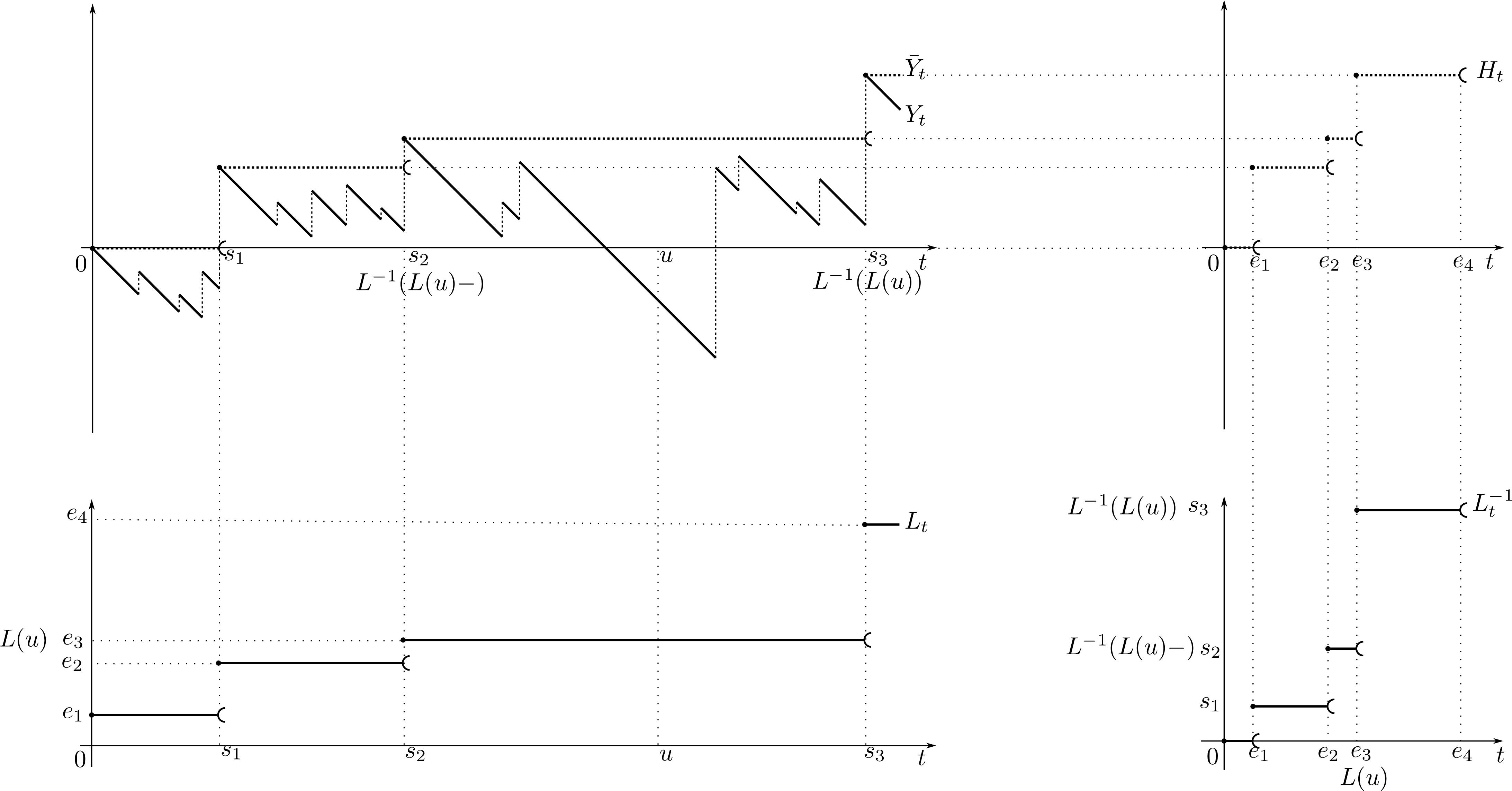
Refer to caption
Figure 6: An example of the paths of ZZ, its local time at the supremum and its ladder process in the finite variation case.

4.3.2 Convergence in distribution of (M)n,εn(M{}_{n,\varepsilon})_{n} towards MεM_{\varepsilon}

The aim of this last subsection is to prove Proposition 4.9, appealing to Theorem 1 in [15]. The four lemmas below ensure that the conditions needed to apply this theorem are fulfilled : First in Lemma 4.22, we make use of Theorem 4.13 to obtain a slightly more precise result about the convergence of the transition measures νm\nu^{\textsc{m}} and νd\nu^{\textsc{d}}. Second, we give in Lemma 4.23 explicit expressions for νn,εinit\nu_{n,\varepsilon}^{\textsc{init}} and νεinit\nu_{\varepsilon}^{\textsc{init}}, which allow us to prove in Lemma 4.24 the weak convergence of νn,εinit\nu_{n,\varepsilon}^{\textsc{init}} towards νεinit\nu_{\varepsilon}^{\textsc{init}}. Finally we deduce from this the convergence in distribution of M(0)n,εM{}_{n,\varepsilon}(0) towards Mε​(0)M_{\varepsilon}(0).

Lemma 4.22.

Suppose xn→xx_{n}\to x as n→∞n\to\infty, where xnx_{n} and xx are positive real numbers. Then νnm​(xn,⋅)\nu^{\textsc{m}}_{n}(x_{n},\cdot) (resp. νnd​(xn,⋅)\nu^{\textsc{d}}_{n}(x_{n},\cdot)) converges weakly towards νm​(x,⋅)\nu^{\textsc{m}}(x,\cdot) (resp. νd​(x,⋅)\nu^{\textsc{d}}(x,\cdot)).

Proof :
Let AA be a set in ℬ⁡([ε,τ)×{0,1})\mathcal{B}([\varepsilon,\tau)\times\{0,1\}) satisfying νm​(x,∂A)=0\nu^{\textsc{m}}(x,\partial A)=0 (where ∂A\partial A denotes the boundary of AA). First write

|νnm​(xn,A)−νm​(x,A)|≤|νnm​(xn,A)−νnm​(x,A)|+|νnm​(x,A)−νm​(x,A)|.|\nu^{\textsc{m}}_{n}(x_{n},A)-\nu^{\textsc{m}}(x,A)|\leq|\nu^{\textsc{m}}_{n}(x_{n},A)-\nu^{\textsc{m}}_{n}(x,A)|+|\nu^{\textsc{m}}_{n}(x,A)-\nu^{\textsc{m}}(x,A)|.

The second term in the right-hand side vanishes thanks to Theorem 4.13. Besides, we have

|ℙ0​(Hn+​(en)∈A,Ln−1​(en)<Tn−xn)−ℙ0​(Hn+​(en)∈A,Ln−1​(en)<T−x)|≤ℙ0​(Tn−x<Tn−xn),|\mathbb{P}_{0}(H^{+}_{n}(\text{e}_{n})\in A,L^{-1}_{n}(\text{e}_{n})<T_{n}^{-x_{n}})-\mathbb{P}_{0}(H^{+}_{n}(\text{e}_{n})\in A,L^{-1}_{n}(\text{e}_{n})<{T^{-x}})|\leq\mathbb{P}_{0}({T_{n}^{-x}}<T_{n}^{-x_{n}}),

which vanishes as n→∞n\to\infty thanks to the a.s. continuity of x↦Tn−xx\mapsto{T_{n}^{-x}} on ℝ+\mathbb{R}_{+} under ℙ0\mathbb{P}_{0}. Then, by definition of νnm\nu^{\textsc{m}}_{n} (see (4)), we get |νnm​(xn,A)−νnm​(x,A)|→0|\nu^{\textsc{m}}_{n}(x_{n},A)-\nu^{\textsc{m}}_{n}(x,A)|\to 0 as n→∞n\to\infty (for the sake of simplicity, we omitted here the conditioning that appears in the definition of νnm\nu^{\textsc{m}}_{n}).

A similar reasoning holds for νd\nu^{\textsc{d}} (the weak convergence of νnd\nu^{\textsc{d}}_{n} towards νd\nu^{\textsc{d}} is a consequence of Lemma 4.17). □\square

Lemma 4.23.

For all (u,q)∈[ε,τ)×{0,1}(u,q)\in[\varepsilon,\tau)\times\{0,1\}, we have

νn,εinit​(d​u,d​q)=(1W~n​(ε)−1W~n​(τ))​W~n​(τ−u)W~n​(τ)​d​u​∫(u,∞)Λ~n​(d​z)​𝔹fn​(n​z)​(d​q)​(1−W~n​(ε−(z−u))W~n​(ε)),\nu_{n,\varepsilon}^{\textsc{init}}(\text{d}u,\text{d}q)\\ =\left(\frac{1}{\tilde{W}_{n}(\varepsilon)}-\frac{1}{\tilde{W}_{n}(\tau)}\right)\frac{\tilde{W}_{n}(\tau-u)}{\tilde{W}_{n}(\tau)}\text{d}u\int_{(u,\infty)}\tilde{\Lambda}_{n}(\text{d}z)\mathbb{B}_{f_{n}(nz)}(\text{d}q)\bigg(1-\frac{\tilde{W}_{n}(\varepsilon-(z-u))}{\tilde{W}_{n}(\varepsilon)}\bigg), (16)
νεinit​(d​u,d​q)=1pε​W⁡(τ−u)W⁡(τ)​[b22​W′​(ε)W⁡(ε)​δε​(d​u)​δ0​(d​q)+d​u​∫(u,∞)Λ⁡(d​z)​𝔹f⁡(z)​(d​q)​(1−W⁡(ε−(z−u))W⁡(ε))],\nu_{\varepsilon}^{\textsc{init}}(\text{d}u,\text{d}q)\\ =\frac{1}{p_{\varepsilon}}\frac{W(\tau-u)}{W(\tau)}\left[\frac{b^{2}}{2}\frac{W^{\prime}(\varepsilon)}{W(\varepsilon)}\delta_{\varepsilon}(\text{d}u)\delta_{0}(\text{d}q)+\text{d}u\int_{(u,\infty)}\Lambda(\text{d}z)\mathbb{B}_{f(z)}(\text{d}q)\bigg(1-\frac{W(\varepsilon-(z-u))}{W(\varepsilon)}\bigg)\right], (17)
Lemma 4.24.

The sequence of measures (νn,εinit)(\nu_{n,\varepsilon}^{\textsc{init}}) converges weakly towards νεinit\nu_{\varepsilon}^{\textsc{init}}.

For the sake of clarity we only prove the two lemmas for νn,εinit​(⋅,{0,1})\nu_{n,\varepsilon}^{\textsc{init}}(\,\cdot\,,\{0,1\}) and νεinit​(⋅,{0,1})\nu_{\varepsilon}^{\textsc{init}}(\,\cdot\,,\{0,1\}).

Proof of Lemma 4.23 :
We begin by proving (16). Recall the following definition :

νn,εinit(⋅,{0,1})=1p′n,εℙ0(Υn∈⋅,Tn−ε<Tn(0,∞)<Tn−τ).\nu_{n,\varepsilon}^{\textsc{init}}(\,\cdot\,,\{0,1\})=\frac{1}{p^{\prime}{}_{n,\varepsilon}}\mathbb{P}_{0}(\Upsilon_{n}\in\,\cdot\,,\ T_{n}^{-\varepsilon}<T_{n}^{(0,\infty)}<T_{n}^{-\tau}).

Applying the strong Markov property at Tn−εT_{n}^{-\varepsilon}, we get :

ℙ0(Υn−ε∈du,Tn−ε<Tn(0,∞)<Tn−τ)=ℙ0(Tn−ε<Tn(0,∞))ℙ−ε(Υn−ε∈du,Tn(0,∞)<Tn−τ).\mathbb{P}_{0}(\Upsilon_{n}-\varepsilon\in\text{d}u,\ T_{n}^{-\varepsilon}<T_{n}^{(0,\infty)}<T_{n}^{-\tau})=\mathbb{P}_{0}(T_{n}^{-\varepsilon}<T_{n}^{(0,\infty)})\mathbb{P}_{-\varepsilon}(\Upsilon_{n}-\varepsilon\in\text{d}u,\ T_{n}^{(0,\infty)}<T_{n}^{-\tau}).

Now conditional on Tn(0,∞)<Tn−τT_{n}^{(0,\infty)}<T_{n}^{-\tau}, Υn−ε\Upsilon_{n}-\varepsilon has the distribution under Nn′(⋅|−infϵ<τ−ε,supϵ≥ε)N^{\prime}_{n}(\cdot\,|\,-\inf\epsilon<\tau-\varepsilon,\ \sup\epsilon\geq\varepsilon) of the undershoot of an excursion at its first entrance time in (0,∞)(0,\infty). Thanks to Proposition 0.5.2(ii) in [3], we then have

ℙ0(Υn−ε∈du,Tn−ε<Tn(0,∞)<Tn−τ)=ℙ0​(Tn−ε<Tn(0,∞))​ℙ−ε​(Tn(0,∞)<Tn−τ)​N′n(−ϵ(χ−)∈du,−infϵ<τ−ε,supϵ≥ε)N′n(−infϵ<τ−ε,supϵ≥ε),\mathbb{P}_{0}(\Upsilon_{n}-\varepsilon\in\text{d}u,\ T_{n}^{-\varepsilon}<T_{n}^{(0,\infty)}<T_{n}^{-\tau})\\ =\mathbb{P}_{0}(T_{n}^{-\varepsilon}<T_{n}^{(0,\infty)})\mathbb{P}_{-\varepsilon}(T_{n}^{(0,\infty)}<T_{n}^{-\tau})\frac{N^{\prime}_{n}(-\epsilon(\chi-)\in\text{d}u,\ -\inf\epsilon<\tau-\varepsilon,\ \sup\epsilon\geq\varepsilon)}{N^{\prime}_{n}(-\inf\epsilon<\tau-\varepsilon,\sup\epsilon\geq\varepsilon)},

Recall that for any ϵ∈ℰ′\epsilon\in\mathscr{E}^{\prime}, χ⁡(ϵ)\chi(\epsilon) denotes the first (and unique) entrance time of ϵ\epsilon into (0,∞)(0,\infty), which is a.s. finite on {−infϵ<τ−ε}\{-\inf\epsilon<\tau-\varepsilon\}.

The process Z~n\tilde{Z}_{n} has finite variation, and it can be shown with elementary calculations that

Nn′(−infϵ<τ−ε,supϵ≥ε)=W~n​(0)W~n​(τ−ε)(W~n​(τ)W~​(ε)−1).N^{\prime}_{n}(-\inf\epsilon<\tau-\varepsilon,\sup\epsilon\geq\varepsilon)=\frac{\tilde{W}_{n}(0)}{\tilde{W}_{n}(\tau-\varepsilon)}\left(\frac{\tilde{W}_{n}(\tau)}{\tilde{W}(\varepsilon)}-1\right).

Along with ℙ0​(Tn−ε<Tn(0,∞))=W~n​(0)W~n​(ε)\mathbb{P}_{0}(T_{n}^{-\varepsilon}<T_{n}^{(0,\infty)})=\frac{\tilde{W}_{n}(0)}{\tilde{W}_{n}(\varepsilon)} and ℙ−ε​(Tn(0,∞)<Tn−τ)=1−W~n​(ε)W~n​(τ)\mathbb{P}_{-\varepsilon}(T_{n}^{(0,\infty)}<T_{n}^{-\tau})=1-\frac{\tilde{W}_{n}(\varepsilon)}{\tilde{W}_{n}(\tau)}, this gives

ℙ0(Υn−ε∈du,Tn−ε<Tn(0,∞)<Tn−τ)\displaystyle\mathbb{P}_{0}(\Upsilon_{n}-\varepsilon\in\text{d}u,\ T_{n}^{-\varepsilon}<T_{n}^{(0,\infty)}<T_{n}^{-\tau})
=\displaystyle= W~n​(τ−ε)W~n​(τ)∫z∈(u,∞)Nn′(−ϵ(χ−)∈du,ϵ(χ)−ϵ(χ−)∈dz,−infϵ<τ−ε,supϵ≥ε)\displaystyle\frac{\tilde{W}_{n}(\tau-\varepsilon)}{\tilde{W}_{n}(\tau)}\ \int_{z\in(u,\infty)}N^{\prime}_{n}(-\epsilon(\chi-)\in\text{d}u,\ \epsilon(\chi)-\epsilon(\chi-)\in\text{d}z,\ -\inf\epsilon<\tau-\varepsilon,\ \sup\epsilon\geq\varepsilon)
=\displaystyle= W~n​(τ−ε)W~n​(τ)​ndn​e−η~n​u​d​u​ℙu​(Tn0<Tn(τ−ε,∞)|Tn0<∞)​∫z∈(u,∞)Λ~n​(d​z)​ℙz−u​(Tn(ε,∞)<Tn0),\displaystyle\frac{\tilde{W}_{n}(\tau-\varepsilon)}{\tilde{W}_{n}(\tau)}\ \frac{n}{d_{n}}e^{-\tilde{\eta}_{n}u}\text{d}u\ \mathbb{P}_{u}(T_{n}^{0}<T_{n}^{(\tau-\varepsilon,\infty)}\,|\,T_{n}^{0}<\infty)\ \int_{z\in(u,\infty)}\tilde{\Lambda}_{n}(\text{d}z)\mathbb{P}_{z-u}(T_{n}^{(\varepsilon,\infty)}<T_{n}^{0}),

where in the last equality we first appealed to the strong Markov property at Tn(0,∞)T_{n}^{(0,\infty)}, and then to Proposition 2.1. Finally, we get

ℙ0(Υn−ε∈du,Tn−ε<Tn(0,∞)<Tn−τ)=ndn​W~n​(τ−u−ε)W~n​(τ)​d​u​∫z∈(u,∞)Λ~n​(d​z)​(1−W~n​(ε−(z−u))W~n​(ε)),\mathbb{P}_{0}(\Upsilon_{n}-\varepsilon\in\text{d}u,\ T_{n}^{-\varepsilon}<T_{n}^{(0,\infty)}<T_{n}^{-\tau})\\ =\frac{n}{d_{n}}\ \frac{\tilde{W}_{n}(\tau-u-\varepsilon)}{\tilde{W}_{n}(\tau)}\ \text{d}u\ \int_{z\in(u,\infty)}\tilde{\Lambda}_{n}(\text{d}z)\left(1-\frac{\tilde{W}_{n}(\varepsilon-(z-u))}{\tilde{W}_{n}(\varepsilon)}\right),

which, along with p′=n,εdnn(1W~n​(ε)−1W~n​(τ))p^{\prime}{}_{n,\varepsilon}=\frac{d_{n}}{n}\left(\frac{1}{\tilde{W}_{n}(\varepsilon)}-\frac{1}{\tilde{W}_{n}(\tau)}\right), proves (16).

We next want to prove (17). A similar reasoning as for (16) holds, except that ZZ has infinite variation. In particular, if ZZ has a Gaussian component, the process can then creep upwards. Using as before the strong Markov property at T−εT^{-\varepsilon} and Proposition 0.5.2(ii) in [3], we have

N′​(ΥCLOSE\displaystyle N^{\prime}(\Upsilon −ε∈du,−infϵ∈[ε,τ))\displaystyle-\varepsilon\in\text{d}u,\ -\inf\epsilon\in[\varepsilon,\tau))
=N′(−infϵ>ε)ℙ−ε(T(0,∞)<T−τ)N′(−ϵ(χ−)∈du,−infϵ<τ−ε,supϵ≥ε)N′(−infϵ<τ−ε,supϵ≥ε).\displaystyle=N^{\prime}(-\inf\epsilon>\varepsilon)\mathbb{P}_{-\varepsilon}(T^{(0,\infty)}<T^{-\tau})\frac{N^{\prime}(-\epsilon(\chi-)\in\text{d}u,\ -\inf\epsilon<\tau-\varepsilon,\ \sup\epsilon\geq\varepsilon)}{N^{\prime}(-\inf\epsilon<\tau-\varepsilon,\ \sup\epsilon\geq\varepsilon)}.

On the one hand, from [22, Section 4] we know that

N′(−infϵ>ε)=1W⁡(ε),\displaystyle N^{\prime}(-\inf\epsilon>\varepsilon)=\frac{1}{W(\varepsilon)},
N′(−infϵ<τ−ε,supϵ≥ε)=1W⁡(τ−ε)(W⁡(τ)W⁡(ε)−1),\displaystyle N^{\prime}(-\inf\epsilon<\tau-\varepsilon,\ \sup\epsilon\geq\varepsilon)=\frac{1}{W(\tau-\varepsilon)}\left(\frac{W(\tau)}{W(\varepsilon)}-1\right),

which gives

ℙ−ε​(T(0,∞)<T−τ)​N′(−infϵ>ε)N′(−infϵ<τ−ε,supϵ≥ε)=(1−W⁡(ε)W⁡(τ))​W⁡(τ−ε)W⁡(τ)−W⁡(ε)=W⁡(τ−ε)W⁡(τ).\mathbb{P}_{-\varepsilon}(T^{(0,\infty)}<T^{-\tau})\frac{N^{\prime}(-\inf\epsilon>\varepsilon)}{N^{\prime}(-\inf\epsilon<\tau-\varepsilon,\ \sup\epsilon\geq\varepsilon)}=\left(1-\frac{W(\varepsilon)}{W(\tau)}\right)\frac{W(\tau-\varepsilon)}{W(\tau)-W(\varepsilon)}=\frac{W(\tau-\varepsilon)}{W(\tau)}.

On the other hand, distinguishing the excursions entering (0,∞)(0,\infty) immediately from the others leads to

N′(−ϵ(χ−)∈du,−infϵ<τ−ε,supϵ≥ε)=N′(−ϵ(χ−)∈du,−infϵ∈(0,τ−ε),supϵ≥ε)+N′(−infϵ=0,supϵ≥ε)δ0(du),N^{\prime}(-\epsilon(\chi-)\in\text{d}u,\ -\inf\epsilon<\tau-\varepsilon,\ \sup\epsilon\geq\varepsilon)\\ =N^{\prime}(-\epsilon(\chi-)\in\text{d}u,\ -\inf\epsilon\in(0,\tau-\varepsilon),\ \sup\epsilon\geq\varepsilon)+N^{\prime}(-\inf\epsilon=0,\ \sup\epsilon\geq\varepsilon)\delta_{0}(\text{d}u),

where N′(−infϵ=0,supϵ≥ε)=b22W′​(ε)W⁡(ε)N^{\prime}(-\inf\epsilon=0,\ \sup\epsilon\geq\varepsilon)=\frac{b^{2}}{2}\frac{W^{\prime}(\varepsilon)}{W(\varepsilon)} according to [22, Section 4].

Then similarly as before, applying the strong Markov property at T(0,∞)T^{(0,\infty)} and Proposition 2.1, we get

N′(Υ−ε∈du,−infϵ∈[ε,τ))\displaystyle N^{\prime}(\Upsilon-\varepsilon\in\text{d}u,\ -\inf\epsilon\in[\varepsilon,\tau))
=W⁡(τ−ε)W⁡(τ)​(e−η~​u​d​u​ℙu​(T0<T(τ−ε,∞)|T0<∞)​∫z∈(u,∞)Λ⁡(d​z)​ℙz−u​(T(ε,∞)<T0)CLOSE\displaystyle=\frac{W(\tau-\varepsilon)}{W(\tau)}\Bigg(e^{-\tilde{\eta}u}\text{d}u\ \mathbb{P}_{u}(T^{0}<T^{(\tau-\varepsilon,\infty)}\,|\,T^{0}<\infty)\ \int_{z\in(u,\infty)}\Lambda(\text{d}z)\mathbb{P}_{z-u}(T^{(\varepsilon,\infty)}<T^{0})
OPEN+b22​W′​(ε)W⁡(ε)​δ0​(d​u))\displaystyle\qquad\qquad\qquad\qquad\qquad\qquad\qquad\qquad\qquad\qquad\qquad\qquad\qquad\qquad\qquad+\frac{b^{2}}{2}\frac{W^{\prime}(\varepsilon)}{W(\varepsilon)}\delta_{0}(\text{d}u)\Bigg)
=W⁡(τ−ε)W⁡(τ)​(b22​W′​(ε)W⁡(ε)​δ0​(d​u)+d​u​W⁡(τ−u)W⁡(τ−ε)​∫z∈(u,∞)Λ⁡(d​z)​(1−W⁡(ε−(z−u))W⁡(ε))),\displaystyle=\frac{W(\tau-\varepsilon)}{W(\tau)}\Bigg(\frac{b^{2}}{2}\frac{W^{\prime}(\varepsilon)}{W(\varepsilon)}\delta_{0}(\text{d}u)+\text{d}u\ \frac{W(\tau-u)}{W(\tau-\varepsilon)}\ \int_{z\in(u,\infty)}\Lambda(\text{d}z)\left(1-\frac{W(\varepsilon-(z-u))}{W(\varepsilon)}\right)\Bigg),

which proves (17). □\square

Proof of Lemma 4.24 :
We can now prove the weak convergence of νn,εinit\nu_{n,\varepsilon}^{\textsc{init}} to νεinit\nu_{\varepsilon}^{\textsc{init}}. To begin with, formulas (16) and (17) of Lemma 4.23, along with the convergence of W~n\tilde{W}_{n} towards WW (which implies in particular p′n,ε→pεp^{\prime}{}_{n,\varepsilon}\to p_{\varepsilon} as n→∞n\to\infty), ensure that we only have to prove the weak convergence of

d​u​ 1u∈(0,τ−ε)​W~n​(τ−u−ε)​∫z∈(u,∞)Λ~n​(d​z)​(1−W~n​(ε−(z−u))W~n​(ε))\text{d}u\ \mathds{1}_{u\in(0,\tau-\varepsilon)}\ \tilde{W}_{n}(\tau-u-\varepsilon)\ \int_{z\in(u,\infty)}\tilde{\Lambda}_{n}(\text{d}z)\left(1-\frac{\tilde{W}_{n}(\varepsilon-(z-u))}{\tilde{W}_{n}(\varepsilon)}\right)

towards

δ0​(d​u)​b22​W′​(ε)W⁡(ε)​W​(τ−ε)+d​u​ 1u∈(0,τ−ε)​W​(τ−u−ε)​∫z∈(u,∞)Λ⁡(d​z)​(1−W⁡(ε−(z−u))W⁡(ε)).\delta_{0}(\text{d}u)\frac{b^{2}}{2}\frac{W^{\prime}(\varepsilon)}{W(\varepsilon)}W(\tau-\varepsilon)+\text{d}u\ \mathds{1}_{u\in(0,\tau-\varepsilon)}\ W(\tau-u-\varepsilon)\ \int_{z\in(u,\infty)}\Lambda(\text{d}z)\left(1-\frac{W(\varepsilon-(z-u))}{W(\varepsilon)}\right).

First notice that since W~n\tilde{W}_{n} and WW vanish on the negative half-line, we have

∫(u,∞)Λ~n(dz)(1−W~n​(ε−(z−u))W~n​(ε))=Λ~¯n(u+ε)+∫(u,u+ε]Λ~n(dz)(1−W~n​(ε−(z−u))W~n​(ε))\displaystyle\int_{(u,\infty)}\tilde{\Lambda}_{n}(\text{d}z)\left(1-\frac{\tilde{W}_{n}(\varepsilon-(z-u))}{\tilde{W}_{n}(\varepsilon)}\right)=\bar{\tilde{\Lambda}}_{n}(u+\varepsilon)+\int_{(u,u+\varepsilon]}\tilde{\Lambda}_{n}(\text{d}z)\left(1-\frac{\tilde{W}_{n}(\varepsilon-(z-u))}{\tilde{W}_{n}(\varepsilon)}\right)
and ∫(u,∞)Λ(dz)(1−W⁡(ε−(z−u))W⁡(ε))=Λ¯(u+ε)+∫(u,u+ε]Λ(dz)(1−W⁡(ε−(z−u))W⁡(ε)).\displaystyle\text{and }\int_{(u,\infty)}\Lambda(\text{d}z)\left(1-\frac{W(\varepsilon-(z-u))}{W(\varepsilon)}\right)=\bar{\Lambda}(u+\varepsilon)+\int_{(u,u+\varepsilon]}\Lambda(\text{d}z)\left(1-\frac{W(\varepsilon-(z-u))}{W(\varepsilon)}\right).

The functions u↦W~n​(τ−u−ε)​Λ~¯n​(u+ε)u\mapsto\tilde{W}_{n}(\tau-u-\varepsilon)\bar{\tilde{\Lambda}}_{n}(u+\varepsilon) converge pointwise on (0,τ−ε)(0,\tau-\varepsilon) towards u↦W⁡(τ−u−ε)​Λ¯​(u+ε)u\mapsto W(\tau-u-\varepsilon)\bar{\Lambda}(u+\varepsilon) and are bounded by supn≥1Λ~¯n​(ε)\sup_{n\geq 1}\bar{\tilde{\Lambda}}_{n}(\varepsilon). Then by dominated convergence, we have the following weak convergence :

d​u​W~n​(τ−u−ε)​Λ~¯n​(u+ε)​𝟙u∈(0,τ−ε)⇒d​u​W​(τ−u−ε)​Λ¯​(u+ε)​𝟙u∈(0,τ−ε).\text{d}u\ \tilde{W}_{n}(\tau-u-\varepsilon)\bar{\tilde{\Lambda}}_{n}(u+\varepsilon)\mathds{1}_{u\in(0,\tau-\varepsilon)}\ \Rightarrow\ \text{d}u\ W(\tau-u-\varepsilon)\bar{\Lambda}(u+\varepsilon)\mathds{1}_{u\in(0,\tau-\varepsilon)}.

Finally, it remains to prove the weak convergence of

du𝟙u∈(0,τ−ε)W~n(τ−u−ε)∫(u,u+ε]Λ~n(dz)(1−W~n​(ε−(z−u))W~n​(ε))\text{d}u\mathds{1}_{u\in(0,\tau-\varepsilon)}\tilde{W}_{n}(\tau-u-\varepsilon)\int_{(u,u+\varepsilon]}\tilde{\Lambda}_{n}(\text{d}z)\left(1-\frac{\tilde{W}_{n}(\varepsilon-(z-u))}{\tilde{W}_{n}(\varepsilon)}\right)

towards

δ0(du)b22W′​(ε)W⁡(ε)W(τ−ε)+du 1u∈(0,τ−ε)W(τ−u−ε)∫z∈(u,u+ε]Λ(dz)(1−W⁡(ε−(z−u))W⁡(ε)).\delta_{0}(\text{d}u)\frac{b^{2}}{2}\frac{W^{\prime}(\varepsilon)}{W(\varepsilon)}W(\tau-\varepsilon)+\text{d}u\ \mathds{1}_{u\in(0,\tau-\varepsilon)}\ W(\tau-u-\varepsilon)\ \int_{z\in(u,u+\varepsilon]}\Lambda(\text{d}z)\left(1-\frac{W(\varepsilon-(z-u))}{W(\varepsilon)}\right).

Consider gg a continuous bounded function on ℝ+\mathbb{R}_{+}. We have :

∫0τ−εdug(u)W~n(τ−u−ε)(∫(u,u+ε]Λ~n(dz)(1−W~n​(ε−(z−u))W~n​(ε)))\displaystyle\int_{0}^{\tau-\varepsilon}\text{d}u\ g(u)\ \tilde{W}_{n}(\tau-u-\varepsilon)\left(\int_{(u,u+\varepsilon]}\tilde{\Lambda}_{n}(\text{d}z)\left(1-\frac{\tilde{W}_{n}(\varepsilon-(z-u))}{\tilde{W}_{n}(\varepsilon)}\right)\right)
=∫(0,τ]Λ~n​(d​z)​(∫0∧z−εzd​u​g​(u)​W~n​(τ−u−ε)​(1−W~n​(ε−(z−u))W~n​(ε)))\displaystyle=\int_{(0,\tau]}\tilde{\Lambda}_{n}(\text{d}z)\left(\int_{0\wedge z-\varepsilon}^{z}\text{d}u\ g(u)\tilde{W}_{n}(\tau-u-\varepsilon)\left(1-\frac{\tilde{W}_{n}(\varepsilon-(z-u))}{\tilde{W}_{n}(\varepsilon)}\right)\right)
=∫(0,τ]Λ~n​(d​z)​(∫0z∧εd​v​g​(z−v)​W~n​(τ−ε−z+v)​(1−W~n​(ε−v)W~n​(ε))).\displaystyle=\int_{(0,\tau]}\tilde{\Lambda}_{n}(\text{d}z)\left(\int_{0}^{z\wedge\varepsilon}\text{d}v\ g(z-v)\tilde{W}_{n}(\tau-\varepsilon-z+v)\left(1-\frac{\tilde{W}_{n}(\varepsilon-v)}{\tilde{W}_{n}(\varepsilon)}\right)\right).

We set, for all u≥0u\geq 0,

hn​(u):=∫0z∧εd​v​g​(z−v)​W~n​(τ−ε−z+v)​(1−W~n​(ε−v)W~n​(ε))h_{n}(u):=\int_{0}^{z\wedge\varepsilon}\text{d}v\ g(z-v)\tilde{W}_{n}(\tau-\varepsilon-z+v)\big(1-\frac{\tilde{W}_{n}(\varepsilon-v)}{\tilde{W}_{n}(\varepsilon)}\big)

h⁡(u):=∫0z∧εd​v​g​(z−v)​W​(τ−ε−z+v)​(1−W⁡(ε−v)W⁡(ε))h(u):=\int_{0}^{z\wedge\varepsilon}\text{d}v\ g(z-v)W(\tau-\varepsilon-z+v)\big(1-\frac{W(\varepsilon-v)}{W(\varepsilon)}\big).

We then verify that the conditions of Proposition 5.2, stated in the appendix, are fulfilled :

  • —

    The functions hnh_{n} and hh can be bounded by ε⋅sup|g|\varepsilon\cdot\sup|g| and are continuous thanks to the continuity on ℝ+\mathbb{R}_{+} of the functions W~n\tilde{W}_{n} and WW.

  • —

    The dominated convergence theorem and the uniform convergence of W~n\tilde{W}_{n} towards WW on ℝ+\mathbb{R}_{+} (see Proposition 4.1.(iii)) ensure that hnh_{n} converges uniformly on ℝ+\mathbb{R}_{+} towards hh (recall that W⁡(ε)>0W(\varepsilon)>0).

  • —

    Now since W~n′\tilde{W}^{\prime}_{n} converges uniformly towards W′W^{\prime} on every compact set of ℝ+∗\mathbb{R}_{+}^{*} (again from Proposition 4.1.(iii)), the sequence (v↦1v​(W~n​(ε)−W~n​(ε−v)))n(v\mapsto\frac{1}{v}(\tilde{W}_{n}(\varepsilon)-\tilde{W}_{n}(\varepsilon-v)))_{n} converges uniformly towards v↦1v​(W~n​(ε)−W~n​(ε−v))v\mapsto\frac{1}{v}(\tilde{W}_{n}(\varepsilon)-\tilde{W}_{n}(\varepsilon-v)) on (0,ε2)(0,\frac{\varepsilon}{2}). Consequently, for all a>0a>0, if nn is large enough we have

    supu∈(0,ε/2)|hn​(u)−h​(u)u2|≤supu∈(0,ε/2)au2​sup|g|​∫0uv​d​v=a2​sup|g|,\sup_{u\in(0,\varepsilon/2)}\left|\frac{h_{n}(u)-h(u)}{u^{2}}\right|\leq\sup_{u\in(0,\varepsilon/2)}\frac{a}{u^{2}}\sup|g|\int_{0}^{u}v\,\text{d}v=\frac{a}{2}\sup|g|,

    and thus we have uniform convergence of u↦hn​(u)/uu\mapsto h_{n}(u)/u towards u↦h⁡(u)/uu\mapsto h(u)/u on (0,ε/2)(0,\varepsilon/2).

  • —

    In the same way we get from the continuity of gg, W~n\tilde{W}_{n} and WW that

    h⁡(u)u2​→u→0​12​g​(ε)​W′​(ε)W⁡(ε)​W​(τ−ε).\frac{h(u)}{u^{2}}\underset{u\to 0}{\to}\frac{1}{2}g(\varepsilon)\frac{W^{\prime}(\varepsilon)}{W(\varepsilon)}W(\tau-\varepsilon).

We then get the expected convergence from an appeal to Proposition 5.2. As a conclusion, we proved that the measures νn,εinit\nu_{n,\varepsilon}^{\textsc{init}} converge weakly to νεinit\nu_{\varepsilon}^{\textsc{init}}. □\square

Lemma 4.25.

As n→∞n\to\infty, M(0)n,εM{}_{n,\varepsilon}(0) converges in distribution towards Mε​(0)M_{\varepsilon}(0).

Proof :
We have to prove the weak convergence of

νn,εinit​(d​u×{1})\nu_{n,\varepsilon}^{\textsc{init}}(\text{d}u\times\{1\}),  ∫[ε,τ)νn,εinit​(d​x×{0})​νnm​(x,d​u)\int_{[\varepsilon,\tau)}\nu_{n,\varepsilon}^{\textsc{init}}(\text{d}x\times\{0\})\nu^{\textsc{m}}_{n}(x,\text{d}u) and  ∫[ε,τ)νn,εinit​(d​x,{0})​νnd​(x,d​u)\int_{[\varepsilon,\tau)}\nu_{n,\varepsilon}^{\textsc{init}}(\text{d}x,\{0\})\nu^{\textsc{d}}_{n}(x,\text{d}u).

The convergence of the first one is a straightforward consequence of Lemma 4.24. We prove below the convergence of the Laplace transform of the second one, and a similar reasoning holds for the third one. We consider for all a≥0a\geq 0

∫(0,∞)e−a​u​∫[ε,τ)νn,εinit​(d​x×{0})​νnm​(x,d​u)=∫[ε,τ)νn,εinit​(d​x×{0})​∫[ε,τ)e−a​u​νnm​(x,d​u)\displaystyle\int_{(0,\infty)}e^{-au}\int_{[\varepsilon,\tau)}\nu_{n,\varepsilon}^{\textsc{init}}(\text{d}x\times\{0\})\nu^{\textsc{m}}_{n}(x,\text{d}u)=\int_{[\varepsilon,\tau)}\nu_{n,\varepsilon}^{\textsc{init}}(\text{d}x\times\{0\})\int_{[\varepsilon,\tau)}e^{-au}\nu^{\textsc{m}}_{n}(x,\text{d}u)

and set hn​(x):=∫[ε,τ)e−a​u​νnm​(x,d​u)h_{n}(x):=\int_{[\varepsilon,\tau)}e^{-au}\nu^{\textsc{m}}_{n}(x,\text{d}u) and h⁡(x):=∫[ε,τ)e−a​u​νm​(x,d​u)h(x):=\int_{[\varepsilon,\tau)}e^{-au}\nu^{\textsc{m}}(x,\text{d}u).

The functions hh and hnh_{n} are all bounded by 11. Moreover, they are continuous : indeed, we have

|𝔼⁡(e−a​H+​(e),L−1​(e)<T−x)−𝔼⁡(e−a​H+​(e),L−1​(e)<T−x0)|≤ℙ⁡(T−x0<T−x),|\mathbb{E}(e^{-aH^{+}(\text{e})},\ L^{-1}(\text{e})<{T^{-x}})-\mathbb{E}(e^{-aH^{+}(\text{e})},\ L^{-1}(\text{e})<T^{-x_{0}})|\leq\mathbb{P}(T^{-x_{0}}<{T^{-x}}),

which vanishes as x→x0x\to x_{0} thanks to the a.s. continuity of x↦T−xx\mapsto{T^{-x}} on ℝ+\mathbb{R}_{+} under ℙ\mathbb{P}. Here again, for the sake of simplicity, we omitted the conditioning, but a similar reasoning and an appeal to the continuity of WW, lead to the continuity of hh. Besides, the same arguments can be used to get the continuity of hnh_{n}. Finally, as established in the proof of [15, Th. 4], Lemma 4.22 ensures the uniform convergence of hnh_{n} towards hh on every compact set of ℝ+∗\mathbb{R}_{+}^{*}. Then, since νn,εinit\nu_{n,\varepsilon}^{\textsc{init}} and νεinit\nu_{\varepsilon}^{\textsc{init}} are probability measures such that νn,εinit⇒νεinit\nu_{n,\varepsilon}^{\textsc{init}}\Rightarrow\nu_{\varepsilon}^{\textsc{init}}, Lemma 5.1 entails the convergence of the Laplace transform of ∫[ε,τ)νn,εinit​(d​x×{0})​νnm​(x,d​u)\int_{[\varepsilon,\tau)}\nu_{n,\varepsilon}^{\textsc{init}}(\text{d}x\times\{0\})\nu^{\textsc{m}}_{n}(x,\text{d}u) towards that of ∫[ε,τ)νεinit​(d​x×{0})​νm​(x,d​u)\int_{[\varepsilon,\tau)}\nu_{\varepsilon}^{\textsc{init}}(\text{d}x\times\{0\})\nu^{\textsc{m}}(x,\text{d}u). □\square

Proof of Proposition 4.9 :
Lemma 4.22 ensures that the Markov chains Mn,εM{}_{n,\varepsilon} and MεM_{\varepsilon} satisfy condition (4).b in [15], while condition (4).a of the same paper is given by Lemma 4.25. Then the announced convergence is a consequence of [15, Theorem (1)]. □\square

5 Appendix

5.1 A convergence lemma for integrals

Lemma 5.1.

Let (hn)n≥0(h_{n})_{n\geq 0} and hh be continuous bounded mappings from ℝd\mathbb{R}^{d} to ℝ\mathbb{R}, and suppose (hn)(h_{n}) is dominated by a bounded function. Let (μn)n≥0(\mu_{n})_{n\geq 0} and μ\mu be in ℳf​(ℝd)\mathcal{M}_{f}(\mathbb{R}^{d}) and suppose that

  1. (i)

    (μn)(\mu_{n}) converges weakly to μ\mu.

  2. (ii)

    The sequence of mappings (hn)(h_{n}) converges to hh uniformly on every compact set of ℝd\mathbb{R}^{d}.

Then

∫hn​d​μn→n→∞∫h​d​μ\int h_{n}\text{d}\mu_{n}\xrightarrow{n\to\infty}\int h\text{d}\mu

Proof :
We have

|∫hn​d​μn−∫h​d​μ|≤|∫(hn−h)​d​(μn−μ)|+|∫(hn−h)​d​μ|+|∫h​d​(μn−μ)|.\left|\int h_{n}\text{d}\mu_{n}-\int h\text{d}\mu\right|\leq\left|\int(h_{n}-h)\text{d}(\mu_{n}-\mu)\right|+\left|\int(h_{n}-h)\text{d}\mu\right|+\left|\int h\text{d}(\mu_{n}-\mu)\right|.

The mapping hh is continuous and bounded on ℝd\mathbb{R}^{d}, then (i) implies the convergence to 00 of the term |∫h​d​(μn−μ)||\int h\text{d}(\mu_{n}-\mu)|. The domination and convergence assumptions made on (hn)(h_{n}) allow us to apply the dominated convergence theorem to get the convergence of |∫(hn−h)​d​μ||\int(h_{n}-h)\text{d}\mu| to 00. As for the first term in the sum, it requires some additional details : Let ε\varepsilon be a positive real number. First, thanks to (i) and since (hn−h)(h_{n}-h) is dominated by a constant, we can find a compact set Kε⊂ℝdK_{\varepsilon}\subset\mathbb{R}^{d} and n0∈ℕn_{0}\in\mathbb{N} such that |∫Kεc(hn−h)​d​(μn−μ)|≤ε|\int_{K_{\varepsilon}^{c}}(h_{n}-h)\text{d}(\mu_{n}-\mu)|\leq\varepsilon for n≥n0n\geq n_{0}. Secondly the uniform convergence on the compact set KεK_{\varepsilon} of the sequence (hn)(h_{n}) ensures that |∫Kε(hn−h)​d​(μn−μ)|≤ε|\int_{K_{\varepsilon}}(h_{n}-h)\text{d}(\mu_{n}-\mu)|\leq\varepsilon for nn large enough. In consequence we have convergence of the term |∫(hn−h)​d​(μn−μ)||\int(h_{n}-h)\text{d}(\mu_{n}-\mu)| to 0, and the result follows. □\square

5.2 Consequences of Assumption A

Then we turn our attention to the proof of Proposition 4.1.

Proof of Proposition 4.1 :

  1. (i)

    Since ZZ is a.s. continuous at T−x{T^{-x}} (resp. is not a compound Poisson process), we have limε→0+​T−(x+ε)=T−x\underset{\varepsilon\to 0+}{\lim}T^{-(x+\varepsilon)}={T^{-x}} (resp.limε→0+​T(y+ε,∞)=T(y,∞)\underset{\varepsilon\to 0+}{\lim}T^{(y+\varepsilon,\infty)}=T^{(y,\infty)}) a.s., and hence the convergence in law of Tn−x{T_{n}^{-x}} towards T−x{T^{-x}} (resp. Tn(y,∞)T_{n}^{(y,\infty)} towards T(y,∞)T^{(y,\infty)}) is a straightforward consequence of Proposition VI.2.11 in [13].

  2. (ii)

    Now ϕn\phi_{n} (resp. ϕ\phi) is the Laplace exponent of the process x↦Tn−xx\mapsto{T_{n}^{-x}} (resp. x↦T−xx\mapsto{T^{-x}}) [3, Th. VII.1.1]. The pointwise convergence of ϕ~n\tilde{\phi}_{n} to ϕ\phi is thus a consequence of point (i). The uniform convergence comes from the fact that for all n≥1n\geq 1, ϕ~n\tilde{\phi}_{n} is increasing on ℝ+\mathbb{R}_{+}.

  3. (iii)

    The proof of the pointwise convergence of W~n\tilde{W}_{n} (resp. W~n′\tilde{W}^{\prime}_{n}) towards WW (resp. W′W^{\prime}) can be found in [19, Prop. 3.1]. Moreover, we have for all y>xy>x ℙ⁡(T−x<T(y−x,∞))=W⁡(x)W⁡(y)\mathbb{P}(T^{-x}<T^{(y-x,\infty)})=\frac{W(x)}{W(y)} [3, Th. VII.2.8], and then the function x↦W~n​(x)/W~n​(y)x\mapsto\tilde{W}_{n}(x)/\tilde{W}_{n}(y) is decreasing, thus the convergence of W~n\tilde{W}_{n} towards WW is uniform on every compact set of ℝ+\mathbb{R}_{+}. Finally, the uniform convergence of W~n′\tilde{W}^{\prime}_{n} towards W′W^{\prime} on every compact set of ℝ+∗\mathbb{R}_{+}^{*} can be deduced from the expression of W~n′\tilde{W}^{\prime}_{n} given in the proof of Lemma 8.2 in [16], as a product of two monotone functions.

□\square

Finally, we recall the following result, obtained in [8] as a consequence of Assumption A.

Proposition 5.2.

Let (gn)n≥0(g_{n})_{n\geq 0} and gg be continuous bounded mappings from ℝ+\mathbb{R}_{+} to ℝ\mathbb{R}, where gg satisfies g⁡(u)/u2→Kg(u)/u^{2}\to K as u→0+u\to 0+ for some constant KK. Assume that the mappings g~n:u↦gn​(u)1∧u2\tilde{g}_{n}:u\mapsto\frac{g_{n}(u)}{1\wedge u^{2}} converge uniformly to g~:u↦g⁡(u)1∧u2\tilde{g}:u\mapsto\frac{g(u)}{1\wedge u^{2}} on ℝ+∗\mathbb{R}_{+}^{*}. Then as n→∞n\to\infty,

Λ~n​(gn)​→n→∞​Λ​(g)+K​b2.\tilde{\Lambda}_{n}(g_{n})\underset{n\to\infty}{\to}\Lambda(g)+Kb^{2}.

References

  • [1] J. Bertoin. Sur la décomposition de la trajectoire d’un processus de Lévy spectralement positif en son infimum. In Annales de l’IHP Probabilités et statistiques, volume 27, pages 537–547. Elsevier, 1991.
  • [2] J. Bertoin. An extension of Pitman’s theorem for spectrally positive Lévy processes. The Annals of Probability, 20(3):1464–1483, 1992.
  • [3] J. Bertoin. Lévy processes, volume 121. Cambridge university press, 1996.
  • [4] J. Bertoin. A limit theorem for trees of alleles in branching processes with rare neutral mutations. Stochastic Processes and their Applications, 120(5):678–697, 2010.
  • [5] N. Champagnat and A. Lambert. Splitting trees with neutral Poissonian mutations I: Small families. Stochastic Processes and their Applications, 122(3):1003–1033, 2012.
  • [6] N. Champagnat and A. Lambert. Splitting trees with neutral Poissonian mutations II: Largest and Oldest families. Stochastic Processes and their Applications, 2012.
  • [7] N. Champagnat, A. Lambert, and M. Richard. Birth and death processes with neutral mutations. International Journal of Stochastic Analysis, 2012, 2012.
  • [8] C. Delaporte. Lévy processes with marked jumps I : Limit theorems. Eprint arXiv:1305.6245.
  • [9] R. Durrett. Probability models for DNA sequence evolution. Springer, 2008.
  • [10] W. J. Ewens. The sampling theory of selectively neutral alleles. Theoretical population biology, 3(1):87–112, 1972.
  • [11] J. Geiger. Size-biased and conditioned random splitting trees. Stochastic processes and their applications, 65(2):187–207, 1996.
  • [12] J. Geiger and G. Kersting. Depth–first search of random trees, and Poisson point processes in Classical and modern branching processes (Minneapolis, 1994) IMA Math. Appl. Vol. 84, 1997.
  • [13] J. Jacod and A.N. Shiryaev. Limit theorems for stochastic processes, volume 288. Springer-Verlag Berlin, 1987.
  • [14] O. Kallenberg. Foundations of modern probability. springer, 2002.
  • [15] A.F. Karr. Weak convergence of a sequence of Markov chains. Probability Theory and Related Fields, 33(1):41–48, 1975.
  • [16] A. Kyprianou. Introductory lectures on fluctuations of Lévy processes with applications. Springer, 2006.
  • [17] A. Lambert. The contour of splitting trees is a Lévy process. The Annals of Probability, 38(1):348–395, 2010.
  • [18] A. Lambert. Species abundance distributions in neutral models with immigration or mutation and general lifetimes. Journal of mathematical biology, 63(1):57–72, 2011.
  • [19] A. Lambert and F. Simatos. Asymptotic behavior of local times of compound Poisson processes with drift in the infinite variance case. arXiv preprint :1206.3800, 2012.
  • [20] J. Lamperti. The limit of a sequence of branching processes. Probability Theory and Related Fields, 7(4):271–288, 1967.
  • [21] M. Nagasawa. Time reversions of Markov processes. Nagoya Mathematical Journal, 24:177–204, 1964.
  • [22] J. Obłój and M. Pistorius. On an explicit Skorokhod embedding for spectrally negative Lévy processes. Journal of Theoretical Probability, 22(2):418–440, 2009.
  • [23] L. Popovic. Asymptotic genealogy of a critical branching process. Annals of Applied Probability, pages 2120–2148, 2004.
  • [24] M. Richard. Splitting trees with neutral mutations at birth. Eprint arXiv:1305.3319.
  • [25] Z. Taïb. Branching processes and neutral evolution. Springer-Verlag, 1992.

*