On multi-time-step monolithic coupling algorithms for elastodynamics

S. Karimi and K. B. Nakshatrala
Department of Civil and Environmental Engineering, University of Houston, Houston, Texas 77204–4003.
Correspondence to: e-mail: knakshatrala@uh.edu, Phone: +1-713-743-4418

Abstract.

We present a way of constructing multi-time-step monolithic coupling methods for elastodynamics. The governing equations for constrained multiple subdomains are written in dual Schur form and enforce the continuity of velocities at system time levels. The resulting equations will be in the form of differential-algebraic equations. To crystallize the ideas we shall employ Newmark family of time-stepping schemes. The proposed method can handle multiple subdomains, and allows different time-steps as well as different time stepping schemes from the Newmark family in different subdomains. We shall use the energy method to assess the numerical stability, and quantify the influence of perturbations under the proposed coupling method. Two different notions of energy preservation are introduced and employed to assess the performance of the proposed method. Several numerical examples are presented to illustrate the accuracy and stability properties of the proposed method. We shall also compare the proposed multi-time-step coupling method with some other methods available in the literature.

Key words and phrases:

monolithic coupling algorithms; multi-time-stepping schemes; subcycling; partitioned schemes; differential-algebraic equations; elastodynamics; Newmark schemes

1. INTRODUCTION AND MOTIVATION

Coupled problems (such as fluid-structure interaction, structure-structure interaction and thermal-structure interaction) have been the subject of intense research in recent years in both computational mechanics and applied mathematics. The report compiled by the Blue Ribbon Panel on Simulation-Based Engineering Science emphasizes that the ability to solve coupled problems will be vital to accelerate the advances in engineering and science through simulation [1]. Developing stable and accurate numerical strategies for coupled problems can be challenging due to several reasons. These problems may involve multiple temporal scales and different spatial scales. One may have to deal with different types of equations for different aspects of physics, which could be coupled nonlinear equations. It is noteworthy that there exists neither a complete mathematical theory (for existence, uniqueness, and sharp estimates) nor a comprehensive computational framework to solve any given coupled problem. Some of the current research efforts are targeted towards resolving the aforementioned issues. Other research efforts are towards developing linear and nonlinear solvers, parallel frameworks, and tools for heterogeneous computing environments (including GPU-based computing) for coupled problems.

Herein, we shall present a numerical approach that can handle moderate disparity in temporal scales. We shall take elastodynamics as the benchmark problem, as it serves two purposes. This problem is important in its own right. In addition, the problem serves as a model problem to develop numerical algorithms for fluid-structure interaction problems, which can be much more involved than a problem typically encountered in elastodynamics. In a fluid-structure interaction simulation, in addition to a coupling algorithm, robust mesh motion algorithms, data transfer algorithms to interpolate data across mismatching meshes, and stable solvers for fluids and solids are needed.

It is now well-recognized that neither implicit nor explicit time-stepping schemes will be totally advantageous to meet all the desired features in a numerical simulation (e.g., see the discussion in references [2, 3]). Many factors (which include mesh, physical properties of the subdomain, accuracy, stability, total time of interest) affect the choice of the time-stepping scheme(s) [4]. It is sometimes much more economical to adopt different time-steps and/or time-stepping schemes in different subdomains. To this end mixed methods and multi-time-step methods have been developed.

1.1. Multi-time-step and mixed methods

Mixed methods refer to a class of algorithms that employ different time-stepping schemes in different subdomains. Some early efforts on mixed methods are [5, 6, 7, 8, 9, 10, 11]. The use of different time-steps in different subdomains is referred to as multi-time-stepping or subcycling. Some representative works in this direction are [12, 13, 14]. But many of the prior efforts on mixed methods and multi-time-stepping suffer from one or more of the following deficiencies: (i) The method cannot handle multiple subdomains. (ii) The method may not be accurate for disparate material properties, and for highly graded meshes. (iii) The method may suffer from very stringent stability limits, which may not be practical to meet realistic problems. (iv) The accuracy and stability depend on the preferential treatment of certain subdomains. For example, in the application of the conventional staggered coupling method, one domain is made to advance before another. The accuracy and stability depends on the choice of the subdomain that has to advance first [15].

We conjecture that the main source of the aforementioned numerical deficiencies is due to the fact that the prior works tried to develop coupling methods for transient problems by extending the strategies that were successful in developing partitioned schemes for static problems. However, it should be emphasized that designing coupling algorithms or partitioned schemes for transient problems require special attention compared to static problems. The governing equations for both undecomposed and decomposed static problems are algebraic equations. In the case of transient problems, the governing equations of an undecomposed problem are Ordinary Differential Equations (ODEs) whereas the governing equations of a decomposed problem are Differential-Algebraic Equations (DAEs).

Many of the prior works just employed the time-stepping schemes that are primarily developed for ODEs to construct partitioned schemes. However, it is well-known in the numerical analysis literature that care should be taken in applying popular time integrating schemes developed for ODEs to solve DAEs. The title of Petzold’s seminal work [16] – “Differential/algebraic equations are not ODEs” – succinctly summarizes this fact. This viewpoint was also taken in references [3, 17] to develop coupling methods for first-order transient systems.

This paper aims to develop a coupling method that allows different time-steps and different time integrators in different parts of the computational domain, which will be achieved using the results from the theory of differential-algebraic equations (e.g., Ascher and Petzold [18]). In recent years, the trend is to use dual Schur approach to develop multi-time-step coupling algorithms for second-order transient systems. A notable work in this direction is by Gravouil and Combescure (e.g., [2], which we shall refer to as the GC method. Based on the GC method, Pegon and Magonette developed a parallel inter-field method (the PM method), reference [19] is devoted to analysis of this method. Bursi et al. extended the PM method by employing the generalized $\alpha$ -method in [20]. Real time partitioned time-integration using the LSRT methods has been of interest recently in [21]. Mahjoubi and Krenk proposed a multi-time-step coupling method using state-pace time integration in [22], a more general presentation of which appears in [23]. Another work that is relevant to the current paper is by Prakash and Hjelmstad [24], which we shall refer to as the PH method. It is worth to critically review the GC and PH methods.

1.1.1. A critical analysis of the GC and PH methods

The GC method is a multi-time-step coupling method for structural problems based on Newmark family of time integrators. The GC coupling method is built based on the following assumptions:

(GC1)

Enforcing the continuity of velocity on the interface at the fine time-steps.
(GC2)

Linear interpolation of interface velocities.
(GC3)

Linear interpolation of Lagrange multiplier within the coarsest time-step.

The GC method is shown to exhibit excessive numerical damping (for example, see reference [24] and the numerical results presented in Section 6 of this paper). The PH method is based on a modification to the GC method, and is constructed based on the following assumptions:

(PH1)

Employed continuity of velocities along the subdomain interface at coarse time-steps.
(PH2)

Linear interpolation of all kinematic variables (displacements, velocities, accelerations of the nodes on the subdomain interface and in the interior of the subdomains) within a coarse time-step.
(PH3)

The method as it is presented in reference [24] is valid only for two subdomains.
(PH4)

The subdomain that has the largest time-step has a more significant role in formulating the algorithm.

In Section 4, we shall show that Assumption (PH2) is not consistent with the underlying physics and need not be consistent with the underlying numerical time-stepping scheme. It is also claimed that the PH method is energy preserving implying that the coupling does not affect the total physical energy of the system. In a subsequent section, we shall present various notions of energy preserving by a coupling algorithm, and show that the PH method is not energy preserving (on the contrary to what has been claimed in Reference [24]).

1.2. Main contributions of this paper

The proposed coupling method is developed by selecting the ideal combination from the assumptions of the GC and PH methods, and thereby eliminating all the deficiencies that these two methods suffer from. This paper has made several advancements in multi-time-step coupling of second-order transient systems, and some of the main ones are as follows:

(i)

Developing a coupling method that can handle multiple subdomains, allows different time-steps in different subdomains, allows different time-stepping schemes under the Newmark family in different subdomains, and is stable and accurate.
(ii)

A stability proof using the energy method to obtain sufficient conditions for multi-time-step coupling is presented. Unlike many of the earlier works, the contribution of interface and subdomains is taken into account to derive the stability criteria. Unlike the prior works on multi-time-step coupling [2, 24], the proof is constructed by taking into account the contributions from all the subdomains and the interface, which is the correct form.
(iii)

Documented the deficiencies of backward difference formulae (BDF) and implicit Runge-Kutta (IRK) schemes (which are popular for solving differential-algebraic equations) for solving second-order transient systems with invariants (e.g., conservation of energy).
(iv)

New notions of energy preservation are introduced and conditions under which the proposed method satisfies any of those notions are also derived.
(v)

A systematic study (both on the theoretical and numerical fronts) on the effect of subcycling and system time-step on the accuracy is presented. Specifically, we have shown that subcycling need not always improve accuracy. A criterion is devised to guide whether subcycling will improve accuracy or not. An attractive feature is that this criterion can be calculated on the fly during a numerical simulation.

1.3. An outline of the paper

The remainder of this paper is organized as follows. Section 2 briefly outlines Newmark family of time stepping schemes. Section 3 presents the governing equations for multiple subdomains with a discussion on the numerical treatment of interface constraints. Section 4 presents the proposed multi-time-step coupling method. A systematic theoretical analysis of the proposed coupling method (which includes stability analysis based on the energy method, influence of perturbations, bounds on interface drifts) is presented in Section 5. In Section 6, some of the theoretical predictions are verified using a simple lumped parameter system. Section 7 discusses the conditions under which the multi-time-step coupling algorithm is energy conserving and the conditions under which it is energy preserving. Some deficiencies of employing backward difference formulae and implicit Runge-Kutta schemes for developing coupling algorithms for elastodynamics are discussed in Section 8. Several representative numerical examples are presented in Section 9 to illustrate the performance of the proposed coupling method. Conclusions are drawn in Section 10.

2. NEWMARK FAMILY OF TIME-STEPPING SCHEMES

Consider a system of second-order ordinary differential equations of the following form:

\displaystyle\boldsymbol{M}\ddot{\boldsymbol{u}}(t)+\boldsymbol{K}\boldsymbol{u}(t)=\boldsymbol{f}(t)\quad t\in(0,T]

(1)

where $t$ denotes time, $T$ denotes the time interval of interest, $\boldsymbol{M}$ is a symmetric positive definite matrix, $\boldsymbol{K}$ is a symmetric positive semidefinite matrix, and a superposed dot denotes derivative with respect to the time. The above system of equations can arise from a semi-discrete finite element discretization of the governing equations in linear elastodynamics [25]. In this case, $\boldsymbol{M}$ is referred to as the mass matrix, $\boldsymbol{K}$ is the stiffness matrix, and $\boldsymbol{u}(t)$ is the nodal displacement vector. Of course, one has to augment the above equation with initial conditions, which, in the context of elastodynamics, will be the prescription of the initial displacement vector and the initial velocity vector. One popular approach for solving equation (1) numerically is to employ a time-stepping scheme from the Newmark family [26]. We now present the Newmark time-stepping schemes in the context of undecomposed problem (i.e., the computational domain is not decomposed into subdomains). In the subsequent sections, we shall extend the presentation to multiple subdomains with the possibility of using different time-steps and/or different time integrators under Newmark family in different subdomains.

Let the time interval of interest $T$ be divided into $N$ sub-intervals such that

\displaystyle[0,T]=\bigcup_{n=1}^{N}[t_{n-1},t_{n}]

(2)

where $0=t_{0}<t_{1}<\cdots<t_{N}=T$ are referred to as time levels. To make the presentation simple, we shall assume that the sub-intervals are uniform. That is,

\displaystyle\Delta t=t_{n}-t_{n-1}\quad\forall n=1,\cdots,N

(3)

where $\Delta t$ is commonly referred to as the time-step. It should be, however, noted that the presentation can be easily extended to incorporate variable time-steps.

Remark 1.

In our development of the proposed multi-time-step coupling method, we shall use different kinds of time-steps (e.g., subdomain time-step, system time-step). These time-steps will be introduced in a subsequent section. For the present discussion, such a distinction is not required, as for single subdomain there is only one time-step.

We shall employ the following notation to denote displacement, velocity and acceleration nodal vectors at discrete time levels:

\displaystyle\boldsymbol{d}^{(n)}=\boldsymbol{u}(t=t_{n}),\quad\boldsymbol{v}^{(n)}=\left.\frac{d\boldsymbol{u}}{dt}\right|_{t=t_{n}},\quad\boldsymbol{a}^{(n)}=\left.\frac{d^{2}\boldsymbol{u}}{dt^{2}}\right|_{t=t_{n}}

(4)

Newmark family of time stepping schemes, which is a two-parameter family of time integrators, can be written as follows:


$\displaystyle\boldsymbol{d}^{(n+1)}$	$\displaystyle=\boldsymbol{d}^{(n)}+\Delta t\;\boldsymbol{v}^{(n)}+\frac{\Delta t^{2}}{2}\left((1-2\beta)\boldsymbol{a}^{(n)}+2\beta\boldsymbol{a}^{(n+1)}\right)$	(5a)
$\displaystyle\boldsymbol{v}^{(n+1)}$	$\displaystyle=\boldsymbol{v}^{(n)}+\Delta t\left((1-\gamma)\boldsymbol{a}^{(n)}+\gamma\boldsymbol{a}^{(n+1)}\right)$	(5b)

where $\beta$ and $\gamma$ are user-specified parameters. A numerical solution at $(n+1)$ -th time level can be obtained by simultaneously solving equations (5a)–(5b) with the following equation:

\displaystyle\boldsymbol{M}\boldsymbol{a}^{(n+1)}+\boldsymbol{K}\boldsymbol{d}^{(n+1)}=\boldsymbol{f}^{(n+1)}

(6)

where

\displaystyle\boldsymbol{f}^{(n+1)}:=\boldsymbol{f}(t=t_{n+1})

(7)

It is well-known that one needs to choose $\gamma\geq 1/2$ for numerical stability [27]. The time-stepping scheme will be unconditionally stable if $2\beta\geq\gamma$ , and will be conditionally stable if $2\beta<\gamma$ . Some popular time-stepping schemes under the Newmark family are the central difference scheme $(\gamma=1/2,\beta=0)$ , the average acceleration scheme $(\gamma=1/2,\beta=1/4)$ , and the linear acceleration scheme $(\gamma=1/2,\beta=1/6)$ . The central difference scheme is also referred to as the velocity Verlet scheme, which is the case in the molecular dynamics literature (e.g., see reference [28]). The central difference scheme is explicit, second-order accurate, and conditionally stable. The average acceleration scheme is implicit, second-order accurate, and unconditionally stable. The linear acceleration scheme is implicit, second-order accurate, and conditionally stable. For further details on Newmark family of time-stepping schemes in the context of undecomposed problem, see references [25, 27, 29].

3. GOVERNING EQUATIONS FOR MULTIPLE SUBDOMAINS

We now write governing equations for multiple subdomains. We will also outline various ways to write subdomain interface conditions, and discuss their pros and cons. To this end, let us divide the domain $\Omega$ into $S$ non-overlapping subdomains, which will be denoted by $\Omega_{1},\cdots,\Omega_{S}$ . That is,

\displaystyle\Omega=\bigcup_{i=1}^{S}\Omega_{i}\quad\mbox{and}\quad\Omega_{i}\cap\Omega_{j}=\emptyset\quad\mbox{for}\;i\neq j

(8)

We shall assume that the meshes in the subdomains are conforming along the subdomain interface, as shown in Figure 1. There are several ways to enforce the continuity along the interface, and hence, several ways to write the governing equations for multiple subdomains. Herein, we shall employ the dual Schur approach [30], which is also employed in the references that are relevant to this paper (i.e., references [2, 24]).

We shall denote the number of displacement degrees-of-freedom in the $i$ -th subdomain by $N_{i}$ . The size of the velocity and acceleration nodal vectors in the $i$ -th subdomain will also be $N_{i}\times 1$ . The interface continuity conditions can be compactly written using signed Boolean matrices. A signed Boolean matrix is a matrix with entries either $0$ , $-1$ , or $+1$ such that each row has at most one non-zero entry. Let us denote the total number of interface constraints by $N_{C}$ . The size of the matrix $\boldsymbol{C}_{i}$ will be $N_{C}\times N_{i}$ .

The governing equations for constrained multiple subdomains in a (time) continuous setting can be written as follows:


		$\displaystyle\boldsymbol{M}_{i}\ddot{\boldsymbol{u}}_{i}(t)+\boldsymbol{K}_{i}\boldsymbol{u}_{i}(t)=\boldsymbol{f}_{i}(t)+\boldsymbol{C}_{i}^{\mathrm{T}}\boldsymbol{\lambda}(t)\quad\forall i=1,\cdots,S$		(9a)
		$\displaystyle\sum_{i=1}^{S}\boldsymbol{C}_{i}\boldsymbol{u}_{i}\left(t\right)=\boldsymbol{0}$		(9b)

where the displacement vector of the $i$ -th subdomain is denoted by $\boldsymbol{u}_{i}\left(t\right)$ , and the external force applied to the $i$ -th subdomain is denoted by $\boldsymbol{f}_{i}(t)$ . The mass and stiffness matrices of the $i$ -th subdomain are denoted by $\boldsymbol{M}_{i}$ and $\boldsymbol{K}_{i}$ respectively. In this paper, we shall assume that the matrices $\boldsymbol{M}_{i}$ are symmetric and positive definite, and the matrices $\boldsymbol{K}_{i}$ to be symmetric and positive semi-definite. Equation (9b) is an algebraic constraint enforcing kinematic continuity of displacements along the subdomain interface. The vector $\boldsymbol{\lambda}$ is the vector of Lagrange multipliers arising due to the enforcement of constraints. The above equations should be augmented with appropriate initial conditions. A brief discussion on the derivation of the above equations can be found in Appendix. Equation (9) form a system of differential-algebraic equations. For the benefit of broader audience, we now briefly discuss differential-algebraic equations.

Remark 2.

If one wants to including physical damping, equation (9a) should be replaced with the following equation:

\displaystyle\boldsymbol{M}_{i}\ddot{\boldsymbol{u}}_{i}(t)+\boldsymbol{D}_{i}\dot{\boldsymbol{u}}_{i}+\boldsymbol{K}_{i}\boldsymbol{u}_{i}(t)=\boldsymbol{f}_{i}(t)+\boldsymbol{C}_{i}^{\mathrm{T}}\boldsymbol{\lambda}(t)\quad\forall i=1,\cdots,S

(10)

where $\boldsymbol{D}_{i}$ is the damping matrix for the $i$ -th subdomain. One can then easily extend the proposed multi-time-step coupling method to include contribution from physical damping. However, a more challenging task is to characterize the performance of the coupling method due to damping. This will depend on several issues like: whether the damping is due to viscoelasticity, plasticity, viscoplasticity or frictional contact? Whether the damping matrix be modeled as Rayleigh damping (which basically assumes that the damping matrix is a linear combination of the mass matrix and the stiffness matrix)? A systematic treatment of these issues are beyond the scope of this paper, and will be addressed in our future works.

3.1. Differential-algebraic equations

A Differential-Algebraic Equation (DAE) is defined as an equation involving unknown functions and their derivatives. A DAE, in its most general form, can be written as follows:

\displaystyle\boldsymbol{g}\left(\dot{\boldsymbol{x}}(t),\boldsymbol{x}(t),t\right)=\boldsymbol{0}\quad t\in(0,T]

(11)

where the unknown function is denoted by $\boldsymbol{x}(t)$ . A DAE of the form given by equation (11) is commonly referred to as an implicit DAE. A quantity that is useful in the study of (smooth) differential-algebraic equations is the so-called differential index, which was first introduced by Gear [31] and further popularized by Petzold and Campbell [18, 32]. For a DAE of the form given by equation (11), differential index is the minimum number of times one has to differentiate with respect to the independent variable $t$ to be able to rewrite equation (11) in the following form:

\displaystyle\dot{\boldsymbol{x}}(t)=\boldsymbol{h}(\boldsymbol{x}(t),t)

(12)

using only algebraic manipulations. It is commonly believed that the higher the differential index the greater will be the difficulty in obtaining stable numerical solutions. An important subclass of DAEs is titled as semi-explicit, which can be written as follows:


	$\displaystyle\dot{\boldsymbol{x}}(t)=\boldsymbol{p}(\boldsymbol{x}(t),t)$		(13a)
	$\displaystyle\boldsymbol{0}=\boldsymbol{q}(\boldsymbol{x}(t),t)$		(13b)

From the above discussion, it is evident that the DAE given by equations (9) is a semi-explicit DAE with differential index 3. One way of solving a higher index DAE is to employ the standard index reduction technique to obtain a mathematically equivalent DAE with lower differential index. It is noteworthy that index reduction can have deleterious effect on the stability and accuracy of numerical solutions (e.g., drift in the constraint). We now explore several mathematically equivalent forms of governing equations, which will have differential index ranging from 0 to 3.

3.2. Subdomain interface constraints

As stated earlier, dual Schur techniques for domain decomposition are of interest throughout this paper. One may write several types of continuity constraints resulting in semi-explicit DAEs of different differential indices. Note that in a continuous setting all these versions are mathematically equivalent. However, from a numerical point of view, their performance can be dramatically different. In fact, some may even exhibit instabilities. Some ways of constructing dual Schur methods are discussed below, which guide future research on constructing new multi-time-step coupling methods.

$\boldsymbol{d}$ -continuity method: This method considers the original set of equations given by equations (9). The method obtains $\left(\boldsymbol{u}_{1}\left(t\right),\cdots,\boldsymbol{u}_{S}\left(t\right),\boldsymbol{\lambda}(t)\right)$ for $t\in(0,T]$ by solving the following equations:


		$\displaystyle\boldsymbol{M}_{i}\ddot{\boldsymbol{u}}_{i}(t)+\boldsymbol{K}_{i}\boldsymbol{u}_{i}(t)=\boldsymbol{f}_{i}(t)+\boldsymbol{C}_{i}^{\mathrm{T}}\boldsymbol{\lambda}\left(t\right)\quad\forall i=1,\cdots,S$		(14a)
		$\displaystyle\sum_{i=1}^{S}\boldsymbol{C}_{i}\boldsymbol{u}_{i}(t)=\boldsymbol{0}$		(14b)

The above equations (14a)–(14b) form a system of DAEs of differential index three. It has been discussed in the literature that the numerical solutions based on this method are prone to instabilities [29, 33].

$\boldsymbol{v}$ -continuity method: This method obtains $\left(\boldsymbol{u}_{1}\left(t\right),\cdots,\boldsymbol{u}_{S}\left(t\right),\boldsymbol{\lambda}(t)\right)$ for $t\in(0,T]$ by solving the following equations:


		$\displaystyle\boldsymbol{M}_{i}\ddot{\boldsymbol{u}}_{i}(t)+\boldsymbol{K}_{i}\boldsymbol{u}_{i}(t)=\boldsymbol{f}_{i}(t)+\boldsymbol{C}_{i}^{\mathrm{T}}\boldsymbol{\lambda}\left(t\right)\quad\forall i=1,\cdots,S$		(15a)
		$\displaystyle\sum_{i=1}^{S}\boldsymbol{C}_{i}\dot{\boldsymbol{u}}_{i}(t)=\boldsymbol{0}$		(15b)

The above equations form a system of DAEs of differential index two. The $\boldsymbol{v}$ -continuity method is of interest in this paper and in the previous works by Gravouil and Combescure [2], and Prakash and Hjelmstad [24]. This form of equations provides a simple but stable framework for seeking numerical solutions, and will form the basis for the proposed multi-time-step coupling method.

$\boldsymbol{a}$ -continuity method: This method obtains $\left(\boldsymbol{u}_{1}\left(t\right),\cdots,\boldsymbol{u}_{S}\left(t\right),\boldsymbol{\lambda}\left(t\right)\right)$ for $t\in(0,T]$ by solving the following equations:


		$\displaystyle\boldsymbol{M}_{i}\ddot{\boldsymbol{u}}_{i}(t)+\boldsymbol{K}_{i}\boldsymbol{u}_{i}(t)=\boldsymbol{f}_{i}(t)+\boldsymbol{C}_{i}^{\mathrm{T}}\boldsymbol{\lambda}\left(t\right)\quad\forall i=1,\cdots,S$		(16a)
		$\displaystyle\sum_{i=1}^{S}\boldsymbol{C}_{i}\ddot{\boldsymbol{u}}_{i}(t)=\boldsymbol{0}$		(16b)

The differential index of the above DAE is unity. A drawback of this method is that there can be significant irrecoverable drift in the displacements without employing constraint stabilization or projection methods. The drift can be attributed to the fact that there is no explicit constraint on the continuity of displacements along the subdomain interface. We, therefore, do not employ this method in this paper.

Baumgarte stabilization method: Under this method, kinematic constraint appears as a linear combination of the kinematic constraints under the $\boldsymbol{d}$ -continuity, $\boldsymbol{v}$ -continuity and $\boldsymbol{a}$ -continuity methods. This method obtains $\left(\boldsymbol{u}_{1}(t),\cdots,\boldsymbol{u}_{S}(t),\boldsymbol{\lambda}(t)\right)$ for $t\in(0,T]$ by solving the following equations:


		$\displaystyle\boldsymbol{M}_{i}\ddot{\boldsymbol{u}}_{i}(t)+\boldsymbol{K}_{i}\boldsymbol{u}_{i}(t)=\boldsymbol{f}_{i}(t)+\boldsymbol{C}_{i}^{\mathrm{T}}\boldsymbol{\lambda}\left(t\right)\quad\forall i=1,\cdots,S$		(17a)
		$\displaystyle\sum_{i=1}^{S}\boldsymbol{C}_{i}\ddot{\boldsymbol{u}}_{i}(t)+\frac{\alpha}{\Delta t}\sum_{i=1}^{S}\boldsymbol{C}_{i}\dot{\boldsymbol{u}}_{i}(t)+\frac{\beta}{\Delta t^{2}}\sum_{i=1}^{S}\boldsymbol{C}_{i}\boldsymbol{u}_{i}(t)=\boldsymbol{0}$		(17b)

where $\alpha$ and $\beta$ are non-dimensional user-specified parameters. One can achieve damping in the drift displacements by choosing parameters satisfying the condition $\alpha^{2}-4\beta<0$ . This method was first proposed by Baumgarte in [34] for constrained mechanical systems. Note that in [34], the coefficients $\alpha$ and $\beta$ have dimensions of $\left[T\right]^{-1}$ and $\left[T\right]^{-2}$ respectively, but in (17), those coefficients are non-dimensionalized. In Reference [17], the Baumgarte stabilization method has been extended to first-order differential-algebraic equations, and the authors were able to derive sufficient conditions for stability using the energy method. To the best of the authors’ knowledge deriving sufficient conditions for stability under the Baumgarte method for second-order differential-algebraic equations is still an open problem. Some notable efforts in this direction are [35, 36, 37].

Rewriting as a system of ordinary differential equations: One can differentiate further, and rewrite the a-continuity method as a system of ordinary differential equations. From the definition of differential index, it is obvious that the differential index of the resulting governing equations will be zero. The governing equations for this method take the following form:


		$\displaystyle\dot{\boldsymbol{u}_{i}}=\boldsymbol{v}_{i}$		(18a)
		$\displaystyle\dot{\boldsymbol{v}}_{i}=\boldsymbol{M}_{i}^{-1}\left(\boldsymbol{f}_{i}+\boldsymbol{C}_{i}^{\mathrm{T}}\boldsymbol{\lambda}-\boldsymbol{K}_{i}\boldsymbol{u}_{i}\right)$		(18b)
		$\displaystyle\boldsymbol{\lambda}=\left(\sum_{i=1}^{S}\boldsymbol{C}_{i}\boldsymbol{M}_{i}^{-1}\boldsymbol{C}_{i}^{\mathrm{T}}\right)^{-1}\left[\sum_{i=1}^{S}\boldsymbol{C}_{i}\boldsymbol{M}_{i}^{-1}\left(\boldsymbol{K}_{i}\boldsymbol{u}_{i}-\boldsymbol{f}_{i}\right)\right]$		(18c)

The main drawback of the above method is that there will be significant irrecoverable drift in the continuity of subdomain interface displacements and velocities. As advocated by Petzold in her famous paper [16], solving DAEs is much harder than solving systems of ODEs. Many of the popular integrators that are used for solving ODEs are not stable and accurate for solving DAEs.

Rewriting as a system of first-order differential-algebraic equations: Yet another approach is to rewrite the governing equations in first-order form, and then employ appropriate time-stepping schemes for solving first-order DAEs (e.g., backward difference formulae, implicit Runge-Kutta schemes). The first-order form can be achieved by introducing an auxiliary variable. The governing equations take the following form:


		$\displaystyle\dot{\boldsymbol{u}}(t)=\boldsymbol{v}(t)$		(19a)
		$\displaystyle\boldsymbol{M}_{i}\dot{\boldsymbol{v}}_{i}+\boldsymbol{K}_{i}\boldsymbol{u}_{i}=\boldsymbol{f}_{i}(t)+\boldsymbol{C}_{i}^{\mathrm{T}}\boldsymbol{\lambda}$		(19b)
		$\displaystyle\sum_{i=1}^{S}\boldsymbol{C}_{i}\boldsymbol{u}_{i}=\boldsymbol{0}$		(19c)

The differential index for the above system is three. If one replaces the interface constraint equation (19c) with either of the following:

\displaystyle\sum_{i=1}^{S}\boldsymbol{C}_{i}\dot{\boldsymbol{u}}_{i}=\boldsymbol{0}\quad\mathrm{or}\quad\sum_{i=1}^{S}\boldsymbol{C}_{i}\boldsymbol{v}_{i}=\boldsymbol{0}

(20)

then the differential index of the resulting differential-algebraic equations will be two. If the interface constraint equation (19c) is replaced with the following:

\displaystyle\sum_{i=1}^{S}\boldsymbol{C}_{i}\dot{\boldsymbol{v}}_{i}=\boldsymbol{0}

(21)

then the resulting first-order DAEs will have index one.

In a subsequent section we shall show that the approach of rewriting the governing equations as first-order DAEs and then employing time-stepping schemes that are typically used for first-order transient systems is not accurate for elastodynamics. Hence, we do not employ such an approach to develop a multi-time-step coupling method. Instead, we consider the governing equations in second-order form and modify Newmark time-stepping schemes to be able to obtain stable and accurate results for resulting DAEs. In the next section, we shall extend the $\boldsymbol{v}$ -continuity to be able to employ different time-steps in different subdomains, and to couple explicit and implicit time-stepping schemes.

4. PROPOSED MULTI-TIME-STEP COUPLING METHOD

The aim of this paper is to solve equations (15a)–(15b) numerically by allowing each subdomain to have its own time-step and its own time integrator from the Newmark family of time stepping schemes. We first introduce notation that will help in presenting the proposed multi-time-step coupling method in a concise manner.

4.1. Notation for multi-time-step coupling

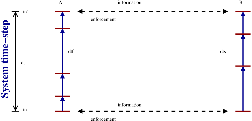
Both the GC and PH methods are devised by introducing the coarsest time-step, which is the maximum of all the subdomain time-steps. This creates bias, at least in the mathematical setting, towards the subdomain that has the maximum time-step. Herein, we alleviate this drawback by introducing the notion of system time-step, which is greater than or equal to the coarsest time-step. Moreover, this approach allows for the possibility of all subdomains to subcycle, which is illustrated in a subsequent section. Figure 2 gives a pictorial description of subdomain time-steps, system time-step, and the concept of subcycling. We shall define $\eta_{i}$ to be the ratio between system time-step ( $\Delta t$ ) and the $i$ -th subdomain time-step ( $\Delta t_{i}$ ). That is,

\displaystyle\eta_{i}:=\frac{\Delta t}{\Delta t_{i}}

(22)

For simplicity, we shall assume that $\eta_{i}$ is a (positive) integer.

We shall use the following notation to represent the value of a quantity of interest at subdomain time levels:

\displaystyle\Box_{i}^{\left(n+\frac{j}{\eta_{i}}\right)}\approx\Box_{i}\left(t=n\Delta t+j\Delta t_{i}\right)

(23)

We shall employ the following notation to group the kinematic quantities:

\displaystyle\boldsymbol{X}_{i}^{\left(n+\frac{j}{\eta_{i}}\right)}:=\left[\begin{array}[]{c}\boldsymbol{a}_{i}^{\left(n+\frac{j}{\eta_{i}}\right)}\\ \boldsymbol{v}_{i}^{\left(n+\frac{j}{\eta_{i}}\right)}\\ \boldsymbol{d}_{i}^{\left(n+\frac{j}{\eta_{i}}\right)}\end{array}\right],\quad\mathbb{X}_{i}^{(n+1)}:=\left[\begin{array}[]{c}\boldsymbol{X}_{i}^{\left(n+\frac{1}{\eta_{i}}\right)}\\ \boldsymbol{X}_{i}^{\left(n+\frac{2}{\eta_{i}}\right)}\\ \vdots\\ \boldsymbol{X}_{i}^{(n+1)}\\ \end{array}\right],\quad\mathbb{X}^{(n+1)}:=\left[\begin{array}[]{c}\mathbb{X}_{1}^{\left(n+1\right)}\\ \mathbb{X}_{2}^{\left(n+1\right)}\\ \vdots\\ \mathbb{X}_{S}^{(n+1)}\\ \end{array}\right]

The vector $\boldsymbol{X}_{i}^{\left(n+\frac{j}{\eta_{i}}\right)}$ contains all the kinematic unknowns for $i$ -th subdomain over its subdomain time-step, $\mathbb{X}_{i}^{(n+1)}$ contains all the kinematic unknowns for $i$ -th subdomain over a system time-step, and the vector $\mathbb{X}^{(n+1)}$ contains the kinematic unknowns of all subdomains over a system time-step. We define the following augmented subdomain signed Boolean matrices:

\displaystyle\mathbb{C}_{i}:=\left[\begin{array}[]{c|c|c|c|c}\underbrace{\mathcal{O}_{i}\quad\mathcal{O}_{i}\quad\mathcal{O}_{i}}_{1}&\underbrace{\mathcal{O}_{i}\quad\mathcal{O}_{i}\quad\mathcal{O}_{i}}_{2}&\cdots\;\cdots\;\cdots&\underbrace{\mathcal{O}_{i}\quad\mathcal{O}_{i}\quad\mathcal{O}_{i}}_{\eta_{i}-1}&\underbrace{\mathcal{O}_{i}\quad\boldsymbol{C}_{i}\quad\mathcal{O}_{i}}_{\eta_{i}}\end{array}\right]

where the matrix $\mathcal{O}_{i}$ contains zeros of the same size as $\boldsymbol{C}_{i}$ (which is $N_{C}\times N_{i}$ ). It is evident that the size of $\mathbb{C}_{i}$ is $N_{C}\times 3\eta_{i}N_{i}$ . The augmented signed Boolean matrix for the entire system is defined as follows:

\displaystyle\mathbb{C}:=\left[\begin{array}[]{cccc}\mathbb{C}_{1}&\mathbb{C}_{2}&\cdots&\mathbb{C}_{S}\end{array}\right]

The size of $\mathbb{C}$ is $N_{C}\times\left(\sum_{i=1}^{S}3\eta_{i}N_{i}\right)$ . The following augmented signed Boolean matrices will be useful in taking into account the effect of interface forces:

\displaystyle\mathbb{B}_{i}^{\mathrm{T}}:=\left[\begin{array}[]{c|c|c|c}-\frac{1}{\eta_{i}}\boldsymbol{C}_{i}\quad\mathcal{O}_{i}\quad\mathcal{O}_{i}&-\frac{2}{\eta_{i}}\boldsymbol{C}_{i}\quad\mathcal{O}_{i}\quad\mathcal{O}_{i}&\cdots\;\cdots\;\cdots&-\frac{\eta_{i}}{\eta_{i}}\boldsymbol{C}_{i}\quad\mathcal{O}_{i}\quad\mathcal{O}_{i}\end{array}\right]

The corresponding signed Boolean matrix for the entire system can be written as follows:

\displaystyle\mathbb{B}:=\left[\begin{array}[]{c}\mathbb{B}_{1}\\ \mathbb{B}_{2}\\ \vdots\\ \mathbb{B}_{S}\end{array}\right]

We shall define the following augmented matrices for each subdomain:

\displaystyle\mathbb{L}_{i}:=\left[\begin{array}[]{ccc}\boldsymbol{M}_{i}&\boldsymbol{O}_{i}&\boldsymbol{K}_{i}\\ -\gamma_{i}\Delta t_{i}\boldsymbol{I}_{i}&\boldsymbol{I}_{i}&\boldsymbol{O}_{i}\\ -\beta_{i}\Delta t_{i}^{2}\boldsymbol{I}_{i}&\boldsymbol{O}_{i}&\boldsymbol{I}_{i}\end{array}\right]\quad\mathbb{R}_{i}:=\left[\begin{array}[]{ccc}\boldsymbol{O}_{i}&\boldsymbol{O}_{i}&\boldsymbol{O}_{i}\\ \left(1-\gamma_{i}\right)\Delta t_{i}\boldsymbol{I}_{i}&\boldsymbol{I}_{i}&\boldsymbol{O}_{i}\\ \left(\frac{1}{2}-\beta_{i}\right)\Delta t_{i}^{2}\boldsymbol{I}_{i}&\Delta t_{i}\boldsymbol{I}_{i}&\boldsymbol{I}_{i}\end{array}\right]

where $\boldsymbol{O}_{i}$ denotes a matrix containing zeros of size $N_{i}\times N_{i}$ , and $\boldsymbol{I}_{i}$ is the identity matrix of size $N_{i}\times N_{i}$ .

4.2. Multi-time-step coupling

The proposed multi-time-step coupling method is developed based on the following assumptions:

(A)

Enforce the continuity of interface velocities at system time-steps.
(B)

The corresponding Lagrange multipliers (which will be interface reactions) are calculated at system time-steps. (It should be noted that the Lagrange multipliers are unknowns,and will be a part of the solution.)
(C)

The Lagrange multipliers are interpolated linearly within system time-steps to approximate their values at subdomain time-steps.
(D)

The equilibrium equations for each subdomain is enforced at its corresponding subdomain time levels.

with a requirement that the coupling method can handle arbitrary number of subdomains.

Assumptions (B) and (C) take the following mathematical form:

\displaystyle\boldsymbol{\lambda}^{\left(n+\frac{j}{\eta_{i}}\right)}=\left(1-\frac{j}{\eta_{i}}\right)\boldsymbol{\lambda}^{\left(n\right)}+\left(\frac{j}{\eta_{i}}\right)\boldsymbol{\lambda}^{\left(n+1\right)}

(48)

where $\boldsymbol{\lambda}^{(n)}$ and $\boldsymbol{\lambda}^{\left(n+1\right)}$ are Lagrange multipliers at system time levels. Using equation (48), Assumption (D) takes the following form:

\displaystyle\boldsymbol{M}_{i}\boldsymbol{a}_{i}^{\left(n+\frac{j+1}{\eta_{i}}\right)}+\boldsymbol{K}_{i}\boldsymbol{d}_{i}^{\left(n+\frac{j+1}{\eta_{i}}\right)}-\frac{j+1}{\eta_{i}}\boldsymbol{C}_{i}^{\mathrm{T}}\left(\boldsymbol{\lambda}^{\left(n+1\right)}-\boldsymbol{\lambda}^{\left(n\right)}\right)=\boldsymbol{f}_{i}^{\left(n+\frac{j+1}{\eta_{i}}\right)}+\boldsymbol{C}_{i}^{\mathrm{T}}\boldsymbol{\lambda}^{\left(n\right)}

(49)

and the relations for the time-stepping schemes for the $i$ -th subdomain take the following form:


		$\displaystyle\boldsymbol{d}_{i}^{\left(n+\frac{j+1}{\eta_{i}}\right)}=\boldsymbol{d}_{i}^{\left(n+\frac{j}{\eta_{i}}\right)}+\Delta t_{i}\boldsymbol{v}_{i}^{\left(n+\frac{j}{\eta_{i}}\right)}+\frac{\left(\Delta t_{i}\right)^{2}}{2}\left(\left(1-2\beta_{i}\right)\boldsymbol{a}_{i}^{\left(n+\frac{j}{\eta_{i}}\right)}+2\beta_{i}\boldsymbol{a}_{i}^{\left(n+\frac{j+1}{\eta_{i}}\right)}\right)$		(50a)
		$\displaystyle\boldsymbol{v}_{i}^{\left(n+\frac{j+1}{\eta_{i}}\right)}=\boldsymbol{v}_{i}^{\left(n+\frac{j}{\eta_{i}}\right)}+\Delta t_{i}\left(\left(1-\gamma_{i}\right)\boldsymbol{a}_{i}^{\left(n+\frac{j}{\eta_{i}}\right)}+\gamma_{i}\boldsymbol{a}_{i}^{\left(n+\frac{j+1}{\eta_{i}}\right)}\right)$		(50b)

where $\beta_{i}$ and $\gamma_{i}$ are the Newmark parameters for the $i$ -th subdomain. Assumption (A) takes the following mathematical form:

\displaystyle\sum_{i=1}^{S}\mathbb{C}_{i}\mathbb{X}_{i}^{\left(n+1\right)}=\boldsymbol{0}

(51)

Or, more compactly,

\displaystyle\mathbb{C}\mathbb{X}^{\left(n+1\right)}=\boldsymbol{0}

(52)

4.2.1. Advance a subdomain over its subdomain time-step

Using the above notation, the governing equations to advance the state of $i$ -th subdomain over its time-step can be compactly written as follows:

\displaystyle\mathbb{L}_{i}\boldsymbol{X}_{i}^{\left(n+\frac{j+1}{\eta_{i}}\right)}-\left(\frac{j+1}{\eta_{i}}\right)\widetilde{\mathbb{C}}_{i}^{\mathrm{T}}\left(\boldsymbol{\lambda}^{\left(n+1\right)}-\boldsymbol{\lambda}^{\left(n\right)}\right)=\mathbb{P}_{i}^{\left(n+\frac{j+1}{\eta_{i}}\right)}+\widetilde{\mathbb{C}}_{i}^{\mathrm{T}}\boldsymbol{\lambda}^{\left(n\right)}+\mathbb{R}_{i}\boldsymbol{X}_{i}^{\left(n+\frac{j}{\eta_{i}}\right)}

(53)

where the following notation has been employed:

\displaystyle\widetilde{\mathbb{C}}_{i}:=\left[\begin{array}[]{ccc}\boldsymbol{C}_{i}&\mathcal{O}_{i}&\mathcal{O}_{i}\end{array}\right]\quad\mathbb{P}_{i}^{\left(n+\frac{j}{\eta_{i}}\right)}:=\left[\begin{array}[]{c}\boldsymbol{f}_{i}^{\left(n+\frac{j}{\eta_{i}}\right)}\\ \boldsymbol{0}\\ \boldsymbol{0}\end{array}\right]

4.2.2. Advance a subdomain over a system time-step

The governing equations to advance a subdomain over a system time-step can be compactly written as follows:

\displaystyle\mathbb{Q}_{i}\mathbb{X}_{i}^{\left(n+1\right)}+\mathbb{B}_{i}\left(\boldsymbol{\lambda}^{\left(n+1\right)}-\boldsymbol{\lambda}^{\left(n\right)}\right)=\mathbb{F}_{i}^{\left(n+1\right)}

(58)

where the matrix $\mathbb{Q}_{i}$ is defined as follows:

\displaystyle\mathbb{Q}_{i}:=\left[\begin{array}[]{c c c c}\mathbb{L}_{i}&&&\\ -\mathbb{R}_{i}&\mathbb{L}_{i}&&\\ &\ddots&\ddots&\\ &&-\mathbb{R}_{i}&\mathbb{L}_{i}\\ \end{array}\right]

4.2.3. Advance all subdomains over a system time-step

We now write the governing equations to advance all the subdomains from (system) time level $t_{n}$ to $t_{n+1}$ (i.e., advance all subdomains by a system time-step) in a compact form. The mathematical statement takes the following form: Find $\mathbb{X}^{(n+1)}$ and $\boldsymbol{\lambda}^{(n+1)}$ by solving the following system of linear equations:

\displaystyle\left[\begin{array}[]{cc}\mathbb{A}&\mathbb{B}\\ \mathbb{C}&\mathbb{O}\end{array}\right]\left[\begin{array}[]{c}\mathbb{X}^{(n+1)}\\ \boldsymbol{\lambda}^{(n+1)}-\boldsymbol{\lambda}^{(n)}\end{array}\right]=\left[\begin{array}[]{c}\mathbb{F}^{(n+1)}\\ \boldsymbol{0}\end{array}\right]

where the matrix $\mathbb{A}$ is defined as follows:

\displaystyle\mathbb{A}:=\left[\begin{array}[]{cccc}\mathbb{Q}_{1}&&&\\ &\mathbb{Q}_{2}&&\\ &&\ddots&\\ &&&\mathbb{Q}_{S}\end{array}\right]

and the following notation is employed:

\displaystyle\mathbb{F}^{(n+1)}:=\left[\begin{array}[]{c}\mathbb{F}_{1}^{(n+1)}\\ \mathbb{F}_{2}^{(n+1)}\\ \vdots\\ \mathbb{F}_{S}^{(n+1)}\end{array}\right]\quad\boldsymbol{\mathbb{F}}_{i}^{(n+1)}:=\left[\begin{array}[]{c}\mathbb{P}_{i}^{\left(n+\frac{1}{\eta_{i}}\right)}+\widetilde{\mathbb{C}}_{i}^{\mathrm{T}}\boldsymbol{\lambda}^{(n)}+\mathbb{R}_{i}\boldsymbol{X}_{i}^{(n)}\\ \mathbb{P}_{i}^{\left(n+\frac{2}{\eta_{i}}\right)}+\widetilde{\mathbb{C}}_{i}^{\mathrm{T}}\boldsymbol{\lambda}^{(n)}\\ \vdots\\ \mathbb{P}_{i}^{(n+1)}+\widetilde{\mathbb{C}}_{i}^{\mathrm{T}}\boldsymbol{\lambda^{(n)}}\end{array}\right]

4.3. Comments on the derivation of the PH method in Reference [24]

One main assumption in deriving the PH method is that the acceleration, velocity and displacement all vary linearly with time within a system time-step. It should be emphasized that such an assumption is not self-consistent. Moreover, this assumption need not be consistent with the underlying time stepping scheme. To wit, the assumption made in deriving the PH method takes the following mathematical form:


		$\displaystyle\boldsymbol{a}_{i}^{\left(n+\frac{j}{\eta_{i}}\right)}=\left(1-\frac{j}{\eta_{i}}\right)\boldsymbol{a}_{i}^{\left(n\right)}+\frac{j}{\eta_{i}}\boldsymbol{a}_{i}^{\left(n+1\right)}$		(81a)
		$\displaystyle\boldsymbol{v}_{i}^{\left(n+\frac{j}{\eta_{i}}\right)}=\left(1-\frac{j}{\eta_{i}}\right)\boldsymbol{v}_{i}^{\left(n\right)}+\frac{j}{\eta_{i}}\boldsymbol{v}_{i}^{\left(n+1\right)}$		(81b)
		$\displaystyle\boldsymbol{d}_{i}^{\left(n+\frac{j}{\eta_{i}}\right)}=\left(1-\frac{j}{\eta_{i}}\right)\boldsymbol{d}_{i}^{\left(n\right)}+\frac{j}{\eta_{i}}\boldsymbol{d}_{i}^{\left(n+1\right)}$		(81c)

Let us consider equation (81a), which can be interpreted as follows:

\displaystyle\boldsymbol{a}_{i}(t)=\boldsymbol{a}_{i}^{\left(n\right)}+\frac{\left(t-t_{n}\right)}{\left(t_{n+1}-t_{n}\right)}\left(\boldsymbol{a}_{i}^{\left(n+1\right)}-\boldsymbol{a}_{i}^{\left(n\right)}\right)\quad t_{n}\leq t\leq t_{n+1}

(82)

If the acceleration varies linearly with the time, the velocity should vary quadratically with the time, and the displacement should vary cubic with the time. Hence, equations (81a)–(81c) are not inherently consistent.

In addition, this assumption need not be consistent with the underlying time stepping scheme, which is typically derived by assuming an ansatz functional form for the variation of the acceleration, velocity or displacement with respect to the time. For example, Newmark average acceleration scheme $(\gamma=1/2,\beta=1/4)$ is constructed by assuming that the acceleration is constant within a time-step [27]. The assumption made in deriving the PH method that the acceleration varies linearly with time within a system time step (i.e., equation (81a) or (82)) will not be consistent if, say, one employs the Newmark average acceleration scheme under the multi-time-step coupling method. More importantly, as shown in the previous section, such a mathematically inconsistent assumption is not warranted to develop a multi-time-step coupling method. Also, the multi-time-step coupling method as presented in Reference [24] is restricted to two subdomains. There is no restriction on the number of subdomains in the proposed multi-time-step coupling method.

Remark 3.

As mentioned earlier, the PH method (as presented in Reference [24]) can handle only two subdomains. Preference is given to the subdomain that has the coarsest time-step. For example, in the final form of the PH method (see [24, equation 43]), the forcing function to advance subdomain $B$ uses $\mathbf{S}_{i}$ , which is based on the quantities of subdomain $A$ . But the forcing function to advance subdomain $A$ does not employ any quantities of subdomain $B$ . Recently, a tree-based approach has been proposed in Reference [38] that combines two subdomains at a time to solve multiple subdomains, which will be computationally intensive. In the case of two subdomains (i.e., $S=2$ ), the proposed coupling method will be same as the PH method if the applied external forces on the subdomain with the coarse time-step is affine with respect to time. The proposed coupling method, however, can handle multiple subdomains, and does not give preference to any subdomain. It should be emphasized that if one wants to implement in a recursive manner using a tree-based approach, the proposed method is amenable.

5. A THEORETICAL ANALYSIS OF THE PROPOSED COUPLING METHOD

5.1. Stability analysis using the energy method

We shall employ the energy method to show the stability of the proposed multi-time-step coupling method. The energy method is a popular strategy employed in Mathematical Analysis to derive estimates and to perform stability analysis. The method is widely employed in the theory of partial differential equations [39], and numerical analysis [40, 25]. The basic idea behind the energy method is to choose an appropriate norm (which is referred to as the energy norm) and show that the solution is bounded under this norm. It should be noted that the energy norm may not correspond to the physical energy.

We shall now introduce the notation that is needed to apply the energy method. The jump and average operators over the system time-step are, respectively, denoted by $\llbracket\cdot\rrbracket$ and $\llangle\cdot\rrangle$ . That is,


$\displaystyle\left\llbracket\boldsymbol{x}^{(n)}\right\rrbracket$	$\displaystyle:=\boldsymbol{x}^{(n+1)}-\boldsymbol{x}^{(n)}$	(83a)
$\displaystyle\left\llangle\boldsymbol{x}^{(n)}\right\rrangle$	$\displaystyle:=\frac{1}{2}\left(\boldsymbol{x}^{(n)}+\boldsymbol{x}^{(n+1)}\right)$	(83b)

The jump and average operators over the subdomain time-step of the $i$ -th subdomain are, respectively, denoted by $\left[\cdot\right]_{i}$ and $\langle\cdot\rangle_{i}$ . That is,


$\displaystyle\left[\boldsymbol{x}^{\left(n+\frac{j}{\eta_{i})}\right)}\right]_{i}$	$\displaystyle:=\boldsymbol{x}^{\left(n+\frac{j+1}{\eta_{i}}\right)}-\boldsymbol{x}^{\left(n+\frac{j}{\eta_{i}}\right)}$	(84a)
$\displaystyle\left\langle\boldsymbol{x}^{\left(n+\frac{j}{\eta_{i}}\right)}\right\rangle_{i}$	$\displaystyle:=\frac{1}{2}\left(\boldsymbol{x}^{\left(n+\frac{j}{\eta_{i}}\right)}+\boldsymbol{x}^{\left(n+\frac{j+1}{\eta_{i}}\right)}\right)$	(84b)

It is easy to show that, for any symmetric matrix $\boldsymbol{S}$ , the jump and average operators obey the following relationship:

\displaystyle\left\llbracket\boldsymbol{x}^{(n)}\right\rrbracket^{\mathrm{T}}\boldsymbol{S}\left\llangle\boldsymbol{x}^{(n)}\right\rrangle=\frac{1}{2}\left\llbracket{\boldsymbol{x}^{(n)}}^{\mathrm{T}}\boldsymbol{S}\boldsymbol{x}^{(n)}\right\rrbracket

(85)

A similar relation holds for $\left[\cdot\right]_{i}$ and $\langle\cdot\rangle_{i}$ . It is important to note that the jump and average operators are linear. That is, for any $\alpha,\beta\in\mathbb{R}$ we have


		$\displaystyle\llbracket\alpha\boldsymbol{x}+\beta\boldsymbol{y}\rrbracket=\alpha\llbracket\boldsymbol{x}\rrbracket+\beta\llbracket\boldsymbol{y}\rrbracket$		(86a)
		$\displaystyle\llangle\alpha\boldsymbol{x}+\beta\boldsymbol{y}\rrangle=\alpha\llangle\boldsymbol{x}\rrangle+\beta\llangle\boldsymbol{y}\rrangle$		(86b)

We shall call a sequence of vectors $\left\{\boldsymbol{x}^{(n)}\right\}_{n=0}^{\infty}$ to be bounded $\forall n$ if there exists a real number $0<M<+\infty$ such that

\displaystyle\left\|\boldsymbol{x}^{(n)}\right\|<M\quad\forall n

(87)

For convenience, we shall use $\boldsymbol{A}_{i}$ to denote

\displaystyle\boldsymbol{A}_{i}:=\boldsymbol{M}_{i}+\left(\Delta t_{i}\right)^{2}\left(\beta_{i}-\frac{\gamma_{i}}{2}\right)\boldsymbol{K}_{i}

(88)

The critical time-step $\Delta t_{i}^{\mathrm{crit}}\geq 0$ in the $i$ -th subdomain is the maximum time-step for which the matrix $\boldsymbol{A}_{i}$ is positive definite. It should be emphasized that $\Delta t_{i}^{\mathrm{crit}}$ is the critical subdomain time-step assuming that there is no coupling between subdomains, which can be easily calculated. Let $\omega_{i}^{\mathrm{max}}$ be the maximum eigenvalue of the generalized eigenvalue problem for the $i$ -th subdomain. That is,

\displaystyle\omega_{i}^{2}\boldsymbol{M}_{i}\boldsymbol{x}_{i}=\boldsymbol{K}_{i}\boldsymbol{x}_{i}

(89)

where $\boldsymbol{x}_{i}$ is the corresponding eigenvector. Then the critical time-step for the $i$ -th subdomain can be written as follows:

\displaystyle\Delta t_{i}^{\mathrm{crit}}=\left\{\begin{array}[]{ll}+\infty&\mbox{for}\;2\beta_{i}\geq\gamma_{i}\geq 1/2\\ \frac{1}{\omega_{i}^{\mathrm{max}}\sqrt{\gamma_{i}/2-\beta_{i}}}&\mbox{for}\;\gamma_{i}\geq 1/2\;\mbox{and}\;\beta_{i}<\gamma_{i}/2\end{array}\right.

We shall choose the subdomain time-step to be smaller than the corresponding critical time-step for the subdomain. That is,

\displaystyle\Delta t_{i}<\Delta t_{i}^{\mathrm{crit}}

(92)

A detailed discussion on the critical time-steps for Newmark family of time integrators can be found in references [25, 27]. For Newmark family of time stepping schemes, it is easy to check the following identities:


		$\displaystyle\left[\boldsymbol{v}_{i}^{\left(n+\frac{j}{\eta_{i}}\right)}\right]_{i}=\Delta t_{i}\left(\left\langle\boldsymbol{a}_{i}^{\left(n+\frac{j}{\eta_{i}}\right)}\right\rangle_{i}+\left(\gamma_{i}-\frac{1}{2}\right)\left[\boldsymbol{a}_{i}^{\left(n+\frac{j}{\eta_{i}}\right)}\right]_{i}\right)$		(93a)
		$\displaystyle\left[\boldsymbol{d}_{i}^{\left(n+\frac{j}{\eta_{i}}\right)}\right]_{i}=\Delta t_{i}\left\langle\boldsymbol{v}_{i}^{\left(n+\frac{j}{\eta_{i}}\right)}\right\rangle_{i}+\Delta t_{i}^{2}\left(\beta_{i}-\frac{\gamma_{i}}{2}\right)\left[\boldsymbol{a}_{i}^{\left(n+\frac{j}{\eta_{i}}\right)}\right]_{i}$		(93b)

Theorem 1.

If $\Delta t_{i}<\Delta t_{i}^{\mathrm{crit}}$ in all subdomains, then the velocity and acceleration vectors for all subdomains are bounded $\forall n$ under the proposed multi-time-step coupling method.

Proof.

Using the governing equation for the $i$ -th subdomain, and the linear interpolation of the Lagrange multiplier, we obtain the following equation:

\displaystyle\boldsymbol{M}_{i}\left[\boldsymbol{a}_{i}^{\left(n+\frac{j}{\eta_{i}}\right)}\right]_{i}+\boldsymbol{K}_{i}\left[\boldsymbol{d}_{i}^{\left(n+\frac{j}{\eta_{i}}\right)}\right]_{i}=\frac{1}{\eta_{i}}\boldsymbol{C}_{i}^{\mathrm{T}}\left\llbracket\boldsymbol{\lambda}^{(n)}\right\rrbracket

(94)

Using equation (93b), the above equation can be rewritten as follows:

\displaystyle\boldsymbol{A}_{i}\left[\boldsymbol{a}_{i}^{\left(n+\frac{j}{\eta_{i}}\right)}\right]_{i}+\Delta t_{i}\boldsymbol{K}_{i}\left\langle\boldsymbol{v}_{i}^{\left(n+\frac{j}{\eta_{i}}\right)}\right\rangle_{i}=\frac{1}{\eta_{i}}\boldsymbol{C}_{i}^{\mathrm{T}}\left\llbracket\boldsymbol{\lambda}^{(n)}\right\rrbracket

(95)

Premultiplying both sides by $\left[\boldsymbol{v}_{i}^{\left(n+\frac{j}{\eta_{i}}\right)}\right]_{i}$ and using equation (93a), we obtain the following equation:

	$\displaystyle\Delta t_{i}\left\langle\boldsymbol{a}_{i}^{\left(n+\frac{j}{\eta_{i}}\right)}\right\rangle_{i}^{\mathrm{T}}\boldsymbol{A}_{i}\left[\boldsymbol{a}_{i}^{\left(n+\frac{j}{\eta_{i}}\right)}\right]_{i}$	$\displaystyle+\Delta t_{i}\left(\gamma_{i}-\frac{1}{2}\right)\left[\boldsymbol{a}_{i}^{\left(n+\frac{j}{\eta_{i}}\right)}\right]_{i}^{\mathrm{T}}\boldsymbol{A}_{i}\left[\boldsymbol{a}_{i}^{\left(n+\frac{j}{\eta_{i}}\right)}\right]_{i}$		(96)
		$\displaystyle+\Delta t_{i}\left[\boldsymbol{v}_{i}^{\left(n+\frac{j}{\eta_{i}}\right)}\right]_{i}^{\mathrm{T}}\boldsymbol{K}_{i}\left\langle\boldsymbol{v}_{i}^{\left(n+\frac{j}{\eta_{i}}\right)}\right\rangle_{i}=\frac{1}{\eta_{i}}\left\llbracket\boldsymbol{\lambda}^{(n)}\right\rrbracket^{\mathrm{T}}\boldsymbol{C}_{i}\left[\boldsymbol{v}_{i}^{\left(n+\frac{j}{\eta_{i}}\right)}\right]_{i}$

Since $\gamma\geq\frac{1}{2}$ and $\boldsymbol{A}_{i}$ is positive definite (as $\Delta t_{i}<\Delta t_{i}^{\mathrm{crit}}$ ), we can conclude that

\displaystyle\Delta t_{i}\left\langle\boldsymbol{a}_{i}^{\left(n+\frac{j}{\eta_{i}}\right)}\right\rangle_{i}^{\mathrm{T}}\boldsymbol{A}_{i}\left[\boldsymbol{a}_{i}^{\left(n+\frac{j}{\eta_{i}}\right)}\right]_{i}+\Delta t_{i}\left[\boldsymbol{v}_{i}^{\left(n+\frac{j}{\eta_{i}}\right)}\right]_{i}^{\mathrm{T}}\boldsymbol{K}_{i}\left\langle\boldsymbol{v}_{i}^{\left(n+\frac{j}{\eta_{i}}\right)}\right\rangle_{i}\leq\frac{1}{\eta_{i}}\left\llbracket\boldsymbol{\lambda}^{(n)}\right\rrbracket^{\mathrm{T}}\boldsymbol{C}_{i}\left[\boldsymbol{v}_{i}^{\left(n+\frac{j}{\eta_{i}}\right)}\right]_{i}

(97)

Noting that $\Delta t=\eta_{i}\Delta t_{i}$ , and the matrices $\boldsymbol{A}_{i}$ and $\boldsymbol{K}_{i}$ are symmetric, we obtain the following:

\displaystyle\frac{\Delta t}{2}\left[{\boldsymbol{a}_{i}^{\left(n+\frac{j}{\eta_{i}}\right)}}^{\mathrm{T}}\boldsymbol{A}_{i}\boldsymbol{a}_{i}^{\left(n+\frac{j}{\eta_{i}}\right)}\right]_{i}+\frac{\Delta t}{2}\left[{\boldsymbol{v}_{i}^{\left(n+\frac{j}{\eta_{i}}\right)}}^{\mathrm{T}}\boldsymbol{K}_{i}\boldsymbol{v}_{i}^{\left(n+\frac{j}{\eta_{i}}\right)}\right]_{i}\leq\left\llbracket\boldsymbol{\lambda}^{(n)}\right\rrbracket^{\mathrm{T}}\boldsymbol{C}_{i}\left[\boldsymbol{v}_{i}^{\left(n+\frac{j}{\eta_{i}}\right)}\right]_{i}

(98)

By summing over $j\;(j=1,\cdots,\eta_{i})$ we obtain the following:

\displaystyle\frac{\Delta t}{2}\left\llbracket{\boldsymbol{a}_{i}^{\left(n\right)}}^{\mathrm{T}}\boldsymbol{A}_{i}\boldsymbol{a}_{i}^{\left(n\right)}+{\boldsymbol{v}_{i}^{\left(n\right)}}^{\mathrm{T}}\boldsymbol{K}_{i}\boldsymbol{v}_{i}^{\left(n\right)}\right\rrbracket\leq{\left\llbracket\lambda^{\left(n\right)}\right\rrbracket}^{\mathrm{T}}\sum_{i=1}^{S}\boldsymbol{C}_{i}\left\llbracket\boldsymbol{v}_{i}^{\left(n\right)}\right\rrbracket

(99)

Summing over $i\;(i=1,\cdots,S)$ and using the continuity of velocities at system time-steps, we obtain the following inequality:

\displaystyle\sum_{i=1}^{S}\left\llbracket{\boldsymbol{a}_{i}^{\left(n\right)}}^{\mathrm{T}}\boldsymbol{A}_{i}\boldsymbol{a}_{i}^{\left(n\right)}+{\boldsymbol{v}_{i}^{\left(n\right)}}^{\mathrm{T}}\boldsymbol{K}_{i}\boldsymbol{v}_{i}^{\left(n\right)}\right\rrbracket\leq 0

(100)

This further implies that

	$\displaystyle\sum_{i=1}^{S}\left({\boldsymbol{a}_{i}^{(n+1)}}^{\mathrm{T}}\boldsymbol{A}_{i}\boldsymbol{a}_{i}^{(n+1)}+{\boldsymbol{v}_{i}^{(n+1)}}^{\mathrm{T}}\boldsymbol{K}_{i}\boldsymbol{v}_{i}^{(n+1)}\right)$	$\displaystyle\leq\sum_{i=1}^{S}\left({\boldsymbol{a}_{i}^{(n)}}^{\mathrm{T}}\boldsymbol{A}_{i}\boldsymbol{a}_{i}^{(n)}+{\boldsymbol{v}_{i}^{(n)}}^{\mathrm{T}}\boldsymbol{K}_{i}\boldsymbol{v}_{i}^{(n)}\right)$
		$\displaystyle\leq...\leq\sum_{i=1}^{S}\left({\boldsymbol{a}_{i}^{(0)}}^{\mathrm{T}}\boldsymbol{A}_{i}\boldsymbol{a}_{i}^{(0)}+{\boldsymbol{v}_{i}^{(0)}}^{\mathrm{T}}\boldsymbol{K}_{i}\boldsymbol{v}_{i}^{(0)}\right)$		(101)

Since the matrices $\boldsymbol{A}_{i}\;(i=1,\cdots,S)$ are positive definite, the matrices $\boldsymbol{K}_{i}\;(i=1,\cdots,S)$ are positive semidefinite, and the vectors $\boldsymbol{v}_{i}^{(0)}$ and $\boldsymbol{a}_{i}^{(0)}$ are bounded, one can conclude that the vectors $\boldsymbol{a}_{i}^{(n)}$ and $\boldsymbol{v}_{i}^{(n)}$ are bounded $\forall n$ and for all subdomains. ∎

Remark 4.

Strictly speaking, in the above proof, one can only conclude that $\boldsymbol{v}_{i}^{(n)}$ are bounded except for vectors that have a component in the null space of $\boldsymbol{K}_{i}$ . This is the case even for the undecomposed case (i.e., no coupling) under the energy method.

5.2. Influence of perturbations under the proposed coupling method

We shall perform the analysis assuming no subcycling. We will follow a procedure similar to the one presented in [41] for differential-algebraic equations. We shall begin with the original system of equations over a (system) time-step:


		$\displaystyle\boldsymbol{M}_{i}\boldsymbol{a}_{i}^{\left(n+1\right)}+\boldsymbol{K}_{i}\boldsymbol{d}_{i}^{\left(n+1\right)}=\boldsymbol{f}_{i}^{\left(n+1\right)}+\boldsymbol{C}_{i}^{\mathrm{T}}\boldsymbol{\lambda}^{\left(n+1\right)}$		(102a)
		$\displaystyle\boldsymbol{v}_{i}^{\left(n+1\right)}=\boldsymbol{v}_{i}^{\left(n\right)}+\Delta t\left(\left(1-\gamma_{i}\right)\boldsymbol{a}_{i}^{\left(n\right)}+\gamma_{i}\boldsymbol{a}_{i}^{\left(n+1\right)}\right)$		(102b)
		$\displaystyle\boldsymbol{d}_{i}^{\left(n+1\right)}=\boldsymbol{d}_{i}^{\left(n\right)}+\Delta t\boldsymbol{v}_{i}^{\left(n\right)}+\frac{\Delta t^{2}}{2}\left(\left(1-2\beta_{i}\right)\boldsymbol{a}_{i}^{\left(n\right)}+2\beta_{i}\boldsymbol{a}_{i}^{\left(n+1\right)}\right)$		(102c)
		$\displaystyle\sum_{i=1}^{S}\boldsymbol{C}_{i}\boldsymbol{v}_{i}^{(n+1)}=\boldsymbol{0}$		(102d)

Now consider the following perturbed system:


		$\displaystyle\boldsymbol{M}_{i}\widehat{\boldsymbol{a}}_{i}^{\left(n+1\right)}+\boldsymbol{K}_{i}\widehat{\boldsymbol{d}_{i}}^{\left(n+1\right)}=\boldsymbol{f}_{i}^{\left(n+1\right)}+\boldsymbol{C}_{i}^{\mathrm{T}}\widehat{\boldsymbol{\lambda}}^{\left(n+1\right)}$		(103a)
		$\displaystyle\widehat{\boldsymbol{v}}_{i}^{\left(n+1\right)}=\widehat{\boldsymbol{v}}_{i}^{\left(n\right)}+\Delta t\left(\left(1-\gamma_{i}\right)\widehat{\boldsymbol{a}}_{i}^{\left(n\right)}+\gamma_{i}\widehat{\boldsymbol{a}}_{i}^{\left(n+1\right)}\right)+\Delta t\boldsymbol{\varepsilon}_{v_{i}}$		(103b)
		$\displaystyle\widehat{\boldsymbol{d}}_{i}^{\left(n+1\right)}=\widehat{\boldsymbol{d}}_{i}^{\left(n\right)}+\Delta t\widehat{\boldsymbol{v}}_{i}^{\left(n\right)}+\frac{\Delta t^{2}}{2}\left(\left(1-2\beta_{i}\right)\widehat{\boldsymbol{a}}_{i}^{\left(n\right)}+2\beta_{i}\widehat{\boldsymbol{a}}_{i}^{\left(n+1\right)}\right)+\Delta t^{2}\boldsymbol{\varepsilon}_{d_{i}}$		(103c)
		$\displaystyle\sum_{i=1}^{S}\boldsymbol{C}_{i}\widehat{\boldsymbol{v}}_{i}^{(n+1)}=\boldsymbol{\varepsilon}_{\lambda}$		(103d)

where $\boldsymbol{\varepsilon}_{v_{i}}$ , $\boldsymbol{\varepsilon}_{d_{i}}$ and $\boldsymbol{\varepsilon}_{\lambda}$ are, respectively, the perturbations to the original system of equations (102a)–(102d). The solution to this perturbed system of equations will be $\widehat{\boldsymbol{a}}_{i}^{(n+1)}$ , $\widehat{\boldsymbol{v}}_{i}^{(n+1)}$ , $\widehat{\boldsymbol{d}}_{i}^{(n+1)}$ and $\widehat{\boldsymbol{\lambda}}^{(n+1)}$ . For convenience, we shall define the following quantities:


		$\displaystyle\delta\boldsymbol{a}_{i}^{(n+1)}:=\widehat{\boldsymbol{a}}_{i}^{(n+1)}-\boldsymbol{a}_{i}^{(n+1)}$		(104a)
		$\displaystyle\delta\boldsymbol{v}_{i}^{(n+1)}:=\widehat{\boldsymbol{v}}_{i}^{(n+1)}-\boldsymbol{v}_{i}^{(n+1)}$		(104b)
		$\displaystyle\delta\boldsymbol{d}_{i}^{(n+1)}:=\widehat{\boldsymbol{d}}_{i}^{(n+1)}-\boldsymbol{d}_{i}^{(n+1)}$		(104c)
		$\displaystyle\delta\boldsymbol{\lambda}^{(n+1)}:=\widehat{\boldsymbol{\lambda}}^{(n+1)}-\boldsymbol{\lambda}^{(n+1)}$		(104d)

By subtracting equation (102a) from equation (103a) we obtain the following:

\displaystyle\boldsymbol{M}_{i}\delta\boldsymbol{a}_{i}^{\left(n+1\right)}+\boldsymbol{K}_{i}\delta\boldsymbol{d}_{i}^{\left(n+1\right)}=\boldsymbol{C}_{i}^{\mathrm{T}}\delta\boldsymbol{\lambda}^{\left(n+1\right)}

(105)

Using equations (102c) and (103c), the above equation can be written as follows:

\displaystyle\delta\boldsymbol{a}_{i}^{(n+1)}+\boldsymbol{B}_{i}^{-1}\boldsymbol{K}_{i}\left(\delta\boldsymbol{d}_{i}^{(n)}+\Delta t\delta\boldsymbol{v}_{i}^{(n)}+\Delta t^{2}(1/2-\beta_{i})\delta\boldsymbol{a}_{i}^{(n)}\right)=\boldsymbol{B}_{i}^{-1}\boldsymbol{C}_{i}^{\mathrm{T}}\delta\boldsymbol{\lambda}^{(n+1)}-\Delta t^{2}\boldsymbol{B}_{i}^{-1}\boldsymbol{K}_{i}\boldsymbol{\varepsilon}_{d_{i}}

(106)

where the matrix $\boldsymbol{B}_{i}$ has been defined as follows:

\displaystyle\boldsymbol{B}_{i}:=\boldsymbol{M}_{i}+\beta_{i}\Delta t^{2}\boldsymbol{K}_{i}

(107)

The operation $\boldsymbol{B}_{i}^{-1}$ in equation (106) is justified as the matrix is positive definite and hence invertible. By multiplying both sides of equation (106) by $\gamma_{i}\Delta t$ and using equations (102b) and (103b), one can arrive at the following equation:

	$\displaystyle\delta\boldsymbol{v}_{i}^{(n+1)}-\delta\boldsymbol{v}_{i}^{(n)}$	$\displaystyle-(1-\gamma_{i})\Delta t\delta\boldsymbol{a}_{i}^{(n)}-\Delta t\boldsymbol{\varepsilon}_{v_{i}}+\gamma_{i}\Delta t\boldsymbol{B}_{i}^{-1}\boldsymbol{K}_{i}\left(\delta\boldsymbol{d}_{i}^{(n)}+\Delta t\delta\boldsymbol{v}_{i}^{(n)}+\Delta t^{2}(1/2-\beta_{i})\delta\boldsymbol{a}_{i}^{(n)}\right)$
		$\displaystyle=\gamma_{i}\Delta t\boldsymbol{B}_{i}^{-1}\boldsymbol{C}_{i}^{\mathrm{T}}\delta\boldsymbol{\lambda}^{(n+1)}-\gamma_{i}\Delta t^{3}\boldsymbol{B}_{i}^{-1}\boldsymbol{K}_{i}\boldsymbol{\varepsilon}_{d_{i}}$		(108)

We shall assume that $\sum_{i=1}^{S}\boldsymbol{C}_{i}\delta\boldsymbol{v}_{i}^{(n)}=\boldsymbol{0}$ . That is, the constraint is exactly satisfied at the $n$ -th time level. Premultiplying both sides by $\boldsymbol{C}_{i}$ , summing over $i$ (i.e., the number of subdomains), and using equations (102d) and (103d); one can arrive at the following equation:

	$\displaystyle\boldsymbol{\varepsilon}_{\lambda}-\Delta t\sum_{i=1}^{S}(1-\gamma_{i})\boldsymbol{C}_{i}\delta\boldsymbol{a}_{i}^{(n)}$	$\displaystyle-\Delta t\sum_{i=1}^{S}\boldsymbol{C}_{i}\boldsymbol{\varepsilon}_{v_{i}}+\Delta t\sum_{i=1}^{S}\gamma_{i}\boldsymbol{C}_{i}\boldsymbol{B}_{i}^{-1}\boldsymbol{K}_{i}\left(\delta\boldsymbol{d}_{i}^{(n)}+\Delta t\delta\boldsymbol{v}_{i}^{(n)}+\Delta t^{2}(1/2-\beta_{i})\delta\boldsymbol{a}_{i}^{(n)}\right)$
		$\displaystyle=\Delta t\left(\sum_{i=1}^{S}\gamma_{i}\boldsymbol{C}_{i}\boldsymbol{B}_{i}^{-1}\boldsymbol{C}_{i}^{\mathrm{T}}\right)\delta\boldsymbol{\lambda}^{(n+1)}-\Delta t^{3}\sum_{i=1}^{S}\gamma_{i}\boldsymbol{C}_{i}\boldsymbol{B}_{i}^{-1}\boldsymbol{K}_{i}\boldsymbol{\varepsilon}_{d_{i}}$		(109)

By taking norm on both sides and invoking triangle inequality, one can arrive at the following estimate for $\delta\boldsymbol{\lambda}^{(n+1)}$ :

\displaystyle\|\delta\boldsymbol{\lambda}^{(n+1)}\|\leq C_{\lambda}\left(\frac{1}{\Delta t}\|\boldsymbol{\varepsilon}_{\lambda}\|+\sum_{i=1}^{S}\left(\|\boldsymbol{\varepsilon}_{v_{i}}\|+\Delta t^{2}\|\boldsymbol{\varepsilon}_{d_{i}}\|+\|\delta\boldsymbol{a}_{i}^{(n)}\|+\Delta t\|\delta\boldsymbol{v}_{i}^{(n)}\|+\|\delta\boldsymbol{d}_{i}^{(n)}\|\right)\right)

(110)

where $C_{\lambda}$ is a constant. Following a similar procedure for displacements, velocities, and accelerations we obtain the following:

		$\displaystyle\\|\delta\boldsymbol{d}_{i}^{\left(n+1\right)}\\|\leq C_{d}\left(\\|\delta\boldsymbol{d}_{i}^{(n)}\\|+\Delta t\\|\delta\boldsymbol{v}_{i}^{(n)}\\|+\Delta t^{2}\\|\boldsymbol{\varepsilon}_{d_{i}}\\|+\Delta t\\|\boldsymbol{\varepsilon}_{\lambda}\\|+\sum_{i=1}^{S}\left(\Delta t^{2}\\|\delta\boldsymbol{a}_{i}^{(n)}\\|+\Delta t\\|\boldsymbol{\varepsilon}_{v_{i}}\\|\right)\right)$		(111)
		$\displaystyle\\|\delta\boldsymbol{v}_{i}^{\left(n+1\right)}\\|\leq C_{v}\left(\\|\delta\boldsymbol{v}_{i}^{(n)}\\|+\\|\boldsymbol{\varepsilon}_{\lambda}\\|+\sum_{i=1}^{S}\left(\Delta t\\|\delta\boldsymbol{a}_{i}^{(n)}\\|+\Delta t\\|\delta\boldsymbol{d}_{i}^{(n)}\\|+\Delta t^{3}\\|\boldsymbol{\varepsilon}_{d_{i}}\\|+\Delta t\\|\boldsymbol{\varepsilon}_{v_{i}}\\|\right)\right)$		(112)
		$\displaystyle\\|\delta\boldsymbol{a}_{i}^{\left(n+1\right)}\\|\leq C_{a}\left(\frac{1}{\Delta t}\\|\boldsymbol{\varepsilon}_{\lambda}\\|+\Delta t\\|\delta\boldsymbol{v}_{i}^{(n)}\\|+\sum_{i=1}^{S}\left(\\|\delta\boldsymbol{a}_{i}^{(n)}\\|+\\|\delta\boldsymbol{d}_{i}^{(n)}\\|+\Delta t^{2}\\|\boldsymbol{\varepsilon}_{d_{i}}\\|+\\|\boldsymbol{\varepsilon}_{v_{i}}\\|\right)\right)$		(113)

where $C_{d}$ , $C_{v}$ and $C_{a}$ are constants. From the above estimate (110), one can see that a perturbation in the constraint, $\boldsymbol{\varepsilon}_{\lambda}$ , leads to an amplification by $1/\Delta t$ in the Lagrange multiplier. On the other hand, the perturbations in the variables $\boldsymbol{d}_{i}$ and $\boldsymbol{v}_{i}$ lead to (at most) linear growth in the Lagrange multiplier. Clearly, the estimate for the proposed coupling method under no subcycling follows the typical behavior of differential-algebraic equations. An extension of this study to include subcycling will require a more involved and careful analysis, and is beyond the scope of this paper.

5.3. On drifts in interface displacement and acceleration vectors

In a time continuous setting, enforcing the continuity of either displacements, velocities or accelerations are all mathematically equivalent. However, in a numerical setting this equivalence will not hold, and the numerical performance will depend on the type of the constraint that is being enforced. As mentioned in the previous sections, we employ the continuity of velocities at the subdomain interface at every system time-step (which we referred to as the $\boldsymbol{v}$ -continuity). This may lead to drift in the displacements and the accelerations along the subdomain interface. We now derive bounds on these drifts, which could serve as a valuable check for the correctness of a numerical implementation.

For the present study, we shall assume that there is no subcycling (i.e., $\eta_{i}=1$ ), and no mixed methods are employed (i.e., $\beta_{i}=\beta$ , $\gamma_{i}=\gamma$ ). The errors due to finite precision arithmetic and their numerical propagation are ignored. For convenience, let us denote the drift in the displacements and the drift in the accelerations along the subdomain interface as follows:


	$\displaystyle\boldsymbol{a}_{\mathrm{drift}}^{(n)}:=\sum_{i=1}^{S}\boldsymbol{C}_{i}\boldsymbol{a}_{i}^{(n)}$		(114a)
	$\displaystyle\boldsymbol{d}_{\mathrm{drift}}^{(n)}:=\sum_{i=1}^{S}\boldsymbol{C}_{i}\boldsymbol{d}_{i}^{(n)}$		(114b)

Basically, the drift in displacements (or accelerations) is the measure of error in meeting the continuity of displacements (or accelerations) across the subdomain interface. The drifts satisfy the following relations:


$\displaystyle\boldsymbol{a}_{\mathrm{drift}}^{(n+1)}$	$\displaystyle=\left(1-\frac{1}{\gamma}\right)\boldsymbol{a}_{\mathrm{drift}}^{(n)}$	(115a)
$\displaystyle\boldsymbol{d}_{\mathrm{drift}}^{(n+1)}$	$\displaystyle=\boldsymbol{d}_{\mathrm{drift}}^{(n)}+\left(\frac{1}{2}-\frac{\beta}{\gamma}\right)\Delta t^{2}\boldsymbol{a}_{\mathrm{drift}}^{(n)}$	(115b)

Thus, one can draw the following conclusions about the drifts:

(i)

For numerical stability of a time-stepping scheme under Newmark family, $\gamma\geq 1/2$ . Therefore,

$\displaystyle\|\boldsymbol{a}_{\mathrm{drift}}^{(n+1)}\|\leq\|\boldsymbol{a}_{\mathrm{drift}}^{(n)}\|$ (116)

One has the equality only when $\gamma=1/2$ (e.g., Newmark average acceleration scheme, central difference scheme, Newmark linear acceleration scheme).
(ii)

For any time stepping scheme with $\gamma=2\beta$ (e.g., Newmark average acceleration scheme) we have

$\displaystyle\boldsymbol{d}_{\mathrm{drift}}^{(n+1)}=\boldsymbol{d}_{\mathrm{drift}}^{(n)}\quad n=1,2,\cdots$ (117)

The above claims will be numerically substantiated in a subsequent section using the test problem outlined in subsection 9.3.

6. SPLIT DEGREE-OF-FREEDOM LUMPED PARAMETER SYSTEM

Consider a split agree of freedom whose motion can be described by the following system of ordinary differential/algebraic equation:


		$\displaystyle m_{A}\ddot{u}_{A}(t)+k_{A}u_{A}(t)=f_{A}(t)+\lambda(t)$		(118a)
		$\displaystyle m_{B}\ddot{u}_{B}(t)+k_{B}u_{B}(t)=f_{B}(t)-\lambda(t)$		(118b)
		$\displaystyle\dot{u}_{A}(t)-\dot{u}_{B}(t)=0$		(118c)

The following parameters are used: $m_{A}=0.1$ , $m_{B}=0.005$ , and the stiffness of springs are $k_{A}=2.5$ and $k_{B}=50$ . The subdomain time-steps are taken as $\Delta t_{A}=0.02$ and $\Delta t_{B}=0.005$ . The system time-step is taken as $\Delta t=0.02$ . The values of the external forces are taken to be zero, that is $f_{A}=0$ and $f_{B}=0$ . The initial conditions are $d_{0}=0.1$ and $v_{0}=1.0$ . The problem is solved over a time interval of $[0,0.5]$ . In all the cases, Newmark average acceleration scheme is used in all the subdomains. The resulting numerical results for kinematic variables are shown in Figure 4. Since the external forces applied are constant ( $f_{A}=f_{B}=0$ ) the PH method and the proposed coupling methods yield the same results. The GC method suffers from excessive damping and fails to match the exact results. Similar observation can be made about the interface force as well as total physical energy of the system, as shown in Figure 5.

7. ON ENERGY CONSERVING VS. ENERGY PRESERVING COUPLING

In this section we address the energy preserving and energy conserving properties of the proposed multi-time-step coupling method. Two different notions of energy preserving will be considered. In particular, the following questions will be answered:

(a)

Does the coupling method add or extract energy from the system of subdomains in comparison with the case of no coupling?
(b)

Do the interface forces perform net work?
(c)

Under what conditions does the coupling method conserve the total energy of the system of subdomains?

To this end, the kinetic energy and the potential energy of the $i$ -th subdomain are, respectively, defined as follows:

\displaystyle\mathcal{T}_{i}\left(\boldsymbol{v}_{i}\right):=\frac{1}{2}\boldsymbol{v}_{i}^{\mathrm{T}}\boldsymbol{M}_{i}\boldsymbol{v}_{i}\quad\mathcal{V}_{i}\left(\boldsymbol{d}_{i}\right):=\frac{1}{2}\boldsymbol{d}_{i}^{\mathrm{T}}\boldsymbol{K}_{i}\boldsymbol{d}_{i}

(119)

The total energy of the $i$ -th subdomain is given by

\displaystyle\mathcal{E}_{i}\left(\boldsymbol{d}_{i},\boldsymbol{v}_{i}\right):=\mathcal{T}_{i}\left(\boldsymbol{v}_{i}\right)+\mathcal{V}_{i}\left(\boldsymbol{d}_{i}\right)

(120)

The total energy of all the subdomains at the $n$ -th (system) time level can be written as follows:

\displaystyle\mathcal{E}^{(n)}\equiv\mathcal{E}\left(\boldsymbol{d}_{1}^{(n)},\cdots,\boldsymbol{d}_{S}^{(n)},\boldsymbol{v}_{1}^{(n)},\cdots,\boldsymbol{v}_{S}^{(n)}\right):=\sum_{i=1}^{S}\mathcal{E}_{i}\left(\boldsymbol{d}_{i}^{(n)},\boldsymbol{v}_{i}^{(n)}\right)

(121)

In the remainder of this section, we shall assume that the external forces are zero (i.e., $\boldsymbol{f}_{i}(t)=\boldsymbol{0}\;\forall i$ ). For the proposed multi-time-step method, one can derive the following relationship:

\displaystyle\mathcal{E}^{(n+1)}-\mathcal{E}^{(n)}=\mathcal{E}^{(n\rightarrow n+1)}_{\mathrm{algorithm}}+\mathcal{E}^{(n\rightarrow n+1)}_{\mathrm{interface}}

(122)

where $\mathcal{E}_{\mathrm{algorithm}}^{(n\rightarrow n+1)}$ and $\mathcal{E}_{\mathrm{interface}}^{(n\rightarrow n+1)}$ are, respectively, defined as follows:

$\displaystyle\mathcal{E}^{(n\rightarrow n+1)}_{\mathrm{algorithm}}$	$\displaystyle:=-2\sum_{i=1}^{S}\sum_{j=0}^{\eta_{i}-1}\left(\gamma_{i}-\frac{1}{2}\right)\mathcal{V}_{i}\left(\left[\boldsymbol{d}_{i}^{\left(n+\frac{j}{\eta_{i}}\right)}\right]_{i}\right)-\Delta t^{2}\sum_{i=1}^{S}\frac{1}{\eta_{i}^{2}}\left(\beta_{i}-\frac{\gamma_{i}}{2}\right)\left\llbracket\mathcal{T}_{i}\left(\boldsymbol{a}_{i}^{(n)}\right)\right\rrbracket$
	$\displaystyle-\Delta t^{2}\sum_{i=1}^{S}\frac{1}{\eta_{i}^{2}}\left(\beta_{i}-\frac{\gamma_{i}}{2}\right)\left(2\gamma_{i}-1\right)\left(\sum_{j=0}^{\eta_{i}-1}\mathcal{T}_{i}\left(\left[\boldsymbol{a}_{i}^{\left(n+\frac{j}{\eta_{i}}\right)}\right]_{i}\right)\right)$	(123)
$\displaystyle\mathcal{E}_{\mathrm{interface}}^{(n\rightarrow n+1)}$	$\displaystyle:=\sum_{i=1}^{S}\sum_{j=0}^{\eta_{i}-1}\left(\left(1-\gamma_{i}\right)\boldsymbol{\lambda}^{\left(n+\frac{j}{\eta_{i}}\right)}+\gamma_{i}\boldsymbol{\lambda}^{\left(n+\frac{j+1}{\eta_{i}}\right)}\right)^{\mathrm{T}}\boldsymbol{C}_{i}\left[\boldsymbol{d}_{i}^{\left(n+\frac{j}{\eta_{i}}\right)}\right]_{i}$	(124)

If there is no subcycling in all the subdomains (i.e., $\eta_{i}=1\;\forall i$ ), the above relationship can be simplified as follows:

	$\displaystyle\mathcal{E}^{(n+1)}-\mathcal{E}^{(n)}$	$\displaystyle=\underbrace{-2\sum_{i=1}^{S}\left(\gamma_{i}-\frac{1}{2}\right)\mathcal{V}_{i}\left(\left\llbracket\boldsymbol{d}_{i}^{(n)}\right\rrbracket\right)-\Delta t^{2}\sum_{i=1}^{S}\gamma_{i}\left(2\beta_{i}-\gamma_{i}\right)\mathcal{T}_{i}\left(\left\llbracket\boldsymbol{a}_{i}^{(n)}\right\rrbracket\right)}_{\mathcal{E}_{\mathrm{algorithmic}}^{(n\rightarrow n+1)}}$
		$\displaystyle+\underbrace{\sum_{i=1}^{S}\left((1-\gamma_{i})\boldsymbol{\lambda}^{(n)}+\gamma_{i}\boldsymbol{\lambda}^{(n+1)}\right)^{\mathrm{T}}\boldsymbol{C}_{i}\left\llbracket\boldsymbol{d}_{i}^{(n)}\right\rrbracket}_{\mathcal{E}_{\mathrm{interface}}^{(n\rightarrow n+1)}}$		(125)

7.1. Energy preserving in the first sense

We shall call that the coupling method preserves energy in the first sense if the coupling neither adds nor extracts energy over a system time-step in comparison to that of no coupling. By no coupling, we mean that the problem (15) is solved without decomposing into subdomains (i.e., $S=1$ ), no subcycling (i.e., $\eta_{i}=1$ ), and no mixed methods (i.e., $\gamma_{i}=\gamma$ and $\beta_{i}=\beta\;\forall i$ ). We denote the total energy at integral time levels under no coupling as follows:

\displaystyle\mathcal{E}^{(n)}_{\mbox{no coupling}}:=\mathcal{T}^{(n)}_{\mbox{no coupling}}+\mathcal{V}^{(n)}_{\mbox{no coupling}}

(126)

where

		$\displaystyle\mathcal{T}^{(n)}_{\mbox{no coupling}}:=\frac{1}{2}{\boldsymbol{v}^{(n)}}^{\mathrm{T}}\boldsymbol{M}\boldsymbol{v}^{(n)}$		(127)
		$\displaystyle\mathcal{V}^{(n)}_{\mbox{no coupling}}:=\frac{1}{2}{\boldsymbol{d}^{(n)}}^{\mathrm{T}}\boldsymbol{K}\boldsymbol{d}^{(n)}$		(128)

Mathematically, preserving energy in the first sense implies that

\displaystyle\mathcal{E}^{(n)}=\mathcal{E}^{(n)}_{\mbox{no coupling}}\quad\forall n

(129)

The numerical solution presented in Figure 6 confirms that the proposed multi-time-step coupling method, in general, does not preserve energy in the first sense.

Remark 5.

It should be noted that many stable time stepping schemes under the Newmark family are dissipative [25]. That is,

\displaystyle\mathcal{E}^{(n+1)}_{\mbox{no coupling}}<\mathcal{E}^{(n)}_{\mbox{no coupling}}\quad\forall n

(130)

Only the Newmark average acceleration scheme $(\gamma=1/2,\;\beta=1/4)$ under the Newmark family conserves energy for linear problems (e.g. linear elastodynamics). That is,

\displaystyle\mathcal{E}^{(n+1)}_{\mbox{no coupling}}=\mathcal{E}^{(n)}_{\mbox{no coupling}}\quad\forall n

(131)

7.2. Energy preserving in the second sense

We shall call that the coupling method preserves energy in the second sense if the interface forces (i.e., the multipliers $\boldsymbol{\lambda}$ ) do not perform net work over a system time-step. That is,

\displaystyle\mathcal{E}^{(n\rightarrow n+1)}_{\mathrm{interface}}=0\quad\forall n

(132)

In general, the proposed multi-time-step coupling method does not preserve energy even in the second sense. However, using equation (124), one can show that a sufficient condition for the coupling method to preserve energy in the second sense is to have $\gamma_{i}=\gamma\;\forall i$ , $\gamma_{i}=2\beta_{i}$ , and no subcycling (i.e., $\eta_{i}=1\;\forall i$ ). This sufficient condition also guides one to construct a simple example that substantiates the claim that the proposed coupling method need not preserve the energy in the second sense. By choosing Newmark average acceleration scheme $(\gamma=1/2,\;\beta=1/4)$ in all subdomains we will have $\mathcal{E}^{(n\rightarrow n+1)}_{\mathrm{algorithm}}=0\;\forall n$ . This implies that the difference between $\mathcal{E}^{(n+1)}$ and $\mathcal{E}^{(n)}$ is solely due to $\mathcal{E}^{(n\rightarrow n+1)}_{\mathrm{interface}}$ . If there is subcycling then one could have

\displaystyle\mathcal{E}^{(n\rightarrow n+1)}_{\mathrm{interface}}\neq 0

(133)

Based on the above reasoning, Figure 7 presents the numerical results to substantiates the above claim.

7.3. Energy conserving

We shall say that the coupling method conserves energy exactly if

\displaystyle\mathcal{E}^{(n+1)}=\mathcal{E}^{(n)}\quad\forall n

(134)

Based on equation (125), a necessary and sufficient condition for the coupling method for conserve energy is

\displaystyle\mathcal{E}^{(n\rightarrow n+1)}_{\mathrm{algorithm}}+\mathcal{E}^{(n\rightarrow n+1)}_{\mathrm{interface}}=0\quad\forall n

(135)

where $\mathcal{E}^{(n\rightarrow n+1)}_{\mathrm{algorithm}}$ and $\mathcal{E}^{(n\rightarrow n+1)}_{\mathrm{interface}}$ are, respectively, defined in equations (123) and (124). A sufficient condition can be written as follows:

\displaystyle\mathcal{E}^{(n\rightarrow n+1)}_{\mathrm{algorithm}}=0\quad\mathrm{and}\quad\mathcal{E}^{(n\rightarrow n+1)}_{\mathrm{interface}}=0\quad\forall n

(136)

The following theorem provides a way to achieve the above sufficient condition.

Theorem 2.

If all the subdomains employ the Newmark average acceleration scheme (i.e., $\gamma_{i}=1/2$ and $\beta_{i}=1/4$ ), and there is no subcycling (i.e., $\eta_{i}=1\;\forall i$ ), then the coupling method exactly conserves energy when $\boldsymbol{f}_{i}(t)=\boldsymbol{0}\;\forall i$ .

Proof.

This proof is a simple extension of the proof for single domain (i.e., without coupling). For Newmark average acceleration time stepping scheme the following identities hold:


	$\displaystyle\left\llbracket\boldsymbol{d}_{i}^{(n)}\right\rrbracket=\Delta t\left\llangle\boldsymbol{v}_{i}^{(n)}\right\rrangle$		(137a)
	$\displaystyle\left\llbracket\boldsymbol{v}_{i}^{(n)}\right\rrbracket=\Delta t\left\llangle\boldsymbol{a}_{i}^{(n)}\right\rrangle$		(137b)

The governing equation for $i$ -th subdomain implies that

\displaystyle\boldsymbol{M}_{i}\left\llangle\boldsymbol{a}_{i}^{(n)}\right\rrangle+\boldsymbol{K}_{i}\left\llangle\boldsymbol{d}_{i}^{(n)}\right\rrangle=\boldsymbol{C}_{i}^{\mathrm{T}}\left\llangle\boldsymbol{\lambda}^{(n)}\right\rrangle

(138)

Premultiplying by $\left\llangle\boldsymbol{v}_{i}^{(n)}\right\rrangle$ , using the above relations (137a)–(137b), summing over all the subdomains and using the continuity of velocities, we get the following:

	$\displaystyle\sum_{i=1}^{S}\left\llangle\boldsymbol{v}_{i}^{(n)}\right\rrangle^{\mathrm{T}}\boldsymbol{M}_{i}\left\llbracket\boldsymbol{v}_{i}^{(n)}\right\rrbracket+\sum_{i=1}^{S}{\left\llbracket\boldsymbol{d}_{i}^{(n)}\right\rrbracket}^{\mathrm{T}}\boldsymbol{K}_{i}\left\llangle\boldsymbol{d}_{i}^{(n)}\right\rrangle$	$\displaystyle=\sum_{i=1}^{S}{\left\llangle\boldsymbol{v}_{i}^{(n)}\right\rrangle}^{\mathrm{T}}\boldsymbol{C}_{i}^{\mathrm{T}}\left\llangle\boldsymbol{\lambda}^{(n)}\right\rrangle$
		$\displaystyle={\left\llangle\boldsymbol{\lambda}^{(n)}\right\rrangle}^{\mathrm{T}}\sum_{i=1}^{S}\boldsymbol{C}_{i}\left\llangle\boldsymbol{v}_{i}^{(n)}\right\rrangle=0$		(139)

Using the symmetry of the matrices $\boldsymbol{M}_{i}$ and $\boldsymbol{K}_{i}$ , and noting the linearity of the jump operator, we have the following

\displaystyle\left\llbracket\frac{1}{2}\sum_{i=1}^{S}{\boldsymbol{v}_{i}^{(n)}}^{\mathrm{T}}\boldsymbol{M}_{i}\boldsymbol{v}_{i}^{(n)}+\frac{1}{2}\sum_{i=1}^{S}{\boldsymbol{d}_{i}^{(n)}}^{\mathrm{T}}\boldsymbol{K}_{i}\boldsymbol{d}_{i}^{(n)}\right\rrbracket=0

(140)

which shows that the total energy is exactly conserved over a system time-step. ∎

It is noteworthy that if $\gamma_{i}=\gamma>1/2$ and $\beta_{i}=\gamma_{i}/2$ , and there is no subcycling then we have

\displaystyle\mathcal{E}^{(n+1)}-\mathcal{E}^{(n)}=-2\left(\gamma-\frac{1}{2}\right)\sum_{i=1}^{S}\mathcal{V}_{i}\left(\left\llbracket\boldsymbol{d}^{(n)}_{i}\right\rrbracket\right)<0

(141)

which implies that the coupling method will be strictly energy decaying. As mentioned in Section 2, $\gamma<1/2$ is not in the allowable range of values under the Newmark family of time integrators because of numerical stability.

7.4. Is the PH method really energy preserving?

We are now set nicely to examine the claim made in Reference [24] that the PH method preserves energy. In the absence of external forces, the proposed coupling method is the same as the PH method. Therefore, based on the earlier discussion in this section, the PH method is neither energy conserving nor energy preserving in both first and second senses. The source of error that led to the false claim is due to the use of an inappropriate definition for the work done by the interface. Using the notation introduced in this paper, the expression considered in [24, equations (58) and (61)] for work done by the interface can be written as follows:

\displaystyle\frac{1}{\Delta t_{A}}\left\llbracket\boldsymbol{v}_{A}^{(n)}\right\rrbracket^{\mathrm{T}}\boldsymbol{C}_{A}^{\mathrm{T}}\left\llbracket\boldsymbol{\lambda}^{(n)}\right\rrbracket+\frac{1}{\Delta t_{B}}\sum_{j=1}^{\eta_{B}}\left[\boldsymbol{v}_{B}^{\left(n+\frac{j-1}{\eta_{B}}\right)}\right]_{B}^{\mathrm{T}}\boldsymbol{C}_{B}^{\mathrm{T}}\left[\boldsymbol{\lambda}^{\left(n+\frac{j-1}{\eta_{B}}\right)}\right]_{B}

(142)

But the above expression is not appropriate for the work done by the interface forces. A comment is also warranted on the numerical results presented in [24, Figures 8 & 11], which have been used to support their claim. For the chosen test problems, these figures report that $E_{\mathrm{total}}$ is constant under the PH method where

\displaystyle E_{\mathrm{total}}:=\frac{1}{2}{\boldsymbol{a}_{A}^{(n)}}^{\mathrm{T}}\boldsymbol{A}_{A}\boldsymbol{a}_{A}^{(n)}+\frac{1}{2}{\boldsymbol{v}_{A}^{(n)}}^{\mathrm{T}}\boldsymbol{K}_{A}\boldsymbol{v}_{A}^{(n)}+\frac{1}{2}{\boldsymbol{a}_{B}^{(n)}}^{\mathrm{T}}\boldsymbol{A}_{B}\boldsymbol{a}_{B}^{(n)}+\frac{1}{2}{\boldsymbol{v}_{B}^{(n)}}^{\mathrm{T}}\boldsymbol{K}_{B}\boldsymbol{v}_{B}^{(n)}

(143)

Recall that

\displaystyle\mathbf{A}_{i}:=\boldsymbol{M}_{i}+\Delta t_{i}^{2}\left(\beta_{i}-\frac{\gamma_{i}}{2}\right)\boldsymbol{K}_{i}\quad i=A,B

(144)

The constant value for $E_{\mathrm{total}}$ has then been used to support that the PH method is energy preserving. The following remarks on the nature of $E_{\mathrm{total}}$ will put the things in perspective:

(i)

$E_{\mathrm{total}}$ is not equal to the physical total energy of the system (i.e., the sum of kinetic and potential energies). Hence, the preservation of $E_{\mathrm{total}}$ does not imply the preservation of the physical total energy of the system.
(ii)

Even this quantity will not be constant under the PH method if the Newmark parameter $\gamma\neq 1/2$ even in one subdomain. The result shown in reference [24, Figures 8 & 11] used $\gamma=1/2$ in all the subdomains.
(iii)

It is also noteworthy that $E_{\mathrm{total}}$ is constant even for non-zero constant external force, which will not be the case with the physical total energy.
(iv)

If preservation of such a quantity is essential for some reason, it should be noted that the proposed coupling method will also preserve $E_{\mathrm{total}}$ under the same assumptions on the Newmark parameter and the external force.

7.5. On the effect of system time-step and subcycling on accuracy

In absence of external forces, the exact solution satisfies $\mathcal{E}^{(n+1)}-\mathcal{E}^{(n)}=0$ . Therefore, the quantities $\mathcal{E}_{\mathrm{algorithm}}^{(n\rightarrow n+1)}$ and $\mathcal{E}_{\mathrm{interface}}^{(n\rightarrow n+1)}$ can serve as error / accuracy indicators of a multi-time-stepping scheme. Note that these quantities arise, respectively, due to time-stepping scheme, and due to decomposing domain into subdomains. Of course, both these quantities are affected by subcycling.

From equation (123), it is easy to check that $\mathcal{E}_{\mathrm{algorithm}}^{(n\rightarrow n+1)}$ is proportional to $\Delta t^{2}$ and inversely proportional to $\eta_{i}^{2}$ . Therefore, algorithmic error in the subdomains can always be decreased by employing either of these two strategies:

•

decreasing the system time-step by keeping the subcycling ratios fixed (i.e., keeping $\eta_{i}$ fixed)
•

decreasing the subdomain time-step (i.e., increase the values of $\eta_{i}$ ) by keeping the system time-step fixed

Equation (124) can be written as follows:

\displaystyle\mathcal{E}_{\mathrm{interface}}^{(n\rightarrow n+1)}=\Delta t\sum_{i=1}^{S}\left\{\frac{1}{\eta_{i}}\sum_{j=0}^{\eta_{i}-1}\left(\left(1-\gamma_{i}\right)\boldsymbol{\lambda}^{\left(n+\frac{j}{\eta_{i}}\right)}+\gamma_{i}\boldsymbol{\lambda}^{\left(n+\frac{j+1}{\eta_{i}}\right)}\right)^{\mathrm{T}}\boldsymbol{C}_{i}\boldsymbol{v}_{i}^{\left(n+\frac{j}{\eta_{i}}\right)}\right\}+O\left(\frac{\Delta t^{2}}{\eta_{i}^{2}}\right)

(145)

$\mathcal{E}_{\mathrm{interface}}^{(n\rightarrow n+1)}$ is linearly proportional to $\Delta t$ , which indicates that the error due to domain decomposition can always be decreased with lowering the system time-step. However, for a fixed system time-step, the quantity in the parenthesis can be of $O(1)$ in magnitude. Therefore, choosing smaller subdomain time-steps while keeping the system time-step fixed need not improve the accuracy. This quantity may even grow with increase in the subcycling ratios. Hence, an appropriate quantity that can indicate the improvement or worsening of accuracy by subcycling is $\mathcal{E}_{\mathrm{interface}}^{(n\rightarrow n+1)}$ , which can be calculated on the fly during a numerical simulation. Larger values of $\mathcal{E}_{\mathrm{interface}}^{(n\rightarrow n+1)}$ in magnitude implies that subcycling is adversely affecting the accuracy.

Summarizing, the accuracy of the numerical results under the proposed multi-time-step method can always be improved by decreasing the system time-step. The overall accuracy need not always improve with subcycling for a fixed system time-step. These theoretical observations are numerically verified in Section 9.

8. ON THE PERFORMANCE OF BACKWARD DIFFERENCE FORMULAE AND IMPLICIT RUNGE-KUTTA SCHEMES

In the numerical analysis literature, backward difference formulae (BDF) and implicit Runge-Kutta (IRK) schemes have been the schemes of choice for solving DAEs [41, 18]. The following quote by Petzold has been a popular catch-phrase for promoting BDF schemes: “BDF is so beautiful that it is hard to imagine something else could be better” [41, p. 481]. This statement may be true for first-order DAEs that arise from modeling of physical systems involving dissipation. But these two families of schemes may not be the best choices for second-order DAEs that posses important physical invariants (e.g., conservation of energy). In the context of second-order DAEs, Newmark family of time stepping schemes is also “beautiful” and can be “better.” The Newmark family of time stepping schemes (which have been popular in Civil Engineering for solving ODEs arising in structural dynamics and earthquake engineering) did not get as much attention as they deserve to solve DAEs in both numerical analysis and engineering communities. The algebraic constraints in a DAE introduce high frequency modes, and fully implicit schemes such as Newmark family of time stepping schemes are particularly suited to avoid instabilities due to high frequency modes without introducing excessive damping.

We now show that there will be excessive numerical damping if the proposed coupling method is based on BDF or IRK schemes instead of the Newmark family of time stepping schemes. It may be argued that numerical damping is good for numerical stability, but excessive damping fails to preserve the important invariants (e.g., conservation of energy). Newmark family of time stepping schemes provide much better results under the same system time-step, especially, in the prediction of important physical invariants.

The simplest scheme under both BDF and IRK families is the backward Euler scheme (which is also referred to as the implicit Euler scheme). We rewrite the governing equations as the following first-order DAEs:


		$\displaystyle\boldsymbol{M}_{i}\dot{\boldsymbol{v}}_{i}(t)+\boldsymbol{K}_{i}\boldsymbol{d}_{i}(t)=\boldsymbol{f}_{i}(t)+\boldsymbol{C}_{i}^{\mathrm{T}}\boldsymbol{\lambda}\quad\forall i=1,\cdots,S$		(146a)
		$\displaystyle\dot{\boldsymbol{d}_{i}}(t)=\boldsymbol{v}_{i}(t)$		(146b)
		$\displaystyle\sum_{i=1}^{S}\boldsymbol{C}_{i}\boldsymbol{v}_{i}(t)=\boldsymbol{0}$		(146c)

Under the backward Euler scheme, the velocities and accelerations are approximated as follows:

\displaystyle\boldsymbol{v}_{i}^{\left(n+1\right)}=\frac{\boldsymbol{d}_{i}^{\left(n+1\right)}-\boldsymbol{d}_{i}^{\left(n\right)}}{\Delta t},\quad\boldsymbol{a}_{i}^{\left(n+1\right)}=\frac{\boldsymbol{v}_{i}^{\left(n+1\right)}-\boldsymbol{v}_{i}^{\left(n\right)}}{\Delta t}

(147)

In the absence of subcycling, following a similar procedure presented in the previous sections, one can arrive at the following equation for the coupling method based on the backward Euler scheme:

\displaystyle\left\llbracket\mathcal{E}^{\left(n\right)}\right\rrbracket=-\sum_{i=1}^{S}\left(\mathcal{T}_{i}\left(\llbracket\boldsymbol{v}_{i}^{\left(n\right)}\rrbracket\right)+\mathcal{V}_{i}\left(\llbracket\boldsymbol{d}_{i}^{\left(n\right)}\rrbracket\right)\right)\quad\forall n

(148)

which is strictly negative for any non-trivial motion of the subdomains. Figure 8 nicely summarizes the above discussion using the split degree-of-freedom problem. The system shown in Figure 3 was solved with the parameters: $m_{A}=0.1$ , $m_{B}=0.005$ , $k_{A}=2.5$ and $k_{B}=50$ . The initial values are set to be as follows: $v_{0}=1.0$ and $d_{0}=0.1$ . External forces are set to be zero. The proposed coupling method presented in this paper is employed to solve the coupled system using Newmark average acceleration and central difference methods, with no subcycling. In addition to the aforementioned excessive numerical dissipation, the following factors make BDF and IRK schemes not particularly suitable for developing a multi-time-step coupling:

(a)

High-order BDF and IRK schemes are non-self-starting.
(b)

BDF and IRK schemes are developed for first-order DAEs. To solve a second-order DAE (which is the case in this paper), auxiliary variables need to be introduced, which will increase the number of unknowns and the computational cost.
(c)

IRK schemes involve multiple stages, and are generally considered difficult to implement.

9. REPRESENTATIVE NUMERICAL RESULTS

Using several canonical problems, we illustrate that the proposed multi-time-step coupling method possesses the following desirable properties:

(I)

All subdomains can subcycle simultaneously. That is, $\Delta t_{i}<\Delta t\;\forall i=1,\cdots,S$ .
(II)

The method can handle multiple subdomains.
(III)

Drift in displacements along the subdomain interface is not significant.
(IV)

Under fixed subdomain time-steps, the accuracy of numerical solutions can be improved by decreasing the system time-step.
(V)

For a fixed system time-step, accuracy of the solutions may be improved using subcycling. We also show that monitoring $\mathcal{E}_{\mathrm{interface}}^{(n\rightarrow n+1)}$ at every system time-step can serve as a simple criterion to decide whether or not subcycling will improve the accuracy. This criterion can be calculated on the fly during a numerical simulation.

9.1. Split degree-of-freedom with three subdomains

An attractive feature of the proposed coupling method is that it can handle multiple subdomains, which is illustrated in this test problem. The single degree-of-freedom is split into three subdomains $A$ , $B$ and $C$ , as shown in Figure 9. The problem parameters are taken as follows: $m_{A}=5$ , $m_{B}=0.1$ , $m_{C}=0.01$ , $k_{A}=5$ , $k_{B}=2.5$ and $k_{C}=4$ . Subdomain time-steps are taken as $\Delta t_{A}=0.01$ , $\Delta t_{B}=0.005$ and $\Delta t_{C}=0.0025$ . The system time-step is taken as $\Delta t=0.01$ . Newmark average acceleration scheme is employed in all the subdomains. The subdomain external forces are taken as $f_{A}=f_{C}=0$ and $f_{B}=1$ . The system is subject to the initial conditions $d_{0}=1.0$ and $v_{0}=0.0$ . Figure 10 compares analytical solution with the numerical results for the kinematic quantities. Figure 11 shows the Lagrange multipliers (i.e., interface forces) and the total energy of the system. The proposed coupling method performed well.

9.2. One-dimensional problem with homogeneous properties

Consider the vibration of a homogeneous one-dimensional elastic axial bar with the left end of the bar fixed and a constant tip load is applied at the right end of the bar. The governing equations take the following form:


		$\displaystyle\rho A\frac{\partial^{2}u}{\partial t^{2}}-\frac{\partial}{\partial x}\left(EA\frac{\partial u}{\partial x}\right)=P\delta(x=L)H(t=0)\quad\forall x\in(0,L),\;\forall t\in(0,T]$		(149a)
		$\displaystyle u(x=0,t)=0\quad\forall t\in(0,T]$		(149b)
		$\displaystyle E\frac{\partial u}{\partial x}(x=L,t)=0\quad\forall t\in(0,T]$		(149c)
		$\displaystyle u(x,t=0)=0\quad\forall x\in(0,L)$		(149d)
		$\displaystyle\frac{\partial u}{\partial t}(x,t=0)=0\quad\forall x\in(0,L)$		(149e)

where $\delta(\cdot)$ is the Dirac-delta distribution, $H(\cdot)$ is the Heaviside function, and $P$ is a constant tip loading. The analytical solution for the displacement can be written as follows:

\displaystyle u(x,t)=\frac{Px}{EA}+\frac{8PL}{\pi^{2}EA}\sum_{n=1,3,\cdots}(-1)^{\frac{n+1}{2}}\frac{1}{n^{2}}\sin(\beta_{n}x)\cos(\omega_{n}t)

(150)

where

\displaystyle\beta_{n}=\frac{n\pi}{2L},\quad\omega_{n}=\beta_{n}\sqrt{\frac{E}{\rho}}=\frac{n\pi}{2L}\sqrt{\frac{E}{\rho}}

(151)

This test problem is the same as the one considered in Reference [24] but with different parameters. Herein, we shall use this test problem to illustrate that the proposed coupling method can handle multiple subdomains simultaneously, which is not the case with the PH method as presented in [24].

The computational domain is divided into three subdomains of equal lengths, as shown in Figure 12. Each subdomain is uniformly meshed using five two-node line elements. The Young’s modulus is taken as $E=10^{4}$ , the density $\rho=0.1$ , the area of cross section $A=1$ , the total length of the bar $L=1$ , and the tip loading is taken as $P=10$ . Newmark average acceleration scheme is employed in subdomains $A$ and $C$ ( $\beta_{A}=\beta_{C}=1/4$ and $\gamma_{A}=\gamma_{C}=1/2$ ), and the central difference scheme is employed in subdomain $B$ ( $\beta_{B}=0$ and $\gamma_{B}=1/2$ ). The critical time-step is $1.217\times 10^{-4}$ . The system time-step is taken as $\Delta t=10^{-3}$ . The subdomain time-steps for $A$ and $C$ are taken as $\Delta t_{A}=\Delta t_{C}=10^{-3}$ . The problem is solved using three different subdomain time-steps for $B$ , which are defined through $\eta_{B}=\Delta t/\Delta t_{B}=10,\;100,\;1000$ . Figure 13 shows the tip displacement and the total energy obtained using the proposed coupling method. Figures 14 and 15, respectively, show drift in displacements and the interface Lagrange multipliers. These figure clearly illustrate that, under a fixed system time-step, the accuracy can be improved by employing subcycling in the subdomains under the proposed coupling method. This implies that the time-step required for the explicit scheme need not limit the time-step in the entire computational domain under the proposed multi-time-step coupling method.

The problem is solved again with subdomain B divided into 10 two-node linear elements. In this case the critical time-step is approximately $6.085\times 10^{-5}$ . We took the subdomain time-steps to be fixed at $10^{-5}$ and altered the system time-step to illustrate the effect of subcycling. The results are presented in figures 16, 17 and 18. These figures illustrate that, under the proposed multi-time-step coupling method with fixed subdomain time-steps (i.e., fixed $\Delta t_{i}$ ), the accuracy can be improved by employing smaller system time-steps.

9.3. Square plate subjected to a corner force

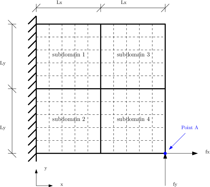
A bi-unit square of homogeneous elastic material is fixed at the left end and a constant force with components $f_{x}=f_{y}=1$ is applied at the right bottom corner. The Lamé parameters are taken as $\lambda=100$ and $\mu=100$ , and the mass density is taken as $\rho=100$ . The computational domain is decomposed into four equally sized square subdomains. Four node quadrilateral elements are used to form a 5-element by 5-element mesh for each subdomain. Figure 19 provides a pictorial description of the problem. A similar problem is also considered in Reference [22], which also addressed multi-time-step coupling method for structural dynamics.

The central difference scheme $(\beta=0,\gamma=1/2)$ is employed for subdomains 1, 2 and 3, and Newmark average acceleration scheme $(\beta=1/4,\gamma=1/2)$ is employed for subdomain 4. Figure 20 illustrates that the accuracy can be improved by decreasing the system time-step. Figure 21 illustrates that the accuracy need not always improve by decreasing subdomain time-steps for a fixed system time-step. This is completely in accordance with the theoretical predictions. The numerical results shown in Figure 21 also illustrate that the proposed coupling method allows subcycling in all the subdomains. This is evident from the fact that all the chosen values for $\eta_{i}\;(i=1,\cdots,S)$ are greater than unity. As it can be seen in Figure 22, subcycling can result in increase in drift. Figure 23 shows that there is no appreciable drift in displacements along the subdomain interface, and there is no drift in the velocities along the subdomain interface, as the proposed method imposes constraints on the continuity of velocities at every system time-step. Figure 24 shows that the theoretical bounds on the drifts in equations (115a)–(115b) match well with the numerical results. In all the numerical results, the proposed multi-time-step coupling method performed well, and behaved in accordance with the theoretical predictions derived in this paper.

9.4. Two-dimensional wave propagation problem

Consider the transverse motion of a plate subject governed by the following equations:


		$\displaystyle\frac{1}{c_{0}^{2}}\frac{\partial^{2}u}{\partial t^{2}}-\left(\frac{\partial^{2}u}{\partial x^{2}}+\frac{\partial^{2}u}{\partial y^{2}}\right)=f(\mathbf{x},t)\quad\forall\left(\mathbf{x},t\right)\in\Omega\times\mathcal{I}$		(152a)
		$\displaystyle u(\mathbf{x},t)=u^{\mathrm{p}}(\mathbf{x},t)\quad\left(\mathbf{x},t\right)\in\Gamma^{\mathrm{D}}\times\mathcal{I}$		(152b)
		$\displaystyle\mathrm{grad}[u]\cdot\widehat{\mathbf{n}}(\mathbf{x})=s^{\mathrm{p}}(\mathbf{x},t)\quad\left(\mathbf{x},t\right)\in\Gamma^{\mathrm{N}}\times\mathcal{I}$		(152c)
		$\displaystyle u(\mathbf{x},t=0)=u_{0}(\mathbf{x})\quad\mathbf{x}\in\Omega$		(152d)
		$\displaystyle\dot{u}(\mathbf{x},t=0)=v_{0}(\mathbf{x})\quad\mathbf{x}\in\Omega$		(152e)

where $u(\mathbf{x},t)$ is the transverse displacement, $c_{0}$ is the wave velocity, $f(\mathbf{x},t)$ is the forcing function, $\widehat{\mathbf{n}}(\mathbf{x})$ is the unit outward normal to the boundary, $u^{\mathrm{p}}(\mathbf{x},t)$ is the prescribed displacement on the boundary, $s^{\mathrm{p}}(\mathbf{x},t)$ is the prescribed transverse traction, and $u_{0}(\mathbf{x})$ and $v_{0}(\mathbf{x})$ are, respectively, the initial displacement and initial velocity. Computational domain is denoted by $\Omega$ . The part of the boundary on which Neumann boundary condition is denoted by $\Gamma^{\mathrm{N}}$ , and $\Gamma^{\mathrm{D}}$ is the part of the boundary on which Dirichlet boundary condition is prescribed. As usual, we assume that $\Gamma^{\mathrm{D}}\cap\Gamma^{\mathrm{N}}=\emptyset$ , and $\Gamma^{\mathrm{D}}\cup\Gamma^{\mathrm{N}}=\partial\Omega$ . The time interval of interest is $\mathcal{I}$ .

We consider the computational domain to be a rectangle with $L_{x}=2$ and $L_{y}=1$ . The boundary is fixed on three sides, and is excited by a sinusoidal force of the following form on the other side:

\displaystyle f(\mathbf{x},t)=\left\{\begin{array}[]{c}f_{0}\sin\left(\frac{2\pi}{\tau_{\mathrm{load}}}t\right)\quad t\in\left[0,\tau_{\mathrm{load}}\right]\\ 0\quad\quad\quad\quad\quad t>\tau_{\mathrm{load}}\end{array}\right.,\quad\mathbf{x}\in\{0\}\times[2L_{y}/5,3L_{y}/5]

A pictorial description of the problem is shown in Figure 25. The domain is decomposed into two subdomain, as shown in Figure 26. In this numerical example, we have taken $u_{0}=0$ , $v_{0}=0$ , $c_{0}=1$ , $f_{0}=5.0$ , and $\tau_{\mathrm{load}}=0.1$ . Figure 27 shows the result for explicit/implicit integration using the proposed coupling method. In this case, $(\gamma_{1},\beta_{1})=(1/2,0)$ , and $(\gamma_{2},\beta_{2})=(1/2,1/4)$ . The system time-step is $\Delta t=10^{-4}$ , subdomain time-steps are $\Delta t_{1}=10^{-5}$ and $\Delta t_{2}=10^{-4}$ . As one can see from this figure, the proposed coupling method performed well. In particular, there are no spurious reflections at the subdomain interface, and there is no noticeable drift in the transverse displacement along the subdomain interface.

This problem also clearly demonstrates that the proposed multi-time-step coupling method can be attractive for wave propagation problems. The coupling method is more cost effective than mere employing either an explicit scheme or an implicit scheme in the entire domain. In wave propagation problems involving fast dynamics, small time-steps are needed, and hence explicit schemes are typically employed. This will result in taking large number of time-steps to be able to carry out the numerical simulation to a desired final time. On the other hand, under the proposed coupling method, one can use explicit methods in the regions with fast dynamics (which typically occur near the loading), and use an implicit time-stepping scheme with a larger subdomain time-step in the other regions. For the chosen problem, if one has to employ an explicit scheme in the entire domain, the time-step should be smaller than the critical time-step of $1.36\times 10^{-5}$ . Under the proposed multi-time-step coupling method, the user can employ an explicit scheme with time-steps smaller than the critical time-step near the load, and an unconditionally stable, implicit time-stepping scheme with larger time-steps in the rest of the computational domain.

10. CONCLUDING REMARKS

We have developed a multi-time-step coupling method that can handle multiple subdomains with different time-steps in different subdomains. The coupling method can couple implicit and explicit time-stepping schemes under the Newmark family even with disparate time-steps of more than two orders of magnitude in different subdomains. A systematic study on the energy preservation and energy properties of the proposed coupling method is presented, and the corresponding sufficient conditions are also derived. The proposed coupling method, in general, is not energy preserving. Despite claims in the literature, the quest for energy preserving multi-time-step coupling method is still on. One of the main conclusions of this paper is about the effect of system time-step and subcycling on the accuracy. It has been shown that accuracy can always be improved by decreasing system time-step. It is widely believed that lowering subdomain time-step keeping the system time-step will also improve the accuracy under a multi-time-stepping scheme. Using careful mathematical analysis and numerical results, we have shown that this popular belief is not always the case. To this end, a simple criterion is also proposed, which can predict whether subcycling will improve accuracy. The criterion is to monitor $\mathcal{E}_{\mathrm{interface}}^{(n\rightarrow n+1)}$ at every system time-step, which can be calculated on the fly during a numerical simulation. Subcycling is desirable if this quantity is small.

The proposed multi-time-step coupling (which is a dual Schur domain decomposition technique) is well-suited for parallel computing. Specifically, one can utilize the advances made on the FETI method, which has shown to be scalable in a parallel setting for dual Schur domain decomposition methods [42]. There are several ways one could make advancements to the research presented in this paper. On the theoretical front, a plausible future work is to perform a mathematical analysis on the numerical characteristics of the proposed multi-time-step coupling method on the lines of local error, propagation of error, and influence of perturbations. On the computational implementation front, one could implement the proposed coupling method in a parallel setting and do a systematic study on its parallel performance. On the algorithmic front, the next logical step is to extend the proposed multi-time-step coupling method to first-order transient systems, and eventually to fluid-structure interaction problems.

11. APPENDIX: DERIVATION OF GOVERNING EQUATIONS FOR CONSTRAINED MULTIPLE SUBDOMAINS

One can derive the constrained governing equations for second-order transient systems in several ways. For example, in Reference [24] the equations have been derived using Lagrangian formalism. Herein, we shall derive the constrained governing equations for second-order systems using the Gauss principle of least constraint and Gibbs-Appell equations. Both these approaches can easily handle constraints of various types, including non-holonomic constraints and friction. Correctly, these two principles are considered more fundamental than Lagrangian or Hamiltonian formalisms, and are particularly ideal to deal with constraints [43]. We briefly outline these two powerful approaches with a hope that the future works on multi-time-step coupling methods will utilize either the Gauss principle of least constraint or the Gibbs-Appell equations.

11.1. Gauss principle of least constraint

The statement of Gauss principle of least constraint for a system of $N$ subdomains takes the following form:

		$\displaystyle\mathop{\mathrm{minimize}}_{\ddot{\boldsymbol{u}}_{1},\ddot{\boldsymbol{u}}_{2},\cdots,\ddot{\boldsymbol{u}}_{S}}\quad\frac{1}{2}\sum_{i=1}^{S}\left(\ddot{\boldsymbol{u}}_{i}-\boldsymbol{M}_{i}^{-1}\boldsymbol{h}_{i}\left(\dot{\boldsymbol{u}}_{i},\boldsymbol{u}_{i},t\right)\right)^{\mathrm{T}}\boldsymbol{M}_{i}\left(\ddot{\boldsymbol{u}}_{i}-\boldsymbol{M}_{i}^{-1}\boldsymbol{h}_{i}\left(\dot{\boldsymbol{u}}_{i},\boldsymbol{u_{i}},t\right)\right)$		(155)
		$\displaystyle\mbox{subject to}\quad\sum_{i=1}^{S}\boldsymbol{C}_{i}\ddot{\boldsymbol{u}}(t)=\boldsymbol{0}$		(156)

Note that in a continuum setting, continuity of displacements, velocities and accelerations are all equivalent. The first-order optimality condition gives rise to the following equations:


		$\displaystyle\boldsymbol{M}_{i}\ddot{\boldsymbol{u}}_{i}=\boldsymbol{h}_{i}(\dot{\boldsymbol{u}}_{i},\boldsymbol{u}_{i},t)+\boldsymbol{C}_{i}^{\mathrm{T}}\boldsymbol{\lambda}$		(157a)
		$\displaystyle\sum_{i=1}^{S}\boldsymbol{C}_{i}\ddot{\boldsymbol{u}}=\boldsymbol{0}$		(157b)

where $\boldsymbol{\lambda}$ is the vector of Lagrange multipliers for enforcing the constraint. Equations (157a)–(157b) are the governing equations for constrained multiple subdomains. In the case of linear elastic second-order systems, the vector $\boldsymbol{h}_{i}$ is given by the following expression:

\displaystyle\boldsymbol{h}_{i}(\dot{\boldsymbol{u}}_{i},\boldsymbol{u}_{i},t)=-\boldsymbol{K}_{i}\boldsymbol{u}_{i}+\boldsymbol{f}_{i}^{\mathrm{ext}}(t)

(158)

It is noteworthy that the question whether the vector $\boldsymbol{h}_{i}$ can depend on acceleration is still a matter of debate among mechanicians. For further details on this issue see [44, 45, 46, 47].

11.2. Gibbs-Appell equations

The statement of Gibbs-Appell principle for a system of $N$ subdomains can be written as follows:


		$\displaystyle\mathop{\mathrm{minimize}}_{\ddot{\boldsymbol{u}}_{1},\ddot{\boldsymbol{u}}_{2},\cdots,\ddot{\boldsymbol{u}}_{S}}\quad\sum_{i=1}^{S}\left(\frac{1}{2}{\ddot{\boldsymbol{u}_{i}}}^{\mathrm{T}}\boldsymbol{M}_{i}{\ddot{\boldsymbol{u}}}_{i}-{\ddot{\boldsymbol{u}}_{i}}^{\mathrm{T}}\boldsymbol{h}_{i}\right)$		(159a)
		$\displaystyle\mbox{subject to}\quad\sum_{i=1}^{S}\boldsymbol{C}_{i}\ddot{\boldsymbol{u}}_{i}=\boldsymbol{0}$		(159b)

The first-order optimality condition of the above constrained optimization problem gives rise to the same governing equations for constrained multiple subdomains (given by equations (157a)–(157b)).

ACKNOWLEDGMENTS

The authors acknowledge the support of the National Science Foundation under Grant no. CMMI 1068181. The opinions expressed in this paper are those of the authors and do not necessarily reflect that of the sponsor(s).

References

[1] J. T. Oden, T. Belytschko, J. Fish, T. J. R. Hughes, C. Johnson, D. Keyes, A. Laub, L. Petzold, D. Srolovitz, and S. Yip. Revolutionizing engineering science through simulation: A report of the national science foundation blue ribbon panel on simulation-based engineering science. National Science Foundation, Arlington, Virginia, 2006.
[2] A. Gravouil and A. Combescure. Multi-time-step explicit-implicit method for non-linear structural dynamics. International Journal for Numerical Methods in Engineering, 50:199–225, 2001.
[3] K. B. Nakshatrala, K. D. Hjelmstad, and D. A. Tortorelli. A FETI-based domain decomposition technique for time dependent first-order systems based on a DAE approach. International Journal for Numerical Methods in Engineering, 75:1385–1415, 2008.
[4] E. Hairer, S. P. Norsett, and G. Wanner. Solving Ordinary Differential Equations I: Nonstiff Problems. Springer-Verlag, New York, USA, second edition, 2011.
[5] T. Belytschko, H. J. Yen, and R. Mullen. Mixed methods for time integration. Computer Methods in Applied Mechanics and Engineering, 17–18:259–275, 1979.
[6] W. K. Liu and T. Belytschko. Mixed-time implicit-explicit finite elements for transient analysis. Computers and Structures, 15:445–450, 1982.
[7] T. Belytschko and R. Mullen. Explicit integration of structural problems. Finite Elements in Nonlinear Mechanics, 2:697–720, 1977.
[8] T. Belytschko and R. Mullen. Stability of explicit-implicit mesh partitions in time integration. International Journal of Numerical Methods in Engineering, 12:1575–1586, 1978.
[9] T. J. R. Hughes. Generalization of selective integration procedures to anisotropic and nonlinear media. International Journal for Numerical Methods in Engineering, 15:1413–1418, 1980.
[10] T. J. R. Hughes and W. K. Liu. Implicit-explicit finite elements in transient analysis: stability theory. Journal of Applied Mechanics, 45:371–374, 1978.
[11] T. J. R. Hughes and W. K. Liu. Implicit-explicit finite elements in non-linear transient analysis. Computer Methods in Applied Mechanics and Engineering, 17:159–182, 1979.
[12] P. Smolinski, T. Belytschko, and M. Neal. Multi-time-step integration using nodal partitioning. International Journal of Numerical Methods in Engineering, 26:349–359, 1988.
[13] W. J. T. Daniel. The subcycled Newmark algorithm. Computational Mechanics, 20:272–281, 1997.
[14] P. B. Nakshatrala, K. B. Nakshatrala, and D. A. Tortorelli. A time-staggered partitioned coupling algorithm for transient heat conduction. International Journal for Numerical Methods in Engineering, 78:1387–1406, 2009.
[15] A. Akkasale. Stability of Coupling Algorithms. Master’s thesis, Texas A&M University, College Station, Texas, USA, 2011. http://repository.tamu.edu/handle/1969.1/ETD-TAMU-2011-05-9500.
[16] L. Petzold. Differential/algebraic equations are not ODEs. SIAM Journal on Scientific and Statistical Computing, 3:367–384, 1982.
[17] K. B. Nakshatrala, A. Prakash, and K. D. Hjelmstad. On dual Schur domain decomposition method for linear first-order transient problems. Journal of Computational Physics, 228:7957–7985, 2009.
[18] U. M. Ascher and L. R. Petzold. Computer Methods for Ordinary Differential Equations and Differential-Algebraic Equations. SIAM, Philadelphia, USA, 1998.
[19] L. He G. Magonette A. Bonelli, O. S. Bursi and P. Pegon. Convergence Analysis of a Parallel Interfield Method for Heterogeneous Simulations with Dynamics Substructuring. International Journal For Numerical Methods in Engineering, 758:800–825, 2008.
[20] A. Bonelli O. S. Bursi, L. He and P. Pegon. Novel Generalized- $\alpha$ Methods for Interfield Parallel Integration of Heterogeneous Structural Dynamics Systems. Journal of Computational and Applied Mathematics, 234:2250–2258, 2010.
[21] A. Bonelli C. Jia, O. S. Bursi and Z. Wang. Novel Partitioned Time Integration Methods for DAE Systems Based on L-Stable Linearly Implicit Algorithms. International Journal for Numerical Methods in Engineering, 87:1148–1182, 2011.
[22] N. Mahjoubi and S. Krenk. Multi-time-step domain coupling method with energy control. International Journal for Numerical Methods in Engineering, 83:1700–1718, 2010.
[23] A. Combescure N. Mahjoubi, A. Gravouil and N. Greffet. A monolithic energy conserving method to couple heterogeneous time integrators with incompatible time steps in structural dynamics. Computer Methods in Applied Mechanics and Engineering, 200:1069–1086, 2011.
[24] A. Prakash and K. D. Hjelmstad. A FETI-based multi-time-step coupling method for Newmark schemes in structural dynamics. International Journal for Numerical Methods in Engineering, 61:2183–2204, 2004.
[25] T. J. R. Hughes. The Finite Element Method: Linear Static and Dynamic Finite Element Analysis. Prentice-Hall, Englewood Cliffs, New Jersey, USA, 1987.
[26] N. M. Newmark. A method of computation for structural dynamics. Journal of the Engineering Mechanics Division, ASCE, 85:67–94, 1959.
[27] W. L. Wood. Practical Time-Stepping Schemes. Oxford Univcersity Press, New York, USA, 1990.
[28] B. Leimkuhler and S. Reich. Simulating Hamiltonian Dynamics. Cambridge University Press, Cambridge, UK, 2005.
[29] M. Geradin and D. Rixen. Mechanical Vibrations: Theory and Applications to Structural Dynamics. John Wiley & Sons Ltd., Chichester, U.K., second edition, 1997.
[30] A. Toselli and O. Widlund. Domain Decomposition Methods. Springer-Verlag, New York, USA, 2004.
[31] C. W. Gear. Differential-algebraic equations, indices and integral algebraic equations. SIAM Journal on Numerical Analysis, 27:1527–1534, 1990.
[32] K. Brenan, S. Campbell, and L. Petzold. Numerical Solutions of Initial-Value Problems in Differential-Algebraic Equations. North-Holland, New York, USA, 1989.
[33] M. Geradin and A. Cardona. Flexible Multibody Dynamics: A Finite Element Approach. John Wiley & Sons Ltd., Chichester, U.K., 2001.
[34] J. Baumgarte. Stabilization of constraints and integrals of motion in dynamical systems. Computer Methods in Applied Mechanics and Engineering, 1:1–16, 1972.
[35] A. Younes, P. Ackerer, and F. Lehmann. Stability and accuracy analysis of Baumgarte’s constraint violation stabilization method. ASME Journal of Mechanical Design, 117:446–453, 1995.
[36] O. A. Bauchau. Review of contemporary approaches for constraint enforcement in multibody systems. Journal of Computational and Nonlinear Dynamics, 3:1–8, 2008.
[37] P. Flores, R. Pereira, M. Machado, and E. Seabra. Investigation on the Baumgarte stabilization method for dynamic analysis of constrained multibody systems. Proceedings of EUCOMES 08, pages 305–312, 2009.
[38] A. Prakash. Multi-time-step Domain Decomposition and Coupling Methods for Non-linear Structural Dynamics. PhD thesis, University of Illinois at Urbana-Champaign, Urbana, Illinois, USA, 2007.
[39] L. C. Evans. Partial Differential Equations. American Mathematical Society, Providence, Rhode Island, USA, 1998.
[40] R. D. Richtmyer and K. W. Morton. Difference Methods for Initial-Value Problems. Krieger Publishing Company, Malabar, Florida, USA, 1994.
[41] E. Hairer and G. Wanner. Solving Ordinary Differential Equations II: Stiff and Differential-Algebraic Problems. Springer-Verlag, New York, USA, 1996.
[42] C. Farhat and F. Roux. A method of finite element tearing and interconnecting and its parallel solution algorithm. International Journal for Numerical Methods in Engineering, 32:1205–1227, 1991.
[43] F. E. Udwadia and R. E. Kalaba. Analytical Dynamics: A New Approach. Cambridge University Press, Cambridge, UK, 2007.
[44] L. A. Pars. Introduction to Dynamics. Cambridge University Press, Cambridge, UK, 1953.
[45] YH Chen. Pars’s acceleration paradox. Journal of the Franklin Institute, 335(5):871–875, 1998.
[46] C. M. Leech. The given force cannot be a function of acceleration. Technische Mechanik, 16:221–226, 1996.
[47] M.M. Zhechev. On the admissibility of given acceleration-dependent forces in mechanics. Journal of applied mechanics, 74(1):107–110, 2007.

Refer to caption — Figure 1. A pictorial description of multiple subdomains. The domain $\Omega$ is decomposed into $S$ subdomains, which are denoted by $\Omega_{1},\cdots,\Omega_{S}$ . The subdomain interface is indicated using dashed curves. The mesh is assumed to be conforming along the subdomain interface.