Degree Distribution in Quantum Walks on Complex Networks

In the classical walk the probability $P_{i}(t)$ of being at node $i$ at time $t$ evolves as $|P(t)\rangle=S(t)|P(0)\rangle$, where $|P(t)\rangle=\sum_{i}P_{i}(t)|i\rangle$. The stationary states of the walk are described by eigenvectors $|\pi_{i}^{k}\rangle$ of $H_{C}$ with eigenvalues $\lambda_{i}$ equal to zero. We assume throughout this work that the walk is connected, i.e., it is possible to transition from any node to any other node through some series of allowed transitions. In this case there is a unique eigenvector $|\pi_{0}\rangle=|P_{C}\rangle$ with $\lambda_{0}=0$, and $\lambda_{i}>0$ for all $i\neq 0$ [44, 45, 46, 41]. This (normalized) eigenvector $|P_{C}\rangle=\sum_{i}(P_{C})_{i}|i\rangle$ describes the steady state distribution

In other words, the process is ergodic and after long times the probability of finding the walker at any node $i$ is given purely by the importance of the degree $d_{i}$ of that node in the network underlying the process.

When considering quantum walks on networks, it is natural to ask what is the long time behavior of a quantum walker [11, 15, 47, 22]. The unitary evolution will not drive the system towards a steady state. Therefore, to obtain a static picture we consider the long time average probability $(P_{Q})_{i}$ of being on node $i$, which reads

For ease of comparison with $|P_{C}\rangle$ we will also write the distribution in Eq. (3) as a ket $|P_{Q}\rangle=\sum_{i}(P_{Q})_{i}|i\rangle$. Unlike the classical case, Eq. (2) depends on the initial state $\rho(0)$.

Interference between subspaces of different energy vanish in the long time average so we obtain an expression for the probability $(P_{Q})_{i}$ in terms of the energy eigenspace projectors $\Pi_{j}$ of the Hamiltonian $H_{Q}$,

Here $\Pi_{j}=\sum_{k}|\phi_{j}^{k}\rangle\langle\phi_{j}^{k}|$ projects onto the subspace spanned by the eigenvalues $|\phi_{j}^{k}\rangle$ of $H_{Q}$ corresponding to the same eigenvalue $\lambda_{j}$. In other words, the long time average distribution is a mixture of the distributions obtained by projecting the initial state onto each eigenspace.

Due to the similarity transformation $H_{Q}=D^{-\nicefrac{{1}}{{2}}}H_{C}D^{\nicefrac{{1}}{{2}}}$ the classical $H_{C}$ and quantum $H_{Q}$ generators share the same eigenvalues $\lambda_{i}\geq 0$, and have eigenvectors related by $|\phi_{i}^{k}\rangle=D^{-\nicefrac{{1}}{{2}}}|\pi_{i}^{k}\rangle$ up to their normalizations. In particular, the unique eigenvectors corresponding to $\lambda_{0}=0$ are $|\pi_{0}\rangle=D|\mathbf{1}\rangle$ and $|\phi_{0}\rangle=D^{\nicefrac{{1}}{{2}}}|\mathbf{1}\rangle$ up to their normalizations, with $|\mathbf{1}\rangle=\sum_{i}|i\rangle$. Therefore the probability vector describing the outcomes of a measurement of the quantum ground state eigenvector $|\phi_{0}\rangle$ in the node basis is the classical steady state distribution $|\pi_{0}\rangle=|P_{C}\rangle$.

The state vector $|P_{C}\rangle$ appears in Eq. (3) for the quantum long time average distribution $|P_{Q}\rangle$ with weight $\langle\phi_{0}|\rho(0)|\phi_{0}\rangle$. Accordingly we split the sum in Eq. (3) into two parts, the first we call the “classical term” $|P_{C}\rangle$ and the rest we call the “quantum correction” $|\tilde{P}_{Q}\rangle$, as

The normalized quantum correction $|\tilde{P}_{Q}\rangle=\sum_{i}(\tilde{P}_{Q})_{i}|i\rangle$ is given by

and the weight

we call quantumness is a function both of the degrees, through $|\phi_{0}\rangle$, and the initial state.

We can think of the parameter $\varepsilon$, which controls the classical-quantum mixture, as the quantumness of $|P_{Q}\rangle$ for the following three reasons. First, the proportion of the elements in $(P_{Q})_{i}$ that corresponds to the quantum correction is $\varepsilon$. Second, the trace distance between the normalized distribution $(P_{C})_{i}$ and the unnormalized distribution $(1-\varepsilon)(P_{C})_{i}$ forming the classical part of the quantum result is also $\varepsilon$. Last, using a triangle inequality, the trace distance between the normalized distributions $(P_{C})_{i}$ and $(P_{Q})_{i}$ is upper bounded by $2\varepsilon$.

This expression for the quantumness in Eq. (6) enables us to make some physical statements about a general initial state. By realizing that $|\phi_{0}\rangle$ is the ground state of zero energy $\lambda_{0}=0$ and the gap $\Delta=\min_{i\neq 0}\lambda_{i}$ in the energy spectrum is non-zero for a connected network [44, 45, 46, 41], the above implies a bound $E/\Delta\geq\varepsilon$ for the quantumness $\varepsilon$ of the walk in terms of the energy $E=\textrm{tr}\{H_{Q}\rho\}$ of the initial state. The bound is obtained through the following steps

The above demonstrates that the classical stationary probability distribution will be recovered for low energies. A utility of this result is that it connects the long time average distribution to a simple physical property of the walk, the energy, which provides a total ordering of all possible initial states.

Quantumness is both a function of the degrees of the network nodes and the initial state. To compare the quantumness of different complex networks, we fix the initial state $\rho(0)$. For our example we choose the even superposition state $\rho(0)=|\Psi(0)\rangle\langle\Psi(0)|$ with $|\Psi(0)\rangle=|\mathbf{1}\rangle/\sqrt{N}$. This state has several appealing properties, for example, it is invariant under node permutations and independent of the arrangement of the network.

In this case the quantumness is given by the expression

where $\langle d\rangle=\sum_{i}d_{i}/N$ is the average degree and $\langle\sqrt{d}\rangle=\sum_{i}\sqrt{d}_{i}/N$ is the average root degree of the nodes. As such, the quantumness depends only on the degree distribution of the network and increases with network heterogeneity.

This statement is quantified by writing the quantumness

in terms of the Rényi entropy

where $d_{i}/\sum_{j}d_{j}=(P_{C})_{i}$ are the normalized degrees.

To obtain an expression in terms of the (perhaps) more familiar Shannon entropy $H_{1}$ (obtained by taking the $q\rightarrow 1$ limit of Eq. (10)), we recall that the Rényi entropy is non-increasing with $q$ [48]. This leads to the upper bound

The quantumness approaches this upper bound in the limit that $M$ nodes have uniform degree $d_{i}=M\langle d\rangle/N$ and all others have $d_{i}=0$. This limit is never achieved unless $M=N$ and $\varepsilon=0$, e.g., a regular network. Physically, $\varepsilon=0$ for a regular network because the symmetry of the Hamiltonian $H_{Q}$ implies its eigenvectors are evenly distributed. The only eigenvector of this type that is positive is the initial state $|\Psi(0)\rangle$, which due to the Perron-Frobenius theorem must also be the ground state $|\Psi(0)\rangle=|\phi_{0}\rangle$. Therefore $E=0$ and so, from Eq. (7), $\varepsilon=0$.

In another limit, the quantumness takes its maximum value $\varepsilon=(N-2)/N\approx 1$ when the degrees of two nodes are equal and much larger than those of the others (note that the symmetry of $A$ prevents the degree of a single node from dominating). In the case that $A_{ij}\in\{0,1\}$, i.e., the network underlying the walks is not weighted, the quantumness of a connected network is more restricted. It is maximized by a walk based on a star network—where a single node is connected to all others. For a walk of this type $\varepsilon=1/2-\sqrt{N-1}/N\approx 1/2$.

Next, in Sec. III we confirm the above analytical findings numerically and at the same time numerically study the form of the quantum correction $|\tilde{P}_{Q}\rangle$ given by Eq. (5) for a range of complex network topologies.

We consider walkers on model networks, each with a fundamentally different complex network topology. To start, we consider non-weighted binary networks $A_{ij}\in\{0,1\}$ with $N=500$ nodes and average degree $\langle d\rangle\approx 6$. If a disconnected network is obtained, only the giant component is considered. Specifically we consider the ba scale free network [25], the er [49] and the ws [50] small world networks, and the rg (on a square) [51], a network without the scale free or small world characteristics.

The long time average probability of being on each node $i$ is plotted against its degree $d_{i}$ for a quantum ($P_{Q}$) and stochastic ($P_{C}$) walk in Fig. 2. The two cases are nearly identical for these binary networks and the evenly distributed initial state, illustrating that the quantumness $\varepsilon$ is small. We have in fact calculated the quantumness directly for each network type, yielding $\varepsilon=0.130,0.043,0.016,0.040$ for the ba, er, ws and rg networks, respectively. Within these, the ba network shows the highest quantum correction. This is expected since the ba network has the higher degree heterogeneity. The ws network, which is well known to have quite uniform degrees [52], is accordingly the network with the lowest quantum correction.

For many of the network types the typical quantumness can be obtained from the expected (thermodynamic limit) degree distribution. In the ba network, the degree distribution approximately obeys the continuous probability density $P(d)=\langle d\rangle^{2}/2d^{3}$ [25]. Integrating this to find the moments, results in $\varepsilon=1/9$, which is independent of the average degree $\langle d\rangle$ and is compatible with our numerics. The degree distributions of the er and rg networks both approximately follow the Poissonian distribution $P(d)\approx\langle d\rangle^{d}\mathrm{e}^{-\langle d\rangle}/d!$ for large networks, which explains the similarity of their quantumness $\varepsilon$ values. For $\langle d\rangle=6$ we recover $\varepsilon\approx 0.046$, which is compatible with the values for the particular networks we generated. From the general form, calculating the quantumness numerically and performing a best fit we find that $\varepsilon\approx\kappa_{1}\langle d\rangle^{-\kappa_{2}}$, with fitting parameters $\kappa_{1}=0.429$ and $\kappa_{2}=1.210$.

The size of the quantum effects can be enhanced by introducing heterogeneous weights $A_{ij}$ within a network. We have done this for a ba network using several iterations of the following procedure. A pair of connected nodes is randomly selected then the associated weight is doubled of halved at random. As anticipated, the effect is to increase the discrepancy between the classical and quantum dependence of the long time average probability on degree, illustrated in Fig. 2. As the number of iterations is increased, the quantumness follows the bound given in Eq. (11), as shown in Fig. 3. In fact, most networks are found close to saturating this bound, especially for low quantumness.

Further, the energy $E=\langle\Psi_{0}|H_{Q}|\Psi_{0}\rangle$ of the given initial state has a simple expression $E=1-(1/N)\sum_{ij}A_{ij}/\sqrt{d_{i}d_{j}}$, which allows us to determine the extent to which the bound $E/\Delta\geq\varepsilon$ is saturated by comparing the values of $E/\Delta$ and $\varepsilon$. We find that for some networks, e.g., the BA, ER and WS networks, the bound is quite restrictive and reasonably saturated. However for the other networks we find that quantumness takes a low value without this being ensured by the bound only, see Table 1.

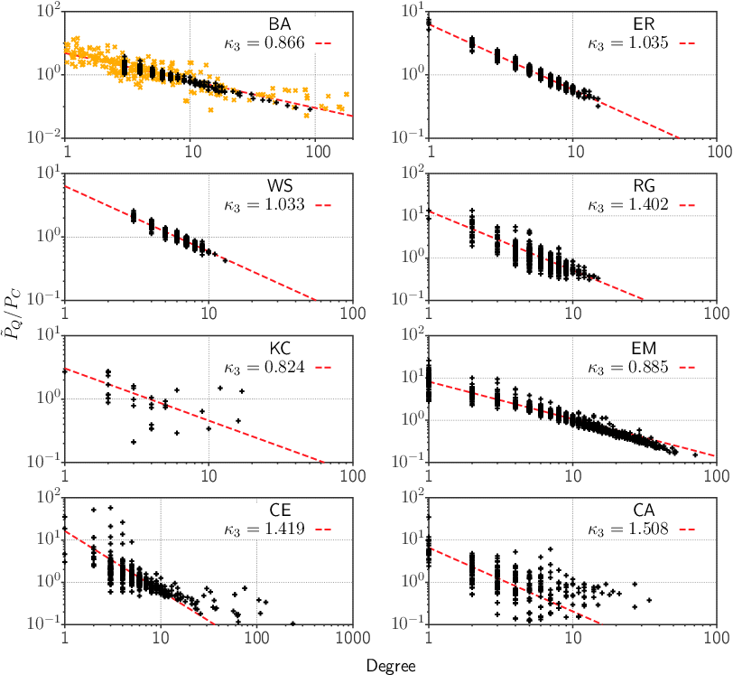
Finally, our numerical calculations reveal the behavior of the quantum part $\tilde{P}_{Q}$ of the long time average node occupation. We find that the quantum part enhances the long time average probability of being at nodes with small degree relative to the classical part. More precisely $(\tilde{P}_{Q})_{i}/(P_{C})_{i}$ exhibits roughly $(d_{i})^{-\kappa_{3}}$ scaling, with $\kappa_{3}\approx 1$, as shown in Fig. 4. Interestingly, there is a correlation between the amount of enhancement, given by $\kappa_{3}$, and the type of complex network. The network types with smaller diameters (order of increasing diameter: ba, then er and ws, then rg) have the smallest $\kappa_{3}$, and the quantum parts enhance the low degree nodes least. Moreover, the enhancement $\kappa_{3}$ seems to be quite independent of the internode weights. Thus our numerics show a qualitatively common quantum effect for a range of complex network types. Quantitative details vary between the network types, but appear robust within each type.

The models of networks examined in the previous subsection have very specific topologies and therefore degree distributions, and do not capture the topological properties of all real-world networks (for details see chapter 9 of Ref. [30]). We therefore now study the behavior of the quantumness and gap for topologies present in a variety of real-world networks: a kc (kc) social network [37], the em (em) network of the URV university [38], the ce (ce) network [39], and a ca (ca) network of scientists [40].

The values of the quantumness and comparison against the entropic upper bound are shown in Fig. 3. Despite the variety of topologies, we again find that the quantumness is consistently small. Therefore the classical and quantum distributions are very close, as shown in Fig. 2. Additionally, the quantum correction exhibits the same generic behavior as observed for the artificial networks; figure 4 shows an enhancement of the probability of being in nodes of small degree. Interestingly, the quantumness of real-world networks is appreciably smaller than enforced by the bound of Eq. (7), with $E/\varepsilon\Delta$ taking large values, as shown in Table 1.

References

- [1] Martí Cuquet and John Calsamiglia, “Entanglement percolation in quantum complex networks,” Phys. Rev. Lett. 103, 240503 (2009).
- [2] S Perseguers, M Lewenstein, A Acín, and JI Cirac, “Quantum random networks,” Nature Physics 6, 539–543 (2010a).
- [3] S. Perseguers, D. Cavalcanti, G. J. Lapeyre, M. Lewenstein, and A. Acín, “Multipartite entanglement percolation,” Phys. Rev. A 81, 032327 (2010b).
- [4] Richard P. Feynman, Robert B. Leighton, and Matthew Sands, The Feynman Lectures on Physics, 2nd ed. (Addison Wesley, 2005).
- [5] Richard P. Feynman and A.R. Hibbs, Quantum Mechanics and Path Integrals, International series in pure and applied physics (McGraw-Hill, 1965).
- [6] Andrew M. Childs, “Universal computation by quantum walk,” Phys. Rev. Lett. 102, 180501 (2009).
- [7] E. Farhi and S. Gutmann, “Quantum computation and decison trees,” Phys. Rev. A 58, 915–928 (1998).
- [8] F. Caruso, A. W. Chin, A. Datta, S. F. Huelga, and M. B. Plenio, “Highly efficient energy excitation transfer in light-harvesting complexes: The fundamental role of noise-assisted transport,” The Journal of Chemical Physics 131, 105106 (2009).
- [9] M. Mohseni, P. Rebentrost, S. Lloyd, and A. Aspuru-Guzik, “Environment-assisted quantum walks in photosynthetic energy transfer,” J. Chem. Phys. 129, 174106 (2008).
- [10] Yuan-Chung Cheng and Graham R. Fleming, “Dynamics of light harvesting in photosynthesis,” Annual Review of Physical Chemistry 60, 241–262 (2009), pMID: 18999996 .
- [11] E. Sánchez-Burillo, J. Duch, J. Gómez-Gardeñes, and D. Zueco, “Quantum Navigation and Ranking in Complex Networks,” Nat. Sci. Rep. 2, 605 (2012), 10.1038/srep00605.
- [12] G. D. Paparo and M. A. Martin-Delgado, “Google in a quantum network,” Sci. Rep. 2, 444 (2012).
- [13] Silvano Garnerone, Paolo Zanardi, and Daniel A. Lidar, “Adiabatic quantum algorithm for search engine ranking,” Phys. Rev. Lett. 108, 230506 (2012).
- [14] Silvano Garnerone, “Thermodynamic formalism for dissipative quantum walks,” Phys. Rev. A 86, 032342 (2012).
- [15] O. Mülken and A. Blumen, “Continuous-time quantum walks: Models for coherent transport on complex networks,” Phys. Rep. 502, 37–87 (2011).
- [16] Oliver Muelken, “Inefficient quantum walks on networks: the role of the density of states,” arXiv preprint arXiv:0710.3453 (2007).
- [17] Oliver Mülken, Veronika Bierbaum, and Alexander Blumen, “Coherent exciton transport in dendrimers and continuous-time quantum walks,” The Journal of chemical physics 124, 124905 (2006).
- [18] Chengzhen Cai and Zheng Yu Chen, “Rouse dynamics of a dendrimer model in the condition,” Macromolecules 30, 5104–5117 (1997).
- [19] S Salimi, “Continuous-time quantum walks on semi-regular spidernet graphs via quantum probability theory,” Quantum Information Processing 9, 75–91 (2010).
- [20] Herbert Spohn, “An algebraic condition for the approach to equilibrium of an open n-level system,” Letters in Mathematical Physics 2, 33–38 (1977).
- [21] James D. Whitfield, César A. Rodríguez-Rosario, and Alán Aspuru-Guzik, “Quantum stochastic walks: A generalization of classical random walks and quantum walks,” Physical Review A 81, 022323 (2010), arXiv:0905.2942 .
- [22] Oliver Mülken, Antonio Volta, and Alexander Blumen, “Asymmetries in symmetric quantum walks on two-dimensional networks,” Physical Review A 72, 042334 (2005).
- [23] Michalis Faloutsos, Petros Faloutsos, and Christos Faloutsos, “On power-law relationships of the internet topology,” SIGCOMM Comput. Commun. Rev. 29, 251–262 (1999).
- [24] R. Albert, H. Jeong, and A.L. Barabási, “Internet: Diameter of the world-wide web,” Nature 401, 130–131 (1999).
- [25] A.-L. Barabási and R. Albert, “Emergence of scaling in random networks,” Science 286, 509–512 (1999).
- [26] Réka Albert and Albert-László Barabási, “Statistical mechanics of complex networks,” Rev. Mod. Phys. 74, 47–97 (2002).
- [27] M. E. J. Newman, “The structure and function of complex networks,” SIAM Review 45, 167–256 (2003).
- [28] Mark Newman, Networks: An Introduction (Oxford University Press, Inc., New York, NY, USA, 2010).
- [29] D. J. de Solla Price, “Networks of scientific papers,” Science 149, 510–515 (1965).
- [30] Ernesto Estrada, The Structure of Complex Networks: Theory and Applications (Oxford University Press, 2011).
- [31] Stanley Wasserman and Katherine Faust, Social Network Analysis. Methods and Applications (Cambridge University Press, 1994).
- [32] Duncan J. Watts, Peter Sheridan Dodds, and M. E. J. Newman, “Identity and search in social networks,” Science 296, 1302–1305 (2002).
- [33] M. E. J. Newman, “Spread of epidemic disease on networks,” Phys. Rev. E 66, 016128 (2002).
- [34] Zoltan Zimboras, Mauro Faccin, Zoltan Kadar, James Whitfield, Ben Lanyon, and Jacob Biamonte, “Quantum transport enhancement by time-reversal symmetry breaking,” Sci. Rep. 3 (2013), 10.1038/srep02361.
- [35] J. Kempe, “Quantum random walks: an introductory overview,” Contemp. Phys. 44, 307–327 (2003).
- [36] Salvador Elias Venegas-Andraca, “Quantum walks for computer scientists,” Synthesis Lectures on Quantum Computing 1, 1–119 (2008).
- [37] Wayne W Zachary, “An information flow model for conflict and fission in small groups,” Journal of anthropological research , 452–473 (1977).
- [38] Roger Guimera, Leon Danon, A Diaz-Guilera, Francesc Giralt, and Alex Arenas, “Self-similar community structure in a network of human interactions,” Physical review E 68, 065103 (2003).
- [39] Jordi Duch and Alex Arenas, “Community detection in complex networks using extremal optimization,” Physical review E 72, 027104 (2005).
- [40] Mark E.J. Newman, “Finding community structure in networks using the eigenvectors of matrices,” Physical review E 74, 036104 (2006).
- [41] John C. Baez and Jacob Biamonte, “A course on quantum techniques for stochastic mechanics,” (2012), 235 pages, arXiv:1209.3632 .
- [42] T. H. Johnson, S. R. Clark, and D. Jaksch, “Dynamical simulations of classical stochastic systems using matrix product states,” Phys. Rev. E 82, 036702 (2010).
- [43] J. C. Baez and B. Fong, “A Noether theorem for Markov processes,” Journal of Mathematical Physics 54, 013301 (2013), arXiv:1203.2035 [math-ph] .
- [44] Joel Keizer, “On the solutions and the steady states of a master equation,” Journal of Statistical Physics 6, 67–72 (1972).
- [45] Peter Lancaster and Miron Tismenetsky, Theory of matrices, Vol. 2 (Academic Press New York, 1985).
- [46] James R Norris, Markov chains, 2008 (Cambridge University Press, 1998).
- [47] Dorit Aharonov, Andris Ambainis, Julia Kempe, and Umesh Vazirani, “Quantum walks on graphs,” in Proceedings of the thirty-third annual ACM symposium on Theory of computing (ACM, 2001) pp. 50–59.
- [48] C Beck and F Schögl, Thermodynamics of chaotic systems: an introduction (Cambridge University Press, 1993).
- [49] P. Erdős and A. Rényi, “On the Evolution of Random Graphs,” in Publication of the Mathematical Institute of the Hungarian Academy of Sciences (1960) pp. 17–61.
- [50] D. J. Watts and S. H. Strogatz, “Collective dynamics of ‘small-world’ networks,” Nature 393, 409–410 (1998).
- [51] Mathew Penrose, Random Geometric Graphs, Vol. 5 (Oxford University Press on Demand, 2003).
- [52] Alain Barrat and M. Weigt, “On the properties of small-world network models,” The European Physical Journal B 13, 547–560 (2000).
V Acknowledgments
We thank Michele Allegra, Ville Bergholm, Stephen Kirkland, Giovanni Petri and Simone Severini for fruitful discussions. JDB would like to thank the Qatar Environment and Energy Research Institute (QEERI) where part of this research was completed. PM would like to acknowledge the Spanish MINCIN/MINECO project TOQATA (FIS2008-00784), EU Integrated Projects AQUTE and SIQS, and HISTERA project DIQUIP.