DESY 13–079 ISSN 0418-9833
May 2013
Average gluon and quark jet multiplicities at higher orders
Abstract
We develop a new formalism for computing and including both the perturbative and nonperturbative QCD contributions to the scale evolution of average gluon and quark jet multiplicities. The new method is motivated by recent progress in timelike small- resummation obtained in the factorization scheme. We obtain next-to-next-to-leading-logarithmic (NNLL) resummed expressions, which represent generalizations of previous analytic results. Our expressions depend on two nonperturbative parameters with clear and simple physical interpretations. A global fit of these two quantities to all available experimental data sets that are compatible with regard to the jet algorithms demonstrates by its goodness how our results solve a longstandig problem of QCD. We show that the statistical and theoretical uncertainties both do not exceed 5% for scales above 10 GeV. We finally propose to use the jet multiplicity data as a new way to extract the strong-coupling constant. Including all the available theoretical input within our approach, we obtain in the scheme in an approximation equivalent to next-to-next-to-leading order enhanced by the resummations of terms through the NNLL level and of terms by the renormalization group, in excellent agreement with the present world average.
PACS numbers: 12.38.Cy, 12.39.St, 13.66.Bc, 13.87.Fh
1 Introduction
The production of hadrons is due to the strong interactions of quarks and gluons. Quantum chromodynamics (QCD), the gauge theory of the strong interactions, provides a quantitative description of the transitions from quarks and gluons to jets of hadrons, which may be tested experimentally. When jets are produced at colliders, they can be initiated either by a quark or a gluon. The two types of jets are expected to exhibit different properties, above all because quarks and gluons carry different color charges and spin. In fact, a gluon jet is typically broader and contains a larger amount of hadrons. Jets with different mother partons can also be studied by looking for the jet charge distribution as discussed in Ref. [1], with important consequences for the physics at the CERN Large Hadron Collider (LHC). To understand the interplay of quarks and gluons in a jet and to predict testable consequences thereof lies at the very core of QCD.
The typical way to depict the production of a jet from a parton (quark or gluon) is the following. An initial parton starts radiating gluons, which in turn can radiate further gluons or split into secondary quark-antiquark pairs. This so-called parton showering process causes the virtualities of the parent partons to decrease. Finally, when the virtuality falls below a certain cutoff, the cascade stops and the final-state partons hadronize into color-neutral hadrons, a process usually described by phenomenological models. This happens because the production of hadrons is a typical process where nonperturbative phenomena are involved. However, for particular observables, this problem can be avoided. In particular, the counting of hadrons in a jet that is initiated at a certain scale belongs to this class of observables. In this case, one can adopt with quite high accuracy the hypothesis of Local Parton-Hadron Duality (LPHD), which simply states that parton distributions are renormalized in the hadronization process without changing their shapes [2]. Hence, if the scale is large enough, this would in principle allow perturbative QCD to be predictive without the need to consider phenomenological models of hadronization. Nevertheless, such processes are dominated by soft-gluon emissions, and it is a well-known fact that, in such kinematic regions of phase space, fixed-order perturbation theory fails, rendering the usage of resummation techniques indispensable. As we shall see, the computation of avarage jet multiplicities indeed requires small- resummation, as was already realized a long time ago [3]. In Ref. [3], it was shown that the singularities for , which are encoded in large logarithms of the kind , spoil perturbation theory, and also render integral observables in ill-defined, disappear after resummation. Usually, resummation includes the singularities from all orders according to a certain logarithmic accuracy, for which it restores perturbation theory.
Small- resummation has recently been carried out for timelike splitting fuctions in the factorization scheme, which is generally preferable to other schemes, yielding fully analytic expressions. In a first step, the next-to-leading-logarithmic (NLL) level of accuracy has been reached [4, 5]. In a second step, this has been pushed to the next-to-next-to-leading-logarithmic (NNLL), and partially even to the next-to-next-to-next-to-leading-logarithmic (N3LL), level [6]. Thanks to these results, we are able to analytically compute the NNLL contributions to the evolutions of the average gluon and quark jet multiplicities with normalization factors evaluated to next-to-leading (NLO) and approximately to next-to-next-to-next-to-order (N3LO) in the expansion. The previous literature contains a NLL result on the small- resummation of timelike splitting fuctions obtained in a massive-gluon scheme. Unfortunately, this is unsuitable for the combination with available fixed-order corrections, which are routinely evaluated in the scheme. A general discussion of the scheme choice and dependence in this context may be found in Refs. [7, 8].
The average gluon and quark jet multiplicities, which we denote as and , respectively, represent the avarage numbers of hadrons in a jet initiated by a gluon or a quark at scale . In the past, analytic predictions were obtained by solving the equations for the generating functionals in the modified leading-logarithmic approximation (MLLA) in Ref. [9] through N3LO in the expansion parameter , i.e. through . However, the theoretical prediction for the ratio given in Ref. [9] is about 10% higher than the experimental data at the scale of the boson, and the difference with the data becomes even larger at lower scales, although the perturbative series seems to converge very well. An alternative approach was proposed in Ref. [10], where a differential equation for the average gluon-to-quark jet multiplicity ratio was obtained in the MLLA within the framework of the colour-dipole model, and the constant of integration, which is supposed to encode nonperturbative contributions, was fitted to experimental data. A constant offset to the average gluon and quark jet multiplicities was also introduced in Ref. [11].
Recently, we proposed a new formalism [12, 13] that solves the problem of the apparent good convergence of the perturbative series and does not require any ad-hoc offset, once the effects due to the mixing between quarks and gluons are fully included. Our result is a generalization of the result obtained in Ref. [9]. In our new approach, the nonperturbative informations to the gluon-to-quark jet multiplicity ratio are encoded in the initial conditions of the evolution equations. Motivated by the excellent agreement of our results with the experimental data found in Ref. [13], we propose here to also use our approach to extract the strong-coupling constant at some reference scale and thus extend our analysis by adding an apropriate fit parameter.
The paper is organized as follows. In Section 2, we introduce the equations governing the evolution of the average gluon and quark jet multiplicities with the scale at which the jet is initiated, develop a formalism to solve them, and improve our results by resummation. In Section 3, we explain how we can predict the average-jet-multiplicity evolutions in our framework adding as much as possible available information on small- timelike resummation. In Section 4, we fit our resummed formulae to the available experimental data exctracting the initial conditions for the evolutions, and discuss the uncertainties coming from both the statistical analysis of the data and the missing higher-order terms. In Section 5, we inject the strong-coupling constant into our analysis and extract it. Finally, in Section 6, we summarize our conclusions and present an outlook.
2 Fragmentation functions and their evolution
When one considers average multiplicity observables, the basic equation is the one governing the evolution of the fragmentation functions for the gluon–quark-singlet system . In Mellin space, it reads:
| (1) |
where , with , are the timelike splitting functions, , with being the standard Mellin moments with respect to , and is the couplant. The standard definition of the hadron multiplicities in terms of the fragmentation functions is given by their integral over , which clearly corresponds to the first Mellin moment, with (see, e.g., Ref. [14]):
| (2) |
where for a gluon and quark jet, respectively.
The timelike splitting functions in Eq. (1) may be computed perturbatively in ,
| (3) |
The functions for in the scheme may be found in Refs. [15, 16, 17] through NNLO and in Refs. [4, 5, 6] with small- resummation through NNLL accuracy. In the remainder of this section, we explain in detail our new approach to solve Eq. (1) in order to use its solution in Eq. (2) to obtain the average gluon and quark jet multiplicities. To this end, we first discuss how Eq. (1) can be diagonalized and then how to implement resummation to improve it, so as to obtain well-defined quantities at .
2.1 Diagonalization
It is not in general possible to diagonalize Eq. (1) because the contributions to the timelike-splitting-function matrix do not commute at different orders. The usual approach is then to write a series expansion about the leading-order (LO) solution, which can in turn be diagonalized. One thus starts by choosing a basis in which the timelike-splitting-function matrix is diagonal at LO (see, e.g., Ref. [18]),
| (4) |
with eigenvalues . In one important simplification of QCD, namely super Yang-Mills theory, this basis is actually more natural than the basis because the diagonal splitting functions may there be expressed in all orders of perturbation theory as one universal function with shifted arguments [19].
It is convenient to represent the change of basis for the fragmentation functions order by order for as [18]:
| (5) |
This implies for the components of the timelike-splitting-function matrix that
| (6) |
where
| (7) |
Our approach to solve Eq. (1) differs from the usual one in that we write the solution expanding about the diagonal part of the all-order timelike-splitting-function matrix in the plus-minus basis, instead of its LO contribution. For this purpose, we rewrite Eq. (4) in the following way:
| (8) |
In general, the solution to Eq. (1) in the plus-minus basis can be formally written as
| (9) |
where denotes the path ordering with respect to and
| (10) |
As anticipated, we make the following ansatz to expand about the diagonal part of the timelike-splitting-function matrix in the plus-minus basis:
| (11) |
where
| (12) |
is the diagonal part of Eq. (8) and is a matrix in the plus-minus basis which has a perturbative expansion of the form
| (13) |
In the following, we make use of the renormalization group (RG) equation for the running of ,
| (14) |
where
| (15) |
with , , and being colour factors and being the number of active quark flavours. Using Eq. (14) to perform a change of integration variable in Eq. (11), we obtain
| (16) |
Substituting then Eq. (13) into Eq. (16), differentiating it with respect to , and keeping only the first term in the expansion, we obtain the following condition for the matrix:
| (17) |
where
| (18) |
Solving it, we find:
| (19) |
At this point, an important comment is in order. In the conventional approach to solve Eq.(1), one expands about the diagonal LO matrix given in Eq. (4), while here we expand about the all-order diagonal part of the matrix given in Eq. (8). The motivation for us to do this arises from the fact that the functional dependence of on is different after resummation.
Now reverting the change of basis specified in Eq. (5), we find the gluon and quark-singlet fragmentation functions to be given by
| (20) |
As expected, this suggests to write the gluon and quark-singlet fragmentation functions in the following way:
| (21) |
where evolves like a plus component and like a minus component.
We now explicitly compute the functions appearing in Eq. (21). To this end, we first substitute Eq. (11) into Eq. (9). Using Eqs. (12) and (19), we then obtain
| (22) |
where
| (23) |
and
| (24) |
has a RG-type exponential form. Finally, inserting Eq. (22) into Eq. (20), we find by comparison with Eq. (21) that
| (25) |
where
| (26) |
and are perturbative functions given by
| (27) |
At , we have
| (28) |
where is given by Eq. (19).
2.2 Resummation
As already mentioned in Section 1, reliable computations of average jet multiplicities require resummed analytic expressions for the splitting functions because one has to evaluate the first Mellin moment (corresponding to ), which is a divergent quantity in the fixed-order perturbative approach. As is well known, resummation overcomes this problem, as demonstrated in the pioneering works by Mueller [3] and others [20, 21, 22, 23].
In particular, as we shall see in Section 3, resummed expressions for the first Mellin moments of the timelike splitting functions in the plus-minus basis appearing in Eq. (4) are required in our approach. Up to the NNLL level in the scheme, these may be extracted from the available literature [3, 4, 5, 6] in closed analytic form using the relations in Eq. (6). Note that the expressions are generally simpler in the plus-minus basis,11 1 In fact, one can see from Eq. (3.3) of Ref. [6] that the resummation of the combination , which according to Eq. (5) gives because does not need resummation, is much simpler than that of alone. while the corresponding results for the resummation of and can be highly nontrivial and complicated in higher orders of resummation. An analogous observation was made for the double-logarithm aymptotics in the Kirschner-Lipatov approach [24, 25], where the corresponding amplitudes obey nontrivial equations, whose solutions are rather complicated special functions.
For future considerations, we remind the reader of an assumpion already made in Ref. [5] according to which the splitting functions and are supposed to be free of singularities in the limit . In fact, this is expected to be true to all orders. This is certainly true at the LL and NLL levels for the timelike splitting functions, as was verified in our previous work [5]. This is also true at the NNLL level, as may be explicitly checked by inserting the results of Ref. [6] in Eq. (6). Moreover, this is true through NLO in the spacelike case [26] and holds for the LO and NLO singularities [27, 28] to all orders in the framework of the Balitski-Fadin-Kuraev-Lipatov (BFKL) dynamics [29, 30, 31, 32], a fact that was exploited in various approaches (see, e.g., Refs. [33, 34] and references cited therein). We also note that the timelike splitting functions share a number of simple properties with their spacelike counterparts. In particular, the LO splitting functions are the same, and the diagonal splitting functions grow like for at all orders. This suggests the conjecture that the double-logarithm resummation in the timelike case and the BFKL resummation in the spacelike case are only related via the plus components. The minus components are devoid of singularities as and thus are not resummed. Now that this is known to be true for the first three orders of resummation, one has reason to expect this to remain true for all orders.
Using the relationships between the components of the splitting functions in the two bases given in Eq. (6), we find that the absence of singularities for in and implies that the singular terms are related as
| (29) | |||||
| (30) |
where, through the NLL level,
| (31) |
An explicit check of the applicability of the relationships in Eqs. (29) and (30) for with themselves is performed in the Appendix. Of course, the relationships in Eqs. (29) and (30) may be used to fix the singular terms of the off-diagonal timelike splitting functions and using known results for the diagonal timelike splitting functions and . Since Refs. [4, 17] became available during the preparation of Ref. [5], the relations in Eqs. (29) and (30) provided an important independent check rather than a prediction.
We take here the opportunity to point out that Eqs. (25) and (26) together with Eq. (31) support the motivations for the numerical effective approach that we used in Ref. [12] to study the average gluon-to-quark jet multiplicity ratio. In fact, according to the findings of Ref. [12], substituting , where
| (32) |
into Eq. (31) exactly reproduces the result for the average gluon-to-quark jet multiplicity ratio obtained in Ref. [35]. In the next section, we shall obtain improved analytic formulae for the ratio and also for the average gluon and quark jet multiplicities.
Here we would also like to note that, at first sight, the substitution should induce a dependence in Eq. (7), which should contribute to the diagonalization matrix. This is not the case, however, because to double-logarithmic accuracy the dependence of can be neglected, so that the factor does not recieve any dependence upon the substitution . This supports the possibility to use this substitution in our analysis and gives an explanation of the good agreement with other approaches, e.g. that of Ref. [35]. Nevertheless, this substitution only carries a phenomenological meaning. It should only be done in the factor , but not in the RG exponents of Eq. (24), where it would lead to a double-counting problem. In fact, the dangerous terms are already resummed in Eq. (24).
In order to be able to obtain the average jet multiplicities, we have to first evaluate the first Mellin momoments of the timelike splitting functions in the plus-minus basis. According to Eq. (6) together with the results given in Refs. [3, 6], we have
| (33) |
where
| (34) | |||||
| (35) | |||||
| (36) |
and
| (37) |
where
| (38) |
For the component, we obtain
| (39) |
Finally, as for the component, we note that its LO expression produces a finite, nonvanishing term for that is of the same order in as the NLL-resummed results in Eq. (33), which leads us to use the following expression for the component:
| (40) |
at NNLL accuracy.
We can now perform the integration in Eq. (24) through the NNLL level, which yields
| (41) | |||||
| (42) | |||||
| (43) |
where
| (44) |
3 Multiplicities
According to Eqs. (24) and (25), the components are not involved in the evolution of average jet multiplicities, which is performed at using the resummed expressions for the plus and minus components given in Eq. (33) and (40), respectively. We are now ready to define the average gluon and quark jet multiplicities in our formalism, namely
| (47) |
with , respectively.
On the other hand, from Eqs. (25) and (26), it follows that
| (48) | |||||
| (49) |
Using these definitions and again Eq. (25), we may write general expressions for the average gluon and quark jet multiplicities:
| (50) | |||||
At the LO in , the coefficients of the RG exponents are given by
| (51) |
for .
It would, of course, be desirable to include higher-order corrections in Eqs. (51). However, this is highly nontrivial because the general perturbative structures of the functions and , which would allow us to resum those higher-order corrections, are presently unknown. Fortunatly, some approximations can be made. On the one hand, it is well-known that the plus components by themselves represent the dominant contributions to both the average gluon and quark jet multiplicities (see, e.g., Ref. [36] for the gluon case and Ref. [37] for the quark case). On the other hand, Eq. (49) tells us that is suppressed with respect to because . These two observations suggest that keeping also beyond LO should represent a good approximation. Nevertheless, we shall explain below how to obtain the first nonvanishing contribution to . Furthermore, we notice that higher-order corrections to and just represent redefinitions of by constant factors apart from running-coupling effects. Therefore, we assume that these corrections can be neglected.
Note that the resummation of the components was performed similarly to Eq. (24) for the case of parton distribution functions in Ref. [26]. Such resummations are very important because they reduce the dependences of the considered results at fixed order in perturbation theory by properly taking into account terms that are potentially large in the limit [38, 39]. We anticipate similar properties in the considered case, too, which is in line with our approximations. Some additional support for this may be obtained from super Yang-Mills theory, where the diagonalization can be performed exactly in any order of perturbation theory because the coupling constant and the corresponding martices for the diagonalization do not depended on . Consequently, there are no terms, and only terms contribute to the integrand of the RG exponent. Looking at the r.h.s. of Eqs. (23) and (27), we indeed observe that the corrections of would cancel each other if the coupling constant were scale independent.
We now discuss higher-order corrections to . As already mentioned above, we introduced in Ref. [12] an effective approach to perform the resummation of the first Mellin moment of the plus component of the anomalous dimension. In that approach, resummation is performed by taking the fixed-order plus component and substituting , where is given in Eq. (32). We now show that this approach is exact to . We indeed recover Eq. (34) by substituting in the leading singular term of the LO splitting function ,
| (52) |
We may then also substitute in Eq. (48) before taking the limit in . Using also Eq. (31), we thus find
| (53) |
which coincides with the result obtained by Mueller in Ref. [35]. For this reason and because, in Ref. [40], the average gluon and quark jet multiplicities evolve with only one RG exponent, we inteprete the result in Eq. (5) of Ref. [9] as higher-order corrections to Eq. (53). Complete analytic expressions for all the coefficients of the expansion through may be found in Appendix 1 of Ref. [9]. This interpretation is also explicitely confirmed in Chapter 7 of Ref. [41] through .
Since we showed that our approach reproduces exact analytic results at , we may safely apply it to predict the first non-vanishing correction to defined in Eq. (49), which yields
| (54) |
However, contributions beyond obtained in this way cannot be trusted, and further investigation is required. Therefore, we refrain from considering such contributions here.
For the reader’s convenience, we list here expressions with numerical coefficients for through and for through in QCD with :
| (55) | |||||
| (56) |
We denote the approximation in which Eqs. (41)–(43) and (51) are used as , the improved approximation in which the expression for in Eq. (51) is replaced by Eq. (55), i.e. Eq. (5) in Ref. [9], as , and our best approximation in which, on top of that, the expression for in Eq. (51) is replaced by Eq. (56) as . We shall see in Section 4, where we compare with the experimental data and extract the strong-coupling constant, that the latter two approximations are actually very good and that the last one yields the best results, as expected.
In all the approximations considered here, we may summarize our main theoretical results for the avarage gluon and quark jet multiplicities in the following way:
| (57) |
where
| (58) |
The average gluon-to-quark jet multiplicity ratio may thus be written as
| (59) |
where
| (60) |
It follows from the definition of in Eq. (41) and from Eq. (58) that, for , Eqs. (57) and (59) become
| (61) |
These represent the initial conditions for the evolution at an arbitrary initial scale . In fact, Eq. (57) is independ of , as may be observed by noticing that
| (62) |
for an arbitrary scale (see also Ref. [42] for a detailed discussion of this point).
In the approximations with [13], i.e. the and ones, our general results in Eqs. (57), and (59) collapse to
| (63) |
The NNLL-resummed expressions for the average gluon and quark jet multiplicites given by Eq. (57) only depend on two nonperturbative constants, namely and . These allow for a simple physical interpretation. In fact, according to Eq. (61), they are the average gluon and quark jet multiplicities at the arbitrary scale . We should also mention that identifying the quantity with the one computed in Ref. [9], we assume the scheme dependence to be negligible. This should be justified because of the scheme independence through NLL established in Ref. [5].
4 Analysis
We are now in a position to perform a global fit to the available experimental data of our formulas in Eq. (57) in the , , and approximations, so as to extract the nonperturbative constants and .
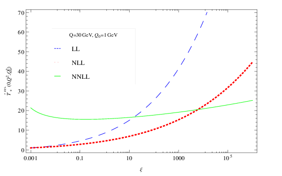
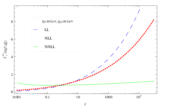
We have to make a choice for the scale , which, in principle, is arbitrary. We wish to choose it by optimizing the apparent convergence properties of the perturbative QCD expansion. To this end, we analyse in Figs. 1 and 2 the dependence on the scaling parameter of governed by Eq. (46) at different logarithmic accuracies for GeV and GeV, respectively. We put GeV because this is in the center of the range where the majority of the available data located. We observe a strong reduction of the scale dependence as we pass from LL via NLL to NNLL, both for GeV and GeV. The perturbative series appears to be more rapidly converging at relatively large values of . Therefore, we adopt GeV in the following. Another good reason for this choice is that, according to Eq. (61), and represent the avarage gluon and quark jet multiplicities, respectively, at the scale , so that the fit results for our initial conditions may be directly compared with the experimental data at GeV.
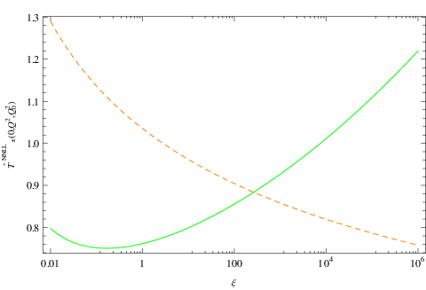
In Fig. 3, we compare the scale dependence of , which is obtained by simply replacing with in Eq. (41), with the one of evaluated according to Eq. (46), for GeV and GeV. We observe from Fig. 3 that the scale variation is very similar in both cases.
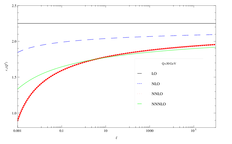
In Fig. 4, we study the scale dependence of evaluated at LO, NLO, NNLO, and N3LO according to Eq. (66). We observe that the scale dependence gradually increases as we pass from LO via NLO to NNLO, while it decreases in the step from NNLO to N3LO, and hence conclude that only the latter order may be trusted.
Prior to presenting our fits, we explain our definition of confidence level (CL), which we adopt from Ref. [43]. Suppose a fit of the free parameters to experimental data points yields the minimum value . We then determine the 90% CL limits on a fit parameter by varying it so that the resulting values stay within the range
| (67) |
where are defined such that
| (68) |
with
| (69) |
| 18.09 | 3.71 | 2.92 |
The average gluon and quark jet multiplicities extracted from experimental data strongly depend on the choice of jet algorithm. We adopt the selection of experimental data from Ref. [44] performed in such a way that they correspond to compatible jet algorithms. Specifically, these include the measurements of average gluon jet multiplicities in Refs. [44, 45, 46, 47, 48] and those of average quark jet multiplicities in Refs. [45, 49, 50, 51, 52, 53, 54, 55, 56, 57, 58, 59, 60, 61, 62, 63, 64, 65, 66, 67, 68, 69, 70, 71, 72, 73, 74, 75, 76, 77], which include 27 and 51 experimental data points, respectively. The results for and at GeV together with the values obtained in our , , and fits are listed in Table 1. The errors correspond to 90% CL as explained above. All these fit results are in agreement with the experimental data. Looking at the values, we observe that the qualities of the fits improve as we go to higher orders, as they should. The improvement is most dramatic in the step from to , where the errors on and are more than halved. The improvement in the step from to , albeit less pronounced, indicates that the inclusion of the first correction to as given in Eq. (54) is favored by the experimental data. We have verified that the values of are insensitive to the choice of , as they should. Furthermore, the central values converge in the sense that the shifts in the step from to are considerably smaller than those in the step from to and that, at the same time, the central values after each step are contained within error bars before that step. In the fits presented so far, the strong-coupling constant was taken to be the central value of the world avarage, [78]. In Section 5, we shall include among the fit parameters.
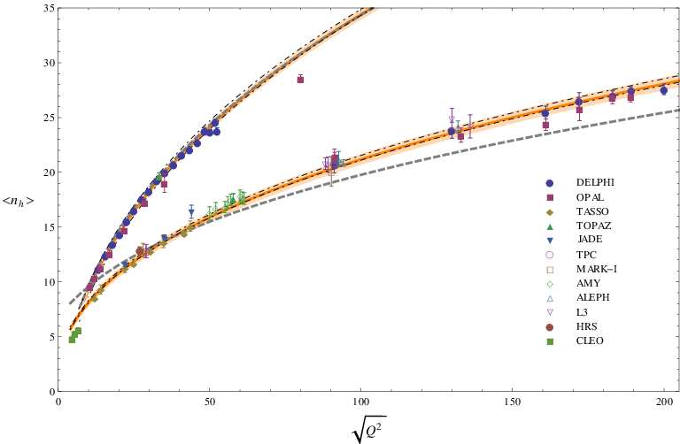


In Fig. 5, we show as functions of the average gluon and quark jet multiplicities evaluated from Eq. (57) at and using the corresponding fit results for and at GeV from Table 1. For clarity, we refrain from including in Fig. 5 the results, which are very similar to the ones already presented in Ref. [13]. In the case, Fig. 5 also displays two error bands, namely the experimental one induced by the 90% CL errors on the respective fit parameters in Table 1 and the theoretical one, which is evaluated from Eqs. (46) and (66) by varying the scale parameter in the range . For a more detailed discussion of the uncertainties on the average gluon and quark jet multiplicities in the approximation, we display them as functions of in Fig. 6 and 7, respectively, normalized with respect to the default results, evaluated with . We observe that the uncertainties decrease with increasing value of , which is a consequence of the asymptotic freedom of QCD. They typically fall below at GeV, but become significant at low values indicating the onset of the breakdown of the perturbative expansion in .


While our fits rely on individual measurements of the average gluon and quark jet multiplicities, the experimental literature also reports determinations of their ratio; see Refs. [11, 44, 46, 48, 79, 80, 81, 82, 83, 84, 85, 86, 87, 88, 89, 90, 91, 92, 93], which essentially cover all the available measurements. In order to find out how well our fits describe the latter and thus to test the global consistency of the individual measurements, we compare in Fig. 8 the experimental data on the average gluon-to-quark jet multiplicity ratio with our evaluations of Eq. (59) in the and approximations using the corresponding fit results from Table 1. As in Fig. 5, we present in Fig. 8 also the experimental and theoretical uncertainties in the result. As in Figs. 6 and 7, they are represented relative to the default result, with , in Fig. 9. For comparison, we include in Fig. 8 also the prediction of Ref. [9] given by Eq. (55).
Looking at Fig. 8, we observe that the experimental data are very well described by the result for values above 10 GeV, while they somewhat overshoot it below. This discrepancy is likely to be due to the fact that, following Ref. [44], we excluded the older data from Ref. [11] from our fits because they are inconsistent with the experimental data sample compiled in Ref. [44]. Furthermore, Fig. 9 tells us that the theoretical uncertainties are large in the small- region, which indicates that the convergence properties of the perturbative series in are unfavorable there. Finally, the experimental determination of the scale , which in the theoretical expressions denotes the virtuality of the parent parton of the considered jet, may be ambiguous in multi-jet events and may be performed somewhat differently in different experiments, which may explain tensions between different data sets. This additional type of uncertainty should be more important at small values of , where the slope of the evolution is steeper.
The Monte Carlo analysis of Ref. [10] suggests that the average gluon and quark jet multiplicities should coincide at about GeV. As is evident from Fig. 8, this agrees with our result reasonably well given the considerable uncertainties in the small- range discussed above.

As is obvious from Fig. 8, the approximation of by given in Eq. (55) [9] leads to a poor approximation of the experimental data, which reach up to values of about 50 GeV. It is, therefore, interesting to study the high- asymptotic behavior of the average gluon-to-quark jet ratio. This is done in Fig. 10, where the result including its experimental and theoretical uncertainties is compared with the approximation by Eq. (55) way up to TeV. We observe from Fig. 10 that the approximation approaches the result rather slowly. Both predictions agree within theoretical errors at TeV, which is one order of magnitude beyond LHC energies, where they are still about 10% below the asymptotic value . Figure 10 also nicely illustrates how, as a consequence of the asymptotic freedom of QCD, the theoretical uncertainty decreases with increasing value of and thus becomes considerably smaller than the experimental error.
5 Determination of strong-coupling constant
| 2.84 | 2.85 |
In Section 4, we took to be a fixed input parameter for our fits. Motivated by the excellent goodness of our and fits, we now include it among the fit parameters, the more so as the fits should be sufficiently sensitive to it in view of the wide range populated by the experimental data fitted to. We fit to the same experimental data as before and again put GeV. The fit results are summarized in Table 2. We observe from Table 2 that the results of the [42] and fits for and are mutually consistent. They are also consistent with the respective fit results in Table 1. As expected, the values of are reduced by relasing in the fits, from 3.71 to 2.84 in the approximation and from 2.95 to 2.85 in the one. The three-parameter fits strongly confine , within an error of 3.7% at 90% CL in both approximations. The inclusion of the term has the beneficial effect of shifting closer to the world average, [78]. In fact, our value, at 90% CL, which corresponds to at 68% CL, is in excellent agreement with the former.

6 Conclusions
Prior to our analysis in Ref. [13], experimental data on the average gluon and quark jet multiplicities could not be simultaneously described in a satisfactory way mainly because the theoretical formalism failed to account for the difference in hadronic contents between gluon and quark jets, although the convergence of perturbation theory seemed to be well under control [9]. This problem may be solved by including the minus components governed by in Eqs. (57) and (59). This was done for the first time in Ref. [13], albeit in connection with the LO result . The quark-singlet minus component comes with an arbitrary normalization and has a slow dependence. Consequently, its numerical contribution may be approximately mimicked by a constant introduced to the average quark jet multiplicity as in Ref. [11].
In the present paper, we improved the analysis of Ref. [13] in various ways. The most natural possible improvement consists in including higher-order correction to . Here, we managed to obtain the NLO correction, of , using the effective approach introduced in Ref. [12], which was shown to also exactly reproduce the correction to . Our general result corresponding to Eq. (57) depends on two parameters, and , which, according to Eq. (61), represent the average gluon and quark jet multiplicities at an arbitrary reference scale and act as initial conditions for the evolution. Looking at the perturbative behaviour of the expansion in and the distribution of the available experimental data, we argued that GeV is a good choice. We fitted these two parameters to all available experimental data on the average gluon and quark jet multiplicities treating as an input parameter fixed to the world avarage [78]. We worked in three different approximations, labeled , , and , in which the logarithms are resummed through the NNLL level, is evaluated at LO or approximately at N3LO, and is evaluated at LO or NLO. Including the NLO correction to , given in Eq. (54), significantly improved the quality of the fit, as is evident by comparing the values of for the and fits in Table 1.
Motivated by the goodness of our and fits with fixed value of in Ref. [13] and here, we then included among the fit parameters, which yielded a further reduction of . The fit results are listed in Table 2. Also here, the inclusion of the NLO correction to is beneficial; it shifts closer to the world average to become .
A few comments are in order regarding the renormalization scheme and the counting of higher-order corrections in our analysis in order to allow for an appropriate classification of our determination of in the context of a global analysis yielding a world average. We worked in the renormalization scheme, which has become the standard choice in the literature. We reach beyond ordinary fixed-order analyses by resumming the logarithms through the NNLL level. Furthermore, our expressions are completely RG-improved in the sense that all dependence is accommodated in . Unlike usual higher-order calculations in the QCD-improved parton model, the perturbation series of the coefficients are organized in powers of rather than . In the case of , which starts at , our exact knowledge reaches through , i.e. NNLO, while our term represents an educated guess in the sense that it was obtained using a procedure that, strictly speaking, was only tested through NNLO. In the case of , the term vanishes, and the term is listed in Eq. (54), i.e. we have control through NLO. However, the coefficients of in Eq. (57) are numerically suppressed relative to those of , by approximately a factor of . In fact, the shift in () induced by the term of is comparable to (about a factor of three smaller than) the one induced by the term of . We thus conclude that our determination of is effectively of NNLO.
The next steps towards accuracy include an improved computation of the coefficient and an extended resummation of the plus and minus components of the splitting functions. At the LHC, jet multiplicity observables can be measured at unprecedented values of , which will allow for stringent tests of QCD and provide a strong lever arm for high-precision determinations of using the formalism elaborated in Ref. [13] and here.
Acknowledgments
The work P.B. and of A.V.K. was supported in part by the Heisenberg-Landau program. The work of A.V.K. was supported in part by the Russian Foundation for Basic Research RFBR through Grant No. 13-02-01005. This work was supported by the German Federal Ministry for Education and Research BMBF through Grant No. 05H12GUE and by the German Research Foundation DFG through the Collaborative Research Centre No. 676 Particles, Strings and the Early Universe—The Structure of Matter and Space Time.
Appendix
Here we prove the relations given in Eqs. (29) and (30) between the singular parts of the diagonal and nondiagonal splitting functions in Mellin space with and show that they are approximately true also for the regular parts.
Following Ref. [6], we introduce the notation22 2 In order for all variables to be positive, we introduce here instead of used in Ref. [6].
| (70) |
In the following, the resummed functions are built up by their parts corresponding to the considered levels of resummation, with representing the LL, NLL, and NNLL levels, respectively. The results read:
| (71) |
where , , and
| (72) |
with .
Through NNLL accuracy, the nondiagonal splitting functions may be represented as
| (73) | |||||
| (74) |
where
| (75) |
with
| (76) |
We observe from Eq. (73) that the relation for the NNLL-resummed parts of the splitting functions and in Eq. (30) is not only correct for their terms singular as , but also for their regular ones. The situation is different for the relation between and in Eq. (29), which does not carry over to the regular terms, as is evident from Eq. (74). However, the additional terms in Eq. (75) have simple forms compared to the expression for in Eq. (71).
References
- [1] W. J. Waalewijn, Phys. Rev. D 86 (2012) 094030 [arXiv:1209.3019 [hep-ph]].
- [2] Ya. I. Azimov, Yu. L. Dokshitzer, V. A. Khoze and S. I. Troyan, Z. Phys. C 27 (1985) 65.
- [3] A. H. Mueller, Phys. Lett. B 104 (1981) 161.
- [4] A. Vogt, JHEP 1110 (2011) 025 [arXiv:1108.2993 [hep-ph]].
- [5] S. Albino, P. Bolzoni, B. A. Kniehl and A. V. Kotikov, Nucl. Phys. B 855 (2012) 801 [arXiv:1108.3948 [hep-ph]].
- [6] C.-H. Kom, A. Vogt and K. Yeats, JHEP 1210 (2012) 033 [arXiv:1207.5631 [hep-ph]].
- [7] S. Albino, P. Bolzoni, B. A. Kniehl and A. Kotikov, arXiv:1107.1142 [hep-ph].
- [8] S. Albino, P. Bolzoni, B. A. Kniehl and A. Kotikov, Nucl. Phys. B 851 (2011) 86 [arXiv:1104.3018 [hep-ph]].
- [9] A. Capella, I. M. Dremin, J. W. Gary, V. A. Nechitailo and J. Tran Thanh Van, Phys. Rev. D 61 (2000) 074009 [hep-ph/9910226].
- [10] P. Eden and G. Gustafson, JHEP 9809 (1998) 015 [hep-ph/9805228].
- [11] P. Abreu et al. [DELPHI Collaboration], Phys. Lett. B 449 (1999) 383 [hep-ex/9903073].
- [12] P. Bolzoni, arXiv:1206.3039 [hep-ph], DOI: 10.3204/DESY-PROC-2012-02/96.
- [13] P. Bolzoni, B. A. Kniehl and A. V. Kotikov, Phys. Rev. Lett. 109 (2012) 242002 [arXiv:1209.5914 [hep-ph]].
- [14] R. K. Ellis, W. J. Stirling and B. R. Webber, Camb. Monogr. Part. Phys. Nucl. Phys. Cosmol. 8 (1996) 1.
- [15] M. Glück, E. Reya and A. Vogt, Phys. Rev. D 48 (1993) 116 [Erratum-ibid. D 51 (1995) 1427].
- [16] S. Moch and A. Vogt, Phys. Lett. B 659 (2008) 290 [arXiv:0709.3899 [hep-ph]].
- [17] A. A. Almasy, S. Moch and A. Vogt, Nucl. Phys. B 854 (2012) 133 [arXiv:1107.2263 [hep-ph]].
- [18] A. J. Buras, Rev. Mod. Phys. 52 (1980) 199.
- [19] A. V. Kotikov and L. N. Lipatov, Nucl. Phys. B 661 (2003) 19 [Erratum-ibid. B 685 (2004) 405] [hep-ph/0208220].
- [20] B. I. Ermolaev and V. S. Fadin, Pis’ma Zh. Eksp. Teor. Fiz. 33 (1981) 285 [JETP Lett. 33 (1981) 269]
- [21] Yu. L. Dokshitzer, V. S. Fadin and V. A. Khoze, Z. Phys. C 15 (1982) 325.
- [22] Yu. L. Dokshitzer, V. S. Fadin and V. A. Khoze, Phys. Lett. B 115 (1982) 242.
- [23] Yu. L. Dokshitzer, V. S. Fadin and V. A. Khoze, Z. Phys. C 18 (1983) 37.
- [24] R. Kirschner and L. N. Lipatov, Zh. Eksp. Teor. Fiz. 83 (1982) 488 [Sov. Phys. JETP 56 (1982) 266].
- [25] R. Kirschner and L. N. Lipatov, Nucl. Phys. B 213 (1983) 122.
- [26] A. V. Kotikov and G. Parente, Nucl. Phys. B 549 (1999) 242 [hep-ph/9807249].
- [27] V. S. Fadin and L. N. Lipatov, Phys. Lett. B 429 (1998) 127 [hep-ph/9802290].
- [28] A. V. Kotikov and L. N. Lipatov, Nucl. Phys. B 582 (2000) 19 [hep-ph/0004008].
- [29] V. S. Fadin, E. A. Kuraev and L. N. Lipatov, Phys. Lett. B 60 (1975) 50.
- [30] E. A. Kuraev, L. N. Lipatov and V. S. Fadin, Zh. Eksp. Teor. Fiz. 71 (1976) 840 [Sov. Phys. JETP 44 (1976) 443].
- [31] E. A. Kuraev, L. N. Lipatov and V. S. Fadin, Zh. Eksp. Teor. Fiz. 72 (1977) 377 [Sov. Phys. JETP 45 (1977) 199].
- [32] I. I. Balitsky and L. N. Lipatov, Yad. Fiz. 28 (1978) 1597 [Sov. J. Nucl. Phys. 28 (1978) 822].
- [33] M. Ciafaloni, D. Colferai, G. P. Salam and A. M. Stasto, JHEP 0708 (2007) 046 [arXiv:0707.1453 [hep-ph]].
- [34] G. Altarelli, R. D. Ball and S. Forte, Nucl. Phys. B 799 (2008) 199 [arXiv:0802.0032 [hep-ph]].
- [35] A. H. Mueller, Nucl. Phys. B 241 (1984) 141.
- [36] M. Schmelling, Phys. Scripta 51 (1995) 683.
- [37] I. M. Dremin and J. W. Gary, Phys. Rept. 349 (2001) 301 [hep-ph/0004215].
- [38] A. Yu. Illarionov, A. V. Kotikov and G. Parente, Phys. Part. Nucl. 39 (2008) 307 [hep-ph/0402173].
- [39] G. Cvetic, A. Yu. Illarionov, B. A. Kniehl and A. V. Kotikov, Phys. Lett. B 679 (2009) 350 [arXiv:0906.1925 [hep-ph]].
- [40] I. M. Dremin and J. W. Gary, Phys. Lett. B 459 (1999) 341 [hep-ph/9905477].
- [41] Yu. L. Dokshitzer, V. A. Khoze, A. H. Mueller and S. I. Troyan, Basics of perturbative QCD, Editions Frontières, edited by J. Tran Thanh Van, (Fong and Sons Printers Pte. Ltd., Singapore, 1991).
- [42] P. Bolzoni, arXiv:1211.5550 [hep-ph].
- [43] D. Stump, J. Pumplin, R. Brock, D. Casey, J. Huston, J. Kalk, H. L. Lai and W. K. Tung, Phys. Rev. D 65 (2001) 014012 [hep-ph/0101051].
- [44] J. Abdallah et al. [DELPHI Collaboration], Eur. Phys. J. C 44 (2005) 311 [hep-ex/0510025].
- [45] K. Nakabayashi et al. [TOPAZ Collaboration], Phys. Lett. B 413 (1997) 447.
- [46] G. Abbiendi et al. [OPAL Collaboration], Eur. Phys. J. C 11 (1999) 217 [hep-ex/9903027].
- [47] G. Abbiendi et al. [OPAL Collaboration], Eur. Phys. J. C 37 (2004) 25 [hep-ex/0404026].
- [48] M. Siebel, Ph.D. Thesis No. WUB-DIS 2003-11, Bergische Universität Wuppertal, November 2003.
- [49] S. Kluth et al. [JADE Collaboration], hep-ex/0305023.
- [50] M. Althoff et al. [TASSO Collaboration], Z. Phys. C 22 (1984) 307.
- [51] W. Braunschweig et al. [TASSO Collaboration], Z. Phys. C 45 (1989) 193.
- [52] H. Aihara et al. [TPC/Two Gamma Collaboration], Phys. Lett. B 184 (1987) 299.
- [53] P. C. Rowson, G. Trilling, G. S. Abrams, D. Amidei, A. R. Baden, T. Barklow, A. Boyarski and J. Boyer et al., Phys. Rev. Lett. 54 (1985) 2580.
- [54] M. Derrick, K. K. Gan, P. Kooijman, J. S. Loos, B. Musgrave, L. E. Price, J. Repond and J. Schlereth et al., Phys. Rev. D 34 (1986) 3304.
- [55] H. W. Zheng et al. [AMY Collaboration], Phys. Rev. D 42 (1990) 737.
- [56] G. S. Abrams, C. Adolphsen, D. Averill, J. Ballam, B. C. Barish, T. Barklow, B. A. Barnett and J. E. Bartelt et al., Phys. Rev. Lett. 64 (1990) 1334.
- [57] D. Decamp et al. [ALEPH Collaboration], Phys. Lett. B 234 (1990) 209.
- [58] D. Decamp et al. [ALEPH Collaboration], Phys. Lett. B 273 (1991) 181.
- [59] D. Buskulic et al. [ALEPH Collaboration], Z. Phys. C 69 (1995) 15.
- [60] R. Barate et al. [ALEPH Collaboration], Phys. Rept. 294 (1998) 1.
- [61] P. Abreu et al. [DELPHI Collaboration], Z. Phys. C 50 (1991) 185.
- [62] P. Abreu et al. [DELPHI Collaboration], Z. Phys. C 52 (1991) 271.
- [63] B. Adeva et al. [L3 Collaboration], Phys. Lett. B 259 (1991) 199.
- [64] B. Adeva et al. [L3 Collaboration], Z. Phys. C 55 (1992) 39.
- [65] M. Z. Akrawy et al. [OPAL Collaboration], Z. Phys. C 47 (1990) 505.
- [66] P. D. Acton et al. [OPAL Collaboration], Phys. Lett. B 291 (1992) 503.
- [67] P. D. Acton et al. [OPAL Collaboration], Z. Phys. C 53 (1992) 539.
- [68] P. Abreu et al. [DELPHI Collaboration], Eur. Phys. J. C 5 (1998) 585.
- [69] K. Ackerstaff et al. [OPAL Collaboration], Eur. Phys. J. C 7 (1999) 369 [hep-ex/9807004].
- [70] M. Acciarri et al. [L3 Collaboration], Phys. Lett. B 371 (1996) 137.
- [71] P. Abreu et al. [DELPHI Collaboration], Phys. Lett. B 372 (1996) 172.
- [72] G. Alexander et al. [OPAL Collaboration], Z. Phys. C 72 (1996) 191.
- [73] D. Buskulic et al. [ALEPH Collaboration], Z. Phys. C 73 (1997) 409.
- [74] K. Ackerstaff et al. [OPAL Collaboration], Z. Phys. C 75 (1997) 193.
- [75] P. Abreu et al. [DELPHI Collaboration], Phys. Lett. B 416 (1998) 233.
- [76] G. Abbiendi et al. [OPAL Collaboration], Eur. Phys. J. C 16 (2000) 185 [hep-ex/0002012].
- [77] P. Abreu et al. [DELPHI Collaboration], Eur. Phys. J. C 18 (2000) 203 [Erratum-ibid. C 25 (2002) 493] [hep-ex/0103031].
- [78] J. Beringer et al. [Particle Data Group Collaboration], Phys. Rev. D 86 (2012) 010001.
- [79] M. S. Alam et al. [CLEO Collaboration], Phys. Rev. D 56 (1997) 17 [hep-ex/9701006].
- [80] H. Albrecht et al. [ARGUS Collaboration], Z. Phys. C 54 (1992) 13.
- [81] M. S. Alam et al. [CLEO Collaboration], Phys. Rev. D 46 (1992) 4822.
- [82] D. Acosta et al. [CDF Collaboration], Phys. Rev. Lett. 94 (2005) 171802.
- [83] M. Derrick, K. K. Gan, P. Kooijman, J. S. Loos, B. Musgrave, L. E. Price, J. Schlereth and K. Sugano et al., Phys. Lett. B 165 (1985) 449.
- [84] W. Braunschweig et al. [TASSO Collaboration], Z. Phys. C 45 (1989) 1.
- [85] G. Alexander et al. [OPAL Collaboration], Phys. Lett. B 265, 462 (1991).
- [86] P. D. Acton et al. [OPAL Collaboration], Z. Phys. C 58, 387 (1993).
- [87] R. Akers et al. [OPAL Collaboration], Z. Phys. C 68, 179 (1995).
- [88] O. Biebel [OPAL Collaboration], in DPF‘96: The Minneapolis Meeting, edited by K. Heller, J. K. Nelson, and D. Reeder (World Scientific Publishing Co. Pte. Ltd., Singapore, 1998), Volume 1, p. 354–356.
- [89] D. Buskulic et al. [ALEPH Collaboration], Phys. Lett. B 384 (1996) 353.
- [90] P. Abreu et al. [DELPHI Collaboration], Z. Phys. C 70 (1996) 179.
- [91] G. Alexander et al. [OPAL Collaboration], Phys. Lett. B 388 (1996) 659.
- [92] K. Ackerstaff et al. [OPAL Collaboration], Eur. Phys. J. C 1 (1998) 479 [hep-ex/9708029].
- [93] G. Abbiendi et al. [OPAL Collaboration], Phys. Rev. D 69 (2004) 032002 [hep-ex/0310048].