Two-dimensional arrays of superconducting and soft magnetic strips as dc magnetic metamaterials

We investigate 2D arrays of superconducting and soft magnetic strips as the basic components of dc magnetic metamaterials. The thickness, $d$, of the strips is much smaller than the width, and is regarded as infinitesimal, $\epsilon=d/2\to 0$. The length, $L_{z}$, of the strips along the $z$ axis is much larger than the width, and is regarded as infinite, $L_{z}\to\infty$. The wide surface of the strips is parallel to the $xz$ plane, and the strips are regularly arranged in the $xy$ plane. We analyze the local (microscopic) magnetic field, ${\bi H}=H_{x}(x,y)\hat{\bi x}+H_{y}(x,y)\hat{\bi y}$, in the $xy$ plane. Outside the strips, the relationship between the local magnetic field, ${\bi H}$, and the local magnetic induction, ${\bi B}=B_{x}(x,y)\hat{\bi x}+B_{y}(x,y)\hat{\bi y}$, is given by ${\bi B}=\mu_{0}{\bi H}$, where $\mu_{0}$ is the vacuum permeability.

The 2D magnetic field is analyzed using the complex field [11, 12]

$${\cal H}(\zeta)=H_{y}(x,y)+\rmi H_{x}(x,y),$$

(2.1)

as the analytic function of the complex variable $\zeta=x+\rmi y$. The complex potential is defined by ${\cal G}(\zeta)=\int{\cal H}(\zeta)\rmd\zeta$, and the contour lines of $\mbox{Re}\,{\cal G}(x+\rmi y)$ correspond to the magnetic field lines in the $xy$ plane.

In the unit cell of the 2D array, the macroscopic magnetic field $\langle\bi H\rangle$ is calculated as the averaged line integral of $\bi H$ at the cell edge, whereas the macroscopic magnetic permeability $\langle\bi B\rangle$ is calculated as the averaged surface integral of $\bi B$ at the cell side [10, 13, 14]. Because of the different definitions of the averaging procedure for obtaining the macroscopic fields, the macroscopic relationship, $\langle\bi B\rangle\neq\mu_{0}\langle\bi H\rangle$, generally holds, even though the microscopic relationship, ${\bi B}=\mu_{0}{\bi H}$, holds. We consider the case where the wide surfaces of the strips are parallel to the $xz$ plane; therefore the permeability tensor $\mu_{\alpha\beta}$ defined by $\langle B_{\alpha}\rangle=\mu_{\alpha\beta}\langle H_{\beta}\rangle$ has only diagonal components, $\mu_{xx}=\mu_{\parallel}$ and $\mu_{yy}=\mu_{\perp}$:

$$\langle B_{x}\rangle=\mu_{\parallel}\langle H_{x}\rangle\quad\mbox{and}\quad\langle B_{y}\rangle=\mu_{\perp}\langle H_{y}\rangle.$$

(2.2)

The magnetic response to a parallel field is characterized by the parallel permeability, $\mu_{\parallel}$, whereas the response to a perpendicular field is characterized by the perpendicular permeability, $\mu_{\perp}$. We demonstrate later that for superconducting strip arrays, $0<\mu_{\perp}/\mu_{0}\ll\mu_{\parallel}/\mu_{0}\simeq 1$, whereas for soft magnetic strip arrays, $\mu_{\parallel}/\mu_{0}\gg\mu_{\perp}/\mu_{0}\simeq 1$. We also show that for the hybrid arrays of superconducting and soft magnetic strips, $0<\mu_{\perp}/\mu_{0}\ll 1\ll\mu_{\parallel}/\mu_{0}$.

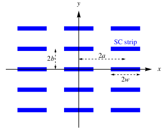
We consider a rectangular array of superconducting strips, in which the superconducting strips of width $2w$ are regularly arranged with a unit cell of $2a\times 2b$ in the $xy$ plane, as shown in figure 1.

We employ the auxiliary complex variable, $\eta_{r}$, defined as

$$\eta_{r}(\zeta)\equiv\mbox{sn}(\zeta/c_{r},k_{r}),$$

(3.1)

where $\mbox{sn}(u,k)$ is the sine amplitude (i.e., the Jacobi sn function) [16]. The modulus, $k_{r}$, is obtained as a function of $b/a$ by solving

$$b/a={\bf K}(\sqrt{1-k_{r}^{2}})/{\bf K}(k_{r}),$$

(3.2)

where ${\bf K}(k)$ is the complete elliptic integral of the first kind [16]. The $c_{r}$ in (3.1) is then given by

$$c_{r}=a/{\bf K}(k_{r})=b/{\bf K}(\sqrt{1-k_{r}^{2}}).$$

(3.3)

The complex field ${\cal H}(\zeta)$ and the complex potential ${\cal G}(\zeta)=\int_{ib}^{\zeta}{\cal H}(\zeta^{\prime})\rmd\zeta^{\prime}$ for the rectangular array of superconducting strips in the complete shielding state are  [10]

	$\displaystyle{\cal H}(\zeta)$	$\displaystyle=H_{0y}\frac{\eta_{r}(\zeta)}{\sqrt{\eta_{r}(\zeta)^{2}-\gamma_{r}^{2}}}+\rmi H_{0x},$			(3.4)
	$\displaystyle{\cal G}(\zeta)$	$\displaystyle=\frac{H_{0y}c_{r}}{\sqrt{1-k_{r}^{2}\gamma_{r}^{2}}}\,F\left(\arcsin\sqrt{\frac{k_{r}^{-2}-\gamma_{r}^{2}}{\eta_{r}(\zeta)^{2}-\gamma_{r}^{2}}},\kappa_{r}\right)+\rmi H_{0x}\zeta,$			(3.5)

where $F(\varphi,k)$ is the elliptic integral of the first kind [16]. The parameters $\gamma_{r}$ and $\kappa_{r}$ in (3.4) and (3.5) are defined as

	$\displaystyle\gamma_{r}$	$\displaystyle=\eta_{r}(w)=\mbox{sn}(w/c_{r},k_{r}),$			(3.6)
	$\displaystyle\kappa_{r}$	$\displaystyle=\sqrt{\frac{1-\gamma_{r}^{2}}{k_{r}^{-2}-\gamma_{r}^{2}}}=\frac{k_{r}\mbox{cn}(w/c_{r},k_{r})}{\mbox{dn}(w/c_{r},k_{r})},$			(3.7)

where $\mbox{cn}(u,k)$ and $\mbox{dn}(u,k)$ are the Jacobi cn and dn functions, respectively. We do not need to consider the details of the constants $H_{0y}$ and $H_{0x}$ in (3.4) and (3.5), because neither $H_{0x}$ nor $H_{0y}$ affects the final results of the effective permeability [17].

When the rectangular array of superconducting strips is exposed to a parallel magnetic field along the $x$ axis, the magnetic field is not disturbed by thin superconducting strips where $\epsilon\to 0$; that is, (3.4) shows that ${\cal H}(\zeta)=\rmi H_{0x}$ for $H_{0y}=0\neq H_{0x}$. In this case, the macroscopic fields are $\langle B_{x}\rangle/\mu_{0}=\langle H_{x}\rangle=H_{0x}$, and the macroscopic permeability for a parallel field is equal to the vacuum permeability, $\mu_{\parallel}/\mu_{0}=1$, for the thin-strip limit.

In contrast, when the rectangular array of superconducting strips is exposed to a perpendicular magnetic field along the $y$ axis (i.e., $H_{0x}=0\neq H_{0y}$), the magnetic field is disturbed by the superconducting strips. Because of the magnetic shielding by the superconducting strips, the macroscopic permeability for a perpendicular field is smaller than the vacuum permeability, $0<\mu_{\perp}/\mu_{0}<1$, depending on the geometry of the 2D array. Figure 2 shows the magnetic field lines as the contour lines of $\mbox{Re}\,{\cal G}(x+\rmi y)$ obtained from (3.5) for $H_{0x}=0$. The magnetic field is concentrated near the gaps between the edges of the superconducting strips.

The local magnetic induction, $B_{y}(x,y)=\mu_{0}H_{y}(x,y)$, and the local magnetic field, $H_{y}(x,y)=\mbox{Re}\,{\cal H}(x+\rmi y)$, are obtained from (3.4). We examine the macroscopic perpendicular fields, $\langle B_{y}\rangle$ and $\langle H_{y}\rangle$, averaged over the unit cell of the rectangular array. The macroscopic magnetic induction $\langle B_{y}\rangle$ and macroscopic magnetic field $\langle H_{y}\rangle$ are calculated from the local fields as [10]

	$\displaystyle\frac{\langle B_{y}\rangle}{\mu_{0}}$	$\displaystyle\equiv\frac{1}{2a}\int_{-a}^{+a}H_{y}(x,b)\rmd x=\frac{1}{2a}\int_{-a}^{+a}H_{y}(x,y)\rmd x,$			(3.8)
	$\displaystyle\langle H_{y}\rangle$	$\displaystyle\equiv\frac{1}{2b}\int_{0}^{2b}H_{y}(a,y)\rmd y.$			(3.9)

The last expression of (3.8) is independent of $y$, because $\nabla\cdot{\bi B}=0$ [10]. As shown in A.1, the macroscopic fields defined by (3.8) and (3.9) are consistent with the macroscopic relationship,

$$\langle B_{y}\rangle/\mu_{0}=\langle H_{y}\rangle+\langle M_{y}\rangle,$$

(3.10)

where $\langle M_{y}\rangle$ is the magnetization of superconducting strips defined by

$$\langle M_{y}\rangle\equiv-\frac{1}{4ab}\int_{-w}^{+w}xK_{z}(x)\rmd x$$

(3.11)

and $K_{z}(x)=H_{x}(x,-\epsilon)-H_{x}(x,+\epsilon)$ is the sheet current density in superconducting strips.

The macroscopic perpendicular permeability $\mu_{\rm\perp sc,r}=\langle B_{y}\rangle/\langle H_{y}\rangle$ for the rectangular array of superconducting strips is obtained from (3.4), (3.8), and (3.9), as

$$\frac{\mu_{\perp\rm sc,r}}{\mu_{0}}=\frac{b}{a}\frac{{\bf K}(\kappa_{r})}{{\bf K}(\sqrt{1-\kappa_{r}^{2}})},$$

(3.12)

where $\kappa_{r}$ is given by (3.7). Simple expressions of $\mu_{\perp\rm sc,r}$ for limiting cases can be obtained from (3.12). For a large stack spacings, $b/a>2$,

$$\frac{\mu_{\perp\rm sc,r}}{\mu_{0}}\simeq\left[1-\frac{2a}{\pi b}\ln\cos\left(\frac{\pi w}{2a}\right)\right]^{-1},$$

(3.13)

whereas for small stack spacings, $b/a\ll 1$,

$$\frac{\mu_{\perp\rm sc,r}}{\mu_{0}}\simeq 1-\frac{w}{a}+\frac{2b}{\pi a}\ln 2.$$

(3.14)

Equation (3.14) is not accurate near $w/a\simeq 0$ or $1$. Figure 3 shows plots of $\mu_{\perp\rm sc,r}/\mu_{0}$ versus $w/a$ obtained from (3.2), (3.3), (3.7), and (3.12). We can obtain a small perpendicular permeability, $\mu_{\perp\rm sc,r}/\mu_{0}\ll 1$, when the gaps between the edges of the superconducting strips are small, $1-w/a\ll 1$.

We next consider a hexagonal array of superconducting strips, in which the superconducting strips of width $2w$ are regularly arranged in the $xy$ plane, as shown in figure 4.

We employ the auxiliary complex variable, $\eta_{h}$, defined as

$$\eta_{h}(\zeta)\equiv\mbox{sn}(\zeta/c_{h},k_{h}).$$

(3.15)

The modulus, $k_{h}$, is obtained as a function of $b/a$ by solving

$$2b/a={\bf K}(\sqrt{1-k_{h}^{2}})/{\bf K}(k_{h}).$$

(3.16)

The relationship between $k_{h}$ defined by (3.16) and $k_{r}$ defined by (3.2) is expressed by $k_{h}=(1-\sqrt{1-k_{r}^{2}})/(1+\sqrt{1-k_{r}^{2}})$. The value of $c_{h}$ in (3.15) is given by

$$c_{h}=a/{\bf K}(k_{h})=2b/{\bf K}(\sqrt{1-k_{h}^{2}}).$$

(3.17)

The complex field ${\cal H}(\zeta)$ and the complex potential ${\cal G}(\zeta)=\int_{ib}^{\zeta}{\cal H}(\zeta^{\prime})\rmd\zeta^{\prime}$ for the rectangular array of superconducting strips in the complete shielding state are [10]

	$\displaystyle{\cal H}(\zeta)$	$\displaystyle=H_{0y}\frac{\eta_{h}(\zeta)\sqrt{\eta_{h}(\zeta)^{2}-k_{h}^{-2}}}{\sqrt{\eta_{h}(\zeta)^{2}-\gamma_{h}^{2}}\sqrt{\eta_{h}(\zeta)^{2}-\beta_{h}^{2}}}+\rmi H_{0x},$			(3.18)
	$\displaystyle{\cal G}(\zeta)$	$\displaystyle=\frac{H_{0y}c_{h}}{k_{h}\sqrt{\beta_{h}^{2}-\gamma_{h}^{2}}}\,F\left(\arcsin\sqrt{\frac{\beta_{h}^{2}-\gamma_{h}^{2}}{\eta_{h}(\zeta)^{2}-\gamma_{h}^{2}}},\kappa_{h}\right)+\rmi H_{0x}\zeta,$			(3.19)

where

	$\displaystyle\gamma_{h}$	$\displaystyle=\eta_{h}(w)=\mbox{sn}(w/c_{h},k_{h}),$			(3.20)
	$\displaystyle\beta_{h}$	$\displaystyle=\eta_{h}(a-w+2\rmi b)=\sqrt{\frac{k_{h}^{-2}-\gamma_{h}^{2}}{1-\gamma_{h}^{2}}}=\frac{\mbox{dn}(w/c_{h},k_{h})}{k_{h}\mbox{cn}(w/c_{h},k_{h})}.$			(3.21)
	$\displaystyle\kappa_{h}$	$\displaystyle=\left[\frac{(1-\gamma_{h}^{2})^{2}}{k_{h}^{-2}-1+(1-\gamma_{h}^{2})^{2}}\right]^{1/2}=\left[1+\frac{k_{h}^{-2}-1}{\mbox{cn}^{4}(w/c_{h},k_{h})}\right]^{-1/2}.$			(3.22)

Under a parallel magnetic field along the $x$ axis, (3.18) shows that ${\cal H}(\zeta)=\rmi H_{0x}$ for $H_{0y}=0\neq H_{0x}$, and the macroscopic permeability for a parallel field is equal to the vacuum permeability, $\mu_{\parallel}/\mu_{0}=1$, for the thin-strip limit.

In contrast, under a perpendicular magnetic field along the $y$ axis (i.e., $H_{0x}=0\neq H_{0y}$), the magnetic field is disturbed by the superconducting strips. Figure 5 shows the magnetic field lines as the contour lines of $\mbox{Re}\,{\cal G}(x+\rmi y)$ obtained from (3.19) for $H_{0x}=0$. The magnetic field is concentrated near the gaps between the edges of the superconducting strips.

The definitions of the macroscopic magnetic induction $\langle B_{y}\rangle$ and the magnetization $\langle M_{y}\rangle$ for the hexagonal array are the same as those for the rectangular array, and are expressed by (3.8) and (3.11), respectively. The definition of the macroscopic magnetic field for the hexagonal array, $\langle H_{y}\rangle$, given by (3.9) is inconsistent with the macroscopic relationship given by (3.10). Therefore, we use the modified definition of $\langle H_{y}\rangle$ for the hexagonal array [10],

$$\langle H_{y}\rangle\equiv\frac{1}{2b}\left[\int_{0}^{2b}H_{y}(a,y)\rmd y-\int_{0}^{a}H_{x}(x,2b-\epsilon)\rmd x\right].$$

(3.23)

For the hexagonal array, the macroscopic quantities defined by (3.8), (3.11), and (3.23) satisfy (3.10), as shown in A.2.

The macroscopic perpendicular permeability, $\mu_{\rm\perp sc,h}=\langle B_{y}\rangle/\langle H_{y}\rangle$, for the hexagonal array of superconducting strips, is obtained from (3.8), (3.18), and (3.23):

$$\frac{\mu_{\perp\rm sc,h}}{\mu_{0}}=\frac{2b}{a}\frac{{\bf K}(\kappa_{h})}{{\bf K}(\sqrt{1-\kappa_{h}^{2}})}.$$

(3.24)

Here $\kappa_{h}$ is given by (3.22). For large stack spacings, $b/a>2$, the right-hand side of (3.24) also reduces to the right-hand side of (3.13). For small stack spacings, $b/a\ll 1$,

$$\frac{\mu_{\perp\rm sc,h}}{\mu_{0}}\simeq\cases{1-\frac{2w}{a}+\frac{8b}{\pi a}\ln 2&for $\displaystyle 0<w/a<1/2$\\ \left(\frac{2b}{a}\right)^{2}\left(\frac{2w}{a}-1+\frac{8b}{\pi a}\ln 2\right)^{-1}&for $1/2<w/a<1$}.$$

(3.25)

Equation (3.25) is not accurate near $w/a\simeq 0$, $1/2$ or $1$. Figure 6 shows plots of $\mu_{\perp\rm sc,h}/\mu_{0}$ versus $w/a$ obtained from (3.16), (3.17), (3.22), and (3.24). We can obtain a small perpendicular permeability, $\mu_{\perp\rm sc,h}/\mu_{0}\ll 1$, for a wide range of $0.5<w/a<1$, when $b/a\ll 1$.

We consider a rectangular array of soft magnetic strips, in which soft magnetic strips of width $2w$ are regularly arranged with a unit cell of $2a\times 2b$ in the $xy$ plane, as shown in figure 7. The geometry of the rectangular array of soft magnetic strips is exactly the same as that of the rectangular array of superconducting strips shown in figure 1.

The complex field, ${\cal H}(\zeta)$, and the complex potential, ${\cal G}(\zeta)=\int_{ib}^{\zeta}{\cal H}(\zeta^{\prime})\rmd\zeta^{\prime}$, for the rectangular array of soft magnetic strips based on the ideal soft magnet model are given by

	$\displaystyle{\cal H}(\zeta)$	$\displaystyle=H_{0y}+\rmi\,H_{0x}\frac{\eta_{r}(\zeta)}{\sqrt{\eta_{r}(\zeta)^{2}-\gamma_{r}^{2}}},$			(4.1)
	$\displaystyle{\cal G}(\zeta)$	$\displaystyle=H_{0y}\zeta+\frac{\rmi\,H_{0x}c_{r}}{\sqrt{1-k_{r}^{2}\gamma_{r}^{2}}}\,F\left(\arcsin\sqrt{\frac{k_{r}^{-2}-\gamma_{r}^{2}}{\eta_{r}(\zeta)^{2}-\gamma_{r}^{2}}},\kappa_{r}\right),$			(4.2)

where $\eta_{r}$, $k_{r}$, $c_{r}$, $\gamma_{r}$, and $\kappa_{r}$ are defined by (3.1), (3.2), (3.3), (3.6), and (3.7), respectively. The behavior of the soft magnetic strips is analogously dual to that of the superconducting strips; (4.1) and (4.2) are obtained simply by exchanging $H_{0y}\leftrightarrow\rmi H_{0x}$ in (3.4) and (3.5), respectively [20].

When the rectangular array of soft magnetic strips is exposed to a perpendicular magnetic field along the $y$ axis, the magnetic field is not disturbed by thin soft magnetic strips where $\epsilon\to 0$; that is, (4.1) shows that ${\cal H}(\zeta)=H_{0y}$ for $H_{0x}=0\neq H_{0y}$. In this case, the macroscopic fields are $\langle B_{y}\rangle/\mu_{0}=\langle H_{y}\rangle=H_{0y}$, and the macroscopic permeability for a perpendicular field is equal to the vacuum permeability, $\mu_{\perp}/\mu_{0}=1$, for the thin-strip limit.

In contrast, when the rectangular array of soft magnetic strips is exposed to a parallel magnetic field along the $x$ axis (i.e., $H_{0y}=0\neq H_{0x}$), the magnetic field is disturbed by the soft magnetic strips. The macroscopic permeability for a parallel field is larger than the vacuum permeability, $\mu_{\parallel}/\mu_{0}>1$, depending on the geometry of the 2D array. Figure 8 shows the magnetic field lines as the contour lines of $\mbox{Re}\,{\cal G}(x+\rmi y)$ obtained from (4.2) for $H_{0y}=0$.

The macroscopic parallel fields, $\langle B_{x}\rangle$ and $\langle H_{x}\rangle$, averaged over the unit cell of the rectangular array are defined by

	$\displaystyle\frac{\langle B_{x}\rangle}{\mu_{0}}$	$\displaystyle\equiv\frac{1}{2b}\int_{0}^{2b}H_{x}(a,y)\rmd y,$			(4.3)
	$\displaystyle\langle H_{x}\rangle$	$\displaystyle\equiv\frac{1}{2a}\int_{-a}^{+a}H_{x}(x,b)\rmd x=\frac{1}{2a}\int_{-a}^{+a}H_{x}(x,y)\rmd x.$			(4.4)

The last expression of (4.4) is independent of $y$, because $\nabla\times{\bi H}=0$ [10]. As shown in A.3, (4.3) and (4.4) are consistent with

$$\langle B_{x}\rangle/\mu_{0}=\langle H_{x}\rangle+\langle M_{x}\rangle,$$

(4.5)

where $\langle M_{x}\rangle$ is the magnetization arising from the soft magnetic strips, defined as [10]

$$\langle M_{x}\rangle\equiv\frac{1}{4ab}\int_{-w}^{+w}x\sigma_{m}(x)\rmd x.$$

(4.6)

The expression $\sigma_{m}(x)=H_{y}(x,+\epsilon)-H_{y}(x,-\epsilon)$ corresponds to the effective sheet magnetic charge in the soft magnetic strips [18, 19].

The macroscopic parallel permeability, $\mu_{\rm\parallel sm,r}=\langle B_{x}\rangle/\langle H_{x}\rangle$, for the rectangular array of soft magnetic strips is obtained from (4.1), (4.3), and (4.4), as

$$\frac{\mu_{\parallel\rm sm,r}}{\mu_{0}}=\frac{a}{b}\frac{{\bf K}(\sqrt{1-\kappa_{r}^{2}})}{{\bf K}(\kappa_{r})},$$

(4.7)

where $\kappa_{r}$ is given by (3.7). Note that $\mu_{\perp\rm sc,r}$ given by (3.12) and $\mu_{\parallel\rm sm,r}$ given by (4.7) hold the simple relationship $\mu_{\parallel\rm sm,r}=\mu_{0}^{2}/\mu_{\perp\rm sc,r}$. Figure 3 shows plots of $\mu_{0}/\mu_{\parallel\rm sm,r}$ versus $w/a$ obtained from (3.2), (3.3), (3.7), and (4.7). We can obtain a large parallel permeability, $\mu_{\parallel\rm sm,r}/\mu_{0}\gg 1$, when the gaps between the edges of the soft magnetic strips are small, $1-w/a\ll 1$.

We next consider a hexagonal array of soft magnetic strips, in which soft magnetic strips of width $2w$ are regularly arranged with a unit cell of $2a\times 2b$ in the $xy$ plane, as shown in figure 9. The geometry of the hexagonal array of soft magnetic strips is exactly the same as that of the hexagonal array of superconducting strips shown in figure 4.

The complex field, ${\cal H}(\zeta)$, and the complex potential ${\cal G}(\zeta)=\int_{ib}^{\zeta}{\cal H}(\zeta^{\prime})\rmd\zeta^{\prime}$ for the hexagonal array of soft magnetic strips based on the ideal soft magnet model are given by

	$\displaystyle{\cal H}(\zeta)$	$\displaystyle=H_{0y}+\rmi\,H_{0x}\frac{\eta_{h}(\zeta)\sqrt{\eta_{h}(\zeta)^{2}-k_{h}^{-2}}}{\sqrt{\eta_{h}(\zeta)^{2}-\gamma_{h}^{2}}\sqrt{\eta_{h}(\zeta)^{2}-\beta_{h}^{2}}},$			(4.8)
	$\displaystyle{\cal G}(\zeta)$	$\displaystyle=H_{0y}\zeta+\frac{\rmi\,H_{0x}c_{h}}{k_{h}\sqrt{\beta_{h}^{2}-\gamma_{h}^{2}}}\,F\left(\arcsin\sqrt{\frac{\beta_{h}^{2}-\gamma_{h}^{2}}{\eta_{h}(\zeta)^{2}-\gamma_{h}^{2}}},\kappa_{h}\right),$			(4.9)

where $\eta_{h}$, $k_{h}$, $c_{h}$, $\gamma_{h}$, $\beta_{h}$, and $\kappa_{h}$ are defined by (3.15), (3.16), (3.17), (3.20), (3.21), and (3.22), respectively. Equation (4.8) and (4.9) are obtained simply by exchanging $H_{0y}\leftrightarrow\rmi H_{0x}$ in (3.18) and (3.19), respectively.

When the hexagonal array of soft magnetic strips is exposed to a perpendicular magnetic field along the $y$ axis, (4.8) shows that ${\cal H}(\zeta)=H_{0y}$ for $H_{0x}=0\neq H_{0y}$. The macroscopic permeability for a perpendicular field is equal to the vacuum permeability, $\mu_{\perp}/\mu_{0}=1$, for the thin-strip limit.

In contrast, when the hexagonal array of soft magnetic strips is exposed to a parallel magnetic field along the $x$ axis ($H_{0x}\neq 0$ and $H_{0y}=0$), the magnetic field is disturbed by the soft magnetic strips. Figure 10 shows the magnetic field lines as the contour lines of $\mbox{Re}\,{\cal G}(x+\rmi y)$ obtained from (4.9).

The definitions of the macroscopic magnetic field, $\langle H_{x}\rangle$, and the magnetization, $\langle M_{x}\rangle$, for the hexagonal array are the same as those used for the rectangular array, and are given by (4.4) and (4.6), respectively. However, the definition of the macroscopic magnetic induction, $\langle B_{x}\rangle$, for the hexagonal array given by (4.3) is inconsistent with the macroscopic relationship given by (4.5). Therefore, we use the modified definition of $\langle B_{x}\rangle$ for the hexagonal array,

$$\frac{\langle B_{x}\rangle}{\mu_{0}}\equiv\frac{1}{2b}\left[\int_{0}^{2b}H_{x}(a,y)\rmd y+\int_{0}^{a}H_{y}(x,2b-\epsilon)\rmd x\right].$$

(4.10)

For the hexagonal array, the macroscopic quantities defined by (4.4), (4.6), and (4.10) satisfy (4.5), as shown in A.4.

The macroscopic parallel permeability, $\mu_{\rm\parallel sm,h}=\langle B_{x}\rangle/\langle H_{x}\rangle$, for the hexagonal array of soft magnetic strips is obtained from (4.4), (4.8), and (4.10), as

$$\frac{\mu_{\parallel\rm sm,h}}{\mu_{0}}=\frac{a}{2b}\frac{{\bf K}(\sqrt{1-\kappa_{h}^{2}})}{{\bf K}(\kappa_{h})},$$

(4.11)

where $\kappa_{h}$ is given by (3.22). Note that $\mu_{\perp\rm sc,h}$ given by (3.24) and $\mu_{\parallel\rm sm,h}$ given by (4.11) hold the simple relationship $\mu_{\parallel\rm sm,h}=\mu_{0}^{2}/\mu_{\perp\rm sc,h}$. Figure 6 shows plots of $\mu_{0}/\mu_{\perp\rm sm,h}$ versus $w/a$ obtained from (3.16), (3.17), (3.22), and (3.24). We can obtain a large parallel permeability, $\mu_{\parallel\rm sm,h}/\mu_{0}\gg 1$, for a wide range of $0.5<w/a<1$, when $b/a\ll 1$

We consider the hybrid array shown in figure 11, which is composed of the rectangular array of superconducting strips shown in figure 1 and the rectangular array of soft magnetic strips shown in figure 7.

The complex field ${\cal H}(\zeta)$ for the hybrid rectangular array of superconducting and soft magnetic strips is given by

$${\cal H}(\zeta)=H_{0y}\frac{\eta_{r}(\zeta)}{\sqrt{\eta_{r}(\zeta)^{2}-\gamma_{rs}^{2}}}+\rmi\,H_{0x}\frac{\eta_{r}(\zeta-a)}{\sqrt{\eta_{r}(\zeta-a)^{2}-\gamma_{rm}^{2}}},$$

(5.1)

where $\gamma_{rs}=\eta_{r}(w_{s})=\mbox{sn}(w_{s}/c_{r},k_{r})$, $\gamma_{rm}=\eta_{r}(w_{m}-a)=\mbox{cn}(w_{m}/c_{r},k_{r})/\mbox{dn}(w_{m}/c_{r},k_{r})$, and $\eta_{r}(\zeta)$ is given by (3.1). Equation (5.1) corresponds to the combination of (3.4) and (4.1). In a perpendicular magnetic field, $H_{0x}=0\neq H_{0y}$, the field distribution is determined by the arrangement of superconducting strips, and is not affected by the thin soft magnetic strips. In a parallel magnetic field, $H_{0y}=0\neq H_{0x}$, on the other hand, the field distribution is determined by the arrangement of soft magnetic strips, and is not affected by the thin superconducting strips.

The resulting macroscopic permeability for a perpendicular field $\mu_{\perp\rm hyb,r}$ and that for a parallel field $\mu_{\parallel\rm hyb,r}$ are respectively given by

	$\displaystyle\frac{\mu_{\perp\rm hyb,r}}{\mu_{0}}$	$\displaystyle=\frac{b}{a}\frac{{\bf K}(\kappa_{rs})}{{\bf K}(\sqrt{1-\kappa_{rs}^{2}})},$			(5.2)
	$\displaystyle\frac{\mu_{\parallel\rm hyb,r}}{\mu_{0}}$	$\displaystyle=\frac{a}{b}\frac{{\bf K}(\sqrt{1-\kappa_{rm}^{2}})}{{\bf K}(\kappa_{rm})},$			(5.3)

where $\kappa_{rs}=k_{r}\mbox{cn}(w_{s}/c_{r},k_{r})/\mbox{dn}(w_{s}/c_{r},k_{r})$ and $\kappa_{rm}=k_{r}\mbox{cn}(w_{m}/c_{r},k_{r})/\mbox{dn}(w_{m}/c_{r},k_{r})$. For small stack periodicity, $b/a\ll 1$, (5.2) and (5.3) reduce to

	$\displaystyle\frac{\mu_{\perp\rm hyb,r}}{\mu_{0}}$	$\displaystyle\simeq 1-\frac{w_{s}}{a}+\frac{2b}{\pi a}\ln 2,$			(5.4)
	$\displaystyle\frac{\mu_{\parallel\rm hyb,r}}{\mu_{0}}$	$\displaystyle\simeq\left(1-\frac{w_{m}}{a}+\frac{2b}{\pi a}\ln 2\right)^{-1}.$			(5.5)

Equation (5.4) is not accurate near $w_{s}/a\simeq 0$ or $1$, and (5.5) is not accurate near $w_{m}/a\simeq 0$ or $1$. If $w_{s}=w_{m}=a/2$ and $b/a\ll 1$, then $\mu_{\perp\rm hyb,r}/\mu_{0}\simeq\mu_{0}/\mu_{\parallel\rm hyb,r}\simeq 1/2$. Figure 12 shows plots of $\mu_{\perp\rm hyb,r}/\mu_{0}$ and $\mu_{\parallel\rm hyb,r}/\mu_{0}$ versus $w_{s}/a=1-w_{m}/a$ for the case where $w_{s}+w_{m}=a$, calculated from (5.2) and (5.3).

We next consider the hybrid array shown in figure 13, which is composed of the hexagonal array of superconducting strips shown in figure 4 and the hexagonal array of soft magnetic strips shown in figure 9.

The complex field ${\cal H}(\zeta)$ for the hybrid hexagonal array of superconducting and soft magnetic strips is given by

	$\displaystyle{\cal H}(\zeta)=$	$\displaystyle H_{0y}\frac{\eta_{h}(\zeta)\sqrt{\eta_{h}(\zeta)^{2}-k_{h}^{-2}}}{\sqrt{\eta_{h}(\zeta)^{2}-\gamma_{hs}^{2}}\sqrt{\eta_{h}(\zeta)^{2}-\beta_{hs}^{2}}}$			(5.6)
		$\displaystyle+\rmi\,H_{0x}\frac{\eta_{h}(\zeta-a)\sqrt{\eta_{h}(\zeta-a)^{2}-k_{h}^{-2}}}{\sqrt{\eta_{h}(\zeta-a)^{2}-\gamma_{hm}^{2}}\sqrt{\eta_{h}(\zeta-a)^{2}-\beta_{hm}^{2}}},$

where $\gamma_{hs}=\eta_{h}(w_{s})=\mbox{sn}(w_{s}/c_{h},k_{h})$, $\gamma_{hm}=\eta_{h}(w_{m}-a)=\mbox{cn}(w_{m}/c_{h},k_{h})/\mbox{dn}(w_{m}/c_{h},k_{h})$, and $\eta_{h}(\zeta)$ is given by (3.15). Equation (5.6) corresponds to the combination of (3.18) and (4.8). In a perpendicular magnetic field, $H_{0x}=0\neq H_{0y}$, the field distribution is determined by the arrangement of superconducting strips, and is not affected by the thin soft magnetic strips. In a parallel magnetic field, $H_{0y}=0\neq H_{0x}$, on the other hand, the field distribution is determined by the arrangement of soft magnetic strips, and is not affected by the thin superconducting strips.

The resulting macroscopic permeability for a perpendicular field, $\mu_{\perp}$, and that for a parallel field, $\mu_{\parallel}$, are given by

	$\displaystyle\frac{\mu_{\perp\rm hyb,h}}{\mu_{0}}$	$\displaystyle=\frac{2b}{a}\frac{{\bf K}(\kappa_{hs})}{{\bf K}(\sqrt{1-\kappa_{hs}^{2}})},$			(5.7)
	$\displaystyle\frac{\mu_{\parallel\rm hyb,h}}{\mu_{0}}$	$\displaystyle=\frac{a}{2b}\frac{{\bf K}(\sqrt{1-\kappa_{hm}^{2}})}{{\bf K}(\kappa_{hm})},$			(5.8)

respectively, where

	$\displaystyle\kappa_{hs}$	$\displaystyle=\left[1+\frac{k_{h}^{-2}-1}{\mbox{cn}^{4}(w_{s}/c_{h},k_{h})}\right]^{-1/2},$			(5.9)
	$\displaystyle\kappa_{hm}$	$\displaystyle=\left[1+\frac{k_{h}^{-2}-1}{\mbox{cn}^{4}(w_{m}/c_{h},k_{h})}\right]^{-1/2},$			(5.10)

For a small stack periodicity, $b/a\ll 1$, (5.7) and (5.8) reduce to

$$\frac{\mu_{\perp\rm hyb,h}}{\mu_{0}}\simeq\cases{1-\frac{2w_{s}}{a}+\frac{8b}{\pi a}\ln 2&for $\displaystyle 0<w_{s}/a<1/2$\\ \left(\frac{2b}{a}\right)^{2}\left(\frac{2w_{s}}{a}-1+\frac{8b}{\pi a}\ln 2\right)^{-1}&for $1/2<w_{s}/a<1$},$$

(5.11)

$$\frac{\mu_{\parallel\rm hyb,h}}{\mu_{0}}\simeq\cases{\left(1-\frac{2w_{m}}{a}+\frac{8b}{\pi a}\ln 2\right)^{-1}&for $\displaystyle 0<w_{m}/a<1/2$\\ \left(\frac{a}{2b}\right)^{2}\left(\frac{2w_{m}}{a}-1+\frac{8b}{\pi a}\ln 2\right)&for $1/2<w_{m}/a<1$}.$$

(5.12)

Equation (5.11) is not accurate near $w_{s}/a\simeq 0$, $1/2$, or $1$, and (5.12) is not accurate near $w_{m}/a\simeq 0$, $1/2$, or $1$. If $w_{s}=w_{m}=a/2$ and $b/a\ll 1$, then $\mu_{\perp\rm hyb,h}/\mu_{0}\simeq\mu_{0}/\mu_{\parallel\rm hyb,h}\simeq 2b/a\ll 1$. Figure 14 shows plots of $\mu_{\perp\rm hyb,h}/\mu_{0}$ and $\mu_{\parallel\rm hyb,h}/\mu_{0}$ versus $w_{s}/a=1-w_{m}/a$ for the case where $w_{s}+w_{m}=a$, calculated from (5.7) and (5.8).

References

- [1] Wood B and Pendry J B 2007 Metamaterials at zero frequency J. Phys.: Condens. Matter19 076208
- [2] Magnus F, Wood B, Moore J, Morrison K, Perkins G, Fyson J, Wiltshire M C K, Caplin D, Cohen L F and Pendry J B 2008 A d.c. magnetic metamaterial Nature Mater. 7 295
- [3] Navau C, Chen D-X, Sanchez A and Del-Valle N 2009 Magnetic properties of a dc metamaterial consisting of parallel square superconducting thin plates Appl. Phys. Lett. 94 242501
- [4] Cummer S A, Popa B-I, Schurig D and Smith D R 2006 Full-wave simulations of electromagnetic cloaking structures Phys. Rev. E 74 036621
- [5] Schurig D, Mock J J, Justice B J, Cummer S A, Pendry J B, Starr A F, and Smith D R 2006 Metamaterial Electromagnetic Cloak at Microwave Frequencies Science 314 977–980
- [6] Yaghjian A D and Maci S 2008 Alternative derivation of electromagnetic cloaks and concentrators New J. Phys.10 115022
- [7] Sanchez A, Navau C, Prat-Camps J, and Chen D-X 2011 Antimagnets: controlling magnetic fields with superconductor-metamaterial hybrids New J. Phys.13 093034
- [8] Narayana S and Sato Y 2011 DC Magnetic Cloak Advanced Materials 24 71–74
- [9] Gömöry F, Solovyov M, Šouc J, Navau C, Prat-Camps J and Sanchez A 2012 Experimental Realization of a Magnetic Cloak Science 335 1466–1468
- [10] Mawatari Y, Navau C and Sanchez A 2012 Two-dimensional arrays of superconducting strips as dc magnetic metamaterials Phys. Rev.B 85 134524
- [11] Landau L D and Lifschitz E M 1963 Electrodynamics of Continuous Media, Theoretical Physics (Pergamon, Oxford, 1963), Vol. 8
- [12] Beth R A 1966 Complex representation and computation of two-dimensional magnetic fields J. Appl. Phys.37 2568
- [13] Pendry J B, Holden A J, Robbins D J and Stewart W J 1999 Magnetism from conductors and enhanced nonlinear phenomena IEEE Trans. Microwave Theory Tech. 47 2075
- [14] Smith D R and Pendry J B 2006 Homogenization of metamaterials by field averaging J. Opt. Soc. Am. B 23 391
- [15] Bean C P (1962). Magnetization of hard superconductors. Phys. Rev. Lett., 8, 250-253.
- [16] Gradshtein I S and Ryzhik I M 1994 Table of Integrals, Series, and Products, 5th ed., (Academic, New York)
- [17] For linear magnetic materials investigated in the present paper (i.e., superconducting strips in the complete shielding state or ideal soft magnetic strips), neither nor affects the effective permeability. If we consider the nonliner magnetic response (e.g., superconducting strips in the critical state), the and need to be determined as functions of and . The relationship between the complex field at and the applied field may be determined by considering the total shape (e.g., the demagnetizaition factor) of magnetic metamaterials.
- [18] Mawatari Y 2008 Magnetic field distributions around superconducting strips on ferromagnetic substrates Phys. Rev. B 77 104505
- [19] Jackson J D 1975 Classical Electrodynamics, 2nd ed., (Wiley, New York)
- [20] Chen D-X, Prados C, Pardo E, Sanchez A and Hernando A 2002 Transverse demagnetizing factors of long rectangular bars: I. Analytical expressions for extreme values of susceptibility J. Appl. Phys.91 5254
- [21] We do not investigate the case when soft magnetic strips are vertical to superconducting strips, because the anisotropy in the macroscopic permeability is weak for such vertical hybrid arrays.
- [22] Gömöry F, Vojenčiak M, Pardo E, Solovyov M and Šouc J 2010 AC losses in coated conductors Supercond. Sci. Technol.23 034012