跳到论文正文
W Papers独立论文阅读器 arXiv:1305.5152 论文正文 计算阅读时间 · 0%
引用这篇论文根据当前论文元数据生成,正式投稿前建议核对。


License: arXiv.org perpetual non-exclusive license
arXiv:1305.5152v2 [hep-ph] 03 Mar 2014

Threshold resummation for the production of a color sextet (antitriplet) scalar at the LHC

Yong Chuan Zhan Affiliation: Department of Physics and State Key Laboratory of Nuclear Physics and Technology, Peking University, Beijing, 100871, China    Ze Long Liu Affiliation: Department of Physics and State Key Laboratory of Nuclear Physics and Technology, Peking University, Beijing, 100871, China    Shi Ang Li Affiliation: Department of Physics and State Key Laboratory of Nuclear Physics and Technology, Peking University, Beijing, 100871, China    Chong Sheng Li Note: Electronic address: csli@pku.edu.cn Affiliation: Department of Physics and State Key Laboratory of Nuclear Physics and Technology, Peking University, Beijing, 100871, China Affiliation: Center for High Energy Physics, Peking University, Beijing, 100871, China    Hai Tao Li Affiliation: Department of Physics and State Key Laboratory of Nuclear Physics and Technology, Peking University, Beijing, 100871, China
Abstract

ABSTRACT: We investigate threshold resummation effects in the production of a color sextet (antitriplet) scalar at next-to-next-to-leading logarithmic (NNLL) order at the LHC in the frame of soft-collinear effective theory. We show the total cross section and the rapidity distribution with NLO+NNLL accuracy, and we compare them with the NLO results. Besides, we use recent dijet data at the LHC to give the constraints on the couplings between the colored scalars and quarks.

pacs
12.38.Bx,12.38.Cy,14.65.Jk

I Introduction

There is no clear evidence of new physics beyond the Standard Model found at the LHC so far [1, 2, 3], and the most favored supersymmetry, extra dimensions, and many others all receive somewhat strong constraints [1, 4, 5]. Then it is a preferable way to be more concerned about the model independent theory rather than considering some specific models. Here we study the model independent color sextet (antitriplet) scalars, which have many significant effects in the phenomenology. Actually, color sextet scalars have been included in many new physics models, such as unification theories [6, 7, 8], supersymmetry with R-parity violation [9], and diquark Higgs [10]. Their masses can be as low as the TeV scale or less [11], which leads to much impact on the physics. For example, in the supersymmetric Pati-Salam S​U​(2)R×S​U​(2)L×S​U​(4)CSU(2)_{R}\times SU(2)_{L}\times SU(4)_{C} model, light color sextet scalars can be realized around the weak scale even though the scale of S​U​(2)R×S​U​(4)CSU(2)_{R}\times SU(4)_{C} symmetry breaking is around 101010^{10} GeV [11, 10]. Observation of the color sextet scalars will be a direct signal of new physics beyond the Standard Model.

Considering the interaction of the color sextet (antitriplet) scalars with quarks, which is parameterized, the relevant Lagrangian can be written as [12]

ℒ=22[K¯ia​bϕiψ¯a.(λLPL+λRPR).ψbC+h.c.]+(Dμi​jϕj)†Dμi​kϕk−mϕ2ϕi†ϕi,\mathcal{L}=2\sqrt{2}\left[\bar{K}_{i}^{ab}\phi^{i}\bar{\psi}_{a}.(\lambda_{L}P_{L}+\lambda_{R}P_{R}).\psi_{b}^{C}+h.c.\right]+(D_{\mu}^{ij}\phi_{j})^{\dagger}D_{\mu}^{ik}\phi_{k}-m_{\phi}^{2}\phi^{i\dagger}\phi^{i}, (1)

where Kia​bK_{i}^{ab} is the Clebsch-Gordan coefficient of the sextet (antitriplet), λL/R\lambda_{L/R} is the Yukawa-like coupling, and a,ba,b are the color indices. The quantum numbers of the colored scalars are listed in Table 1, and more information can be found in [12, 13].

 S​U​(2)LSU(2)_{L}  U​(1)YU(1)_{Y}  |Q|=|T3+Y||Q|=|T_{3}+Y|  couplings to
1 1/31/3 1/31/3 QQ,UD
3 1/31/3 1/3,2/3,4/31/3,2/3,4/3 QQ
1 −2/3-2/3 2/32/3 DD
1 4/34/3 4/34/3 UU
Table 1: Q is the S​U​(2)LSU(2)_{L} quark doublet, and U(D) is the up(down)-type S​U​(2)LSU(2)_{L} quark singlet. Under S​U​(3)C×S​U​(2)L×U​(1)YSU(3)_{C}\times SU(2)_{L}\times U(1)_{Y}, Q has the quantum numbers (3,2,1/61/6), while U has (3,1,2/32/3), and D has (3,1,−1/3-1/3).

In order to satisfy the gauge symmetry, the colored scalars couple to same-sign quarks, and then they have fractional electronic charges. In the cases of antitriplet the couplings should be antisymmetric in flavor. For convenience, we label the colored scalars as s​e​x​t​e​tIsextet^{I}, s​e​x​t​e​tI​Isextet^{II} and s​e​x​t​e​tI​I​Isextet^{III} with electronic charge 1/31/3, −2/3-2/3 and 4/34/3, respectively. For the antitriplet, the labels are a​n​t​i​t​r​i​p​l​e​tIantitriplet^{I}, a​n​t​i​t​r​i​p​l​e​tI​Iantitriplet^{II} and a​n​t​i​t​r​i​p​l​e​tI​I​Iantitriplet^{III}.

It has been shown [10, 14, 15] that the measurements of D0−D¯0D^{0}-\bar{D}^{0} mixing and the rate of D→π+​π0​(π+​ϕ)D\to\pi^{+}\pi^{0}(\pi^{+}\phi) decay can constrain the couplings of the colored scalars to two up-type quarks: λRu​u,λRu​c≲0.1,|Re(λc​cλuu∗)|∼5.76×10⁻⁷\lambda_{R}^{uu},\lambda_{R}^{uc}\lesssim 0.1,|Re(\lambda^{cc}\lambda^{uu*})|\sim 5.76\times 10^{-7} for mϕ∼m_{\phi}\sim 1 TeV. Besides, the left-handed coupling λL\lambda_{L} also receives a tight constraint due to minimal flavor violation. Since we use the model independent coupling λ2=λL2+λR2\lambda^{2}=\lambda_{L}^{2}+\lambda_{R}^{2}, above constraints can be relaxed in the scenario considered below.

Production and decay of the colored scalars at hadron colliders have been extensively discussed in [15, 12, 16, 17, 18, 19, 20]. Recently the CMS collaboration has searched for the signal of the colored scalar and obtained limits on the production cross section of such resonant states [21, 22, 23] with the fixed-order theoretical predictions (leading order and next-to-leading order) in Ref. [24, 18]. In this paper we investigate the threshold resummation effects in the single production of the color sextet (antitriplet) scalars, and we also discuss the rapidity distribution of the colored scalars at NLO+NNLL accuracy at the LHC with soft-collinear effective theory (SCET) [25, 26, 27, 28, 29]. As a cross check, we also calculate the NLO corrections using the analytical-phase space integral method, and present their analytical expressions. Actually, when the masses of the colored scalars approach the threshold limit, there are large logarithms left after cancelling the divergences, because the scale of the soft gluon radiations is rather small compared to the scalar mass. These threshold logarithms should be resummed to reduce the scale uncertainties and improve the confidence of the theoretical predictions.

This paper is organized as follows: In Sect. II, we present the NLO calculations. In Sect. III, we briefly show the factorization in the threshold limit of the production of the colored scalar. In Sect. IV, we calculate the soft function and present solutions of the renormalization group equations obeyed by hard and soft functions. In Sect. V, we present detailed numerical analyses and compare the NLO+NNLL rapidity distributions with the NLO results. We also use recent dijet data at the LHC to give constraints on the couplings between the colored scalars and quarks. We conclude in Sect. VI.

II Fixed-order calculations

We consider the process h1+h2→ϕ+Xh_{1}+h_{2}\rightarrow\phi+X, where h1h_{1} and h2h_{2} are the incoming hadrons with momenta P1P_{1} and P2P_{2}, and we define the rapidity of the colored scalar ϕ\phi as Y=12​ln⁡E+pzE−pzY=\frac{1}{2}\ln\frac{E+p_{z}}{E-p_{z}}, where EE and pzp_{z} represent the energy and longitudinal momentum of the scalar in the center-of-mass frame of the colliding hadrons. We write the cross section as [30, 31]:

d​σd​Y=∑i​j∫τ1d​zz​∫01d​y​fi/h1​(x1,μf)​fj/h2​(x2,μf)​Ci​j​(y,z,mϕ,μf),\frac{d\sigma}{dY}=\sum_{ij}\int_{\tau}^{1}\frac{dz}{z}\int_{0}^{1}dy\ f_{i/h_{1}}(x_{1},\mu_{f})f_{j/h_{2}}(x_{2},\mu_{f})C_{ij}(y,z,m_{\phi},\mu_{f}), (2)
Ci​j​(y,z,mϕ,μf)=z​|d​x1​d​x2d​y​d​z|​d​σi​jd​Y=12​S​∫d​P​Sf​|ℳi​j|2¯​δ​(y−u′−z(1−z)​(1+u′)),C_{ij}(y,z,m_{\phi},\mu_{f})=z\left|\frac{dx_{1}dx_{2}}{dydz}\right|\frac{d\sigma_{ij}}{dY}=\frac{1}{2S}\int d\!\ P\!S_{f}\ \overline{|\mathcal{M}_{ij}|^{2}}\ \delta\left(y-\frac{u^{\prime}-z}{(1-z)(1+u^{\prime})}\right), (3)

with

S=(P1+P2)2,τ=mϕ2/S,s=(p1+p2)2=x1​x2​S,\displaystyle S=(P_{1}+P_{2})^{2},\quad\tau=m_{\phi}^{2}/S,\quad s=(p_{1}+p_{2})^{2}=x_{1}x_{2}S,
u′=x1x2​e−2​Y,z=mϕ2s=τx1​x2,y=u′−z(1−z)​(1+u′),\displaystyle u^{\prime}=\frac{x_{1}}{x_{2}}e^{-2Y},\quad z=\frac{m_{\phi}^{2}}{s}=\frac{\tau}{x_{1}x_{2}},\quad y=\frac{u^{\prime}-z}{(1-z)(1+u^{\prime})}, (4)

where P​SfP\!S_{f} is the final state phase space, and μf\mu_{f} is the factorization scale. For one-particle final state, there is no yy dependence, and then the delta function can be reduced to (δ⁡(y)+δ⁡(1−y))/2(\delta(y)+\delta(1-y))/2.

The NLO corrections were investigated in Ref. [12] using the phase-space slicing method [32, 33]. Here we recalculate the matrix elements, which are consistent with the results in Ref. [12], and we do not present the details of these calculations. Below we just show the analytical expressions of the phase-space integration. Using the identity

x−1+ϵ=1ϵ​δ​(x)+∑nϵnn!​[lnn⁡xx]+,x^{-1+\epsilon}=\frac{1}{\epsilon}\delta(x)+\sum_{n}\frac{\epsilon^{n}}{n!}\left[\frac{\ln^{n}x}{x}\right]_{+}, (5)

with

∫τ1d​x​[lnn⁡(1−x)1−x]+​f​(x)=∫τ1d​x​lnn⁡(1−x)1−x​[f⁡(x)−f⁡(1)]−f⁡(1)​∫0τd​x​lnn⁡(1−x)1−x,\int_{\tau}^{1}dx\left[\frac{\ln^{n}(1-x)}{1-x}\right]_{+}f(x)=\int_{\tau}^{1}dx\frac{\ln^{n}(1-x)}{1-x}[f(x)-f(1)]-f(1)\int_{0}^{\tau}dx\frac{\ln^{n}(1-x)}{1-x}, (6)

we can obtain the following results for Ci​j​(y,z,mϕ,μf)C_{ij}(y,z,m_{\phi},\mu_{f}). The leading-order result is

Cq​q(0)=2​π​λ2​NDNC2​S​δ⁡(y)+δ⁡(1−y)2​δ​(1−z),C_{qq}^{(0)}=\frac{2\pi\lambda^{2}N_{D}}{N_{C}^{2}S}\frac{\delta(y)+\delta(1-y)}{2}\delta(1-z), (7)

and the contributions from the virtual and real corrections for the q​qqq channel are given by

Cq​qv​i​r​t\displaystyle C_{qq}^{virt} =\displaystyle= 2​π​λ2​NDNC2​Sδ⁡(y)+δ⁡(1−y)2δ(1−z)αs4​π(4​π)ϵΓ⁡(1−ϵ)[−4​CFϵ2+1ϵ(−2CD−6CF+4CFL)\displaystyle\frac{2\pi\lambda^{2}N_{D}}{N_{C}^{2}S}\frac{\delta(y)+\delta(1-y)}{2}\ \delta(1-z)\frac{\alpha_{s}}{4\pi}\frac{(4\pi)^{\epsilon}}{\Gamma(1-\epsilon)}\left[\frac{-4C_{F}}{\epsilon^{2}}+\frac{1}{\epsilon}(-2C_{D}-6C_{F}+4C_{F}L)\right. (8)
+CD(2L−2−4​π23)+CF(−2L2−4+2π2)]\displaystyle\left.+C_{D}\left(2L-2-\frac{4\pi^{2}}{3}\right)+C_{F}\left(-2L^{2}-4+2\pi^{2}\right)\right]

and

Cq​qr​e​a​l\displaystyle C_{qq}^{real} =\displaystyle= 2​π​λ2​NDNC2​Sαs4​π(4​π)ϵΓ⁡(1−ϵ){δ⁡(y)+δ⁡(1−y)2δ(1−z)4​CFϵ2\displaystyle\frac{2\pi\lambda^{2}N_{D}}{N_{C}^{2}S}\frac{\alpha_{s}}{4\pi}\frac{(4\pi)^{\epsilon}}{\Gamma(1-\epsilon)}\left\{\frac{\delta(y)+\delta(1-y)}{2}\delta(1-z)\frac{4C_{F}}{\epsilon^{2}}\right. (9)
+δ⁡(y)+δ⁡(1−y)2​1ϵ​((2​CD−4​CF​L)​δ​(1−z)−8​CF​[11−z]++4​CF​(1+z))\displaystyle+\frac{\delta(y)+\delta(1-y)}{2}\frac{1}{\epsilon}\left((2C_{D}-4C_{F}L)\delta(1-z)-8C_{F}\left[\frac{1}{1-z}\right]_{+}+4C_{F}(1+z)\right)
+CD​[δ⁡(y)+δ⁡(1−y)2​δ​(1−z)​(−2​L+4)−4​[11−z]++2​z+2]\displaystyle+C_{D}\left[\frac{\delta(y)+\delta(1-y)}{2}\delta(1-z)(-2L+4)-4\left[\frac{1}{1-z}\right]_{+}+2z+2\right]
+CFδ⁡(y)+δ⁡(1−y)2[δ(1−z)(2L2−2​π23)+8(L−ln(z))[11−z]+\displaystyle+C_{F}\frac{\delta(y)+\delta(1-y)}{2}\left[\delta(1-z)\left(2L^{2}-\frac{2\pi^{2}}{3}\right)+8\big(L-\ln(z)\big)\left[\frac{1}{1-z}\right]_{+}\right.
+16[ln⁡(1−z)1−z]+−4(1+z)(L+2ln(1−z)−ln(z))+4(1−z)]\displaystyle\left.+16\left[\frac{\ln(1-z)}{1-z}\right]_{+}-4(1+z)\big(L+2\ln(1-z)-\ln(z)\big)+4(1-z)\right]
+CF([1y]++[11−y]+)(4[11−z]+−2(1+z))},\displaystyle\left.+C_{F}\left(\left[\frac{1}{y}\right]_{+}+\left[\frac{1}{1-y}\right]_{+}\right)\left(4\left[\frac{1}{1-z}\right]_{+}-2(1+z)\right)\right\},

respectively. Combining the contributions of the LO results, the virtual and real corrections, we obtain the bare NLO partonic differential cross sections:

Cq​qb​a​r​e=Cq​q(0)+Cq​qv​i​r​t+Cq​qr​e​a​l.C_{qq}^{bare}=C_{qq}^{(0)}+C_{qq}^{virt}+C_{qq}^{real}. (10)

They still contain the collinear singularities, which can be factorized into the following form to all orders of perturbation theory in general:

Ci​jb​a​r​e​(z,1/ϵ)=∑k,lΓk​i​(z,μf,1/ϵ)⊗Γl​j​(z,μf,1/ϵ)⊗Ck​l​(z,μf),C_{ij}^{bare}(z,1/\epsilon)=\sum_{k,l}\Gamma_{ki}(z,\mu_{f},1/\epsilon)\otimes\Gamma_{lj}(z,\mu_{f},1/\epsilon)\otimes C_{kl}(z,\mu_{f}), (11)

where μf\mu_{f} is the factorization scale and ⊗\otimes is the convolution symbol defined as

f⁡(z)⊗g⁡(z)=∫z1d​yy​f​(y)​g​(zy).f(z)\otimes g(z)=\int_{z}^{1}\frac{dy}{y}f(y)g(\frac{z}{y}). (12)

The universal splitting functions Γi​j​(z,μf,1/ϵ)\Gamma_{ij}(z,\mu_{f},1/\epsilon) represent the probability of finding a particle ii with fraction zz of the longitudinal momentum inside the parent particle jj at the scale μf\mu_{f}. They contain the collinear divergences, and they can be absorbed into the redefinition of the PDF according to mass factorization [34, 35]. Adopting the M​S¯\overline{M\!S} mass-factorization scheme, we have to 𝒪⁡(αs)\mathcal{O}(\alpha_{s})

Γi​j​(z,μf,1/ϵ)=δi​j​δ​(1−z)−1ϵ​αs2​π​Γ⁡(1−ϵ)Γ⁡(1−2​ϵ)​(4​π​μr2μf2)ϵ​Pi​j(0)​(z),\Gamma_{ij}(z,\mu_{f},1/\epsilon)=\delta_{ij}\delta(1-z)-\frac{1}{\epsilon}\frac{\alpha_{s}}{2\pi}\frac{\Gamma(1-\epsilon)}{\Gamma(1-2\epsilon)}\left(\frac{4\pi\mu_{r}^{2}}{\mu_{f}^{2}}\right)^{\epsilon}P_{ij}^{(0)}(z), (13)

where Pi​j(0)​(z)P_{ij}^{(0)}(z) are the leading-order Altarelli-Parisi splitting functions [36]

Pq​q(0)​(z)\displaystyle P_{qq}^{(0)}(z) =\displaystyle= 43​[1+z2(1−z)++32​δ​(1−z)],\displaystyle\frac{4}{3}\left[\frac{1+z^{2}}{(1-z)_{+}}+\frac{3}{2}\delta(1-z)\right],
Pq​g(0)​(z)\displaystyle P_{qg}^{(0)}(z) =\displaystyle= 12​[(1−z)2+z2].\displaystyle\frac{1}{2}[(1-z)^{2}+z^{2}]. (14)

After absorbing the splitting functions Γi​j​(z,μf,1/ϵ)\Gamma_{ij}(z,\mu_{f},1/\epsilon) into the redefinition of the PDFs through the mass factorization in this way, we have the hard-scattering partonic differential cross sections Ci​j​(y,z,mϕ,μf)C_{ij}(y,z,m_{\phi},\mu_{f}), which are free of collinear divergences, and depend on the scale μf\mu_{f}. The final NLO results for the q​qqq channel are given by

Cq​q(1)\displaystyle C_{qq}^{(1)} =\displaystyle= 2​π​λ2​NDNC2​Sα​s4​π{δ⁡(y)+δ⁡(1−y)2[δ(1−z)(CD(2−43π2)+CF(43π2−4))\displaystyle\frac{2\pi\lambda^{2}N_{D}}{N_{C}^{2}S}\frac{\alpha s}{4\pi}\bigg\{\frac{\delta(y)+\delta(1-y)}{2}\bigg[\delta(1-z)\bigg(C_{D}\big(2-\frac{4}{3}\pi^{2}\big)+C_{F}\big(\frac{4}{3}\pi^{2}-4\big)\bigg) (15)
−8​CF​(ln⁡z−L)​[11−z]++16​CF​[ln⁡(1−z)1−z]+−4​CF​((z+1)​L+2​(z+1)​ln⁡(1−z)CLOSE\displaystyle-8C_{F}(\ln z-L)\bigg[\frac{1}{1-z}\bigg]_{+}+16C_{F}\bigg[\frac{\ln(1-z)}{1-z}\bigg]_{+}-4C_{F}\bigg((z+1)L+2(z+1)\ln(1-z)
−(z+1)lnz+z−1)]−2CF[1y]+(−2[11−z]++z+1)\displaystyle-(z+1)\ln z+z-1\bigg)\bigg]-2C_{F}\bigg[\frac{1}{y}\bigg]_{+}\bigg(-2\bigg[\frac{1}{1-z}\bigg]_{+}+z+1\bigg)
−2CF[11−y]+(−2[11−z]++z+1)+2CD(−2[11−z]++z+1)}.\displaystyle-2C_{F}\bigg[\frac{1}{1-y}\bigg]_{+}\bigg(-2\bigg[\frac{1}{1-z}\bigg]_{+}+z+1\bigg)+2C_{D}\bigg(-2\bigg[\frac{1}{1-z}\bigg]_{+}+z+1\bigg)\bigg\}.

Similarly, the final NLO result for the q​gqg channel is given by

Cq​g(1)\displaystyle C_{qg}^{(1)} =\displaystyle= 2​π​λ2​NDNC​(NC2−1)​Sαs4​π{δ(1−y)2CF[(2z2−2z+1)(L+2ln(1−z)−lnz−1)+1]\displaystyle\frac{2\pi\lambda^{2}N_{D}}{N_{C}(N_{C}^{2}-1)S}\frac{\alpha_{s}}{4\pi}\bigg\{\delta(1-y)2C_{F}\bigg[(2z^{2}-2z+1)\big(L+2\ln{(1-z)}-\ln{z}-1\big)+1\bigg] (16)
+2CF[11−y]+(2z2−2z+1)+2​(1−z)(y​z−y−z)2[CD(y2(z−1)2+z2)\displaystyle+2C_{F}\bigg[\frac{1}{1-y}\bigg]_{+}(2z^{2}-2z+1)+\frac{2(1-z)}{(yz-y-z)^{2}}\bigg[C_{D}\big(y^{2}(z-1)^{2}+z^{2}\big)
+CF(y+1)(z−1)(yz−y−z)2]},\displaystyle+C_{F}(y+1)(z-1)(yz-y-z)^{2}\bigg]\bigg\},

where λ2=λL2+λR2\lambda^{2}=\lambda_{L}^{2}+\lambda_{R}^{2}, L=ln⁡(mϕ2/μf2)L=\ln(m_{\phi}^{2}/\mu_{f}^{2}). The color factors are ND=6,CD=10/3N_{D}=6,C_{D}=10/3 for the sextet and ND=3,CD=4/3N_{D}=3,C_{D}=4/3 for the antitriplet. In the above results, we have set the renormalization scale μr=μf\mu_{r}=\mu_{f}. Finally, we combine these finite results to arrive at the NLO differential cross section Ci​j​(y,z,mϕ,μf)C_{ij}(y,z,m_{\phi},\mu_{f}) for colored scalar production:

Ci​j=Cq​q(0)+Cq​q(1)+Cq​g(1).C_{ij}=C_{qq}^{(0)}+C_{qq}^{(1)}+C_{qg}^{(1)}. (17)

Following the method in [30], we rearrange the results as

Cq​q​(z,y,mϕ,μf)=Cq​q(0)+Cq​q(1)=2​π​NDS​NC2​δ⁡(y)+δ⁡(1−y)2​C​(z,mϕ,μf)+Cq​qsubleading,C_{qq}(z,y,m_{\phi},\mu_{f})=C_{qq}^{(0)}+C_{qq}^{(1)}=\frac{2\pi N_{D}}{SN_{C}^{2}}\frac{\delta(y)+\delta(1-y)}{2}C(z,m_{\phi},\mu_{f})+C_{qq}^{\text{subleading}}, (18)

where the C⁡(z,mϕ,μf)C(z,m_{\phi},\mu_{f}) are the leading singular terms (threshold terms), which are arranged as

C⁡(z,mϕ,μf)\displaystyle C(z,m_{\phi},\mu_{f}) =\displaystyle= λ2δ[1−z]+λ2αs4​π{δ[1−z][CD(2−43π2)+CF(−4+43π2)]\displaystyle\lambda^{2}\delta[1-z]+\lambda^{2}\frac{\alpha_{s}}{4\pi}\bigg\{\delta[1-z]\left[C_{D}\left(2-\frac{4}{3}\pi^{2}\right)+C_{F}\left(-4+\frac{4}{3}\pi^{2}\right)\right] (19)
+[11−z]+[−4CD+8CF(L−lnz)]+[ln⁡(1−z)1−z]+16CF}.\displaystyle+\left[\frac{1}{1-z}\right]_{+}\big[-4C_{D}+8C_{F}(L-\ln z)\big]+\left[\frac{\ln(1-z)}{1-z}\right]_{+}16C_{F}\bigg\}.

From Eq. (19), we can see that the singular terms make the perturbative series badly convergent in the threshold limit z→1z\rightarrow 1, and thus they must be resummed to all orders.

III Factorization at threshold in SCET

The production of the colored scalar involves several scales, which are

s,mϕ2≫s​(1−z)2≫ΛQ​C​D2s,m_{\phi}^{2}\gg s(1-z)^{2}\gg\Lambda_{QCD}^{2} (20)

in the threshold limit, and it is convenient to introduce two light-like vectors nn and n¯\bar{n} along the directions of the colliding partons, which satisfy n⋅n¯=2n\cdot\bar{n}=2. In the lab frame, they can be written as

n=(1,0,0,1),n¯=(1,0,0,−1).n=(1,0,0,1),\quad\bar{n}=(1,0,0,-1). (21)

Then any four vector can be decomposed as

kμ=n⋅k​n¯μ2+n¯⋅k​nμ2+k⟂μ≡k+​n¯μ2+k−​nμ2+k⟂μ.k^{\mu}=n\cdot k\frac{\bar{n}^{\mu}}{2}+\bar{n}\cdot k\frac{n^{\mu}}{2}+k_{\perp}^{\mu}\equiv k^{+}\frac{\bar{n}^{\mu}}{2}+k^{-}\frac{n^{\mu}}{2}+k_{\perp}^{\mu}. (22)

In this limit, we need to distinguish four different momentum regions

hard: kμ∼s​(1,1,1),\displaystyle k^{\mu}\sim\sqrt{s}(1,1,1),
hard-collinear: kμ∼s​(ϵ,1,ϵ),\displaystyle k^{\mu}\sim\sqrt{s}(\epsilon,1,\sqrt{\epsilon}),
anti-hard-collinear: kμ∼s​(1,ϵ,ϵ),\displaystyle k^{\mu}\sim\sqrt{s}(1,\epsilon,\sqrt{\epsilon}),
soft: kμ∼s​(ϵ,ϵ,ϵ),\displaystyle k^{\mu}\sim\sqrt{s}(\epsilon,\epsilon,\epsilon), (23)

where we use kμ=(k+,k−,k⟂)k^{\mu}=(k^{+},k^{-},k_{\perp}) to denote the momenta and ϵ=(1−z)≪1\epsilon=(1-z)\ll 1. Generally, the differential cross section can be written as

𝑑σ=12​S​d3​q→(2​π)3​2​Eϕ​∫d4​x​⟨N1​(P1)​N2​(P2)|ℋe​f​f†​(x)​|ϕ⁡(q)⟩​⟨ϕ⁡(q)|​ℋe​f​f​(0)|N1​(P1)​N2​(P2)⟩,d\sigma=\frac{1}{2S}\frac{d^{3}\vec{q}}{(2\pi)^{3}2E_{\phi}}\int d^{4}x\langle N_{1}(P_{1})N_{2}(P_{2})|\mathcal{H}_{eff}^{\dagger}(x)|\phi(q)\rangle\langle\phi(q)|\mathcal{H}_{eff}(0)|N_{1}(P_{1})N_{2}(P_{2})\rangle, (24)

where the effective Hamiltonian is given by

ℋe​f​f​(x)=∫d​t1​d​t2​ei​mϕ​v⋅x​C~​(t1,t2)​𝒪​(x,t1,t2),\mathcal{H}_{eff}(x)=\int dt_{1}dt_{2}\ e^{im_{\phi}v\cdot x}\ \tilde{C}(t_{1},t_{2})\ \mathcal{O}(x,t_{1},t_{2}), (25)

with

𝒪(x,t1,t2)=22Yn¯a†χ¯n¯(x+t2n).(λLPL+λRPR).Ynb†χnC(x+t1n¯)Yviϕv(x)Kia​b,\mathcal{O}(x,t_{1},t_{2})=2\sqrt{2}\ Y_{\bar{n}}^{a\dagger}\bar{\chi}_{\bar{n}}(x+t_{2}n).(\lambda_{L}P_{L}+\lambda_{R}P_{R}).Y_{n}^{b\dagger}\chi_{n}^{C}(x+t_{1}\bar{n})\ Y_{v}^{i}\phi_{v}(x)\ K_{i}^{ab}, (26)

where χn\chi_{n} is the gauge-invariant combination of the nn-collinear quark field and nn-collinear Wilson line, and YY is defined as the soft Wilson line [26, 37, 38]:

Yn​(x)\displaystyle Y_{n}(x) =\displaystyle= 𝒫​exp⁡(i​gs​∫−∞0d​t0​n⋅Asa​(x+t0​n)​ta),\displaystyle\mathcal{P}\exp\left(ig_{s}\int_{-\infty}^{0}dt_{0}\ n\cdot A_{s}^{a}(x+t_{0}n)t^{a}\right),
Yv​(x)\displaystyle Y_{v}(x) =\displaystyle= 𝒫exp(−igs∫0∞dt0v⋅Asa(x+t0v)ta),\displaystyle\mathcal{P}\exp\left(-ig_{s}\int_{0}^{\infty}dt_{0}\ v\cdot A_{s}^{a}(x+t_{0}v)t^{a}\right), (27)

where vv is the velocity of the colored scalar. The matrix element can be factorized as follows:

⟨N1​(P1)​N2​(P2)|𝒪†​(x)​𝒪​(0)|N1​(P1)​N2​(P2)⟩\displaystyle\langle N_{1}(P_{1})N_{2}(P_{2})|\mathcal{O}^{\dagger}(x)\mathcal{O}(0)|N_{1}(P_{1})N_{2}(P_{2})\rangle =\displaystyle= 2​λ2​NDNC2​⟨N1​(P1)|χ¯n​(x)​/n¯2​χn​(0)|N1​(P1)⟩\displaystyle\frac{2\lambda^{2}N_{D}}{N_{C}^{2}}\langle N_{1}(P_{1})|\bar{\chi}_{n}(x)\frac{/\!\!\!\bar{n}}{2}\chi_{n}(0)|N_{1}(P_{1})\rangle (28)
×⟨N2​(P2)|χ¯n¯​(x)​/n2​χn¯​(0)|N2​(P2)⟩​𝒲^​(x,μf),\displaystyle\times\langle N_{2}(P_{2})|\bar{\chi}_{\bar{n}}(x)\frac{/\!\!\!n}{2}\chi_{\bar{n}}(0)|N_{2}(P_{2})\rangle\ \hat{\mathcal{W}}(x,\mu_{f}),

with

𝒲^​(x,μf)=1ND​⟨0​|Tr​(T¯​[Yn†​(x)​Yn¯†​(x)​Yv​(x)]​T​[Yn¯​(0)​Yn​(0)​Yv†​(0)])|​0⟩,\hat{\mathcal{W}}(x,\mu_{f})=\frac{1}{N_{D}}\left\langle 0\left|\ \text{Tr}\ \left(\bar{T}\left[Y_{n}^{\dagger}(x)Y_{\bar{n}}^{\dagger}(x)Y_{v}(x)\right]\ T\left[Y_{\bar{n}}(0)Y_{n}(0)Y_{v}^{\dagger}(0)\right]\right)\right|0\right\rangle, (29)

where the trace is over color indices, and T¯\bar{T} denotes the anti-time-ordering operator. The initial state collinear sector reduces to the conventional PDFs [39, 26]:

fi/N(x,μ)=12​π∫dte−ixtn¯⋅p⟨N(p)|χ¯(tn¯)/n¯2χ(0)|N(p)⟩.f_{i/N}(x,\mu)=\frac{1}{2\pi}\int dt\ e^{-ixt\bar{n}\cdot p}\langle N(p)|\bar{\chi}(t\bar{n})\frac{/\!\!\!\bar{n}}{2}\chi(0)|N(p)\rangle. (30)

The integrals over t1t_{1} and t2t_{2} produce the Fourier-transformed Wilson coefficients:

CH(−n¯⋅p1n⋅p2,μf)=∫dt1dt2e−it1n¯⋅p1−it2n⋅p2C~(t1,t2,μf).C_{H}(-\bar{n}\cdot p_{1}\ n\cdot p_{2},\mu_{f})=\int dt_{1}dt_{2}e^{-it_{1}\bar{n}\cdot p_{1}-it_{2}n\cdot p_{2}}\tilde{C}(t_{1},t_{2},\mu_{f}). (31)

Finally, the singular differential cross section in the threshold region can be written as

d​σd​Y=2​π​NDS​NC2​∑i,j∫τ1d​zz​∫01d​y​fi/h1​(x1,μf)​fj/h2​(x2,μf)​δ⁡(y)+δ⁡(1−y)2​C​(z,mϕ,μf).\frac{d\sigma}{dY}=\frac{2\pi N_{D}}{SN_{C}^{2}}\ \sum_{i,j}\int_{\tau}^{1}\frac{dz}{z}\int_{0}^{1}dy\ f_{i/h_{1}}(x_{1},\mu_{f})f_{j/h_{2}}(x_{2},\mu_{f})\frac{\delta(y)+\delta(1-y)}{2}\ C(z,m_{\phi},\mu_{f}).

Following the approach in ref. [40], C⁡(z,mϕ,μf)C(z,m_{\phi},\mu_{f}) can be factorized as

C⁡(z,mϕ,μf)=λ2​(μf)​𝐇​(mϕ,μf)​𝐒​(s​(1−z),μf),C(z,m_{\phi},\mu_{f})=\lambda^{2}(\mu_{f})\mathbf{H}(m_{\phi},\mu_{f})\mathbf{S}\big(\sqrt{s}(1-z),\mu_{f}\big), (32)

with

𝐇⁡(mϕ,μf)\displaystyle\mathbf{H}(m_{\phi},\mu_{f}) =\displaystyle= |CH​(−mϕ2−i​ϵ,μf)|2,\displaystyle\big|C_{H}(-m_{\phi}^{2}-i\epsilon,\mu_{f})\big|^{2},
𝐒​(s​(1−z),μf)\displaystyle\mathbf{S}(\sqrt{s}(1-z),\mu_{f}) =\displaystyle= s​𝒲​(s​(1−z),μf),\displaystyle\sqrt{s}\ \mathcal{W}(\sqrt{s}(1-z),\mu_{f}),
𝒲⁡(ω,μf)\displaystyle\mathcal{W}(\omega,\mu_{f}) =\displaystyle= ∫d​x04​π​ei​ω​x0/2​𝒲^​(x0,x→=0,μf).\displaystyle\int\frac{dx^{0}}{4\pi}\ e^{i\omega x^{0}/2}\ \hat{\mathcal{W}}(x^{0},\vec{x}=0,\mu_{f}). (33)

The soft and collinear degrees of freedom decouple in the threshold limit, so the physics at different scales can be studied separately [26].

IV Resummation

The coupling λ\lambda satisfies the renormalization group equation

dd​ln⁡μ​λ​(μ)=γλ​(αs)​λ​(μ),\frac{d}{d\ln\mu}\lambda(\mu)=\gamma^{\lambda}(\alpha_{s})\lambda(\mu), (34)

where the one-loop level γλ\gamma^{\lambda} is

γλ=−αs4​π​6​CF.\gamma^{\lambda}=-\frac{\alpha_{s}}{4\pi}6C_{F}. (35)

The hard function encodes short distance information

𝐇⁡(mϕ,μf)=|CH​(−mϕ2−i​ϵ,μf)|2=1+∑n=1∞cn​(L)​(αs​(μf)4​π)n.\mathbf{H}(m_{\phi},\mu_{f})=\big|C_{H}(-m_{\phi}^{2}-i\epsilon,\mu_{f})\big|^{2}=1+\sum_{n=1}^{\infty}c_{n}(L)\left(\frac{\alpha_{s}(\mu_{f})}{4\pi}\right)^{n}. (36)

We read off the results from the virtual correction:

𝐇⁡(mϕ,μf)=1+αs4​π​[CD​(2​L−43​π2−2)+CF​(−2​L2+73​π2−4)].\mathbf{H}(m_{\phi},\mu_{f})=1+\frac{\alpha_{s}}{4\pi}\left[C_{D}\left(2L-\frac{4}{3}\pi^{2}-2\right)+C_{F}\left(-2L^{2}+\frac{7}{3}\pi^{2}-4\right)\right]. (37)

CHC_{H} satisfies the RGE [30]

dd​ln⁡μ​CH​(−m2−i​ϵ,μ)=[Γcusp​(αs)​(ln⁡m2μ2−i​π)+γH​(αs)]​CH​(−m2−i​ϵ,μ),\frac{d}{d\ln\mu}C_{H}(-m^{2}-i\epsilon,\mu)=\left[\Gamma_{\text{cusp}}(\alpha_{s})\left(\ln\frac{m^{2}}{\mu^{2}}-i\pi\right)+\gamma^{H}(\alpha_{s})\right]C_{H}(-m^{2}-i\epsilon,\mu), (38)

with

γH=2​γq+γD−γλ.\gamma^{H}=2\gamma^{q}+\gamma^{D}-\gamma^{\lambda}. (39)

γq\gamma^{q} is the anomalous dimension of the massless quark [41], and γD\gamma^{D} is the one of the final state colored scalar, which is given by [42]

γ0D=−2​CD,\displaystyle\gamma_{0}^{D}=-2C_{D},
γ1D=CD​CA​(2​π23−989−4​ζ3)+409​CD​TF​nf.\displaystyle\gamma_{1}^{D}=C_{D}C_{A}\left(\frac{2\pi^{2}}{3}-\frac{98}{9}-4\zeta_{3}\right)+\frac{40}{9}C_{D}T_{F}n_{f}. (40)

The solution of Eq.(38) is [30]

CH​(−mϕ2,μf)=exp⁡[2​S​(μh,μf)−aγH​(μh,μf)+i​π​aΓ​(μh,μf)]​(mϕ2μh2)−aΓ​(μh,μf)​CH​(−mϕ2,μh),C_{H}(-m_{\phi}^{2},\mu_{f})=\exp\left[2S(\mu_{h},\mu_{f})-a_{\gamma^{H}}(\mu_{h},\mu_{f})+i\pi a_{\Gamma}(\mu_{h},\mu_{f})\right]\left(\frac{m_{\phi}^{2}}{\mu_{h}^{2}}\right)^{-a_{\Gamma}(\mu_{h},\mu_{f})}C_{H}(-m_{\phi}^{2},\mu_{h}), (41)

with

S(ν,μ)=−∫αs​(ν)αs​(μ)dαΓcusp​(α)β⁡(α)∫αs​(ν)αd​α′β⁡(α′),S(\nu,\mu)=-\int_{\alpha_{s}(\nu)}^{\alpha_{s}(\mu)}d\alpha\frac{\Gamma_{\text{cusp}}(\alpha)}{\beta(\alpha)}\int_{\alpha_{s}(\nu)}^{\alpha}\frac{d\alpha^{\prime}}{\beta(\alpha^{\prime})}, (42)
aΓ(ν,μ)=−∫αs​(ν)αs​(μ)dαΓcusp​(α)β⁡(α),a_{\Gamma}(\nu,\mu)=-\int_{\alpha_{s}(\nu)}^{\alpha_{s}(\mu)}d\alpha\frac{\Gamma_{\text{cusp}}(\alpha)}{\beta(\alpha)}, (43)

where μh\mu_{h} is the hard matching scale, and for aγHa_{\gamma^{H}} we have a similar expression.

Refer to caption
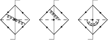
Figure 1: Diagrams for calculating the 𝒪⁡(αs)\mathcal{O}(\alpha_{s}) soft function. The solid lines represent Wilson lines in the light-like nn and n¯\bar{n} directions, the dashed lines represent Wilson lines in the vv direction, and the cut curly lines represent the cut gluon propagators.

Up to the NLO, the soft matrix elements accounting for soft gluon radiations from initial and final states can be obtained after calculating the Feynman diagrams shown in Fig. 1, and the soft function is given by

𝐒​(s​(1−z),μf)\displaystyle\mathbf{S}(\sqrt{s}(1-z),\mu_{f}) =\displaystyle= αs4​π[δ(1−z)(CD(−2L+4)+CF(2L2−π2))\displaystyle\frac{\alpha_{s}}{4\pi}\biggl[\delta(1-z)\bigl(C_{D}(-2L+4)+C_{F}(2L^{2}-\pi^{2})\bigr) (44)
+(−4CD+8CF(L−lnz))[11−z]++16CF[ln⁡(1−z)1−z]+].\displaystyle+\big(-4C_{D}+8C_{F}(L-\ln z)\big)\left[\frac{1}{1-z}\right]_{+}+16C_{F}\left[\frac{\ln(1-z)}{1-z}\right]_{+}\biggr].

It satisfies the RGE [30]

d​𝒲​(ω,μ)d​ln⁡μ\displaystyle\frac{d\ \mathcal{W}(\omega,\mu)}{d\ln\mu} =\displaystyle= −[4​Γcusp​(αs)​ln⁡ωμ+2​γW​(αs)]​𝒲​(ω,μ)\displaystyle-\left[4\Gamma_{\text{cusp}}(\alpha_{s})\ln\frac{\omega}{\mu}+2\gamma^{W}(\alpha_{s})\right]\mathcal{W}(\omega,\mu) (45)
−4Γcusp(αs)∫0ωdω′𝒲⁡(ω′,μ)−𝒲⁡(ω,μ)ω−ω′,\displaystyle-4\Gamma_{\text{cusp}}(\alpha_{s})\int_{0}^{\omega}d\omega^{\prime}\frac{\mathcal{W}(\omega^{\prime},\mu)-\mathcal{W}(\omega,\mu)}{\omega-\omega^{\prime}},

with

γW=2​γϕ+γH+γλ,\gamma^{W}=2\gamma^{\phi}+\gamma^{H}+\gamma^{\lambda}, (46)

where γϕ\gamma^{\phi} is the anomalous dimension of the PDF [43]. Its solution is [30]

𝒲(ω,μf)=exp[−4S(μs,μf)+2aγW(μs,μf)]s~(∂η,μs)1ω(ωμs)2​ηe−2​γE​ηΓ⁡(2​η),\mathcal{W}(\omega,\mu_{f})=exp\bigl[-4S(\mu_{s},\mu_{f})+2a_{\gamma^{W}}(\mu_{s},\mu_{f})\bigr]\tilde{s}(\partial_{\eta},\mu_{s})\frac{1}{\omega}\left(\frac{\omega}{\mu_{s}}\right)^{2\eta}\frac{e^{-2\gamma_{E}\eta}}{\Gamma(2\eta)}, (47)

with

η=2​aΓ​(μs,μf),\eta=2a_{\Gamma}(\mu_{s},\mu_{f}), (48)

where ∂η\partial_{\eta} is the derivative with respect to η\eta, and s~\tilde{s} is obtained by a Laplace transformation

s~​(L,μs)=∫0∞d​ω​e−s​ω​𝒲​(ω,μs)=1+αs4​π​[CD​(−2​L+4)+CF​(2​L2+43​π2)],\tilde{s}(L,\mu_{s})=\int_{0}^{\infty}d\omega e^{-s\omega}\mathcal{W}(\omega,\mu_{s})=1+\frac{\alpha_{s}}{4\pi}\biggl[C_{D}(-2L+4)+C_{F}\bigl(2L^{2}+\frac{4}{3}\pi^{2}\bigr)\biggr], (49)

with

s=1eγE​μs​eL/2.s=\frac{1}{e^{\gamma_{E}}\mu_{s}e^{L/2}}. (50)

Combining the above formulae, the RG-improved integral kernel is given by

C⁡(z,mϕ,μf)\displaystyle C(z,m_{\phi},\mu_{f}) =\displaystyle= λ2​(μλ)​|CH​(−mϕ2,μh)|2​U​(mϕ,μλ,μh,μs,μf)\displaystyle\lambda^{2}(\mu_{\lambda})|C_{H}(-m_{\phi}^{2},\mu_{h})|^{2}U(m_{\phi},\mu_{\lambda},\mu_{h},\mu_{s},\mu_{f}) (51)
⋅z−η(1−z)1−2​ηs~(lnmϕ2​(1−z)2μs2​z+∂η,μs)e−2​γE​ηΓ⁡(2​η),\displaystyle\cdot\frac{z^{-\eta}}{(1-z)^{1-2\eta}}\tilde{s}\left(\ln\frac{m_{\phi}^{2}(1-z)^{2}}{\mu_{s}^{2}z}+\partial_{\eta}\ ,\ \mu_{s}\right)\frac{e^{-2\gamma_{E}\eta}}{\Gamma(2\eta)},

with

U⁡(m,μλ,μh,μs,μf)\displaystyle U(m,\mu_{\lambda},\mu_{h},\mu_{s},\mu_{f}) =\displaystyle= (m2μh2)−2​aΓ​(μh,μs)\displaystyle\left(\frac{m^{2}}{\mu_{h}^{2}}\right)^{-2a_{\Gamma}(\mu_{h},\mu_{s})} (52)
×exp⁡[4​S​(μh,μs)+4​aγϕ​(μs,μf)−2​aγH​(μh,μs)−2​aγλ​(μλ,μs)].\displaystyle\times\exp\left[4S(\mu_{h},\mu_{s})+4a_{\gamma^{\phi}}(\mu_{s},\mu_{f})-2a_{\gamma^{H}}(\mu_{h},\mu_{s})-2a_{\gamma^{\lambda}}(\mu_{\lambda},\mu_{s})\right].
 RG-impr.PT  Log.approx  Accuracy∼αsn​Lk\sim\alpha_{s}^{n}L^{k}   Γcusp\Gamma_{\text{cusp}}   γH,γϕ,γλ\gamma^{H},\gamma^{\phi},\gamma^{\lambda}   CH,s~C_{H},\tilde{s}
- LL k=2​nk=2n   1-loop   tree-level   tree-level
LO NLL 2​n−1≤k≤2​n2n-1\leq k\leq 2n   2-loop   1-loop   tree-level
NLO NNLL 2​n−3≤k≤2​n2n-3\leq k\leq 2n   3-loop   2-loop   1-loop
Table 2: Schemes for resummation with different levels of accuracy.

For convenience, we list the counting scheme in Table 2, which shows corresponding requirements of different levels of accuracy [30]. Currently the two-loop γλ\gamma^{\lambda} is not available in the literature, so we just use the one-loop γλ\gamma^{\lambda}. The contribution of γλ\gamma^{\lambda} in the evolution function U⁡(m,μλ,μh,μs,μf)U(m,\mu_{\lambda},\mu_{h},\mu_{s},\mu_{f}) cancels out when μλ∼μh\mu_{\lambda}\sim\mu_{h}, so γλ\gamma^{\lambda} only affects the running of λ⁡(μλ)\lambda(\mu_{\lambda}), which gives a subordinate contribution. We then call our resummation an approximate next-to-next-to-leading logarithmic (NNLLapprox\text{NNLL}_{\text{approx}}), which is combined with the NLO results as follows:

d​σcombinedd​Y=d​σthreshd​Y|μλ,μh,μs,μf+(d​σfixed-orderd​Y|μf−d​σthreshd​Y|μλ=μh=μs=μf).\frac{d\sigma^{\text{combined}}}{dY}=\frac{d\sigma^{\text{thresh}}}{dY}\bigg|_{\mu_{\lambda},\mu_{h},\mu_{s},\mu_{f}}+\left(\frac{d\sigma^{\text{fixed-order}}}{dY}\bigg|_{\mu_{f}}-\frac{d\sigma^{\text{thresh}}}{dY}\bigg|_{\mu_{\lambda}=\mu_{h}=\mu_{s}=\mu_{f}}\right). (53)

V Numerical Discussion

In this section, we discuss the numerical results for threshold resummation effects in the single production of the color sextet (antitriplet) scalars at the LHC. Throughout our work the PDFsets MSTW2008lo and MSTW2008nlo [44, 45, 46] are used for LO, NLL and NLO, NNLLapprox{}_{\text{approx}}, respectively. If not explained specially, we will assume the coupling λ2​(MZ)=0.01​αs​(MZ)\lambda^{2}(M_{Z})=0.01\alpha_{s}(M_{Z}), and we choose the initial state quarks u​uuu for the sextet and u​dud for the antitriplet.

Refer to caption
Refer to caption
Refer to caption
Refer to caption
Figure 2: Comparison of the exact NLO results and the leading singular results. The long-dashed, dashed and solid lines correspond to LO, leading singular NLO and exact NLO results, respectively. The mass of the colored scalars is set to be 11 TeV in the rapidity distributions, and the center-of-mass energy of the colliding hadrons is set to be 1414 TeV.

The comparison between the leading singular results and the NLO results is shown in Fig. 2. We find that the leading singular terms give the dominant contribution, and the leading singular contribution of the sextet is smaller than the one of the antitriplet. The reason is that the terms associated with CDC_{D} give a negative contribution, and then a larger CDC_{D} of the sextet leads to smaller leading singular results.

Refer to caption
Refer to caption
Figure 3: The μh\mu_{h} dependence of the expansion coefficients c1c_{1} in the hard function.

Taking the perturbative convergence of CHC_{H} and s~\tilde{s} as the guiding principle, we can obtain the matching scales μh\mu_{h} and μs\mu_{s}. In Fig. 3 we show the μh\mu_{h} dependence of the expansion coefficient c1c_{1} defined in Eq.(36). We choose the hard scale μh0=0.535​mϕ\mu_{h}^{0}=0.535m_{\phi} for the sextet and μh0=1.63​mϕ\mu_{h}^{0}=1.63m_{\phi} for the antitriplet, respectively.

Refer to caption
Refer to caption
Figure 4: The μs\mu_{s} dependence of the soft function with different masses of the colored scalars.

The μs\mu_{s} dependence of the soft function is shown in Fig. 4. We fit the results and obtain the empirical functions:

sextet: μs0=mϕ​(1−τ)7+540​τ,\displaystyle\mu_{s}^{0}=\frac{m_{\phi}(1-\tau)}{\sqrt{7+540\tau}},
antitriplet: μs0=mϕ​(1−τ)4.6+362​τ.\displaystyle\mu_{s}^{0}=\frac{m_{\phi}(1-\tau)}{\sqrt{4.6+362\tau}}. (54)

It is required that μλ\mu_{\lambda} reflects the intensity of the interaction between the colored scalars and quarks, and μλ=μh\mu_{\lambda}=\mu_{h} is reasonable.

sextet
S\sqrt{S}=8 TeV S\sqrt{S}=14 TeV
 mϕm_{\phi}  LO  NLO  NLO+NNLLapprox{}_{\text{approx}}  LO  NLO  NLO+NNLLapprox{}_{\text{approx}}
 0.5 TeV  7.53  8.59  8.58  12.9  14.2  14.2
 1 TeV  0.768  0.916  0.918  1.46  1.68  1.68
 2 TeV  0.0416  0.0512  0.0529  0.137  0.165  0.165
antitriplet
S\sqrt{S}=8 TeV S\sqrt{S}=14 TeV
 mϕm_{\phi}  LO  NLO  NLO+NNLLapprox{}_{\text{approx}}  LO  NLO  NLO+NNLLapprox{}_{\text{approx}}
 0.5 TeV  4.85  6.13  6.21  9.17  11.1  11.2
 1 TeV  0.406  0.532  0.542  0.907  1.15  1.17
 2 TeV  0.0161  0.0215  0.0225  0.0686  0.899  0.916
Table 3: Numerical results of the total cross section (unit: pb).

In Table 3, we list the typical results of total cross sections, which compare NLO+NNLLapprox{}_{\text{approx}} with LO and NLO results. From Table 3, we can see that the resummation effects increase the NLO total cross section by about 2%2\% and 0.2%0.2\% for 1 TeV antitriplet and sextet, respectively, and 5%5\% and 3%3\% for 2 TeV antitriplet and sextet, respectively, at the 8 TeV LHC. And the resummation effects at the 14 TeV LHC are smaller than the ones at the 8 TeV LHC.

Refer to caption
Refer to caption
Figure 5: The fixed-order and RG-improved cross section predictions including perturbative uncertainty bands due to variations of scale μf\mu_{f}.

In Fig. 5, we show the dependence of the total cross section on the scalar masses including perturbative uncertainty bands due to variation of scale μf\mu_{f} at the 8 TeV LHC. We find that the threshold resummation reduces the scale dependence of the total cross section. The scenario at the 14 TeV LHC is very similar, so we do not present it in the figures.

Refer to caption
Refer to caption
Refer to caption
Refer to caption
Figure 6: The μh\mu_{h} and μs\mu_{s} dependence of the resummed total cross sections. The solid and dashed lines represent μh\mu_{h} and μs\mu_{s} dependence, respectively. We set the scalar mass to be 1 TeV.

Fig. 6 shows the dependence of the resummed total cross section on μh\mu_{h} and μs\mu_{s}. The scales are varied over the ranges μh0/2<μh<2​μh0\mu_{h}^{0}/2<\mu_{h}<2\mu_{h}^{0} and μs0/2<μs<2​μs0\mu_{s}^{0}/2<\mu_{s}<2\mu_{s}^{0}, respectively. From Fig. 6, we can see that the μh\mu_{h} dependence of the sextet is more sensitive than the antitriplet.

Refer to caption
Refer to caption
Refer to caption
Refer to caption
Figure 7: The comparison of the rapidity distributions between the combined resummation results and the fixed-order results for sextet and antitriplet. The scalar mass is set to be 1 TeV. The lighter bands stand for LO and NLL, while the darker represent NLO and NNLLapprox{}_{\text{approx}}.

In Fig. 7, we present the rapidity distributions, which compare the resummation results combined in Eq.(53) with the fixed-order results. The scale μf\mu_{f} is varied over the range mϕ/2<μf<2​mϕm_{\phi}/2<\mu_{f}<2m_{\phi}. We find that the shapes of the rapidity distribution of the resummation change slightly over the fixed-order results, and resummation reduces the scale dependence, except the NNLLapprox{}_{\text{approx}} results of the sextet cases. This is caused by the large color factor for the sextet (CD=10/3C_{D}=10/3 for the sextet, CD=4/3C_{D}=4/3 for the antitriplet). The terms containing a large color factor CDC_{D}, which is associated with the scale dependence of λ\lambda and αs\alpha_{s}, will enlarge the scale dependence of the NNLLapprox{}_{\text{approx}} results of sextet.

Refer to caption
Refer to caption
Refer to caption
Refer to caption
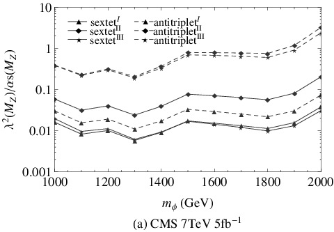
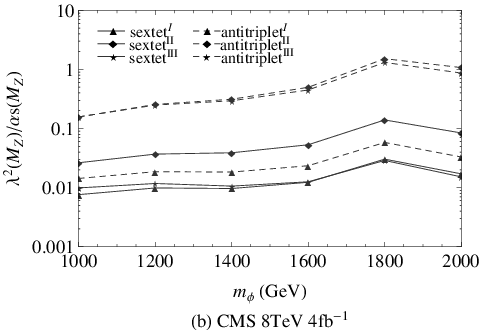
Figure 8: Constraint on the couplings λ\lambda of the colored scalars with different electronic charges.

Finally, we use recent dijet data at the LHC to give constraints on the couplings λ\lambda. The CMS collaboration published the results of dijet production based on 5 fb-1 of 7 TeV data and 4 fb-1 of 8 TeV data [21, 22, 23], and the ATLAS collaboration based on 4.8 fb-1 of 7 TeV data and 13 fb-1 of 8 TeV data [47, 48]. Using the narrow-width-approximation [49], the total cross section can be written as

σ\displaystyle\sigma =\displaystyle= (2​π)72​S​∫qm​i​n2qm​a​x2d​q2​∫d​ϕp​d​ϕd​|ℳp​(q2)|2​[(q2−m2)2+(m​Γ)2]−1​|ℳd​(q2)|2\displaystyle\frac{(2\pi)^{7}}{2S}\int_{q_{min}^{2}}^{q_{max}^{2}}dq^{2}\int d\phi_{p}\ d\phi_{d}\big|\mathcal{M}_{p}(q^{2})\big|^{2}\big[(q^{2}-m^{2})^{2}+(m\Gamma)^{2}\big]^{-1}\big|\mathcal{M}_{d}(q^{2})\big|^{2} (55)
=\displaystyle= (2​π)84​S​m​Γ​∫d​ϕp​|ℳp​(q2)|2​∫d​ϕd​|ℳd​(q2)|2.\displaystyle\frac{(2\pi)^{8}}{4Sm\Gamma}\int d\phi_{p}\big|\mathcal{M}_{p}(q^{2})\big|^{2}\int d\phi_{d}\big|\mathcal{M}_{d}(q^{2})\big|^{2}.

After fitting the dijet data, we can give the constraints on the couplings. Since there is no direct theoretical requirement on the couplings between the colored scalars and different quarks, we use a common value for the coupling λ\lambda here. The colored scalars with different electronic charges couple to different quarks, and then they receive different constraints. In Fig. 8, we show the results of the constraints on the couplings. The most stringent constraint on s​e​x​t​e​tIsextet^{I} is λ2​(MZ)≥0.006​αs​(MZ)\lambda^{2}(M_{Z})\geq 0.006\alpha_{s}(M_{Z}), and similarly the other constraints are 0.024αs​(MZ)\alpha_{s}(M_{Z}), 0.006αs​(MZ)\alpha_{s}(M_{Z}), 0.011αs​(MZ)\alpha_{s}(M_{Z}), 0.16αs​(MZ)\alpha_{s}(M_{Z}) and 0.16αs​(MZ)\alpha_{s}(M_{Z}) for s​e​x​t​e​tI​Isextet^{II}, s​e​x​t​e​tI​I​Isextet^{III}, a​n​t​i​t​r​i​p​l​e​tIantitriplet^{I}, a​n​t​i​t​r​i​p​l​e​tI​Iantitriplet^{II} and a​n​t​i​t​r​i​p​l​e​tI​I​Iantitriplet^{III}, respectively.

VI Conclusion

We have studied the threshold resummation effects in the single production of the color sextet (antitriplet) scalars at the LHC with the soft-collinear effective theory. We find that the resummation effects increase the NLO total cross section by about 2%2\% and 0.2%0.2\% for 1 TeV color antitriplet and sextet scalar, respectively, and 5%5\% and 3%3\% for 2 TeV color antitriplet and sextet scalar, respectively, at the 8 TeV LHC. The resummation effects improve the scale dependence of the cross section and the rapidity distribution generally. But in the case of the rapidity distribution of the color sextet scalar, the scale dependence is not improved because of the large color factor CDC_{D} (CD=10/3C_{D}=10/3 for the sextet, CD=4/3C_{D}=4/3 for the antitriplet) enlarging the scale dependence. Besides, we use recent dijet data from the LHC to give constraints on the couplings. For different colored scalars with different electronic charges, the most stringent constraints of λ2​(MZ)\lambda^{2}(M_{Z}) range from 0.006αs​(MZ)\alpha_{s}(M_{Z}) to 0.16αs​(MZ)\alpha_{s}(M_{Z}).

Acknowledgements.
We would like to thank Hua Xing Zhu, Jian Wang and Qing Hong Cao for useful discussions. This work was supported in part by the National Natural Science Foundation of China, under Grants No. 11375013 and No. 11135003.

Appendix A Relevant Feynman Diagrams

Relevant Feynman diagrams for the production of the colored scalar are shown in Fig. 9.

Refer to caption
Figure 9: Relevant Feynman diagrams for the production of the colored scalar.

References

  • [1] A. Mete, ATL-PHYS-PROC-2012-201, ATL-COM-PHYS-2012-1365 (2012).
  • [2] O. Vickey Boeriu, ATL-PHYS-PROC-2012-051, ATL-COM-PHYS-2012-313 (2012).
  • [3] T. Lari, ATL-PHYS-PROC-2011-150, ATL-COM-PHYS-2011-1340 (2011).
  • [4] ATLAS, https://twiki.cern.ch/twiki/bin/view/AtlasPublic/CombinedSummaryPlots (2012).
  • [5] CMS, https://twiki.cern.ch/twiki/bin/view/CMSPublic/PhysicsResults (2012).
  • [6] J. C. Pati and A. Salam, Phys.Rev. D10, 275 (1974).
  • [7] R. N. Mohapatra and R. Marshak, Phys.Rev.Lett. 44, 1316 (1980).
  • [8] P. Fileviez Perez, Phys.Lett. B654, 189 (2007), eprint hep-ph/0702287.
  • [9] R. Barbier, C. Berat, M. Besancon, M. Chemtob, A. Deandrea, et al., Phys.Rept. 420, 1 (2005), eprint hep-ph/0406039.
  • [10] R. Mohapatra, N. Okada, and H.-B. Yu, Phys.Rev. D77, 011701 (2008), eprint 0709.1486.
  • [11] Z. Chacko and R. Mohapatra, Phys.Rev. D59, 055004 (1999), eprint hep-ph/9802388.
  • [12] T. Han, I. Lewis, and T. McElmurry, JHEP 1001, 123 (2010a), eprint 0909.2666.
  • [13] E. Del Nobile, R. Franceschini, D. Pappadopulo, and A. Strumia, Nucl.Phys. B826, 217 (2010), eprint 0908.1567.
  • [14] C.-H. Chen, Phys.Lett. B680, 133 (2009), eprint 0902.2620.
  • [15] C.-R. Chen, W. Klemm, V. Rentala, and K. Wang, Phys.Rev. D79, 054002 (2009), eprint 0811.2105.
  • [16] I. Gogoladze, Y. Mimura, N. Okada, and Q. Shafi, Phys.Lett. B686, 233 (2010), eprint 1001.5260.
  • [17] E. L. Berger, Q.-H. Cao, C.-R. Chen, G. Shaughnessy, and H. Zhang, Phys.Rev.Lett. 105, 181802 (2010), eprint 1005.2622.
  • [18] T. Han, I. Lewis, and Z. Liu, JHEP 1012, 085 (2010b), eprint 1010.4309.
  • [19] P. Richardson and D. Winn, Eur.Phys.J. C72, 1862 (2012), eprint 1108.6154.
  • [20] D. Karabacak, S. Nandi, and S. K. Rai, Phys.Rev. D85, 075011 (2012), eprint 1201.2917.
  • [21] S. Chatrchyan et al. (CMS Collaboration), JHEP 1301, 013 (2013a), eprint 1210.2387.
  • [22] S. Chatrchyan et al. (CMS Collaboration) (2013b), eprint 1302.4794.
  • [23] Tech. Rep. CMS-PAS-EXO-12-059, CERN, Geneva (2013).
  • [24] J. L. Hewett and T. G. Rizzo, Phys.Rept. 183, 193 (1989).
  • [25] C. W. Bauer, S. Fleming, D. Pirjol, and I. W. Stewart, Phys.Rev. D63, 114020 (2001), eprint hep-ph/0011336.
  • [26] C. W. Bauer, D. Pirjol, and I. W. Stewart, Phys.Rev. D65, 054022 (2002a), eprint hep-ph/0109045.
  • [27] M. Beneke, A. Chapovsky, M. Diehl, and T. Feldmann, Nucl.Phys. B643, 431 (2002), eprint hep-ph/0206152.
  • [28] C. W. Bauer, S. Fleming, and M. E. Luke, Phys.Rev. D63, 014006 (2000), eprint hep-ph/0005275.
  • [29] C. W. Bauer, S. Fleming, D. Pirjol, I. Z. Rothstein, and I. W. Stewart, Phys.Rev. D66, 014017 (2002b), eprint hep-ph/0202088.
  • [30] T. Becher, M. Neubert, and G. Xu, JHEP 0807, 030 (2008), eprint 0710.0680.
  • [31] C. Anastasiou, L. J. Dixon, K. Melnikov, and F. Petriello, Phys.Rev. D69, 094008 (2004), eprint hep-ph/0312266.
  • [32] H. Baer, J. Ohnemus, and J. Owens, Phys.Lett. B234, 127 (1990).
  • [33] B. Harris and J. Owens, Phys.Rev. D65, 094032 (2002), eprint hep-ph/0102128.
  • [34] J. C. Collins, D. E. Soper, and G. F. Sterman, Nucl.Phys. B261, 104 (1985).
  • [35] G. T. Bodwin, Phys.Rev. D31, 2616 (1985).
  • [36] G. Altarelli and G. Parisi, Nucl.Phys. B126, 298 (1977).
  • [37] R. J. Hill and M. Neubert, Nucl.Phys. B657, 229 (2003), eprint hep-ph/0211018.
  • [38] T. Becher, R. J. Hill, and M. Neubert, Phys.Rev. D69, 054017 (2004), eprint hep-ph/0308122.
  • [39] J. C. Collins and D. E. Soper, Nucl.Phys. B194, 445 (1982).
  • [40] V. Ahrens, T. Becher, M. Neubert, and L. L. Yang, Eur.Phys.J. C62, 333 (2009), eprint 0809.4283.
  • [41] T. Gehrmann, T. Huber, and D. Maitre, Phys.Lett. B622, 295 (2005), eprint hep-ph/0507061.
  • [42] T. Becher and M. Neubert, Phys.Rev. D79, 125004 (2009), eprint 0904.1021.
  • [43] S. Moch, J. Vermaseren, and A. Vogt, Nucl.Phys. B688, 101 (2004), eprint hep-ph/0403192.
  • [44] A. Martin, W. Stirling, R. Thorne, and G. Watt, Eur.Phys.J. C63, 189 (2009a), eprint 0901.0002.
  • [45] A. Martin, W. Stirling, R. Thorne, and G. Watt, Eur.Phys.J. C64, 653 (2009b), eprint 0905.3531.
  • [46] A. Martin, W. Stirling, R. Thorne, and G. Watt, Eur.Phys.J. C70, 51 (2010), eprint 1007.2624.
  • [47] G. Aad et al. (ATLAS Collaboration), JHEP 1301, 029 (2013), eprint 1210.1718.
  • [48] Tech. Rep. ATLAS-CONF-2012-148, CERN, Geneva (2012).
  • [49] N. Kauer, Phys.Lett. B649, 413 (2007), eprint hep-ph/0703077.