跳到论文正文
W Papers独立论文阅读器 arXiv:1305.5056 论文正文 计算阅读时间 · 0%
引用这篇论文根据当前论文元数据生成,正式投稿前建议核对。


License: CC BY-NC-SA 3.0
arXiv:1305.5056v2 [quant-ph] 05 Dec 2014

Comparison of Electromagnetically Induced Transparency in lambda, cascade and vee three-level systems

Surajit Sena∗    Tushar Kanti Deya†    Mihir Ranjan Natha‡ and Gautam Gangopadhyayb¶
aPhysics Department
††thanks: $ˆ∗$ ssen55@yahoo.com,   $ˆ†$ tkdey54@gmail.com,   $ˆ‡$ mrnath_95@rediffmail.com,   $ˆ¶$ gautam@bose.res.in
   Guru Charan College    Silchar - 788004    India
bS N Bose National Centre for Basic Sciences
   JD Block    Sector III   
Salt Lake City
   Kolkata 700098    India
Abstract

We discuss the Electromagnetically Induced Transparency (EIT) in lambda, cascade and vee type three-level systems where the Hamiltonian and the Lindblad term of each configuration are expressed in the S​U​(3)SU(3) representation. At steady state, the Optical Bloch Equations of each configuration are solved to obtain the dispersion and absorption profiles of the probe field along with their group velocities. When the EIT condition is achieved at resonance, the population oscillation shows which of the bare states are contributing to form the dark state. Our study reveals that the dark state for the lambda and cascade system effectively coincides with the lowest bare state of that system, while for the vee system, it is a maximally superposed state of the middle and upper bare states.

keywords
S​U​(3)SU(3) group; Electromagnetically Induced Transparency (EIT); Three-level system

Abstract

1 Introduction

It is well known that the physical properties of the bulk material, namely, absorption coefficient, refractive index, conductivity etc can be maneuvered by the passage of light through it. In this respect, the quantum coherence plays a key role where their optical properties can be selectively modified by a number of effect, e.g., coherent population trapping (CPT) [1, 2], lasing without inversion (LWI) [3, 4], Electromagnetically Induced Transparency (EIT) [5, 6, 7, 8, 9, 10], high refractive index without absorption  [11, 12], giant Kerr effect [13] etc. Out of them, the EIT is possibly the most successful coherent phenomenon by which the transparency of a medium can be achieved by the simultaneous action of two laser sources while satisfying some delicate conditions of the quantum interference  [6, 9, 14]. Since its discovery in 1989 [15] which is followed by the experimental observation in 1990  [5], the study of EIT has become a promising area of research because of its amazing ability of ceasing the group velocity of light pulse when the number density of atom is very high [16, 17, 18].

The manipulation of the optical property of a medium by EIT requires a clear understanding of the level structure of atoms with which the medium is composed of. In a nutshell, this phenomenon can be illustrated as follows: Two beams of coherent light, one with strong driving capability (called control or pump field) in comparison to the weaker one (called probe field), are allowed to incident on a medium which consists of three-level system. Because of an intricate role of quantum coherence at the resonant pump-probe combination, the medium, which is initially opaque to the probe field, becomes almost transparent. At steady state for the resonant probe pulse, the refractive index becomes unity and the coefficient of absorption is dropped to zero by opening a narrow transparency window called Autler-Towns splitting. More precisely, the steep and positive slope of the refractive index curve leads to the significant reduction of the group velocity of light  [19, 17, 16]. Using the dressed atom formalism, the physics behind the transparency is explained by the trapping of all atoms into the dark state, the state which is formed due to the superposition of two mutually uncoupled bare states of the three-level system [20].

It is now widely accepted that the three-level systems, which exhibits this intriguing optical property, can be classified into the lambda, cascade and vee type of systems and they are intrinsically different from one another [21]. In literature, the theoretical study of the EIT phenomenon is extensively made primarily with the lambda system than in comparison to its other two counterparts [22, 23, 24]. There we have noted several contradictory remarks. For example, Ref. [9, 23] argue that the EIT can be observed in cascade system which contravenes with remarks of Ref. [10] that advocates the nonobservance of the EIT for the cascade and vee systems because of the absence of the meta-stable dark state. Recently, the possibility of distinct coherent process for the vee system contrast to the lambda system is hinted in some studies [24]. These conflicting comments on different models is possibly due to the inconspicuous and incomplete presentation of the EIT which lacks rigorous mathematical treatment of all three-level systems in equal footing. The purpose of the present work is to fill up this gap and to make a systematic study vis-a`\grave{a}-vis careful scrutiny of all three configurations to look for the underlying physical mechanism in terms of their dark state [20].

Apart from that, there is another reason for the systematic study of EIT which is known to be associated with two concomitant phenomena, namely, the coherent population trapping (CPT) and the formation of the dark state. The CPT is a standard feature of all three-level systems where whole population is being trapped in the non-evolving dark state. Although, the existence of such state is understood by noting the vanishing eigen value of the Hamiltonian of a given three-level system, but whether its formal structure remains unaltered in presence of the dissipation, is an intricate issue and, therefore, needs a closer inspection.

Based on the SU(3) representation of the three-level system, recently, we have developed the model Hamiltonians of the lambda, vee and cascade systems and have solved them exactly both for the semiclassical and the quantized bichromatic fields [21]. These models form the basis of developing a rigorous and systematic treatment of EIT presented in this paper. To introduce damping using Lindlad formalism, we have used the shift operators of the SU(3) representation rather than invoking them phenomenologically. In addition, to understand the level where the atoms are being trapped, we have studied the population oscillation of each model as the function of probe-field detuning frequency. Our study reveals the constitutive bare states of the dark state for all three configurations.

The remainder of the paper is organized as follows: In Section 2 we introduce the master equation of the lambda, vee and cascade systems where the model Hamiltonians and the Lindblad terms are written using the shift operators of the S​U​(3)SU(3) representation. The requisite theory to find the dispersion and absorption profiles of the probe field along with its group velocity is also outlined. Section 3 illustrates the steady state solution of the Optical Bloch Equations of the lambda, vee and cascade systems at resonant frequency of the probe field necessary to calculate the refractive index and the coefficient of absorption of the medium. Section 4 gives the numerical solution of the three systems and discuss the scenario of EIT by analyzing the population distribution in different states. Finally we summarize the main results of the paper and discuss the outlook.

2 The models

The master equation for the three-level systems with Lindblad term is given by (A=Λ,V,ΞA=\Lambda,\,V,\,\Xi),

d​ρAd​t=iℏ​[ρA,HA]+𝔏DA,\frac{{d\rho^{A}}}{{dt}}=\frac{i}{\hbar}\left[{\rho^{A},H^{A}}\right]+\mathfrak{L}_{D}^{A}, (1)

where the density matrix is defined by,

ρA=[ρ33ρ32ρ31ρ23ρ22ρ21ρ13ρ12ρ11],\rho^{A}=\left[{\begin{array}[]{*{20}c}{\rho_{33}}&{\rho_{32}}&{\rho_{31}}\\ {\rho_{23}}&{\rho_{22}}&{\rho_{21}}\\ {\rho_{13}}&{\rho_{12}}&{\rho_{11}}\\ \end{array}}\right], (2)

with the basis states, |1>=(0,0,1)T|1>=(0,0,1)^{T}, |2>=(0,1,0)T|2>=(0,1,0)^{T} and |3>=(1,0,0)T|3>=(1,0,0)^{T} being the lower, middle and upper states, respectively. The lambda, cascade and vee configurations of the three-level system are shown in Fig.1 and their levels follow same energy hierarchy condition, namely, E1<E2<E3E_{1}<E_{2}<E_{3}. In Eq.(1), the Hamiltonian of the semiclassical three-level system in the rotating wave approximation (RWA) in the S​U​(3)SU(3) representation is given by  [21],

HΛ=ω1​V3+ω2​T3+g13​V+​exp⁡(−i​ω13​t)+g23​T+​exp⁡(−i​ω23​t)+h.c.,\displaystyle H^{\Lambda}=\omega_{1}V_{3}+\omega_{2}T_{3}+g_{13}V_{+}\exp(-i\omega_{13}t)+g_{23}T_{+}\exp(-i\omega_{23}t)+h.c., (3a)
for the lambda system,
HΞ=ω1​U3+ω2​T3+g12​U+​exp⁡(−i​ω12​t)+g23​T+​exp⁡(−i​ω23​t)+h.c.,\displaystyle H^{\Xi}=\omega_{1}U_{3}+\omega_{2}T_{3}+g_{12}U_{+}\exp(-i\omega_{12}t)+g_{23}T_{+}\exp(-i\omega_{23}t)+h.c., (3b)
for the cascade system,
HV=ω1​V3+ω2​U3+g13​V+​exp⁡(−i​ω13​t)+g12​U+​exp⁡(−i​ω12​t)+h.c.,\displaystyle H^{V}=\omega_{1}V_{3}+\omega_{2}U_{3}+g_{13}V_{+}\exp(-i\omega_{13}t)+g_{12}U_{+}\exp(-i\omega_{12}t)+h.c., (3c)

for the vee system, respectively. Here, Ta,Va,UaT_{a},V_{a},U_{a} (a=+,−,3a=+,-,3) be the shift operators of S​U​(3)SU(3) representation [25], gi​jg_{ij} (i,j=1,2,3i,j=1,2,3) be the coupling parameters and ωi​j\omega_{ij} be the frequencies of the applied bi-chromatic laser fields, respectively. The S​U​(3)SU(3) Lindblad terms of three configurations appearing in Eq.(1) are given by,

𝔏DΛ=Γ31Λ​(V+​V−​ρΛ−2​V−​ρΛ​V++ρΛ​V+​V−)+Γ32Λ​(T+​T−​ρΛ−2​T−​ρΛ​T++ρΛ​T+​T−),\displaystyle\mathfrak{L}_{D}^{\Lambda}=\Gamma_{31}^{\Lambda}(V_{+}V_{-}\rho^{\Lambda}-2V_{-}\rho^{\Lambda}V_{+}+\rho^{\Lambda}V_{+}V_{-})+\Gamma_{32}^{\Lambda}(T_{+}T_{-}\rho^{\Lambda}-2T_{-}\rho^{\Lambda}T_{+}+\rho^{\Lambda}T_{+}T_{-}), (4a)
for the lambda system,
𝔏DΞ\displaystyle\mathfrak{L}_{D}^{\Xi} =\displaystyle= Γ32Ξ​(T+​T−​ρΞ−2​T−​ρΞ​T++ρΞ​T+​T−)+Γ21Ξ​(U+​U−​ρΞ−2​U−​ρΞ​U++ρΞ​U+​U−),\displaystyle\Gamma_{32}^{\Xi}(T_{+}T_{-}\rho^{\Xi}-2T_{-}\rho^{\Xi}T_{+}+\rho^{\Xi}T_{+}T_{-})+\Gamma_{21}^{\Xi}(U_{+}U_{-}\rho^{\Xi}-2U_{-}\rho^{\Xi}U_{+}+\rho^{\Xi}U_{+}U_{-}), (4b)
for the cascade systems,
𝔏DV\displaystyle\mathfrak{L}_{D}^{V} =\displaystyle= Γ31V​(V+​V−​ρV−2​V−​ρV​V++ρV​V+​V−)+Γ21V​(U+​U−​ρV−2​U−​ρV​U++ρV​U+​U−),\displaystyle\Gamma_{31}^{V}(V_{+}V_{-}\rho^{V}-2V_{-}\rho^{V}V_{+}+\rho^{V}V_{+}V_{-})+\Gamma_{21}^{V}(U_{+}U_{-}\rho^{V}-2U_{-}\rho^{V}U_{+}+\rho^{V}U_{+}U_{-}), (4c)

for the vee system, respectively. It is evident from Fig.1 that for the lambda system, the spontaneous decay from lower to higher level ( i.e., 1 to 3 and 2 to 3) is not permitted and therefore, Γ13Λ=Γ23Λ=0\Gamma_{13}^{\Lambda}=\Gamma_{23}^{\Lambda}=0. For the same reason, we have Γ12Ξ=Γ13Ξ=0\Gamma_{12}^{\Xi}=\Gamma_{13}^{\Xi}=0 for the cascade system and Γ13V=Γ12V=0\Gamma_{13}^{V}=\Gamma_{12}^{V}=0 for the vee system, respectively. Thus, as shown in Fig.1, the control and probe fields correspond 2↔32\leftrightarrow 3 and 1↔31\leftrightarrow 3 dipole transition for the lambda system, 1↔21\leftrightarrow 2 and 1↔31\leftrightarrow 3 transition for the vee system and 2↔32\leftrightarrow 3 and 1↔21\leftrightarrow 2 transition for the cascade system, respectively. The generic detuning condition in the S​U​(3)SU(3) representation is given by Δk​lA=(m​ω1+n​ω2−ωk​l)\Delta^{A}_{kl}=(m\omega_{1}+n\omega_{2}-\omega_{kl}), where m,n∈ℤm,n\in\mathbb{Z} [21].

To understand the dispersion and absorption profiles of the medium at resonance, we need to evaluate the steady state density matrix ρsA\rho^{A}_{s} by solving the equation ρ˙A​(t)=0\dot{\rho}^{A}(t)=0 from Eq.(1) formally known as Optical Bloch Equation (OBE). Given with the steady state density matrix ρsA\rho^{A}_{s}, it is convenient to express the real and imaginary parts of the susceptibility in terms of Bloch vectors which gives the refractive index and coefficient of absorption of the probe field,

nA​(Δi​jA)=1+N0​μi​j22​ϵ0​ℏ​T​r​[ρsA​λa],\displaystyle n^{A}(\Delta^{A}_{ij})=1+\frac{N_{0}\mu_{ij}^{2}}{2\epsilon_{0}\hbar}Tr[\rho^{A}_{s}\lambda_{a}], (5)
αA​(Δi​jA)=N0​μi​j22​ϵ0​ℏ​T​r​[ρsA​λa¯],\displaystyle\alpha^{A}(\Delta^{A}_{ij})=\frac{N_{0}\mu_{ij}^{2}}{2\epsilon_{0}\hbar}Tr[\rho^{A}_{s}\lambda_{\bar{a}}], (6)

respectively, where N0N_{0} be the number of three-level configuration in the sample, μi​j\mu_{ij} be the dipole moment of i↔ji\leftrightarrow j transition and ϵ0\epsilon_{0} be the permittivity of free space, respectively. In Eqs.(5) and (6), the Gellmann matrix λa\lambda_{a} is judiciously chosen so that it projects requisite terms from the density matrix which contributes in i↔ji\leftrightarrow j dipole transition.

Δ 32 Λ
| 3 >
| 3 >
Figure 1: Lambda, Cascade and Vee type three-level configurations with the energy levels arranged as E3>E2>E1E_{3}>E_{2}>E_{1}. The detuning from the applied field are Δ23Λ=ω1+2​ω2−ω23\Delta^{\Lambda}_{23}=\omega_{1}+2\omega_{2}-\omega_{23} and Δ13Λ=2​ω1+ω2−ω13\Delta^{\Lambda}_{13}=2\omega_{1}+\omega_{2}-\omega_{13} for the lambda system, Δ23Ξ=−ω1+2​ω2−ω23\Delta^{\Xi}_{23}=-\omega_{1}+2\omega_{2}-\omega_{23} and Δ12Ξ=2​ω1−ω2−ω12\Delta^{\Xi}_{12}=2\omega_{1}-\omega_{2}-\omega_{12} for the cascade system and Δ12V=2​ω1+ω2−ω12\Delta^{V}_{12}=2\omega_{1}+\omega_{2}-\omega_{12} and Δ13V=ω1+2​ω2−ω13\Delta^{V}_{13}=\omega_{1}+2\omega_{2}-\omega_{13} for the vee system, respectively  [21].

Finally, the group velocity of probe field through the medium is calculated using vg=c/ngv_{g}=c/n_{g}, where the group refractive index for the probe field of frequency ωi​j\omega_{ij} is given by,

ngA​(Δi​jA)\displaystyle n^{A}_{g}(\Delta^{A}_{ij}) =\displaystyle= nA​(Δi​jA)+ωi​j​d​nA​(Δi​jA)d​ωi​j\displaystyle n^{A}(\Delta^{A}_{ij})+\omega_{ij}\frac{dn^{A}(\Delta^{A}_{ij})}{d\omega_{ij}} (7)
=\displaystyle= nA​(Δi​jA)+ωi​j​∂nA​(Δi​jA)∂|Δi​jA|⋅∂|Δi​jA|∂ωi​j,\displaystyle n^{A}(\Delta^{A}_{ij})+\omega_{ij}\frac{\partial n^{A}(\Delta^{A}_{ij})}{\partial\big|\Delta^{A}_{ij}\big|}\cdot\frac{\partial\big|\Delta^{A}_{ij}\big|}{\partial\omega_{ij}},

By noting the fact that, d​|Δk​lA|d​ωk​l=1\frac{d\big|\Delta^{A}_{kl}\big|}{d\omega_{kl}}=1, the group velocity is simplified to,

vgA​(Δi​jA)=c/(1+N0​μi​j2​ωi​j2​ϵ0​ℏ​∂(T​r​[ρsA​λa])∂Δi​jA).v^{A}_{g}(\Delta^{A}_{ij})=c/\big(1+\frac{N_{0}\mu_{ij}^{2}\omega_{ij}}{2\epsilon_{0}\hbar}\frac{\partial(Tr[\rho_{s}^{A}\lambda_{a}])}{\partial\Delta^{A}_{ij}}\big). (8)

The positive slope of the dispersion curve near resonance ensures the reduction of the group velocity which is different for different three-level systems. In the subsequent Sections we proceed to solve the master equations with the aforesaid S​U​(3)SU(3) Lindblad terms to find steady state density matrix of all three configurations and explore the EIT effect and its associated phenomena, e.g., the group velocity reduction, coherent trapping, dark state etc.

3 EIT in three-level systems

3.1 Lambda system

To obtain the Optical Bloch Equation of the lambda system we consider the master equation with the Hamiltonian given by Eq.(3a) and the corresponding Lindblad term in Eq.(4a). The following substitutions eliminate the phase terms appearing in the density matrix equations,

ρ11Λ\displaystyle\rho_{11}^{\Lambda} →\displaystyle\rightarrow ρ~11Λ=ρ11Λ,\displaystyle\tilde{\rho}_{11}^{\Lambda}=\rho_{11}^{\Lambda},
ρ22Λ\displaystyle\rho_{22}^{\Lambda} →\displaystyle\rightarrow ρ~22Λ=ρ22Λ,\displaystyle\tilde{\rho}_{22}^{\Lambda}=\rho_{22}^{\Lambda},
ρ33Λ\displaystyle\rho_{33}^{\Lambda} →\displaystyle\rightarrow ρ~33Λ=ρ33Λ,\displaystyle\tilde{\rho}_{33}^{\Lambda}=\rho_{33}^{\Lambda},
ρ13Λ\displaystyle\rho_{13}^{\Lambda} →\displaystyle\rightarrow ρ~13Λ=ρ~31Λ∗=ei​ω13​tρ13Λ,\displaystyle\tilde{\rho}_{13}^{\Lambda}=\tilde{\rho}_{31}^{\Lambda*}=e^{i\omega_{13}t}\rho_{13}^{\Lambda},
ρ12Λ\displaystyle\rho_{12}^{\Lambda} →\displaystyle\rightarrow ρ~12Λ=ρ~21Λ∗=ei⁡(ω13−ω23)​tρ12Λ,\displaystyle\tilde{\rho}_{12}^{\Lambda}=\tilde{\rho}_{21}^{\Lambda*}=e^{i(\omega_{13}-\omega_{23})t}\rho_{12}^{\Lambda},
ρ23Λ\displaystyle\rho_{23}^{\Lambda} →\displaystyle\rightarrow ρ~23Λ=ρ~32Λ∗=ei​ω23​tρ23Λ.\displaystyle\tilde{\rho}_{23}^{\Lambda}=\tilde{\rho}_{32}^{\Lambda*}=e^{i\omega_{23}t}\rho_{23}^{\Lambda}. (9)

Using the detuning conditions to be, Δ23Λ=ω1+2​ω2−ω23\Delta_{23}^{\Lambda}=\omega_{1}+2\omega_{2}-\omega_{23} and Δ13Λ=2​ω1+ω2−ω13\Delta^{\Lambda}_{13}=2\omega_{1}+\omega_{2}-\omega_{13}, respectively, we obtain the following OBE (here we drop the tilde sign),

ρ˙11Λ\displaystyle\dot{\rho}_{11}^{\Lambda} =\displaystyle= i​g13​(ρ13Λ−ρ31Λ)+2​Γ31Λ​ρ33Λ\displaystyle ig_{13}(\rho_{13}^{\Lambda}-\rho_{31}^{\Lambda})+2\Gamma_{31}^{\Lambda}\rho_{33}^{\Lambda}
ρ˙22Λ\displaystyle\dot{\rho}_{22}^{\Lambda} =\displaystyle= i​g23​(ρ23Λ−ρ32Λ)+2​Γ32Λ​ρ33Λ\displaystyle ig_{23}(\rho_{23}^{\Lambda}-\rho_{32}^{\Lambda})+2\Gamma_{32}^{\Lambda}\rho_{33}^{\Lambda}
ρ˙33Λ\displaystyle\dot{\rho}_{33}^{\Lambda} =\displaystyle= −i​g13​(ρ13Λ−ρ31Λ)−i​g23​(ρ23Λ−ρ32Λ)−2​(Γ31Λ+Γ32Λ)​ρ33Λ\displaystyle-ig_{13}(\rho_{13}^{\Lambda}-\rho_{31}^{\Lambda})-ig_{23}(\rho_{23}^{\Lambda}-\rho_{32}^{\Lambda})-2(\Gamma_{31}^{\Lambda}+\Gamma_{32}^{\Lambda})\rho_{33}^{\Lambda}
ρ˙12Λ\displaystyle\dot{\rho}_{12}^{\Lambda} =\displaystyle= ρ˙21Λ∗=i(Δ13Λρ12Λ−Δ23Λρ12Λ+g23ρ13Λ−g13ρ32Λ)\displaystyle\dot{\rho}_{21}^{\Lambda*}=i(\Delta_{13}^{\Lambda}\rho_{12}^{\Lambda}-\Delta_{23}^{\Lambda}\rho_{12}^{\Lambda}+g_{23}\rho_{13}^{\Lambda}-g_{13}\rho_{32}^{\Lambda})
ρ˙13Λ\displaystyle\dot{\rho}_{13}^{\Lambda} =\displaystyle= ρ˙31Λ∗=i(g23ρ12Λ+(i(Γ31Λ+Γ32Λ)+Δ13Λ)ρ13Λ+g13(ρ11Λ−ρ33Λ))\displaystyle\dot{\rho}_{31}^{\Lambda*}=i(g_{23}\rho_{12}^{\Lambda}+(i(\Gamma_{31}^{\Lambda}+\Gamma_{32}^{\Lambda})+\Delta_{13}^{\Lambda})\rho_{13}^{\Lambda}+g_{13}(\rho_{11}^{\Lambda}-\rho_{33}^{\Lambda}))
ρ˙23Λ\displaystyle\dot{\rho}_{23}^{\Lambda} =\displaystyle= ρ˙32Λ∗=i(g13ρ21Λ+Δ23Λρ23Λ)−(Γ31Λ+Γ32Λ)ρ23Λ+g23(ρ22Λ−ρ33Λ)).\displaystyle\dot{\rho}_{32}^{\Lambda*}=i(g_{13}\rho_{21}^{\Lambda}+\Delta_{23}^{\Lambda}\rho_{23}^{\Lambda})-(\Gamma_{31}^{\Lambda}+\Gamma_{32}^{\Lambda})\rho_{23}^{\Lambda}+g_{23}(\rho_{22}^{\Lambda}-\rho_{33}^{\Lambda})). (10)

Finally, taking the pump detuning vanishing, i.e., Δ23Λ=0\Delta_{23}^{\Lambda}=0, and the normalization condition, T​r​[ρΛ]=ρ11Λ+ρ22Λ+ρ33Λ=1Tr[\rho^{\Lambda}]=\rho^{\Lambda}_{11}+\rho^{\Lambda}_{22}+\rho^{\Lambda}_{33}=1, the steady state solutions ρsΛ\rho^{\Lambda}_{s} of the OBE of the lambda system, namely ρ˙Λ​(t)=0\dot{\rho}^{\Lambda}(t)=0, gives,

ρ11​sΛ\displaystyle{\rho_{11s}^{\Lambda}} =\displaystyle= ρ11​NΛDΛ,ρ22​sΛ=ρ22​NΛDΛ,ρ33​sΛ=ρ33​NΛDΛ\displaystyle\frac{{\rho_{11N}^{\Lambda}}}{D^{\Lambda}},\quad{\rho_{22s}^{\Lambda}}=\frac{{\rho_{22N}^{\Lambda}}}{D^{\Lambda}},\quad{\rho_{33s}^{\Lambda}}=\frac{{\rho_{33N}^{\Lambda}}}{D^{\Lambda}} (11a)
ρ12​sΛ=ρ21​sΛ∗\displaystyle{\rho_{12s}^{\Lambda}}={{\rho_{21s}^{\Lambda*}}} =\displaystyle= ρ12​NΛDΛ,ρ13​sΛ=ρ31​sΛ∗=ρ13​NΛDΛ,ρ23​sΛ=ρ32​sΛ∗=ρ23​NΛDΛ,\displaystyle\frac{{\rho_{12N}^{\Lambda}}}{D^{\Lambda}},\quad{\rho_{13s}^{\Lambda}}={{\rho_{31s}^{\Lambda}}}^{*}=\frac{{\rho_{13N}^{\Lambda}}}{D^{\Lambda}},\quad{\rho_{23s}^{\Lambda}}={{\rho_{32s}^{\Lambda*}}}=\frac{{\rho_{23N}^{\Lambda}}}{D^{\Lambda}}, (11b)

where the numerator and the denominators are given in Appendix. The steady state density matrix ρsΛ\rho^{\Lambda}_{s} can be now used to calculate the refractive index, coefficient of absorption and the group velocity of the lambda system from Eqs.(5), (6) and (7),

n13Λ​(Δ13Λ)\displaystyle n^{\Lambda}_{13}(\Delta^{\Lambda}_{13}) =\displaystyle= 1+N0​μ1322​ϵ0​ℏ​T​r​[ρsΛ​λ4],\displaystyle 1+\frac{N_{0}\mu_{13}^{2}}{2\epsilon_{0}\hbar}Tr[\rho^{\Lambda}_{s}\lambda_{4}], (12a)
α13Λ​(Δ13Λ)\displaystyle\alpha^{\Lambda}_{13}(\Delta^{\Lambda}_{13}) =\displaystyle= N0​μ1322​ϵ0​ℏ​T​r​[ρsΛ​λ5],\displaystyle\frac{N_{0}\mu_{13}^{2}}{2\epsilon_{0}\hbar}Tr[\rho^{\Lambda}_{s}\lambda_{5}], (12b)
vgΛ​(Δ13Λ)\displaystyle v^{\Lambda}_{g}(\Delta^{\Lambda}_{13}) =\displaystyle= c/(1+N0​μ132​ω132​ϵ0​ℏ​∂(T​r​[ρsΛ​λ4])∂Δ13),\displaystyle{c}/\left(1+\frac{N_{0}\mu_{13}^{2}\omega_{13}}{2\epsilon_{0}\hbar}\frac{\partial(Tr[\rho^{\Lambda}_{s}\lambda_{4}])}{\partial\Delta_{13}}\right), (12c)

respectively. We note that λ4\lambda_{4} and λ5\lambda_{5} appearing in Eqs.(12) has allowed the 1↔31\leftrightarrow 3 dipole transition appeared in the dispersion and absorption profiles of the probe field.

3.2 Cascade system

Proceeding in the similar way for the cascade system we make the following substitutions,

ρ11Ξ\displaystyle\rho_{11}^{\Xi} →\displaystyle\rightarrow ρ~11Ξ=ρ11Ξ,\displaystyle\tilde{\rho}_{11}^{\Xi}=\rho_{11}^{\Xi},
ρ22Ξ\displaystyle\rho_{22}^{\Xi} →\displaystyle\rightarrow ρ~22Ξ=ρ22Ξ,\displaystyle\tilde{\rho}_{22}^{\Xi}=\rho_{22}^{\Xi},
ρ33Ξ\displaystyle\rho_{33}^{\Xi} →\displaystyle\rightarrow ρ~33Ξ=ρ33Ξ,\displaystyle\tilde{\rho}_{33}^{\Xi}=\rho_{33}^{\Xi},
ρ12Ξ\displaystyle\rho_{12}^{\Xi} →\displaystyle\rightarrow ρ~12Ξ=ρ~21Ξ∗=ei​ω12​tρ12Ξ,\displaystyle\tilde{\rho}_{12}^{\Xi}=\tilde{\rho}_{21}^{\Xi*}=e^{i\omega_{12}t}\rho_{12}^{\Xi},
ρ23Ξ\displaystyle\rho_{23}^{\Xi} →\displaystyle\rightarrow ρ~23Ξ=ρ~32Ξ∗=ei​ω23​tρ23Ξ,\displaystyle\tilde{\rho}_{23}^{\Xi}=\tilde{\rho}_{32}^{\Xi*}=e^{i\omega_{23}t}\rho_{23}^{\Xi},
ρ13Ξ\displaystyle\rho_{13}^{\Xi} →\displaystyle\rightarrow ρ~13Ξ=ρ~31Ξ∗=ei⁡(ω12+ω23)​tρ13Ξ,\displaystyle\tilde{\rho}_{13}^{\Xi}=\tilde{\rho}_{31}^{\Xi*}=e^{i(\omega_{12}+\omega_{23})t}\rho_{13}^{\Xi}, (13)

and taking the detuning conditions to be, Δ12Ξ=2​ω1−ω2−ω12\Delta^{\Xi}_{12}=2\omega_{1}-\omega_{2}-\omega_{12} and Δ23Ξ=2​ω2−ω1−ω23\Delta^{\Xi}_{23}=2\omega_{2}-\omega_{1}-\omega_{23}, we obtain the OBE for the cascade system,

ρ˙11Ξ\displaystyle\dot{\rho}_{11}^{\Xi} =\displaystyle= i​g12​(ρ12Ξ−ρ21Ξ)+2​Γ21Ξ​ρ22Ξ\displaystyle ig_{12}(\rho_{12}^{\Xi}-\rho_{21}^{\Xi})+2\Gamma_{21}^{\Xi}\rho_{22}^{\Xi}
ρ˙22Ξ\displaystyle\dot{\rho}_{22}^{\Xi} =\displaystyle= −i⁡(g12​(ρ12Ξ−ρ21Ξ)+g23​(ρ32Ξ−ρ23Ξ))+2​Γ32Ξ​ρ33Ξ−2​Γ21Ξ​ρ22Ξ\displaystyle-i(g_{12}(\rho_{12}^{\Xi}-\rho_{21}^{\Xi})+g_{23}(\rho_{32}^{\Xi}-\rho_{23}^{\Xi}))+2\Gamma_{32}^{\Xi}\rho_{33}^{\Xi}-2\Gamma_{21}^{\Xi}\rho_{22}^{\Xi}
ρ˙33Ξ\displaystyle\dot{\rho}_{33}^{\Xi} =\displaystyle= i⁡(g23​ρ32Ξ−g23​ρ23Ξ)+2​Γ32Ξ​ρ33Ξ\displaystyle i(g_{23}\rho_{32}^{\Xi}-g_{23}\rho_{23}^{\Xi})+2\Gamma_{32}^{\Xi}\rho_{33}^{\Xi}
ρ˙12Ξ\displaystyle\dot{\rho}_{12}^{\Xi} =\displaystyle= i⁡(g23​ρ12Ξ+Δ12Ξ​ρ13Ξ+Δ23Ξ​ρ13Ξ−g12​ρ23Ξ)−Γ32Ξ​ρ13Ξ\displaystyle i(g_{23}\rho_{12}^{\Xi}+\Delta_{12}^{\Xi}\rho_{13}^{\Xi}+\Delta_{23}^{\Xi}\rho_{13}^{\Xi}-g_{12}\rho_{23}^{\Xi})-\Gamma_{32}^{\Xi}\rho_{13}^{\Xi}
ρ˙13Ξ\displaystyle\dot{\rho}_{13}^{\Xi} =\displaystyle= i⁡(g23​ρ12Ξ+Δ12Ξ​ρ13Ξ+Δ23Ξ​ρ13Ξ−g12​ρ23Ξ)−Γ32Ξ​ρ13Ξ\displaystyle i(g_{23}\rho_{12}^{\Xi}+\Delta_{12}^{\Xi}\rho_{13}^{\Xi}+\Delta_{23}^{\Xi}\rho_{13}^{\Xi}-g_{12}\rho_{23}^{\Xi})-\Gamma_{32}^{\Xi}\rho_{13}^{\Xi}
ρ˙23Ξ\displaystyle\dot{\rho}_{23}^{\Xi} =\displaystyle= i⁡(−g12​ρ13Ξ+g23​ρ22Ξ+Δ23Ξ​ρ23Ξ−g23​ρ33Ξ)−Γ21Ξ​ρ23Ξ−Γ32Ξ​ρ23Ξ\displaystyle i(-g_{12}\rho_{13}^{\Xi}+g_{23}\rho_{22}^{\Xi}+\Delta_{23}^{\Xi}\rho_{23}^{\Xi}-g_{23}\rho_{33}^{\Xi})-\Gamma_{21}^{\Xi}\rho_{23}^{\Xi}-\Gamma_{32}^{\Xi}\rho_{23}^{\Xi} (14)

Finally choosing Δ23Ξ=0\Delta_{23}^{\Xi}=0 and taking the normalization to be, T​r​[ρΞ]=1Tr[\rho^{\Xi}]=1, the steady state solution of the density matrix of the cascade system is given by,

ρ11​sΞ\displaystyle{\rho_{11s}^{\Xi}} =\displaystyle= ρ11​NΞDΞ,ρ22​sΞ=ρ22​NΞDΞ,ρ33​sΞ=ρ33​NΞDΞ,\displaystyle\frac{{\rho_{11N}^{\Xi}}}{D^{\Xi}},\quad{\rho_{22s}^{\Xi}}=\frac{{\rho_{22N}^{\Xi}}}{D^{\Xi}},\quad{\rho_{33s}^{\Xi}}=\frac{{\rho_{33N}^{\Xi}}}{D^{\Xi}}, (15a)
ρ12​sΞ\displaystyle\quad{\rho_{12s}^{\Xi}} =\displaystyle= ρ21​sΞ∗=ρ12​NΞDΞ,ρ13​sΞ=ρ31​sΞ∗=ρ13​NΞDΞ,ρ23​sΞ=ρ32Ξ∗=ρ23​NΞDΞ,\displaystyle{{\rho_{21s}^{\Xi*}}}=\frac{{\rho_{12N}^{\Xi}}}{D^{\Xi}},\quad{\rho_{13s}^{\Xi}}={{\rho_{31s}^{\Xi*}}}=\frac{{\rho_{13N}^{\Xi}}}{D^{\Xi}},\quad{\rho_{23s}^{\Xi}}={{\rho_{32}^{\Xi*}}}=\frac{{\rho_{23N}^{\Xi}}}{D^{\Xi}}, (15b)

where the elements of the cascade system are given in Appendix. The steady state density matrix gives the refractive index, coefficient of absorption and the group velocity of the cascade system,

n12Ξ​(Δ12Ξ)\displaystyle n^{\Xi}_{12}(\Delta_{12}^{\Xi}) =\displaystyle= 1+N0​μ1222​ϵ0​ℏ​T​r​[ρsΞ​λ6],\displaystyle 1+\frac{N_{0}\mu_{12}^{2}}{2\epsilon_{0}\hbar}Tr[\rho^{\Xi}_{s}\lambda_{6}], (16a)
α12Ξ​(Δ12Ξ)\displaystyle\alpha^{\Xi}_{12}(\Delta_{12}^{\Xi}) =\displaystyle= N0​μ1222​ϵ0​ℏ​T​r​[ρsΞ​λ7],\displaystyle\frac{N_{0}\mu_{12}^{2}}{2\epsilon_{0}\hbar}Tr[\rho^{\Xi}_{s}\lambda_{7}], (16b)
vgΞ​(Δ12Ξ)\displaystyle v^{\Xi}_{g}(\Delta_{12}^{\Xi}) =\displaystyle= c/(1+N0​μ122​ω122​ϵ0​ℏ​∂(T​r​[ρsΞ​λ6])∂Δ12),\displaystyle{c}/\left(1+\frac{N_{0}\mu_{12}^{2}\omega_{12}}{2\epsilon_{0}\hbar}\frac{\partial(Tr[\rho^{\Xi}_{s}\lambda_{6}])}{\partial\Delta_{12}}\right), (16c)

respectively. We note that λ6\lambda_{6} and λ7\lambda_{7} matrices appearing in the refraction and absorption profiles in Eq.(16) corresponds to 1↔21\leftrightarrow 2 dipole transitions of the probe field.

3.3 Vee system

To obtain the Optical Bloch Equation for the vee system we consider the following substitutions,

ρ11V\displaystyle\rho_{11}^{V} →\displaystyle\rightarrow ρ~11V=ρ11V,\displaystyle\tilde{\rho}_{11}^{V}=\rho_{11}^{V},
ρ22V\displaystyle\rho_{22}^{V} →\displaystyle\rightarrow ρ~22V=ρ22V,\displaystyle\tilde{\rho}_{22}^{V}=\rho_{22}^{V},
ρ33V\displaystyle\rho_{33}^{V} →\displaystyle\rightarrow ρ~33V=ρ33V,\displaystyle\tilde{\rho}_{33}^{V}=\rho_{33}^{V},
ρ13V\displaystyle\rho_{13}^{V} →\displaystyle\rightarrow ρ~13V=ρ~31V∗=ei​ω13​tρ13V,\displaystyle\tilde{\rho}_{13}^{V}=\tilde{\rho}_{31}^{V*}=e^{i\omega_{13}t}\rho_{13}^{V},
ρ23V\displaystyle\rho_{23}^{V} →\displaystyle\rightarrow ρ~23V=ρ~32V∗=ei⁡(ω13−ω12)​tρ23V,\displaystyle\tilde{\rho}_{23}^{V}=\tilde{\rho}_{32}^{V*}=e^{i(\omega_{13}-\omega_{12})t}\rho_{23}^{V},
ρ12V\displaystyle\rho_{12}^{V} →\displaystyle\rightarrow ρ~12V=ρ~21V∗=ei​ω12​tρ12V.\displaystyle\tilde{\rho}_{12}^{V}=\tilde{\rho}_{21}^{V*}=e^{i\omega_{12}t}\rho_{12}^{V}. (17)

Using the detuning conditions, Δ13V=ω1+2​ω2−ω13\Delta^{V}_{13}=\omega_{1}+2\omega_{2}-\omega_{13} and Δ12V=2​ω1+ω2−ω12\Delta^{V}_{12}=2\omega_{1}+\omega_{2}-\omega_{12}, we obtain the following OBE,

ρ˙11V\displaystyle\dot{\rho}_{11}^{{\text{V}}} =\displaystyle= 2​Γ21V​ρ22V+i⁡(g12​(ρ12V−ρ21V)+g13​(ρ13V−ρ31V)+2​Γ31V​ρ33VCLOSE\displaystyle 2\Gamma_{21}^{\text{V}}\rho_{22}^{\text{V}}+i(g_{12}(\rho_{12}^{\text{V}}-\rho_{21}^{\text{V}})+g_{13}(\rho_{13}^{\text{V}}-\rho_{31}^{\text{V}})+2\Gamma_{31}^{\text{V}}\rho_{33}^{\text{V}}
ρ˙22V\displaystyle\dot{\rho}_{22}^{{\text{V}}} =\displaystyle= −i​g12​(ρ12V−ρ21V)−2​Γ21V​ρ22V\displaystyle-ig_{12}(\rho_{12}^{\text{V}}-\rho_{21}^{\text{V}})-2\Gamma_{21}^{\text{V}}\rho_{22}^{\text{V}}
ρ˙33V\displaystyle\dot{\rho}_{33}^{{\text{V}}} =\displaystyle= −i​g13​(ρ13V−ρ31V)−2​Γ31V​ρ33V\displaystyle-ig_{13}(\rho_{13}^{\text{V}}-\rho_{31}^{\text{V}})-2\Gamma_{31}^{\text{V}}\rho_{33}^{\text{V}}
ρ˙12V\displaystyle\dot{\rho}_{12}^{{\text{V}}} =\displaystyle= ρ˙21V∗=i(g12ρ11V+Δ12Vρ12V−g12ρ22V−g13ρ32V)−Γ21Vρ12V\displaystyle\dot{\rho}_{21}^{{\text{V}}*}=i(g_{12}\rho_{11}^{\text{V}}+\Delta_{12}^{\text{V}}\rho_{12}^{\text{V}}-g_{12}\rho_{22}^{\text{V}}-g_{13}\rho_{32}^{V})-\Gamma_{21}^{\text{V}}\rho_{12}^{\text{V}}
ρ˙13V\displaystyle\dot{\rho}_{13}^{{\text{V}}} =\displaystyle= ρ˙31V∗=i(g13ρ11V+Δ13Vρ13V−g12ρ23V−g13ρ33V)−Γ31Vρ13V\displaystyle\dot{\rho}_{31}^{{\text{V}}*}=i(g_{13}\rho_{11}^{\text{V}}+\Delta_{13}^{\text{V}}\rho_{13}^{\text{V}}-g_{12}\rho_{23}^{\text{V}}-g_{13}\rho_{33}^{\text{V}})-\Gamma_{31}^{\text{V}}\rho_{13}^{\text{V}}
ρ˙23V\displaystyle\dot{\rho}_{23}^{{\text{V}}} =\displaystyle= ρ˙32V∗=−Γ21Vρ23V−Γ31Vρ23V+i(−g12ρ13V+g13ρ21V−Δ12Vρ23V+Δ13Vρ23V).\displaystyle\dot{\rho}_{32}^{{\text{V}}*}=-\Gamma_{21}^{\text{V}}\rho_{23}^{\text{V}}-\Gamma_{31}^{\text{V}}\rho_{23}^{\text{V}}+i(-g_{12}\rho_{13}^{\text{V}}+g_{13}\rho_{21}^{\text{V}}-\Delta_{12}^{\text{V}}\rho_{23}^{\text{V}}+\Delta_{13}^{\text{V}}\rho_{23}^{\text{V}}). (18)

Once again, taking the pump detuning to be Δ12V=0\Delta_{12}^{V}=0 and T​r​[ρV]=1Tr[\rho^{V}]=1, the steady state solution of the above coupled equations are given by,

ρ11​sV\displaystyle{\rho_{11s}^{V}} =\displaystyle= ρ11​NVDV,ρ22​sV=ρ22​NVDV,ρ33​sV=ρ33​NVDV\displaystyle\frac{{\rho_{11N}^{V}}}{D^{V}},\quad{\rho_{22s}^{V}}=\frac{{\rho_{22N}^{V}}}{D^{V}},\quad{\rho_{33s}^{V}}=\frac{{\rho_{33N}^{V}}}{D^{V}} (19a)
ρ12​sV\displaystyle{\rho_{12s}^{V}} =\displaystyle= ρ21​sV∗=ρ12​NVDV,ρ13​sV=ρ31​sV∗=ρ13​NVDV,ρ23​sV=ρ32​sV∗=ρ23​NVDV,\displaystyle{{\rho_{21s}^{V}}}^{*}=\frac{{\rho_{12N}^{V}}}{D^{V}},\quad{\rho_{13s}^{V}}={{\rho_{31s}^{V}}}^{*}=\frac{{\rho_{13N}^{V}}}{D^{V}},\quad{\rho_{23s}^{V}}={{\rho_{32s}^{V}}}^{*}=\frac{{\rho_{23N}^{V}}}{D^{V}}, (19b)

respectively, where the numerators and the denominators of the vee system are presented in Appendix. Similar to the previous case, at the steady state, the refractive index, coefficient of absorption and the group velocity of the vee system can be easily calculated,

n13V​(Δ13V)\displaystyle n^{V}_{13}(\Delta_{13}^{\text{V}}) =\displaystyle= 1+N0​μ1322​ϵ0​ℏ​T​r​[ρsV​λ4],\displaystyle 1+\frac{N_{0}\mu_{13}^{2}}{2\epsilon_{0}\hbar}Tr[\rho^{V}_{s}\lambda_{4}], (20a)
α13V​(Δ13V)\displaystyle\alpha^{V}_{13}(\Delta_{13}^{\text{V}}) =\displaystyle= N0​μ1322​ϵ0​ℏ​T​r​[ρsV​λ5],\displaystyle\frac{N_{0}\mu_{13}^{2}}{2\epsilon_{0}\hbar}Tr[\rho^{V}_{s}\lambda_{5}], (20b)
vgV​(Δ13V)\displaystyle v^{V}_{g}(\Delta_{13}^{\text{V}}) =\displaystyle= c/(1+N0​μ132​ω132​ϵ0​ℏ​∂(T​r​[ρsV​λ4])∂Δ13).\displaystyle{c}/\left(1+\frac{N_{0}\mu_{13}^{2}\omega_{13}}{2\epsilon_{0}\hbar}\frac{\partial(Tr[\rho^{V}_{s}\lambda_{4}])}{\partial\Delta_{13}}\right). (20c)

We note that, similar to the lambda system, λ4\lambda_{4} and λ5\lambda_{5} matrices appearing in the refraction and absorption profiles in Eq.(20) correspond to the 1↔31\leftrightarrow 3 dipole transition. Having developing the basic tenets of the EIT theory, we now proceed for the numerical results to illustrate its physical content.

4 Numerical results

We now compare the EIT exhibited by the lambda, cascade and vee configurations by analyzing their steady state population dynamics with special emphasis on a succinct phenomenon of the formation of dark state. To reveal it quantitatively, we take the following numerical values: let N0=1021N_{0}=10^{21} be the value of the number of three-level system of given configuration per unit cubic-meter and μi​j​(i≠j)\mu_{ij}(i\neq j) be the dipole moment which is approximated by the Bohr magneton. The control beam frequency and the Rabi frequency parameter are chosen to be ω13Λ=2.37×10⁹\omega^{\Lambda}_{13}=2.37\times 10^{9} MHz and g23=105g_{23}=105 MHz for the lambda system  [26], ω13Ξ=2.88×10⁹\omega^{\Xi}_{13}=2.88\times 10^{9} MHz and g23=92g_{23}=92 MHz for the cascade system  [23] and ω13V=2.42×10⁹\omega^{V}_{13}=2.42\times 10^{9} MHz and g12=250g_{12}=250 MHz for the vee system  [24], respectively. Apart from that without loss of generality, throughout the treatment the detuning value of the control laser field is set to zero.

For the lambda system we choose the probe field Rabi frequency to be g13=0.5g_{13}=0.5 MHz with the decay constants Γ31=0.1\Gamma_{31}=0.1 MHz and Γ32=6\Gamma_{32}=6 MHz, respectively  [26]. The dispersion, absorption and the group velocity profiles of the probe field are shown in Fig.2 and the resonant group velocity is found to be vgΛ​(0)≈17543.7v^{\Lambda}_{g}(0)\approx 17543.7 nms-1. To understand the population dynamics of the lambda system, in Fig.3 we illustrate the plot of the population of three levels. Here we note that at resonance (Δ31Λ=0\Delta^{\Lambda}_{31}=0), the population of the atoms is trapped in the lowest level keeping the middle and upper two levels virtually uninhabited. This shows that in the dressed atom scenario, the lowest state of the lambda system is the dark state and this result was pointed out by many authors [9, 14, 10].

Refer to caption
Figure 2: The plots of Eqs.(12) give the dispersion (Red), absorption (Blue) and the group velocity profiles of the lambda configuration as a function of the probe detuning with aforesaid values of the Rabi frequencies and decay constants
Refer to caption
Figure 3: The population of the lambda system for lower (Red), middle (Blue) and upper (Green) levels from Eq.(11a) as the function of probe detuning frequency with same numerical values. We note that at resonance Δ13=0\Delta_{13}=0, all population is trapped into the lower (Red) level (ρ11≈1\rho_{11}\approx 1) leaving the middle (Blue) and upper (Green) levels empty (ρ22≃ρ33≃0\rho_{22}\simeq\rho_{33}\simeq 0)

The variation of the refractive index, coefficient of absorption and the group velocity of the cascade system with probe field Rabi frequency g12=0.8g_{12}=0.8 MHz and decay constants Γ21=0.49\Gamma_{21}=0.49 MHz and Γ32=3.49\Gamma_{32}=3.49 MHz  [23], respectively, are depicted in Fig.4

Refer to caption
Figure 4: The plots give the dispersion (Red), absorption (Blue) and the group velocity profiles of the cascade system from Eqs.(16)
Refer to caption
Figure 5: The population curves of cascade system is plotted as the function of probe field detuning frequency from Eqs(19a). We note that the population behaves similar to that of the lambda system

and the group velocity of the resonant probe field is found to be v13Ξ​(0)≈16316.5v^{\Xi}_{13}(0)\approx 16316.5nms-1. The population plot of this system is shown in Fig.5 from which it is evident that, similar to the lambda system, at resonance whole population is being accumulated into the lowest level making it a dark state leaving the middle and upper levels almost empty.

Finally the dispersion, absorption and group velocity profiles for the vee system are depicted in Fig.6 with g13=10g_{13}=10 MHz, Γ31=6\Gamma_{31}=6 MHz and Γ21=9\Gamma_{21}=9 MHz, respectively [24], which yields the resonant group velocity to be v13V​(0)≈v^{V}_{13}(0)\approx 16558 nms-1.

Refer to caption
Figure 6: The plots of Eqs.(20) give the refractive index (Red), absorption coefficient (Blue) and the group velocity of the vee configuration
Refer to caption
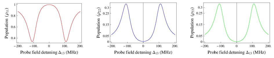
Figure 7: The population curves for the lower (Red), middle (Blue) and upper (Green) levels of the vee system are plotted as the function of probe field detuning frequency Δ13\Delta_{13} from Eq.(19a). We note that in contrast to lambda and cascade systems, at resonance both the middle and the upper levels (ρ33≠0,ρ22≠0\rho_{33}\neq 0,\rho_{22}\neq 0) are well populated while the lower level is almost empty (ρ11≈0\rho_{11}\approx 0)

Here we note that, contrast to other two configurations, a fundamental difference appears in the population dynamics of the vee system. Fig.6 shows that when EIT occurs at probe field resonance, the atomic population is being trapped in the upper and middle levels leaving the population of the lower level almost vanishing. The reason for such unusual behaviour contrary to other two systems can be understood by comparing the dark states of three systems.

The generic dark state of the three-level systems, each of which is indeed the destructive superposition of its two mutually uncoupled bare states, are given by [10],

|a0Λ>\displaystyle|a_{0}^{\Lambda}> =\displaystyle= cos⁡θΛ|1>−sin⁡θΛ|2>,\displaystyle\cos{{\theta}^{\Lambda}}|1>-\sin{{\theta}^{\Lambda}}|2>, (21a)
|a0Ξ>\displaystyle|a_{0}^{\Xi}> =\displaystyle= cos⁡θΞ|1>−sin⁡θΞ|3>,\displaystyle\cos{{\theta}^{\Xi}}|1>-\sin{{\theta}^{\Xi}}|3>, (21b)
|a0V>\displaystyle|a_{0}^{V}> =\displaystyle= cos⁡θV|2>−sin⁡θV|3>,\displaystyle\cos{{\theta}^{V}}|2>-\sin{{\theta}^{V}}|3>, (21c)

for the lambda, cascade and vee systems, respectively, where θA\theta^{A} be the mixing angle of the bare states. To get an estimate of the mixing angle we analyse the population distribution in the bare states discussed above. For the lambda system, Fig.3 shows that the accumulation of the population occurs in the lowest level (i.e., level |1>|1>) and it corresponds to θΛ≃0\theta^{\Lambda}\simeq 0 in Eq.(21a). Similar situation occurs for the cascade system for which in Eq.(21b) we have θΞ≃0\theta^{\Xi}\simeq 0. On the other hand, since the population in the vee system is equally distributed in two bare states |2>|2> and |3>|3> as evident from Fig.7, the corresponding mixing angles in Eq.(21c) are given by θV≈π4\theta^{V}\approx\frac{\pi}{4}, respectively. Thus the dark states of the three systems in Eq.(23) are given by,

|a0Λ>\displaystyle|a_{0}^{\Lambda}> ≃\displaystyle\simeq |1>,\displaystyle|1>, (22a)
|a0Ξ>\displaystyle|a_{0}^{\Xi}> ≃\displaystyle\simeq |1>,\displaystyle|1>, (22b)
|a0V>\displaystyle|a_{0}^{V}> ≃\displaystyle\simeq 12|2>−12|3>,\displaystyle\frac{1}{\sqrt{2}}|2>-\frac{1}{\sqrt{2}}|3>, (22c)

respectively, where the maximal superposition of the bare states in the vee system is clearly evident.

5 Conclusions

This paper reports a systematic study of the EIT exhibited by the lambda, cascade and vee configurations which per se are different from one another  [21]. The Optical Bloch Equation (OBE) for each system is solved to find the steady state density matrix of the desired system which eventually gives the dispersion profile, absorption coefficient and the group velocity of resonant probe field. Although all three configurations exhibit the EIT effect, but the analysis of the population curves of each system shows that the vee system is remarkably distinct from that of the lambda and cascade systems. At resonance, whole population of the lambda and cascade systems are found to be trapped in the lowermost bare state, which is indeed effectively be the dressed dark state of these systems. On the other hand, for the vee system, the dressed dark state retains its superposed character where population is equally distributed in the middle and upper states. The estimate of the mixing angle θA​(gi​j,Γi​j)\theta^{A}(g_{ij},\Gamma_{ij}) presented here is based on the numerical values of the Rabi frequencies and the decay constants when the EIT is observed at zero probe detuning. Finding the analytical expression of the angle, which determines the exact contribution of two bare states in the dark state, is possibly an open issue.

Finally a few comments about the choice of the numerical values used in this paper. Since our model is generic in nature, therefore, it is easy to validate it for other values of the numerical parameters too. In particular, we have made a numerical check of our models with the parameters used in a EIT based model of micro-switching where the controlling of the windows of the Autler-Townes doublet plays key role [27, 28]. The EIT has wide prospect of application in fabricating future quantum control devices which are capable of micro-switching, storing and processing the optical information in a micron-size cavity [29, 30, 31]. We expect that, the maximally superposed charcater of dark state of the vee system reported here may be useful to design some advanced optically controlled switching system.

Acknowledgement

SS is thankful to Department of Science and Technology, New Delhi for partial support. SS and TKD also thank S N Bose National Centre for Basic Sciences, Kolkata, for supporting their visit.

References

  • [1] Alzetta, G.; Gozzini, A.; Moi, L.; Oriols, G. Nuovo Cimento 1976, B36, 5–20.
  • [2] Arimondo, E.; Orriols, G. Nuovo Cimento Letters 1976, 17, 333–338.
  • [3] Harris, S.E. Phys. Rev. Lett. 1989, 62, 1033–1036.
  • [4] Scully, M.O.; Zhu, S.Y.; Gravrielides, A. Phys. Rev. Lett. 1989, 62, 2813–2816.
  • [5] Boller, K.; Imamoglu, A.; Harris, S. Phys. Rev. Lett. 1991, 66, 2593.
  • [6] Harris, S.E. Physics Today 1997, 50, 36–42.
  • [7] Harris, S.E.; Field, J.E.; Imamoglu, A. Phys. Rev. Lett. 1992, 64, 1107–1110.
  • [8] Harris, S.E.; Field, J.E.; Kasapi, A. Phys. Rev. A 1992, 46, R29–R32.
  • [9] Marangos, J.P. J. Modern Opt. 1998, 45, 471 – 503.
  • [10] Fleischhauer, M.; Imamoglu, A.; Marangos, J.P. Rev Mod Phys 2005, 77, 633 – 673.
  • [11] Scully, M.O. Phys. Rev. Lett. 1991, 67, 1855–1858.
  • [12] Scully, M.O.; Zhu, S.Y. Opt Commun 1992, 87, 134 – 138.
  • [13] Schmidt, H.; Imamoglu, A. Opt. Lett. 1996, 21, 1936–1938.
  • [14] See for example, M. S. Zubairy and M. O. Scully, Quantum Optics, Cambridge University Press, New York, 1994, pp.225; .
  • [15] Imamoglu, A.; Harris., S.E. Opt. Lett. 1989, 14, 1344–1346.
  • [16] Hau, L.V.; Harris, S.E.; Dutton, Z.; Behroozi, C.H. Nature 1999, 397, 594–598.
  • [17] Dutton, Z.; Slowe, N.G.C.; Hau, L.V. Europhysics News 2004, 35, 33–39.
  • [18] Kash, M.M.; Sautenkov, V.A.; Zibrov, A.S.; Hollberg, L.; Welch, G.R.; Lukin, M.D.; Rostovtsev, Y.; Fry, E.S.; Scully, M.O. Phys. Rev. Lett. 1999, 82 (Jun), 5229–5232.
  • [19] Kasapi, M.; Jain, M.; Yin, G.; Harris, S.E. Phys. Rev. Lett. 1995, 74, 2447–2450.
  • [20] Grey, H.R.; Whitley, R.M.; Jr, C.R.S. Opt. Lett. 1978, 3, 218–220.
  • [21] Sen, S.; Nath, M.R.; Dey, T.K.; Gangopadhyay, G. Ann. of Phys. 2012, 12, 224–252.
  • [22] Welch, G.R.; Padmabandu, G.G.; Fry, E.S.; Lukin, M.D.; Nikonov, D.E.; Sander, F.; Scully, M.O.; Weis, A.; Tittel, F.K. Found. Phys. 1998, 28, 621–638.
  • [23] Gea-Banacloche, J.; Li, Y.q.; Jin, S.z.; Xiao, M. Phys. Rev. A 1995, 51 (Jan), 576–584.
  • [24] Lazoudis, A.; Kirova, T.; Ahmed, E.H.; Qi, P.; Huennekens, J.; Lyyra, A.M. Phys. Rev. A 2011, 83 (Jun), 063419.
  • [25] See for example, Greiner W. and Muller B., Quantum Mechanics: Symmetries, Springer, New York, 1994, pp.217; .
  • [26] Li, Y.q.; Xiao, M. Phys. Rev. A 1995, 51 (Apr), R2703–R2706.
  • [27] Li, J.; Paraoanu, G.S.; Cicak, K.; Altomare, F.; Park, J.I.; Simmonds, R.W.; Sillanpää, M.A.; Hakonen, P.J. Phys. Rev. B 2011, 84 (Sep), 104527.
  • [28] Li, J.; Paraoanu, G.S.; Cicak, K.; Altomare, F.; Park, J.I.; Simmonds, R.W.; Sillanpää, M.A.; Hakonen, P.J. Scientific Reports 2012, 2:645 (August), 1–7.
  • [29] Turukhin, A.V.; Sudarshanam, V.S.; Shahriar, M.S.; Musser, J.A.; Ham, B.S.; Hemmer, P. Phys. Rev. Lett. 2002, 88, 023602.
  • [30] Phillips, D.F.; Fleischhaueer, A.; Mair, A.; Walsworth, R.L. Phys. Rev. Lett. 2001, 86, 783–786.
  • [31] Liu, C.; Dutton, Z.; Behroozi, C.H.; Hau, L.V. Nature 2001, 409, 490–493.
\appendices

6

For completeness, in this Appendix we shall give the elements of the steady state density matrix of three configurations obtained by solving Optical Bloch Equation. It is worth mentioning that although the OBE can be solved without taking the control field detuning to be zero, but for mathematical convenience we work with its vanishing value for all three-level systems. (We drop the symbols Λ,Ξ\Lambda,\Xi and VV appearing in the superscript of Γi​j\Gamma_{ij} and Δi​j\Delta_{ij} for the notational brevity.)

a) Lambda system:

The denominator of Eqs.(13) for the lambda configuration is given by

DΛ\displaystyle\text{D}^{\Lambda} =\displaystyle= Γ32​g136+g232​(Γ31+2​Γ32)​g134+((2​Γ31+Γ32)​g234+(Γ31+Γ32)​(2​g232+Γ32​(Γ31+Γ32))​Δ132)​g132\displaystyle\Gamma_{32}g_{13}^{6}+g_{23}^{2}\left(\Gamma_{31}+2\Gamma_{32}\right)g_{13}^{4}+\left(\left(2\Gamma_{31}+\Gamma_{32}\right)g_{23}^{4}+\left(\Gamma_{31}+\Gamma_{32}\right)\left(2g_{23}^{2}+\Gamma_{32}\left(\Gamma_{31}+\Gamma_{32}\right)\right)\Delta_{13}^{2}\right)g_{13}^{2} (23)
+g232​Γ31​(g234−2​Δ132​g232+Δ134+(Γ31+Γ32)​Δ2132)\displaystyle+g_{23}^{2}\Gamma_{31}\left(g_{23}^{4}-2\Delta_{13}^{2}g_{23}^{2}+\Delta_{13}^{4}+\left(\Gamma_{31}+\Gamma_{32}\right){}^{2}\Delta_{13}^{2}\right)

while the numerators appearing in the density matrix are,

ρN​11Λ\displaystyle\rho_{\text{N}11}^{\Lambda} =\displaystyle= g232(Γ31Δ134+Γ31(g132−2g232+(Γ31+Γ32))2Δ132+(g132+g232)(Γ32g132+g232Γ31)),\displaystyle g_{23}^{2}\left(\Gamma_{31}\Delta_{13}^{4}+\Gamma_{31}\left(g_{13}^{2}-2g_{23}^{2}+\left(\Gamma_{31}+\Gamma_{32}\right){}^{2}\right)\Delta_{13}^{2}+\left(g_{13}^{2}+g_{23}^{2}\right)\left(\Gamma_{32}g_{13}^{2}+g_{23}^{2}\Gamma_{31}\right)\right),
ρN​22Λ\displaystyle\rho_{\text{N}22}^{\Lambda} =\displaystyle= g132​(Γ32​g134+g232​(Γ31+Γ32)​g132+Γ32​(Γ31+Γ32)​Δ2132+g232​Γ32​Δ132+g234​Γ31),\displaystyle g_{13}^{2}\left(\Gamma_{32}g_{13}^{4}+g_{23}^{2}\left(\Gamma_{31}+\Gamma_{32}\right)g_{13}^{2}+\Gamma_{32}\left(\Gamma_{31}+\Gamma_{32}\right){}^{2}\Delta_{13}^{2}+g_{23}^{2}\Gamma_{32}\Delta_{13}^{2}+g_{23}^{4}\Gamma_{31}\right), (24b)
ρN​33Λ\displaystyle\rho_{\text{N}33}^{\Lambda} =\displaystyle= g132​g232​(Γ31+Γ32)​Δ132,\displaystyle g_{13}^{2}g_{23}^{2}\left(\Gamma_{31}+\Gamma_{32}\right)\Delta_{13}^{2}, (24c)
ρN​12Λ\displaystyle\rho_{\text{N}12}^{\Lambda} =\displaystyle= −g13​g23​(Γ32​g134+(Γ31+Γ32)​(g232+i​Γ32​Δ13)​g132+g232​Γ31​(g232+i⁡(Γ31+Γ32+i​Δ13)​Δ13)),\displaystyle-g_{13}g_{23}\left(\Gamma_{32}g_{13}^{4}+\left(\Gamma_{31}+\Gamma_{32}\right)\left(g_{23}^{2}+i\Gamma_{32}\Delta_{13}\right)g_{13}^{2}+g_{23}^{2}\Gamma_{31}\left(g_{23}^{2}+i\left(\Gamma_{31}+\Gamma_{32}+i\Delta_{13}\right)\Delta_{13}\right)\right),
ρN​13Λ\displaystyle\rho_{\text{N}13}^{\Lambda} =\displaystyle= g13​g232​Δ13​(Γ32​g132+g232​Γ31+i​Γ31​(Γ31+Γ32+i​Δ13)​Δ13),\displaystyle g_{13}g_{23}^{2}\Delta_{13}\left(\Gamma_{32}g_{13}^{2}+g_{23}^{2}\Gamma_{31}+i\Gamma_{31}\left(\Gamma_{31}+\Gamma_{32}+i\Delta_{13}\right)\Delta_{13}\right), (24e)
ρN​23Λ\displaystyle\rho_{\text{N}23}^{\Lambda} =\displaystyle= −g132​g23​Δ13​(Γ31​g232+Γ32​(g132−i⁡(Γ31+Γ32)​Δ13)).\displaystyle-g_{13}^{2}g_{23}\Delta_{13}\left(\Gamma_{31}g_{23}^{2}+\Gamma_{32}\left(g_{13}^{2}-i\left(\Gamma_{31}+\Gamma_{32}\right)\Delta_{13}\right)\right). (24f)

b) Cascade system:

For the Cascade system, the denominator appearing in Eq.(17) is given by

DΞ\displaystyle\text{D}^{\Xi} =\displaystyle= 2Γ21Γ32g126+{(Γ212+4Γ32Γ21+2Γ322)g232+Γ21Γ32[(Γ21+2Γ32)+2Δ122]}g124\displaystyle 2\Gamma_{21}\Gamma_{32}g_{12}^{6}+\left\{\left(\Gamma_{21}^{2}+4\Gamma_{32}\Gamma_{21}+2\Gamma_{32}^{2}\right)g_{23}^{2}+\Gamma_{21}\Gamma_{32}\left[\left(\Gamma_{21}+2\Gamma_{32}\right){}^{2}+\Delta_{12}^{2}\right]\right\}g_{12}^{4} (25)
+[(2Γ212+3Γ32Γ21+2Γ322)g234+{(2Γ212+4Γ32Γ21+Γ322)Δ122\displaystyle+\left[\left(2\Gamma_{21}^{2}+3\Gamma_{32}\Gamma_{21}+2\Gamma_{32}^{2}\right)g_{23}^{4}+\left\{\left(2\Gamma_{21}^{2}+4\Gamma_{32}\Gamma_{21}+\Gamma_{32}^{2}\right)\Delta_{12}^{2}\right.\right.
+Γ32(4Γ213+7Γ32Γ212+6Γ322Γ21+2Γ323)}g232+2Γ21Γ32(Γ21+Γ32){(Γ21+2Γ32)Δ122\displaystyle\left.\left.+\Gamma_{32}\left(4\Gamma_{21}^{3}+7\Gamma_{32}\Gamma_{21}^{2}+6\Gamma_{32}^{2}\Gamma_{21}+2\Gamma_{32}^{3}\right)\right\}g_{23}^{2}+2\Gamma_{21}\Gamma_{32}\left(\Gamma_{21}+\Gamma_{32}\right)\left\{\left(\Gamma_{21}+2\Gamma_{32}\right)\Delta_{12}^{2}\right.\right.
+Γ32(Γ212+Γ32Γ21+Γ322)}]g122+Γ21(Γ21+Γ32){g232+Γ32(Γ21+Γ32)}\displaystyle\left.\left.+\Gamma_{32}\left(\Gamma_{21}^{2}+\Gamma_{32}\Gamma_{21}+\Gamma_{32}^{2}\right)\right\}\right]g_{12}^{2}+\Gamma_{21}\left(\Gamma_{21}+\Gamma_{32}\right)\left\{g_{23}^{2}+\Gamma_{32}\left(\Gamma_{21}+\Gamma_{32}\right)\right\}
{g234+2​(Γ21​Γ32−Δ122)​g232+(Γ212+Δ122)​(Γ322+Δ122)},\displaystyle\left\{g_{23}^{4}+2\left(\Gamma_{21}\Gamma_{32}-\Delta_{12}^{2}\right)g_{23}^{2}+\left(\Gamma_{21}^{2}+\Delta_{12}^{2}\right)\left(\Gamma_{32}^{2}+\Delta_{12}^{2}\right)\right\},

and the terms in the numerator are given by,

ρN​11Ξ\displaystyle\rho_{\text{N}11}^{\Xi} =\displaystyle= Γ21​Γ32​g126+Γ32​{(Γ21+Γ32)​g232+Γ21​(Γ212+2​Γ32​Γ21+2​Γ322+Δ122)}​g124\displaystyle\Gamma_{21}\Gamma_{32}g_{12}^{6}+\Gamma_{32}\left\{\left(\Gamma_{21}+\Gamma_{32}\right)g_{23}^{2}+\Gamma_{21}\left(\Gamma_{21}^{2}+2\Gamma_{32}\Gamma_{21}+2\Gamma_{32}^{2}+\Delta_{12}^{2}\right)\right\}g_{12}^{4} (26a)
+[Γ212g234+{(Γ212+3Γ32Γ21+Γ322)Δ122+Γ32(3Γ213+3Γ32Γ212+2Γ322Γ21+Γ323)}g232\displaystyle+\left[\Gamma_{21}^{2}g_{23}^{4}+\left\{\left(\Gamma_{21}^{2}+3\Gamma_{32}\Gamma_{21}+\Gamma_{32}^{2}\right)\Delta_{12}^{2}+\Gamma_{32}\left(3\Gamma_{21}^{3}+3\Gamma_{32}\Gamma_{21}^{2}+2\Gamma_{32}^{2}\Gamma_{21}+\Gamma_{32}^{3}\right)\right\}g_{23}^{2}\right.
+Γ21Γ32(Γ21+Γ32){(Γ21+3Γ32)Δ122+Γ32(2Γ212+Γ32Γ21+Γ322)}]g122+Γ21(Γ21+Γ32)\displaystyle\left.+\Gamma_{21}\Gamma_{32}\left(\Gamma_{21}+\Gamma_{32}\right)\left\{\left(\Gamma_{21}+3\Gamma_{32}\right)\Delta_{12}^{2}+\Gamma_{32}\left(2\Gamma_{21}^{2}+\Gamma_{32}\Gamma_{21}+\Gamma_{32}^{2}\right)\right\}\right]g_{12}^{2}+\Gamma_{21}\left(\Gamma_{21}+\Gamma_{32}\right)
{g232+Γ32​(Γ21+Γ32)}​{g234+2​(Γ21​Γ32−Δ122)​g232+(Γ212+Δ122)​(Γ322+Δ122)},\displaystyle\left\{g_{23}^{2}+\Gamma_{32}\left(\Gamma_{21}+\Gamma_{32}\right)\right\}\left\{g_{23}^{4}+2\left(\Gamma_{21}\Gamma_{32}-\Delta_{12}^{2}\right)g_{23}^{2}+\left(\Gamma_{21}^{2}+\Delta_{12}^{2}\right)\left(\Gamma_{32}^{2}+\Delta_{12}^{2}\right)\right\},
ρN​22Ξ\displaystyle\rho_{\text{N}22}^{\Xi} =\displaystyle= g122[Γ21Γ32g124+Γ32{(2Γ21+Γ32)g232+2Γ21Γ32(Γ21+Γ32)}g122\displaystyle g_{12}^{2}\left[\Gamma_{21}\Gamma_{32}g_{12}^{4}+\Gamma_{32}\left\{\left(2\Gamma_{21}+\Gamma_{32}\right)g_{23}^{2}+2\Gamma_{21}\Gamma_{32}\left(\Gamma_{21}+\Gamma_{32}\right)\right\}g_{12}^{2}\right. (26b)
+(Γ21+Γ32){g232+Γ32(Γ21+Γ32)}{Γ32g232+Γ21(Γ322+Δ122)}],\displaystyle\left.+\left(\Gamma_{21}+\Gamma_{32}\right)\left\{g_{23}^{2}+\Gamma_{32}\left(\Gamma_{21}+\Gamma_{32}\right)\right\}\left\{\Gamma_{32}g_{23}^{2}+\Gamma_{21}\left(\Gamma_{32}^{2}+\Delta_{12}^{2}\right)\right\}\right],
ρN​33Ξ\displaystyle\rho_{\text{N}33}^{\Xi} =\displaystyle= g122​g232​(Γ21+Γ32)​{Γ21​g122+(Γ21+Γ32)​(g232+Γ21​Γ32)},\displaystyle g_{12}^{2}g_{23}^{2}\left(\Gamma_{21}+\Gamma_{32}\right)\left\{\Gamma_{21}g_{12}^{2}+\left(\Gamma_{21}+\Gamma_{32}\right)\left(g_{23}^{2}+\Gamma_{21}\Gamma_{32}\right)\right\}, (26c)
ρN​12Ξ\displaystyle\rho_{\text{N}12}^{\Xi} =\displaystyle= ig12[Γ21Γ32(Γ21+iΔ12)g124+Γ32{(2Γ21+Γ32)g232+2Γ21Γ32(Γ21+Γ32)}\displaystyle ig_{12}\left[\Gamma_{21}\Gamma_{32}\left(\Gamma_{21}+i\Delta_{12}\right)g_{12}^{4}+\Gamma_{32}\left\{\left(2\Gamma_{21}+\Gamma_{32}\right)g_{23}^{2}+2\Gamma_{21}\Gamma_{32}\left(\Gamma_{21}+\Gamma_{32}\right)\right\}\right. (26d)
(Γ21+i​Δ12)​g122+Γ21​(Γ21+Γ32)​{g232+Γ32​(Γ21+Γ32)}\displaystyle\left.\left(\Gamma_{21}+i\Delta_{12}\right)g_{12}^{2}+\Gamma_{21}\left(\Gamma_{21}+\Gamma_{32}\right)\left\{g_{23}^{2}+\Gamma_{32}\left(\Gamma_{21}+\Gamma_{32}\right)\right\}\right.
{g232+(Γ21+iΔ12)(Γ32+iΔ12)}(Γ32−iΔ12)],\displaystyle\left.\left\{g_{23}^{2}+\left(\Gamma_{21}+i\Delta_{12}\right)\left(\Gamma_{32}+i\Delta_{12}\right)\right\}\left(\Gamma_{32}-i\Delta_{12}\right)\right],
ρN​13Ξ\displaystyle\rho_{\text{N}13}^{\Xi} =\displaystyle= g12g23[Γ21Γ32g124+{−Γ32Γ213+Γ323Γ21+g232(−Γ212+Γ32Γ21+Γ322)}g122\displaystyle g_{12}g_{23}\left[\Gamma_{21}\Gamma_{32}g_{12}^{4}+\left\{-\Gamma_{32}\Gamma_{21}^{3}+\Gamma_{32}^{3}\Gamma_{21}+g_{23}^{2}\left(-\Gamma_{21}^{2}+\Gamma_{32}\Gamma_{21}+\Gamma_{32}^{2}\right)\right\}g_{12}^{2}\right. (26e)
−Γ21(Γ21+Γ32){g232+Γ32(Γ21+Γ32)}{g232+(Γ21+iΔ12)(Γ32+iΔ12)}],\displaystyle\left.-\Gamma_{21}\left(\Gamma_{21}+\Gamma_{32}\right)\left\{g_{23}^{2}+\Gamma_{32}\left(\Gamma_{21}+\Gamma_{32}\right)\right\}\left\{g_{23}^{2}+\left(\Gamma_{21}+i\Delta_{12}\right)\left(\Gamma_{32}+i\Delta_{12}\right)\right\}\right],
ρN​23Ξ\displaystyle\rho_{\text{N}23}^{\Xi} =\displaystyle= ig122g23(Γ21+Γ32)[Γ21Γ32g122+Γ32(Γ21+Γ32)(g232+Γ21Γ32)\displaystyle ig_{12}^{2}g_{23}\left(\Gamma_{21}+\Gamma_{32}\right)\left[\Gamma_{21}\Gamma_{32}g_{12}^{2}+\Gamma_{32}\left(\Gamma_{21}+\Gamma_{32}\right)\left(g_{23}^{2}+\Gamma_{21}\Gamma_{32}\right)\right. (26f)
+iΓ21{g232+Γ32(Γ21+Γ32)}Δ12].\displaystyle\left.+i\Gamma_{21}\left\{g_{23}^{2}+\Gamma_{32}\left(\Gamma_{21}+\Gamma_{32}\right)\right\}\Delta_{12}\right].

c) Vee system:

The denominator appearing in Eq.(21) is given by

DV\displaystyle\text{D}^{\text{V}} =\displaystyle= 2Γ21Γ31g126+[2(Γ212+Γ31Γ21+Γ312)g132+Γ21Γ31{(Γ21+2Γ31)−24Δ132}]g124\displaystyle 2\Gamma_{21}\Gamma_{31}g_{12}^{6}+\left[2\left(\Gamma_{21}^{2}+\Gamma_{31}\Gamma_{21}+\Gamma_{31}^{2}\right)g_{13}^{2}+\Gamma_{21}\Gamma_{31}\left\{\left(\Gamma_{21}+2\Gamma_{31}\right){}^{2}-4\Delta_{13}^{2}\right\}\right]g_{12}^{4} (27)
+[2Γ21Γ31Δ134+{(Γ212+6Γ31Γ21+2Γ312)g132+4Γ21Γ312(Γ21+Γ31)}Δ132\displaystyle+\left[2\Gamma_{21}\Gamma_{31}\Delta_{13}^{4}+\left\{\left(\Gamma_{21}^{2}+6\Gamma_{31}\Gamma_{21}+2\Gamma_{31}^{2}\right)g_{13}^{2}+4\Gamma_{21}\Gamma_{31}^{2}\left(\Gamma_{21}+\Gamma_{31}\right)\right\}\Delta_{13}^{2}\right.
+2(g132+Γ312)(Γ212+Γ31Γ21+Γ312){g132+Γ21(Γ21+Γ31)}]g122\displaystyle\left.+2\left(g_{13}^{2}+\Gamma_{31}^{2}\right)\left(\Gamma_{21}^{2}+\Gamma_{31}\Gamma_{21}+\Gamma_{31}^{2}\right)\left\{g_{13}^{2}+\Gamma_{21}\left(\Gamma_{21}+\Gamma_{31}\right)\right\}\right]g_{12}^{2}
+Γ21Γ31(2g132+Γ312+Δ132){(g132+Γ21(Γ21+Γ31))+2Γ212Δ132},\displaystyle+\Gamma_{21}\Gamma_{31}\left(2g_{13}^{2}+\Gamma_{31}^{2}+\Delta_{13}^{2}\right)\left\{\left(g_{13}^{2}+\Gamma_{21}\left(\Gamma_{21}+\Gamma_{31}\right)\right){}^{2}+\Gamma_{21}^{2}\Delta_{13}^{2}\right\},

and other terms in the numerator of the density matrix are,

ρN​11V\displaystyle\rho_{\text{N}11}^{\text{V}} =\displaystyle= Γ21​Γ31​g126+{(Γ212+Γ31​Γ21+Γ312)​g132+Γ21​Γ31​(Γ212+2​Γ31​Γ21+2​Γ312−2​Δ132)}​g124\displaystyle\Gamma_{21}\Gamma_{31}g_{12}^{6}+\left\{\left(\Gamma_{21}^{2}+\Gamma_{31}\Gamma_{21}+\Gamma_{31}^{2}\right)g_{13}^{2}+\Gamma_{21}\Gamma_{31}\left(\Gamma_{21}^{2}+2\Gamma_{31}\Gamma_{21}+2\Gamma_{31}^{2}-2\Delta_{13}^{2}\right)\right\}g_{12}^{4} (28a)
+[(Γ212+Γ31Γ21+Γ312)g134+{Γ214+2Γ31Γ213+4Γ312Γ212+2Γ313Γ21+Γ314\displaystyle+\left[\left(\Gamma_{21}^{2}+\Gamma_{31}\Gamma_{21}+\Gamma_{31}^{2}\right)g_{13}^{4}+\left\{\Gamma_{21}^{4}+2\Gamma_{31}\Gamma_{21}^{3}+4\Gamma_{31}^{2}\Gamma_{21}^{2}+2\Gamma_{31}^{3}\Gamma_{21}+\Gamma_{31}^{4}\right.\right.
+Γ31(2Γ21+Γ31)Δ132}g132+Γ21Γ31{2Γ31Γ213+(3Γ312−Δ132)Γ212\displaystyle\left.\left.+\Gamma_{31}\left(2\Gamma_{21}+\Gamma_{31}\right)\Delta_{13}^{2}\right\}g_{13}^{2}+\Gamma_{21}\Gamma_{31}\left\{2\Gamma_{31}\Gamma_{21}^{3}+\left(3\Gamma_{31}^{2}-\Delta_{13}^{2}\right)\Gamma_{21}^{2}\right.\right.
+2Γ31(Γ312+Δ132)Γ21+(Γ312+Δ132)}2]g122+Γ21Γ31(g132+Γ312+Δ132)\displaystyle\left.\left.+2\Gamma_{31}\left(\Gamma_{31}^{2}+\Delta_{13}^{2}\right)\Gamma_{21}+\left(\Gamma_{31}^{2}+\Delta_{13}^{2}\right){}^{2}\right\}\right]g_{12}^{2}+\Gamma_{21}\Gamma_{31}\left(g_{13}^{2}+\Gamma_{31}^{2}+\Delta_{13}^{2}\right)
{(g132+Γ21(Γ21+Γ31))+2Γ212Δ132},\displaystyle\left\{\left(g_{13}^{2}+\Gamma_{21}\left(\Gamma_{21}+\Gamma_{31}\right)\right){}^{2}+\Gamma_{21}^{2}\Delta_{13}^{2}\right\},
ρN​22V\displaystyle\rho_{\text{N}22}^{\text{V}} =\displaystyle= g122[Γ21Γ31g124+{(Γ212+Γ312)g132+2Γ21Γ31(Γ31(Γ21+Γ31)−Δ132)}g122\displaystyle g_{12}^{2}\left[\Gamma_{21}\Gamma_{31}g_{12}^{4}+\left\{\left(\Gamma_{21}^{2}+\Gamma_{31}^{2}\right)g_{13}^{2}+2\Gamma_{21}\Gamma_{31}\left(\Gamma_{31}\left(\Gamma_{21}+\Gamma_{31}\right)-\Delta_{13}^{2}\right)\right\}g_{12}^{2}\right. (28b)
+Γ31{Γ21g134+[Γ213+Γ31Γ212+Γ312Γ21+Γ313+(3Γ21+Γ31)Δ132]g132\displaystyle\left.+\Gamma_{31}\left\{\Gamma_{21}g_{13}^{4}+\left[\Gamma_{21}^{3}+\Gamma_{31}\Gamma_{21}^{2}+\Gamma_{31}^{2}\Gamma_{21}+\Gamma_{31}^{3}+\left(3\Gamma_{21}+\Gamma_{31}\right)\Delta_{13}^{2}\right]g_{13}^{2}\right.\right.
+Γ21(Γ312+Δ132)[(Γ21+Γ31)+2Δ132]}],\displaystyle\left.\left.+\Gamma_{21}\left(\Gamma_{31}^{2}+\Delta_{13}^{2}\right)\left[\left(\Gamma_{21}+\Gamma_{31}\right){}^{2}+\Delta_{13}^{2}\right]\right\}\right],
ρN​33V\displaystyle\rho_{\text{N}33}^{\text{V}} =\displaystyle= g132[Γ21Γ31g124+{(Γ212+Γ312)g132+Γ21(Γ21+Γ31)(Γ212+Γ312+Δ132)}g122\displaystyle g_{13}^{2}\left[\Gamma_{21}\Gamma_{31}g_{12}^{4}+\left\{\left(\Gamma_{21}^{2}+\Gamma_{31}^{2}\right)g_{13}^{2}+\Gamma_{21}\left(\Gamma_{21}+\Gamma_{31}\right)\left(\Gamma_{21}^{2}+\Gamma_{31}^{2}+\Delta_{13}^{2}\right)\right\}g_{12}^{2}\right. (28c)
+Γ21Γ31{(g132+Γ21(Γ21+Γ31))+2Γ212Δ132}],\displaystyle\left.+\Gamma_{21}\Gamma_{31}\left\{\left(g_{13}^{2}+\Gamma_{21}\left(\Gamma_{21}+\Gamma_{31}\right)\right){}^{2}+\Gamma_{21}^{2}\Delta_{13}^{2}\right\}\right],
ρN​12V\displaystyle\rho_{\text{N}12}^{\text{V}} =\displaystyle= ig12[Γ212Γ31g124+{(Γ213+Γ312Γ21+2iΓ312Δ13)g132+2Γ212Γ31[Γ31(Γ21+Γ31)\displaystyle ig_{12}\left[\Gamma_{21}^{2}\Gamma_{31}g_{12}^{4}+\left\{\left(\Gamma_{21}^{3}+\Gamma_{31}^{2}\Gamma_{21}+2i\Gamma_{31}^{2}\Delta_{13}\right)g_{13}^{2}+2\Gamma_{21}^{2}\Gamma_{31}\left[\Gamma_{31}\left(\Gamma_{21}+\Gamma_{31}\right)\right.\right.\right. (28d)
−Δ132]}g122+Γ21Γ31{g132+Γ21(Γ21+Γ31−iΔ13)}{(Γ21+2iΔ13)g132\displaystyle\left.\left.\left.-\Delta_{13}^{2}\right]\right\}g_{12}^{2}+\Gamma_{21}\Gamma_{31}\left\{g_{13}^{2}+\Gamma_{21}\left(\Gamma_{21}+\Gamma_{31}-i\Delta_{13}\right)\right\}\left\{\left(\Gamma_{21}+2i\Delta_{13}\right)g_{13}^{2}\right.\right.
+(Γ21+Γ31+iΔ13)(Γ312+Δ132)}],\displaystyle\left.\left.+\left(\Gamma_{21}+\Gamma_{31}+i\Delta_{13}\right)\left(\Gamma_{31}^{2}+\Delta_{13}^{2}\right)\right\}\right],
ρN​13V\displaystyle\rho_{\text{N}13}^{\text{V}} =\displaystyle= ig13[Γ21Γ31(Γ31−iΔ13)g124+{iΓ21Γ31Δ133+Γ21Γ31(Γ21+Γ31)Δ132\displaystyle ig_{13}\left[\Gamma_{21}\Gamma_{31}\left(\Gamma_{31}-i\Delta_{13}\right)g_{12}^{4}+\left\{i\Gamma_{21}\Gamma_{31}\Delta_{13}^{3}+\Gamma_{21}\Gamma_{31}\left(\Gamma_{21}+\Gamma_{31}\right)\Delta_{13}^{2}\right.\right. (28e)
+i(g132+Γ21Γ31)(Γ312−Γ212)Δ13+Γ31(Γ212+Γ312)[g132+Γ21(Γ21+Γ31)]}g122\displaystyle\left.\left.+i\left(g_{13}^{2}+\Gamma_{21}\Gamma_{31}\right)\left(\Gamma_{31}^{2}-\Gamma_{21}^{2}\right)\Delta_{13}+\Gamma_{31}\left(\Gamma_{21}^{2}+\Gamma_{31}^{2}\right)\left[g_{13}^{2}+\Gamma_{21}\left(\Gamma_{21}+\Gamma_{31}\right)\right]\right\}g_{12}^{2}\right.
+Γ21Γ31(Γ31+iΔ13){[g132+Γ21(Γ21+Γ31)]+2Γ212Δ132}],\displaystyle\left.+\Gamma_{21}\Gamma_{31}\left(\Gamma_{31}+i\Delta_{13}\right)\left\{\left[g_{13}^{2}+\Gamma_{21}\left(\Gamma_{21}+\Gamma_{31}\right)\right]{}^{2}+\Gamma_{21}^{2}\Delta_{13}^{2}\right\}\right],
ρN​23V\displaystyle\rho_{\text{N}23}^{\text{V}} =\displaystyle= g12g13[Γ21Γ31g124+{(Γ212+Γ312)g132+Γ21Γ31[Γ212+2Γ31Γ21+(Γ31+iΔ13)]2}g122\displaystyle g_{12}g_{13}\left[\Gamma_{21}\Gamma_{31}g_{12}^{4}+\left\{\left(\Gamma_{21}^{2}+\Gamma_{31}^{2}\right)g_{13}^{2}+\Gamma_{21}\Gamma_{31}\left[\Gamma_{21}^{2}+2\Gamma_{31}\Gamma_{21}+\left(\Gamma_{31}+i\Delta_{13}\right){}^{2}\right]\right\}g_{12}^{2}\right.
+Γ21Γ31{g132+Γ21(Γ21+Γ31+iΔ13)}{g132+Δ132+Γ31(Γ21+Γ31)+iΓ21Δ13}].\displaystyle\left.+\Gamma_{21}\Gamma_{31}\left\{g_{13}^{2}+\Gamma_{21}\left(\Gamma_{21}+\Gamma_{31}+i\Delta_{13}\right)\right\}\left\{g_{13}^{2}+\Delta_{13}^{2}+\Gamma_{31}\left(\Gamma_{21}+\Gamma_{31}\right)+i\Gamma_{21}\Delta_{13}\right\}\right].