跳到论文正文
W Papers独立论文阅读器 arXiv:1305.5029 论文正文 计算阅读时间 · 0%
引用这篇论文根据当前论文元数据生成,正式投稿前建议核对。


License: arXiv.org perpetual non-exclusive license
arXiv:1305.5029v2 [math.ST] 29 Apr 2014

Divide and Conquer Kernel Ridge Regression:
A Distributed Algorithm with Minimax Optimal Rates

Yuchen Zhang 1 John C. Duchi1 Martin J. Wainwright1,2
yuczhang@eecs.berkeley.edu jduchi@eecs.berkeley.edu wainwrig@stat.berkeley.edu
Department of Statistics1 Department of Electrical Engineering and Computer Science2
UC Berkeley, Berkeley, CA 94720

May 2013

Abstract

We establish optimal convergence rates for a decomposition-based scalable approach to kernel ridge regression. The method is simple to describe: it randomly partitions a dataset of size NN into mm subsets of equal size, computes an independent kernel ridge regression estimator for each subset, then averages the local solutions into a global predictor. This partitioning leads to a substantial reduction in computation time versus the standard approach of performing kernel ridge regression on all NN samples. Our two main theorems establish that despite the computational speed-up, statistical optimality is retained: as long as mm is not too large, the partition-based estimator achieves the statistical minimax rate over all estimators using the set of NN samples. As concrete examples, our theory guarantees that the number of processors mm may grow nearly linearly for finite-rank kernels and Gaussian kernels and polynomially in NN for Sobolev spaces, which in turn allows for substantial reductions in computational cost. We conclude with experiments on both simulated data and a music-prediction task that complement our theoretical results, exhibiting the computational and statistical benefits of our approach.

1 Introduction

In non-parametric regression, the statistician receives NN samples of the form {(xi,yi)}i=1N\{(x_{i},y_{i})\}_{i=1}^{N}, where each xi∈𝒳x_{i}\in\mathcal{X} is a covariate and yi∈ℝy_{i}\in\mathbb{R} is a real-valued response, and the samples are drawn i.i.d. from some unknown joint distribution ℙ\mathbb{P} over 𝒳×ℝ\mathcal{X}\times\mathbb{R}. The goal is to estimate a function f^:𝒳→ℝ\widehat{f}:\mathcal{X}\rightarrow\mathbb{R} that can be used to predict future responses based on observing only the covariates. Frequently, the quality of an estimate f^\widehat{f} is measured in terms of the mean-squared prediction error 𝔼​[(f^​(X)−Y)2]\mathbb{E}[(\widehat{f}(X)-Y)^{2}], in which case the conditional expectation f∗​(x)=𝔼⁡[Y∣X=x]f^{*}(x)=\mathbb{E}[Y\mid X=x] is optimal. The problem of non-parametric regression is a classical one, and a researchers have studied a wide range of estimators (see, e.g., the books [11, 32, 30]). One class of methods, known as regularized MM-estimators [30], are based on minimizing the combination of a data-dependent loss function with a regularization term. The focus of this paper is a popular MM-estimator that combines the least-squares loss with a squared Hilbert norm penalty for regularization. When working in a reproducing kernel Hilbert space (RKHS), the resulting method is known as kernel ridge regression, and is widely used in practice [12, 26]. Past work has established bounds on the estimation error for RKHS-based methods [16, 20, 30, 35, e.g.,], which have been refined and extended in more recent work [27, e.g.,].

Although the statistical aspects of kernel ridge regression (KRR) are well-understood, the computation of the KRR estimate can be challenging for large datasets. In a standard implementation [24], the kernel matrix must be inverted, which requires costs 𝒪⁡(N3)\mathcal{O}(N^{3}) and 𝒪⁡(N2)\mathcal{O}(N^{2}) in time and memory respectively. Such scalings are prohibitive when the sample size NN is large. As a consequence, approximations have been designed to avoid the expense of finding an exact minimizer. One family of approaches is based on low-rank approximation of the kernel matrix; examples include kernel PCA [25], the incomplete Cholesky decomposition [9], or Nyström sampling [33]. These methods reduce the time complexity to 𝒪⁡(d​N2)\mathcal{O}(dN^{2}) or 𝒪⁡(d2​N)\mathcal{O}(d^{2}N), where d≪Nd\ll N is the preserved rank. The associated prediction error has only been studied very recently. Concurrent work by Bach [1] establishes conditions on the maintained rank that still guarantee optimal convergence rates; see the discussion for more detail. A second line of research has considered early-stopping of iterative optimization algorithms for KRR, including gradient descent [34, 22] and conjugate gradient methods [6], where early-stopping provides regularization against over-fitting and improves run-time. If the algorithm stops after tt iterations, the aggregate time complexity is 𝒪⁡(t​N2)\mathcal{O}(tN^{2}).

In this work, we study a different decomposition-based approach. The algorithm is appealing in its simplicity: we partition the dataset of size NN randomly into mm equal sized subsets, and we compute the kernel ridge regression estimate f^i\widehat{f}_{i} for each of the i=1,…,mi=1,\ldots,m subsets independently, with a careful choice of the regularization parameter. The estimates are then averaged via f¯=(1/m)​∑i=1mf^i\bar{f}=(1/m)\sum_{i=1}^{m}\widehat{f}_{i}. Our main theoretical result gives conditions under which the average f¯\bar{f} achieves the minimax rate of convergence over the underlying Hilbert space. Even using naive implementations of KRR, this decomposition gives time and memory complexity scaling as 𝒪⁡(N3/m2)\mathcal{O}(N^{3}/m^{2}) and 𝒪⁡(N2/m2)\mathcal{O}(N^{2}/m^{2}), respectively. Moreover, our approach dovetails naturally with parallel and distributed computation: we are guaranteed superlinear speedup with mm parallel processors (though we must still communicate the function estimates from each processor). Divide-and-conquer approaches have been studied by several authors, including McDonald et al. [19] for perceptron-based algorithms, Kleiner et al. [15] in distributed versions of the bootstrap, and Zhang et al. [36] for parametric smooth convex optimization problems. This paper demonstrates the potential benefits of divide-and-conquer approaches for nonparametric and infinite-dimensional regression problems.

One difficulty in solving each of the sub-problems independently is how to choose the regularization parameter. Due to the infinite-dimensional nature of non-parametric problems, the choice of regularization parameter must be made with care [12, e.g.,]. An interesting consequence of our theoretical analysis is in demonstrating that, even though each partitioned sub-problem is based only on the fraction N/mN/m of samples, it is nonetheless essential to regularize the partitioned sub-problems as though they had all NN samples. Consequently, from a local point of view, each sub-problem is under-regularized. This “under-regularization” allows the bias of each local estimate to be very small, but it causes a detrimental blow-up in the variance. However, as we prove, the mm-fold averaging underlying the method reduces variance enough that the resulting estimator f¯\bar{f} still attains optimal convergence rate.

The remainder of this paper is organized as follows. We begin in Section 2 by providing background on the kernel ridge regression estimate and discussing the assumptions that underlie our analysis. In Section 3, we present our main theorems on the mean-squared error between the averaged estimate f¯\bar{f} and the optimal regression function f∗f^{*}. We provide both a result when the regression function f∗f^{*} belongs to the Hilbert space ℋ\mathcal{H} associated with the kernel, as well as a more general oracle inequality that holds for a general f∗f^{*}. We then provide several corollaries that exhibit concrete consequences of the results, including convergence rates of r/Nr/N for kernels with finite rank rr, and convergence rates of N−2ν/(2ν+1)N^{-2\nu/(2\nu+1)} for estimation of functionals in a Sobolev space with ν\nu-degrees of smoothness. As we discuss, both of these estimation rates are minimax-optimal and hence unimprovable. We devote Sections 4 and 5 to the proofs of our results, deferring more technical aspects of the analysis to appendices. Lastly, we present simulation results in Section 6.1 to further explore our theoretical results, while Section 6.2 contains experiments with a reasonably large music prediction experiment.

2 Background and problem formulation

We begin with the background and notation required for a precise statement of our problem.

2.1 Reproducing kernels

The method of kernel ridge regression is based on the idea of a reproducing kernel Hilbert space. We provide only a very brief coverage of the basics here, referring the reader to one of the many books on the topic (e.g., [31, 26, 3, 10]) for further details. Any symmetric and positive semidefinite kernel function K:𝒳×𝒳→ℝK:\mathcal{X}\times\mathcal{X}\to\mathbb{R} defines a reproducing kernel Hilbert space (RKHS for short). For a given distribution ℙ\mathbb{P} on 𝒳\mathcal{X}, the Hilbert space is strictly contained within L2​(ℙ)L^{2}(\mathbb{P}). For each x∈𝒳x\in\mathcal{X}, the function z↦K⁡(z,x)z\mapsto K(z,x) is contained with the Hilbert space ℋ\mathcal{H}; moreover, the Hilbert space is endowed with an inner product ⟨⋅,⋅⟩ℋ\left\langle\cdot,\cdot\right\rangle_{\mathcal{H}} such that K⁡(⋅,x)K(\cdot,x) acts as the representer of evaluation, meaning

⟨f,K⁡(x,⋅)⟩ℋ=f⁡(x)​for ​f∈ℋ.\left\langle f,K(x,\cdot)\right\rangle_{\mathcal{H}}=f(x)~~~\mbox{for~}f\in\mathcal{H}. (1)

We let ‖g‖ℋ:=⟨g,g⟩ℋ\left\|{g}\right\|_{\mathcal{H}}:=\sqrt{\left\langle g,g\right\rangle_{\mathcal{H}}} denote the norm in ℋ\mathcal{H}, and similarly ‖g‖2:=(∫𝒳g​(x)2​𝑑ℙ​(x))1/2\left\|{g}\right\|_{2}:=(\int_{\mathcal{X}}g(x)^{2}d\mathbb{P}(x))^{1/2} denotes the norm in L2​(ℙ){L^{2}(\mathbb{P})}. Under suitable regularity conditions, Mercer’s theorem guarantees that the kernel has an eigen-expansion of the form

K⁡(x,x′)=∑j=1∞μj​ϕj​(x)​ϕj​(x′),K(x,x^{\prime})=\sum_{j=1}^{\infty}\mu_{j}\phi_{j}(x)\phi_{j}(x^{\prime}),

where μ1≥μ2≥⋯≥0\mu_{1}\geq\mu_{2}\geq\dots\geq 0 are a non-negative sequence of eigenvalues, and {ϕj}j=1∞\{\phi_{j}\}_{j=1}^{\infty} is an orthonormal basis for L2​(ℙ){L^{2}(\mathbb{P})}.

From the reproducing relation (1), we have ⟨ϕj,ϕj⟩ℋ=1/μj\langle\phi_{j},\phi_{j}\rangle_{\mathcal{H}}=1/\mu_{j} for any jj and ⟨ϕj,ϕj′⟩ℋ=0\langle\phi_{j},\phi_{j^{\prime}}\rangle_{\mathcal{H}}=0 for any j≠j′j\neq j^{\prime}. For any f∈ℋf\in\mathcal{H}, by defining the basis coefficients θj=⟨f,ϕj⟩L2​(ℙ)\theta_{j}=\left\langle{f},{\phi_{j}}\right\rangle_{L^{2}(\mathbb{P})} for j=1,2,…j=1,2,\ldots, we can expand the function in terms of these coefficients as f=∑j=1∞θj​ϕjf=\sum_{j=1}^{\infty}\theta_{j}\phi_{j}, and simple calculations show that

‖f‖22=∫𝒳f2​(x)​𝑑ℙ​(x)=∑j=1∞θj2,and​‖f‖ℋ2=⟨f,f⟩=∑j=1∞θj2μj.\left\|{f}\right\|_{2}^{2}=\int_{\mathcal{X}}f^{2}(x)d\mathbb{P}(x)=\sum_{j=1}^{\infty}\theta_{j}^{2},~~~\mbox{and}~~~\left\|{f}\right\|_{\mathcal{H}}^{2}=\left\langle f,f\right\rangle=\sum_{j=1}^{\infty}\frac{\theta_{j}^{2}}{\mu_{j}}.

Consequently, we see that the RKHS can be viewed as an elliptical subset of the sequence space ℓ2​(ℕ)\ell^{2}(\mathbb{N}) as defined by the non-negative eigenvalues {μj}j=1∞\{\mu_{j}\}_{j=1}^{\infty}.

2.2 Kernel ridge regression

Suppose that we are given a data set {(xi,yi)}i=1N\{(x_{i},y_{i})\}_{i=1}^{N} consisting of NN i.i.d. samples drawn from an unknown distribution ℙ\mathbb{P} over 𝒳×ℝ\mathcal{X}\times\mathbb{R}, and our goal is to estimate the function that minimizes the mean-squared error 𝔼⁡[(f⁡(X)−Y)2]\mathbb{E}[(f(X)-Y)^{2}], where the expectation is taken jointly over (X,Y)(X,Y) pairs. It is well-known that the optimal function is the conditional mean f∗​(x):=𝔼⁡[Y∣X=x]f^{*}(x):\,=\mathbb{E}[Y\mid X=x]. In order to estimate the unknown function f∗f^{*}, we consider an MM-estimator that is based on minimizing a combination of the least-squares loss defined over the dataset with a weighted penalty based on the squared Hilbert norm,

f^\displaystyle\widehat{f} :=argminf∈ℋ{1N​∑i=1N(f⁡(xi)−yi)2+λ​‖f‖ℋ2},\displaystyle:=\mathop{\rm argmin}_{f\in\mathcal{H}}\bigg\{\frac{1}{N}\sum_{i=1}^{N}\left(f(x_{i})-y_{i}\right)^{2}+\lambda\left\|{f}\right\|_{\mathcal{H}}^{2}\bigg\}, (2)

where λ>0\lambda>0 is a regularization parameter. When ℋ\mathcal{H} is a reproducing kernel Hilbert space, then the estimator (2) is known as the kernel ridge regression estimate, or KRR for short. It is a natural generalization of the ordinary ridge regression estimate [13] to the non-parametric setting.

By the representer theorem for reproducing kernel Hilbert spaces [31], any solution to the KRR program (2) must belong to the linear span of the kernel functions {K⁡(⋅,xi),i=1,…,N}\{K(\cdot,x_{i}),\,i=1,\ldots,N\}. This fact allows the computation of the KRR estimate to be reduced to an NN-dimensional quadratic program, involving the N2N^{2} entries of the kernel matrix {K⁡(xi,xj),i,j=1,…,n}\{K(x_{i},x_{j}),\;i,j=1,\ldots,n\}. On the statistical side, a line of past work [30, 35, 7, 27, 14] has provided bounds on the estimation error of f^\widehat{f} as a function of NN and λ\lambda.

3 Main results and their consequences

We now turn to the description of our algorithm, followed by the statements of our main results, namely Theorems 1 and 2. Each theorem provides an upper bound on the mean-squared prediction error for any trace class kernel. The second theorem is of “oracle type,” meaning that it applies even when the true regression function f∗f^{*} does not belong to the Hilbert space ℋ\mathcal{H}, and hence involves a combination of approximation and estimation error terms. The first theorem requires that f∗∈ℋf^{*}\in\mathcal{H}, and provides somewhat sharper bounds on the estimation error in this case. Both of these theorems apply to any trace class kernel, but as we illustrate, they provide concrete results when applied to specific classes of kernels. Indeed, as a corollary, we establish that our distributed KRR algorithm achieves the statistically minimax-optimal rates for three different kernel classes, namely finite-rank, Gaussian and Sobolev.

3.1 Algorithm and assumptions

The divide-and-conquer algorithm Fast-KRR is easy to describe. We are given NN samples drawn i.i.d. according to the distribution ℙ\mathbb{P}. Rather than solving the kernel ridge regression problem (2) on all NN samples, the Fast-KRR method executes the following three steps:

  1. 1.

    Divide the set of samples {(x1,y1),…,(xN,yN)}\{(x_{1},y_{1}),\ldots,(x_{N},y_{N})\} evenly and uniformly at randomly into the mm disjoint subsets S1,…,Sm⊂𝒳×ℝS_{1},\ldots,S_{m}\subset\mathcal{X}\times\mathbb{R}.

  2. 2.

    For each i=1,2,…,mi=1,2,\ldots,m, compute the local KRR estimate

    f^i:=argminf∈ℋ{1|Si|​∑(x,y)∈Si(f⁡(x)−y)2+λ​‖f‖ℋ2}.\displaystyle\widehat{f}_{i}:=\mathop{\rm argmin}_{f\in\mathcal{H}}\bigg\{\frac{1}{|S_{i}|}\sum_{(x,y)\in S_{i}}\left(f(x)-y\right)^{2}+\lambda\left\|{f}\right\|_{\mathcal{H}}^{2}\bigg\}. (3)
  3. 3.

    Average together the local estimates and output f¯=1m​∑i=1mf^i\bar{f}=\frac{1}{m}\sum_{i=1}^{m}\widehat{f}_{i}.

This description actually provides a family of estimators, one for each choice of the regularization parameter λ>0\lambda>0. Our main result applies to any choice of λ\lambda, while our corollaries for specific kernel classes optimize λ\lambda as a function of the kernel.

We now describe our main assumptions. Our first assumption, for which we have two variants, deals with the tail behavior of the basis functions {ϕj}j=1∞\{\phi_{j}\}_{j=1}^{\infty}.

Assumption A

For some k≥2k\geq 2, there is a constant ρ<∞\rho<\infty such that 𝔼⁡[ϕj​(X)2​k]≤ρ2​k\mathbb{E}[\phi_{j}(X)^{2k}]\leq\rho^{2k} for all j=1,2,…j=1,2,\ldots.

In certain cases, we show that sharper error guarantees can be obtained by enforcing a stronger condition of uniform boundedness:

Assumption A′

There is a constant ρ<∞\rho<\infty such that supx∈𝒳|ϕj​(x)|≤ρ\sup_{x\in\mathcal{X}}|\phi_{j}(x)|\leq\rho for all j=1,2,…j=1,2,\ldots.

Recalling that f∗​(x):=𝔼⁡[Y∣X=x]f^{*}(x):\,=\mathbb{E}[Y\,\mid X=x], our second assumption involves the deviations of the zero-mean noise variables Y−f∗​(x)Y-f^{*}(x). In the simplest case, when f∗∈ℋf^{*}\in\mathcal{H}, we require only a bounded variance condition:

Assumption B

The function f∗∈ℋf^{*}\in\mathcal{H}, and for x∈𝒳x\in\mathcal{X}, we have 𝔼⁡[(Y−f∗​(x))2∣x]≤σ2\mathbb{E}[(Y-f^{*}(x))^{2}\mid x]\leq\sigma^{2}.

When the function f∗∉ℋf^{*}\not\in\mathcal{H}, we require a slightly stronger variant of this assumption. For each λ¯≥0\bar{\lambda}\geq 0, define

fλ¯∗=argminf∈ℋ{𝔼⁡[(f⁡(X)−Y)2]+λ¯​‖f‖ℋ2}.\displaystyle f^{*}_{\bar{\lambda}}=\mathop{\rm argmin}_{f\in\mathcal{H}}\left\{\mathbb{E}\left[(f(X)-Y)^{2}\right]+\bar{\lambda}\left\|{f}\right\|_{\mathcal{H}}^{2}\right\}. (4)

Note that f∗=f0∗f^{*}=f^{*}_{0} corresponds to the usual regression function, though the infimum may not be attained for λ¯=0\bar{\lambda}=0 (our analysis addresses such cases). Since f∗∈L2​(ℙ)f^{*}\in L^{2}(\mathbb{P}), we are guaranteed that for each λ¯≥0\bar{\lambda}\geq 0, the associated mean-squared error σλ¯2​(x):=𝔼⁡[(y−fλ¯∗​(x))2∣x]\sigma_{\bar{\lambda}}^{2}(x):=\mathbb{E}[(y-f^{*}_{\bar{\lambda}}(x))^{2}\mid x] is finite for almost every xx. In this more general setting, the following assumption replaces Assumption B:

Assumption B′

For any λ¯≥0\bar{\lambda}\geq 0, there exists a constant τλ¯<∞\tau_{\bar{\lambda}}<\infty such that τλ¯4=𝔼⁡[σλ¯4​(X)]\tau_{\bar{\lambda}}^{4}=\mathbb{E}[\sigma_{\bar{\lambda}}^{4}(X)].

This condition with λ¯=0\bar{\lambda}=0 is slightly stronger than Assumption B.

3.2 Statement of main results

With these assumptions in place, we are now ready for the statements of our main results. All of our results give bounds on the mean-squared estimation error 𝔼⁡[‖f¯−f∗‖22]\mathbb{E}[\|\bar{f}-f^{*}\|_{2}^{2}] associated with the averaged estimate f¯\bar{f} based on an assigning n=N/mn=N/m samples to each of mm machines. Both theorem statements involve the following three kernel-related quantities:

tr(K):=∑j=1∞μj,γ⁡(λ):=∑j=1∞11+λ/μj,and​βd=∑j=d+1∞μj.\displaystyle\mathop{\rm tr}(K):=\sum_{j=1}^{\infty}\mu_{j},~~~\gamma(\lambda):=\sum_{j=1}^{\infty}\frac{1}{1+\lambda/\mu_{j}},~~~\mbox{and}~~~\beta_{d}=\sum_{j=d+1}^{\infty}\mu_{j}. (5)

The first quantity is the kernel trace, which serves a crude estimate of the “size” of the kernel operator, and assumed to be finite. The second quantity γ⁡(λ)\gamma(\lambda), familiar from previous work on kernel regression [35], is known as the “effective dimensionality” of the kernel KK with respect to L2​(ℙ){L^{2}(\mathbb{P})}. Finally, the quantity βd\beta_{d} is parameterized by a positive integer dd that we may choose in applying the bounds, and it describes the tail decay of the eigenvalues of KK. For d=0d=0, note that β0\beta_{0} reduces to the ordinary trace. Finally, both theorems involve one further quantity that depends on the number of moments kk in Assumption A, namely

b⁡(n,d,k):=max⁡{max⁡{k,log⁡(d)},max⁡{k,log⁡(d)}n1/2−1/k}.b(n,d,k):=\max\left\{\sqrt{\max\{k,\log(d)\}},\frac{\max\{k,\log(d)\}}{n^{1/2-1/k}}\right\}. (6)

Here the parameter d∈ℕd\in\mathbb{N} is a quantity that may be optimized to obtain the sharpest possible upper bound and may be chosen arbitrarily. (The algorithm’s execution is independent of dd.)

Theorem 1

With f∗∈ℋf^{*}\in\mathcal{H} and under Assumptions A and B, the mean-squared error of the averaged estimate f¯\bar{f} is upper bounded as

𝔼⁡[‖f¯−f∗‖22]\displaystyle\mathbb{E}\left[\left\|{\bar{f}-f^{*}}\right\|_{2}^{2}\right] ≤(8+12m)​λ​‖f∗‖ℋ2+12​σ2​γ​(λ)N+infd∈ℕ{T1​(d)+T2​(d)+T3​(d)},\displaystyle\leq\left(8+\frac{12}{m}\right)\lambda\left\|{f^{*}}\right\|_{\mathcal{H}}^{2}+\frac{12\sigma^{2}\gamma(\lambda)}{N}+\inf_{d\in\mathbb{N}}\big\{T_{1}(d)+T_{2}(d)+T_{3}(d)\big\}, (7)

where

T1​(d)\displaystyle T_{1}(d) =8​ρ4​‖f∗‖ℋ2​tr(K)​βdλ,T2(d)=4​‖f∗‖ℋ2+2​σ2/λm(μd+1+12​ρ4​tr(K)​βdλ),and\displaystyle=\frac{8\rho^{4}\left\|{f^{*}}\right\|_{\mathcal{H}}^{2}\mathop{\rm tr}(K)\beta_{d}}{\lambda},\quad T_{2}(d)=\frac{4\left\|{f^{*}}\right\|_{\mathcal{H}}^{2}+2\sigma^{2}/\lambda}{m}\left(\mu_{d+1}+\frac{12\rho^{4}\mathop{\rm tr}(K)\beta_{d}}{\lambda}\right),\quad\mbox{and}
T3​(d)\displaystyle T_{3}(d) =(C​b​(n,d,k)​ρ2​γ​(λ)n)k​‖f∗‖22​(1+2​σ2m​λ+4​‖f∗‖ℋ2m),\displaystyle=\left(Cb(n,d,k)\frac{\rho^{2}\gamma(\lambda)}{\sqrt{n}}\right)^{k}\left\|{f^{*}}\right\|_{2}^{2}\left(1+\frac{2\sigma^{2}}{m\lambda}+\frac{4\left\|{f^{*}}\right\|_{\mathcal{H}}^{2}}{m}\right),

and CC denotes a universal (numerical) constant.

Theorem 1 is a general result that applies to any trace-class kernel. Although the statement appears somewhat complicated at first sight, it yields concrete and interpretable guarantees on the error when specialized to particular kernels, as we illustrate in Section 3.3.

Before doing so, let us provide a few heuristic arguments for intuition. In typical settings, the term T3​(d)T_{3}(d) goes to zero quickly: if the number of moments kk is large and number of partitions mm is small—say enough to guarantee that (γ(λ)2N/m)−k/2=𝒪(1/N)(\gamma(\lambda)^{2}N/m)^{-k/2}=\mathcal{O}(1/N)—it will be of lower order. As for the remaining terms, at a high level, we show that an appropriate choice of the free parameter dd leaves the first two terms in the upper bound (7) dominant. Note that the terms μd+1\mu_{d+1} and βd\beta_{d} are decreasing in dd while the term b⁡(n,d,k)b(n,d,k) increases with dd. However, the increasing term b⁡(n,d,k)b(n,d,k) grows only logarithmically in dd, which allows us to choose a fairly large value without a significant penalty. As we show in our corollaries, for many kernels of interest, as long as the number of machines mm is not “too large,” this tradeoff is such that T1​(d)T_{1}(d) and T2​(d)T_{2}(d) are also of lower order compared to the two first terms in the bound (7). In such settings, Theorem 1 guarantees an upper bound of the form

𝔼[‖f¯−f∗‖22]=𝒪(λ​‖f∗‖ℋ2⏟Squared bias+σ2​γ​(λ)N⏟Variance).\mathbb{E}\left[\left\|{\bar{f}-f^{*}}\right\|_{2}^{2}\right]=\mathcal{O}\Big(\underbrace{\lambda\left\|{f^{*}}\right\|_{\mathcal{H}}^{2}}_{\mbox{\scriptsize{Squared bias}}}\;+\;\underbrace{\frac{\sigma^{2}\gamma(\lambda)}{N}}_{\mbox{\scriptsize{Variance}}}\Big). (8)

This inequality reveals the usual bias-variance trade-off in non-parametric regression; choosing a smaller value of λ>0\lambda>0 reduces the first squared bias term, but increases the second variance term. Consequently, the setting of λ\lambda that minimizes the sum of these two terms is defined by the relationship

λ​‖f∗‖ℋ2\displaystyle\lambda\left\|{f^{*}}\right\|_{\mathcal{H}}^{2} ≃σ2​γ⁡(λ)N.\displaystyle\;\simeq\;\sigma^{2}\frac{\gamma(\lambda)}{N}. (9)

This type of fixed point equation is familiar from work on oracle inequalities and local complexity measures in empirical process theory [2, 16, 30, 35], and when λ\lambda is chosen so that the fixed point equation (9) holds this (typically) yields minimax optimal convergence rates [2, 16, 35, 7]. In Section 3.3, we provide detailed examples in which the choice λ∗\lambda^{*} specified by equation (9), followed by application of Theorem 1, yields minimax-optimal prediction error (for the Fast-KRR algorithm) for many kernel classes.

We now turn to an error bound that applies without requiring that f∗∈ℋf^{*}\in\mathcal{H}. Define the radius R=‖fλ¯∗‖ℋR=\left\|{f^{*}_{\bar{\lambda}}}\right\|_{\mathcal{H}}, where the population regression function fλ¯∗f^{*}_{\bar{\lambda}} was previously defined (4). The theorem requires a few additional conditions to those in Theorem 1, involving the quantities tr(K)\mathop{\rm tr}(K), γ⁡(λ)\gamma(\lambda) and βd\beta_{d} defined in Eq. (5), as well as the error moment τλ¯\tau_{\bar{\lambda}} from Assumption B′. We assume that the triplet (m,d,k)(m,d,k) of positive integers satisfy the conditions

βd≤λ(R2+τλ¯2/λ)​N,μd+1≤1(R2+τλ¯2/λ)​N,m≤min⁡{Nρ2​γ​(λ)​log⁡(d),N1−2k(R2+τλ¯2/λ)2/k​(b⁡(n,d,k)​ρ2​γ​(λ))2}.\begin{split}&\beta_{d}\leq\frac{\lambda}{(R^{2}+\tau_{\bar{\lambda}}^{2}/\lambda)N},~~~~\mu_{d+1}\leq\frac{1}{(R^{2}+\tau_{\bar{\lambda}}^{2}/\lambda)N},\\ &m\leq\min\left\{\frac{\sqrt{N}}{\rho^{2}\gamma(\lambda)\log(d)},\frac{N^{1-\frac{2}{k}}}{(R^{2}+\tau_{\bar{\lambda}}^{2}/\lambda)^{2/k}(b(n,d,k)\rho^{2}\gamma(\lambda))^{2}}\right\}.\end{split} (10)

We then have the following result:

Theorem 2

Under condition (10), Assumption A with k≥4k\geq 4, and Assumption B′, for any λ≥λ¯\lambda\geq\bar{\lambda} and q>0q>0 we have

𝔼⁡[‖f¯−f∗‖22]\displaystyle\mathbb{E}\left[\left\|{\bar{f}-f^{*}}\right\|_{2}^{2}\right] ≤(1+1q)​inf‖f‖ℋ≤R‖f−f∗‖22+(1+q)​ℰN,m​(λ,λ¯,R,ρ)\displaystyle\leq\left(1+\frac{1}{q}\right)\inf_{\left\|{f}\right\|_{\mathcal{H}}\leq R}\left\|{f-f^{*}}\right\|_{2}^{2}+(1+q)\,\mathcal{E}_{N,m}(\lambda,\bar{\lambda},R,\rho) (11)

where the residual term is given by

ℰN,m​(λ,λ¯,R,ρ)\displaystyle\mathcal{E}_{N,m}(\lambda,\bar{\lambda},R,\rho) :=((4+Cm)​(λ−λ¯)​R2+C​γ​(λ)​ρ2​τλ¯2N+CN),\displaystyle:\,=\bigg(\Big(4+\frac{C}{m}\Big)(\lambda-\bar{\lambda})R^{2}+\frac{C\gamma(\lambda)\rho^{2}\tau_{\bar{\lambda}}^{2}}{N}+\frac{C}{N}\bigg), (12)

and CC denotes a universal (numerical) constant.

Remarks:

Theorem 2 is an instance of an oracle inequality, since it upper bounds the mean-squared error in terms of the error inf‖f‖ℋ≤R‖f−f∗‖22\inf\limits_{\|f\|_{\mathcal{H}}\leq R}\|f-f^{*}\|_{2}^{2}, which may only be obtained by an oracle knowing the sampling distribution ℙ\mathbb{P}, plus the residual error term (12).

In some situations, it may be difficult to verify Assumption B′. In such scenarios, an alternate condition suffices. For instance, if there exists a constant κ<∞\kappa<\infty such that 𝔼⁡[Y4]≤κ4\mathbb{E}[Y^{4}]\leq\kappa^{4}, then the bound (11) holds (under condition (10)) with τλ¯2\tau_{\bar{\lambda}}^{2} replaced by 8​tr(K)2​R4​ρ4+8​κ4\sqrt{8\mathop{\rm tr}(K)^{2}R^{4}\rho^{4}+8\kappa^{4}}—that is, with the alternative residual error

ℰ~N,m​(λ,λ¯,R,ρ)\displaystyle\mathcal{\widetilde{E}}_{N,m}(\lambda,\bar{\lambda},R,\rho) :=((2+Cm)​(λ−λ¯)​R2+C​γ​(λ)​ρ2​8​tr(K)2​R4​ρ4+8​κ4N+CN).\displaystyle:\,=\bigg(\Big(2+\frac{C}{m}\Big)(\lambda-\bar{\lambda})R^{2}+\frac{C\gamma(\lambda)\rho^{2}\sqrt{8\mathop{\rm tr}(K)^{2}R^{4}\rho^{4}+8\kappa^{4}}}{N}+\frac{C}{N}\bigg). (13)

In essence, if the response variable YY has sufficiently many moments, the prediction mean-square error τλ¯2\tau_{\bar{\lambda}}^{2} in the statement of Theorem 2 can be replaced constants related to the size of ‖fλ¯∗‖ℋ\left\|{f^{*}_{\bar{\lambda}}}\right\|_{\mathcal{H}}. See Section 5.2 for a proof of inequality (13).

In comparison with Theorem 1, Theorem 2 provides somewhat looser bounds. It is, however, instructive to consider a few special cases. For the first, we may assume that f∗∈ℋf^{*}\in\mathcal{H}, in which case ‖f∗‖ℋ<∞\left\|{f^{*}}\right\|_{\mathcal{H}}<\infty. In this setting, the choice λ¯=0\bar{\lambda}=0 (essentially) recovers Theorem 1, since there is no approximation error. Taking q→0q\rightarrow 0, we are thus left with the bound

𝔼∥f¯−f∗∥22]\displaystyle\mathbb{E}\|\bar{f}-f^{*}\|_{2}^{2}] ≾λ​‖f∗‖ℋ2+γ⁡(λ)​ρ2​τ02N,\displaystyle\;\precsim\;\lambda\,\left\|{f^{*}}\right\|_{\mathcal{H}}^{2}+\frac{\gamma(\lambda)\rho^{2}\tau_{0}^{2}}{N}, (14)

where ≾\precsim denotes an inequality up to constants. By inspection, this bound is roughly equivalent to Theorem 1; see in particular the decomposition (8). On the other hand, when the condition f∗∈ℋf^{*}\in\mathcal{H} fails to hold, we can take λ¯=λ\bar{\lambda}=\lambda, and then choose qq and λ¯\bar{\lambda} to balance between the familiar approximation and estimation errors. In this case, we have

𝔼⁡[‖f¯−f∗‖22]\displaystyle\mathbb{E}[\|\bar{f}-f^{*}\|_{2}^{2}] ≾(1+1q)​inf‖f‖ℋ≤R‖f−f∗‖22⏟approximation+(1+q)​(γ⁡(λ)​ρ2​τλ¯2N)⏟estimation.\displaystyle\precsim\left(1+\frac{1}{q}\right)\;\underbrace{\inf_{\left\|{f}\right\|_{\mathcal{H}}\leq R}\left\|{f-f^{*}}\right\|_{2}^{2}}_{\mbox{approximation}}~+~(1+q)\underbrace{\left(\frac{\gamma(\lambda)\rho^{2}\tau_{\bar{\lambda}}^{2}}{N}\right)}_{\mbox{estimation}}. (15)

The condition (10) required to apply Theorem 2 imposes constraints on the number mm of subsampled data sets that are stronger than those of Theorem 1. In particular, when ignoring constants and logarithm terms, the quantity mm may grow at rate N/γ2​(λ)\sqrt{N/\gamma^{2}(\lambda)}. By contrast, Theorem 1 allows mm to grow as quickly as N/γ2​(λ)N/\gamma^{2}(\lambda) (recall the remarks on T3​(d)T_{3}(d) following Theorem 1 or look ahead to condition (25)). Thus—at least in our current analysis—generalizing to the case that f∗∉ℋf^{*}\not\in\mathcal{H} prevents us from dividing the data into finer subsets.

Finally, it is worth noting that in practice, the optimal choice for the regularization λ\lambda may not be known a priori. Thus it seems that an adaptive choice of the regularization λ\lambda would be desirable (see, for example, Tsybakov [29, Chapter 3]). Cross-validation or other types of unbiased risk estimation are natural choices, however, it is at this point unclear how to achieve such behavior in the distributed setting we study, that is, where estimates f^i\widehat{f}_{i} depend only on the iith local dataset. We leave this as an open question.

3.3 Some consequences

We now turn to deriving some explicit consequences of our main theorems for specific classes of reproducing kernel Hilbert spaces. In each case, our derivation follows the broad outline given the the remarks following Theorem 1: we first choose the regularization parameter λ\lambda to balance the bias and variance terms, and then show, by comparison to known minimax lower bounds, that the resulting upper bound is optimal. Finally, we derive an upper bound on the number of subsampled data sets mm for which the minimax optimal convergence rate can still be achieved.

3.3.1 Finite-rank kernels

Our first corollary applies to problems for which the kernel has finite rank rr, meaning that its eigenvalues satisfy μj=0\mu_{j}=0 for all j>rj>r. Examples of such finite rank kernels include the linear kernel K⁡(x,x′)=⟨x,x′⟩ℝdK(x,x^{\prime})=\left\langle{x},{x^{\prime}}\right\rangle_{\mathbb{R}^{d}}, which has rank at most r=dr=d; and the kernel K⁡(x,x)=(1+x​x′)mK(x,x)=(1+x\,x^{\prime})^{m} generating polynomials of degree mm, which has rank at most r=m+1r=m+1.

Corollary 1

For a kernel with rank rr, consider the output of the Fast-KRR algorithm with λ=r/N\lambda=r/N. Suppose that Assumption B and Assumptions A (or A′) hold, and that the number of processors mm satisfy the bound

m≤c​Nk−4k−2r2​ρ4​kk−2​logkk−2​r​(Assumption A)orm≤c​Nr2​ρ4​log⁡N​(Assumption A′),m\leq c\frac{N^{\frac{k-4}{k-2}}}{r^{2}\rho^{\frac{4k}{k-2}}\log^{\frac{k}{k-2}}r}~~\mbox{(Assumption~\ref{assumption:kernel})}~~~~\mbox{or}~~~~m\leq c\frac{N}{r^{2}\rho^{4}\log N}~~\mbox{(Assumption~\ref{assumption:bounded-kernel})},

where cc is a universal (numerical) constant. For suitably large NN, the mean-squared error is bounded as

𝔼⁡[‖f¯−f∗‖22]\displaystyle\mathbb{E}\left[\left\|{\bar{f}-f^{*}}\right\|_{2}^{2}\right] =𝒪⁡(1)​σ2​rN.\displaystyle=\mathcal{O}(1)\frac{\sigma^{2}r}{N}. (16)

For finite-rank kernels, the rate (16) is known to be minimax-optimal, meaning that there is a universal constant c′>0c^{\prime}>0 such that

inff~supf∗∈𝔹ℋ​(1)𝔼⁡[‖f~−f∗‖22]\displaystyle\inf_{\widetilde{f}}\sup_{f^{*}\in\mathbb{B}_{\mathcal{H}}(1)}\mathbb{E}[\|\widetilde{f}-f^{*}\|_{2}^{2}] ≥c′​rN,\displaystyle\geq c^{\prime}\,\frac{r}{N}, (17)

where the infimum ranges over all estimators f~\widetilde{f} based on observing all NN samples (and with no constraints on memory and/or computation). This lower bound follows from Theorem 2(a) of Raskutti et al. [23] with s=d=1s=d=1.

3.3.2 Polynomially decaying eigenvalues

Our next corollary applies to kernel operators with eigenvalues that obey a bound of the form

μj\displaystyle\mu_{j} ≤Cj−2​νfor all j=1,2,…,\displaystyle\leq C\,j^{-2\nu}\quad\mbox{for all $j=1,2,\ldots$,} (18)

where CC is a universal constant, and ν>1/2\nu>1/2 parameterizes the decay rate. Kernels with polynomial decaying eigenvalues include those that underlie for the Sobolev spaces with different smoothness orders [5, 10, e.g.]. As a concrete example, the first-order Sobolev kernel K⁡(x,x′)=1+min⁡{x,x′}K(x,x^{\prime})=1+\min\{x,x^{\prime}\} generates an RKHS of Lipschitz functions with smoothness ν=1\nu=1. Other higher-order Sobolev kernels also exhibit polynomial eigendecay with larger values of the parameter ν\nu.

Corollary 2

For any kernel with ν\nu-polynomial eigendecay (18), consider the output of the Fast-KRR algorithm with λ=(1/N)2​ν2​ν+1\lambda=(1/N)^{\frac{2\nu}{2\nu+1}}. Suppose that Assumption B and Assumption A (or A′) hold, and that the number of processors satisfy the bound

m≤c​(N2​(k−4)​ν−k(2​ν+1)ρ4​k​logk​N)1k−2​(Assumption A)orm≤c​N2​ν−12​ν+1ρ4​log⁡N​(Assumption A′),m\leq c\Bigg(\frac{N^{\frac{2(k-4)\nu-k}{(2\nu+1)}}}{\rho^{4k}\log^{k}N}\Bigg)^{\frac{1}{k-2}}~~\mbox{(Assumption~\ref{assumption:kernel})}~~~~\mbox{or}~~~~m\leq c\frac{N^{\frac{2\nu-1}{2\nu+1}}}{\rho^{4}\log N}~~\mbox{(Assumption~\ref{assumption:bounded-kernel})},

where cc is a constant only depending on ν\nu. Then the mean-squared error is bounded as

𝔼⁡[‖f¯−f∗‖22]\displaystyle\mathbb{E}\left[\left\|{\bar{f}-f^{*}}\right\|_{2}^{2}\right] =𝒪⁡((σ2N)2​ν2​ν+1).\displaystyle=\mathcal{O}\left(\Big(\frac{\sigma^{2}}{N}\Big)^{\frac{2\nu}{2\nu+1}}\right). (19)

The upper bound (19) is unimprovable up to constant factors, as shown by known minimax bounds on estimation error in Sobolev spaces [28, 29]; see also Theorem 2(b) of Raskutti et al. [23].

3.3.3 Exponentially decaying eigenvalues

Our final corollary applies to kernel operators with eigenvalues that obey a bound of the form

μj\displaystyle\mu_{j} ≤c1exp(−c2j2)for all j=1,2,…,\displaystyle\leq c_{1}\,\exp(-c_{2}j^{2})\quad\mbox{for all $j=1,2,\ldots$,} (20)

for strictly positive constants (c1,c2)(c_{1},c_{2}). Such classes include the RKHS generated by the Gaussian kernel K⁡(x,x′)=exp⁡(−‖x−x′‖22)K(x,x^{\prime})=\exp(-\!\left\|{x-x^{\prime}}\right\|_{2}^{2}).

Corollary 3

For a kernel with exponential eigendecay (20), consider the output of the Fast-KRR algorithm with λ=1/N\lambda=1/N. Suppose that Assumption B and Assumption A (or A′) hold, and that the number of processors satisfy the bound

m≤c​Nk−4k−2ρ4​kk−2​log2​k−1k−2​N​(Assumption A)orm≤c​Nρ4​log2​N​(Assumption A′),m\leq c\frac{N^{\frac{k-4}{k-2}}}{\rho^{\frac{4k}{k-2}}\log^{\frac{2k-1}{k-2}}N}~~\mbox{(Assumption~\ref{assumption:kernel})}~~~~\mbox{or}~~~~m\leq c\frac{N}{\rho^{4}\log^{2}N}~~\mbox{(Assumption~\ref{assumption:bounded-kernel})},

where cc is a constant only depending on c2c_{2}. Then the mean-squared error is bounded as

𝔼⁡[‖f¯−f∗‖22]\displaystyle\mathbb{E}\left[\left\|{\bar{f}-f^{*}}\right\|_{2}^{2}\right] =𝒪⁡(σ2​log⁡NN).\displaystyle=\mathcal{O}\left(\sigma^{2}\,\frac{\sqrt{\log N}}{N}\right). (21)

The upper bound (21) is also minimax optimal for the exponential kernel classes, which behave like a finite-rank kernel with effective rank log⁡N\sqrt{\log N}.

Summary:

Each corollary gives a critical threshold for the number mm of data partitions: as long as mm is below this threshold, we see that the decomposition-based Fast-KRR algorithm gives the optimal rate of convergence. It is interesting to note that the number of splits may be quite large: each grows asymptotically with NN whenever the basis functions have more than four moments (viz. Assumption A). Moreover, the Fast-KRR method can attain these optimal convergence rates while using substantially less computation than standard kernel ridge regression methods.

4 Proofs of Theorem 1 and related results

We now turn to the proof of Theorem 1 and Corollaries 1 through  3. This section contains only a high-level view of proof of Theorem 1; we defer more technical aspects to the appendices.

4.1 Proof of Theorem 1

Using the definition of the averaged estimate f¯=1m​∑i=1mf^i\bar{f}=\frac{1}{m}\sum_{i=1}^{m}\widehat{f}_{i}, a bit of algebra yields

𝔼⁡[‖f¯−f∗‖22]\displaystyle\mathbb{E}[\left\|{\bar{f}-f^{*}}\right\|_{2}^{2}] =𝔼⁡[‖(f¯−𝔼⁡[f¯])+(𝔼⁡[f¯]−f∗)‖22]\displaystyle=\mathbb{E}[\left\|{(\bar{f}-\mathbb{E}[\bar{f}])+(\mathbb{E}[\bar{f}]-f^{*})}\right\|_{2}^{2}]
=𝔼⁡[‖f¯−𝔼⁡[f¯]‖22]+‖𝔼⁡[f¯]−f∗‖22+2​𝔼​[⟨f¯−𝔼⁡[f¯],𝔼⁡[f¯]−f∗⟩L2​(ℙ)]\displaystyle=\mathbb{E}[\left\|{\bar{f}-\mathbb{E}[\bar{f}]}\right\|_{2}^{2}]+\left\|{\mathbb{E}[\bar{f}]-f^{*}}\right\|_{2}^{2}+2\mathbb{E}[\langle\bar{f}-\mathbb{E}[\bar{f}],\mathbb{E}[\bar{f}]-f^{*}\rangle_{L^{2}(\mathbb{P})}]
=𝔼⁡[‖1m​∑i=1m(f^i−𝔼⁡[f^i])‖22]+‖𝔼⁡[f¯]−f∗‖22,\displaystyle=\mathbb{E}\bigg[\bigg\|{\frac{1}{m}\sum_{i=1}^{m}(\widehat{f}_{i}-\mathbb{E}[\widehat{f}_{i}])}\bigg\|_{2}^{2}\bigg]+\left\|{\mathbb{E}[\bar{f}]-f^{*}}\right\|_{2}^{2},

where we used the fact that 𝔼⁡[f^i]=𝔼⁡[f¯]\mathbb{E}[\widehat{f}_{i}]=\mathbb{E}[\bar{f}] for each i∈[m]i\in[m]. Using this unbiasedness once more, we bound the variance of the terms f^i−𝔼⁡[f¯]\widehat{f}_{i}-\mathbb{E}[\bar{f}] to see that

𝔼⁡[‖f¯−f∗‖22]\displaystyle\mathbb{E}\left[\left\|{\bar{f}-f^{*}}\right\|_{2}^{2}\right] ≤1m​𝔼​[‖f^1−𝔼⁡[f^1]‖22]+‖𝔼⁡[f^1]−f∗‖22\displaystyle\leq\frac{1}{m}\mathbb{E}\left[\|{\widehat{f}_{1}-\mathbb{E}[\widehat{f}_{1}]}\|_{2}^{2}\right]+\|{\mathbb{E}[\widehat{f}_{1}]-f^{*}}\|_{2}^{2}
≤1m​𝔼​[‖f^1−f∗‖22]+‖𝔼⁡[f^1]−f∗‖22,\displaystyle\leq\frac{1}{m}\mathbb{E}\left[\|{\widehat{f}_{1}-f^{*}}\|_{2}^{2}\right]+\|{\mathbb{E}[\widehat{f}_{1}]-f^{*}}\|_{2}^{2}, (22)

where we have used the fact that 𝔼⁡[f^i]\mathbb{E}[\widehat{f}_{i}] minimizes 𝔼⁡[‖f^i−f‖22]\mathbb{E}[\|{\widehat{f}_{i}-f}\|_{2}^{2}] over f∈ℋf\in\mathcal{H}.

The error bound (22) suggests our strategy: we upper bound 𝔼⁡[‖f^1−f∗‖22]\mathbb{E}[\|\widehat{f}_{1}-f^{*}\|_{2}^{2}] and ‖𝔼⁡[f^1]−f∗‖22\|\mathbb{E}[\widehat{f}_{1}]-f^{*}\|_{2}^{2} respectively. Based on equation (3), the estimate f^1\widehat{f}_{1} is obtained from a standard kernel ridge regression with sample size n=N/mn=N/m and ridge parameter λ\lambda. Accordingly, the following two auxiliary results provide bounds on these two terms, where the reader should recall the definitions of b⁡(n,d,k)b(n,d,k) and βd\beta_{d} from equation (5). In each lemma, CC represents a universal (numerical) constant.

Lemma 1 (Bias bound)

Under Assumptions A and B, for each d=1,2,…d=1,2,\ldots, we have

‖𝔼⁡[f^]−f∗‖22\displaystyle\|{\mathbb{E}[\widehat{f}]-f^{*}}\|_{2}^{2} ≤8​λ​‖f∗‖ℋ2+8​ρ4​‖f∗‖ℋ2​tr(K)​βdλ+(C​b​(n,d,k)​ρ2​γ​(λ)n)k​‖f∗‖22.\displaystyle\leq 8\lambda\left\|{f^{*}}\right\|_{\mathcal{H}}^{2}+\frac{8\rho^{4}\left\|{f^{*}}\right\|_{\mathcal{H}}^{2}\mathop{\rm tr}(K)\beta_{d}}{\lambda}+\left(Cb(n,d,k)\frac{\rho^{2}\gamma(\lambda)}{\sqrt{n}}\right)^{k}\left\|{f^{*}}\right\|_{2}^{2}. (23)
Lemma 2 (Variance bound)

Under Assumptions A and B, for each d=1,2,…d=1,2,\ldots, we have

𝔼⁡[‖f^−f∗‖22]≤12​λ​‖f∗‖ℋ2+12​σ2​γ​(λ)n+(2​σ2λ+4​‖f∗‖ℋ2)​(μd+1+12​ρ4​tr(K)​βdλ+(C​b​(n,d,k)​ρ2​γ​(λ)n)k​‖f∗‖22).\mathbb{E}[\|{\widehat{f}-f^{*}}\|_{2}^{2}]\leq 12\lambda\left\|{f^{*}}\right\|_{\mathcal{H}}^{2}+\frac{12\sigma^{2}\gamma(\lambda)}{n}\\ +\left(\frac{2\sigma^{2}}{\lambda}+4\left\|{f^{*}}\right\|_{\mathcal{H}}^{2}\right)\left(\mu_{d+1}+\frac{12\rho^{4}\mathop{\rm tr}(K)\beta_{d}}{\lambda}+\left(Cb(n,d,k)\frac{\rho^{2}\gamma(\lambda)}{\sqrt{n}}\right)^{k}\left\|{f^{*}}\right\|_{2}^{2}\right). (24)

The proofs of these lemmas, contained in Appendices A and B respectively, constitute one main technical contribution of this paper.

Given these two lemmas, the remainder of the theorem proof is straightforward. Combining the inequality (22) with Lemmas 1 and 2 yields the claim of Theorem 1.

4.2 Proof of Corollary 1

We first present a general inequality bounding the size of mm for which optimal convergence rates are possible. We assume that dd is chosen large enough that for some constant cc, we have c​log⁡(2​d)≥kc\log(2d)\geq k in Theorem 1, and that the regularization λ\lambda has been chosen. In this case, inspection of Theorem 1 shows that if mm is small enough that

(log⁡dN/m​ρ2​γ​(λ))k​1m​λ≤γ⁡(λ)N,\left(\sqrt{\frac{\log d}{N/m}}\rho^{2}\gamma(\lambda)\right)^{k}\frac{1}{m\lambda}\leq\frac{\gamma(\lambda)}{N},

then the term T3​(d)T_{3}(d) provides a convergence rate given by γ⁡(λ)/N\gamma(\lambda)/N. Thus, solving the expression above for mm, we find

m​log⁡dN​ρ4​γ​(λ)2=λ2/k​m2/k​γ​(λ)2/kN2/k​or​mk−2k=λ2k​Nk−2kγ​(λ)2​k−1k​ρ4​log⁡d.\frac{m\log d}{N}\rho^{4}\gamma(\lambda)^{2}=\frac{\lambda^{2/k}m^{2/k}\gamma(\lambda)^{2/k}}{N^{2/k}}~~~\mbox{or}~~~m^{\frac{k-2}{k}}=\frac{\lambda^{\frac{2}{k}}N^{\frac{k-2}{k}}}{\gamma(\lambda)^{2\frac{k-1}{k}}\rho^{4}\log d}.

Taking (k−2)/k(k-2)/k-th roots of both sides, we obtain that if

m≤λ2k−2​Nγ​(λ)2​k−1k−2​ρ4​kk−2​logkk−2​d,m\leq\frac{\lambda^{\frac{2}{k-2}}N}{\gamma(\lambda)^{2\frac{k-1}{k-2}}\rho^{\frac{4k}{k-2}}\log^{\frac{k}{k-2}}d}, (25)

then the term T3​(d)T_{3}(d) of the bound (7) is 𝒪⁡(γ⁡(λ)/N)\mathcal{O}(\gamma(\lambda)/N).

Now we apply the bound (25) in the case in the corollary. Let us take d=rd=r; then βd=μd+1=0\beta_{d}=\mu_{d+1}=0. We find that γ⁡(λ)≤r\gamma(\lambda)\leq r since each of its terms is bounded by 1, and we take λ=r/N\lambda=r/N. Evaluating the expression (25) with this value, we arrive at

m≤Nk−4k−2r2​ρ4​kk−2​logkk−2​r.m\leq\frac{N^{\frac{k-4}{k-2}}}{r^{2}\rho^{\frac{4k}{k-2}}\log^{\frac{k}{k-2}}r}.

If we have sufficiently many moments that k≥log⁡Nk\geq\log N, and N≥rN\geq r (for example, if the basis functions ϕj\phi_{j} have a uniform bound ρ\rho), then we may take k=log⁡Nk=\log N, which implies that Nk−4k−2=Ω⁡(N)N^{\frac{k-4}{k-2}}=\Omega(N), and we replace log⁡d=log⁡r\log d=\log r with log⁡N\log N (we assume N≥rN\geq r), by recalling Theorem 1. Then so long as

m≤c​Nr2​ρ4​log⁡Nm\leq c\frac{N}{r^{2}\rho^{4}\log N}

for some constant c>0c>0, we obtain an identical result.

4.3 Proof of Corollary 2

We follow the program outlined in our remarks following Theorem 1. We must first choose λ\lambda so that λ=γ⁡(λ)/N\lambda=\gamma(\lambda)/N. To that end, we note that setting λ=N−2​ν2​ν+1\lambda=N^{-\frac{2\nu}{2\nu+1}} gives

γ⁡(λ)=∑j=1∞11+j2​ν​N−2​ν2​ν+1\displaystyle\gamma(\lambda)=\sum_{j=1}^{\infty}\frac{1}{1+j^{2\nu}N^{-\frac{2\nu}{2\nu+1}}} ≤N12​ν+1+∑j>N12​ν+111+j2​ν​N−2​ν2​ν+1\displaystyle\leq N^{\frac{1}{2\nu+1}}+\sum_{j>N^{\frac{1}{2\nu+1}}}\frac{1}{1+j^{2\nu}N^{-\frac{2\nu}{2\nu+1}}}
≤N12​ν+1+N2​ν2​ν+1​∫N12​ν+11u2​ν​𝑑u=N12​ν+1+12​ν−1​N12​ν+1.\displaystyle\leq N^{\frac{1}{2\nu+1}}+N^{\frac{2\nu}{2\nu+1}}\int_{N^{\frac{1}{2\nu+1}}}\frac{1}{u^{2\nu}}du=N^{\frac{1}{2\nu+1}}+\frac{1}{2\nu-1}N^{\frac{1}{2\nu+1}}.

Dividing by NN, we find that λ≈γ⁡(λ)/N\lambda\approx\gamma(\lambda)/N, as desired. Now we choose the truncation parameter dd. By choosing d=Ntd=N^{t} for some t∈ℝ+t\in\mathbb{R}_{+}, then we find that μd+1≲N−2​ν​t\mu_{d+1}\lesssim N^{-2\nu t} and an integration yields βd≲N−(2​ν−1)​t\beta_{d}\lesssim N^{-(2\nu-1)t}. Setting t=3/(2​ν−1)t=3/(2\nu-1) guarantees that μd+1≲N−3\mu_{d+1}\lesssim N^{-3} and βd≲N−3\beta_{d}\lesssim N^{-3}; the corresponding terms in the bound (7) are thus negligible. Moreover, we have for any finite kk that log⁡d≳k\log d\gtrsim k.

Applying the general bound (25) on mm, we arrive at the inequality

m≤c​N−4​ν(2​ν+1)​(k−2)​NN2​(k−1)(2​ν+1)​(k−2)​ρ4​kk−2​logkk−2​N=c​N2​(k−4)​ν−k(2​ν+1)​(k−2)ρ4​kk−2​logkk−2​N.m\leq c\frac{N^{-\frac{4\nu}{(2\nu+1)(k-2)}}N}{N^{\frac{2(k-1)}{(2\nu+1)(k-2)}}\rho^{\frac{4k}{k-2}}\log^{\frac{k}{k-2}}N}=c\frac{N^{\frac{2(k-4)\nu-k}{(2\nu+1)(k-2)}}}{\rho^{\frac{4k}{k-2}}\log^{\frac{k}{k-2}}N}.

Whenever this holds, we have convergence rate λ=N−2​ν2​ν+1\lambda=N^{-\frac{2\nu}{2\nu+1}}. Now, let Assumption A′ hold, and take k=log⁡Nk=\log N. Then the above bound becomes (to a multiplicative constant factor) N2​ν−12​ν+1/ρ4​log⁡NN^{\frac{2\nu-1}{2\nu+1}}/\rho^{4}\log N, as claimed.

4.4 Proof of Corollary 3

First, we set λ=1/N\lambda=1/N. Considering the sum γ⁡(λ)=∑j=1∞μj/(μj+λ)\gamma(\lambda)=\sum_{j=1}^{\infty}\mu_{j}/(\mu_{j}+\lambda), we see that for j≤(log⁡N)/c2j\leq\sqrt{(\log N)/c_{2}}, the elements of the sum are bounded by 11. For j>(log⁡N)/c2j>\sqrt{(\log N)/c_{2}}, we make the approximation

∑j≥(log⁡N)/c2μjμj+λ≤1λ​∑j≥(log⁡N)/c2μj≲N​∫(log⁡N)/c2∞exp⁡(−c2​t2)​𝑑t=𝒪⁡(1).\sum_{j\geq\sqrt{(\log N)/c_{2}}}\frac{\mu_{j}}{\mu_{j}+\lambda}\leq\frac{1}{\lambda}\sum_{j\geq\sqrt{(\log N)/c_{2}}}\mu_{j}\lesssim N\int_{\sqrt{(\log N)/c_{2}}}^{\infty}\exp(-c_{2}t^{2})dt=\mathcal{O}(1).

Thus we find that γ⁡(λ)+1≤c​log⁡N\gamma(\lambda)+1\leq c\sqrt{\log N} for some constant cc. By choosing d=N2d=N^{2}, we have that the tail sum and (d+1)(d+1)-th eigenvalue both satisfy μd+1≤βd≲c2−1​N−4\mu_{d+1}\leq\beta_{d}\lesssim c_{2}^{-1}N^{-4}. As a consequence, all the terms involving βd\beta_{d} or μd+1\mu_{d+1} in the bound (7) are negligible.

Recalling our inequality (25), we thus find that (under Assumption A), as long as the number of partitions mm satisfies

m≤c​Nk−4k−2ρ4​kk−2​log2​k−1k−2​N,m\leq c\frac{N^{\frac{k-4}{k-2}}}{\rho^{\frac{4k}{k-2}}\log^{\frac{2k-1}{k-2}}N},

the convergence rate of f¯\bar{f} to f∗f^{*} is given by γ⁡(λ)/N≃log⁡N/N\gamma(\lambda)/N\simeq\sqrt{\log N}/N. Under the boundedness assumption A′, as we did in the proof of Corollary 1, we take k=log⁡Nk=\log N in Theorem 1. By inspection, this yields the second statement of the corollary.

5 Proof of Theorem 2 and related results

In this section, we provide the proofs of Theorem 2, as well as the bound (13) based on the alternative form of the residual error. As in the previous section, we present a high-level proof, deferring more technical arguments to the appendices.

5.1 Proof of Theorem 2

We begin by stating and proving two auxiliary claims:

𝔼⁡[(Y−f⁡(X))2]\displaystyle\mathbb{E}\left[(Y-f(X))^{2}\right] =𝔼⁡[(Y−f∗​(X))2]+‖f−f∗‖22​for any ​f∈L2​(ℙ),and\displaystyle=\mathbb{E}\left[(Y-f^{*}(X))^{2}\right]+\left\|{f-f^{*}}\right\|_{2}^{2}~~\mbox{for~any~}f\in{L^{2}(\mathbb{P})},~~~~\mbox{and} (26a)
fλ¯∗\displaystyle f^{*}_{\bar{\lambda}} =argmin‖f‖ℋ≤R‖f−f∗‖22.\displaystyle=\mathop{\rm argmin}_{\left\|{f}\right\|_{\mathcal{H}}\leq R}\left\|{f-f^{*}}\right\|_{2}^{2}. (26b)

Let us begin by proving equality (26a). By adding and subtracting terms, we have

𝔼⁡[(Y−f∗​(X))2]\displaystyle\mathbb{E}\left[(Y-f^{*}(X))^{2}\right] =𝔼⁡[(Y−f∗​(X))2]+‖f−f∗‖22+2​𝔼​[(f⁡(X)−f∗​(X))​𝔼​[(Y−f∗​(X))∣X=x]]\displaystyle=\mathbb{E}\left[(Y-f^{*}(X))^{2}\right]+\left\|{f-f^{*}}\right\|_{2}^{2}+2\mathbb{E}[(f(X)-f^{*}(X))\mathbb{E}[(Y-f^{*}(X))\mid X=x]]
=(i)𝔼⁡[(Y−f∗​(X))2]+‖f−f∗‖22,\displaystyle\stackrel{{\scriptstyle(i)}}{{=}}\mathbb{E}\left[(Y-f^{*}(X))^{2}\right]+\left\|{f-f^{*}}\right\|_{2}^{2},

where equality (i) follows since the random variable Y−f∗​(X)Y-f^{*}(X) is mean-zero given X=xX=x.

For the second equality (26b), consider any function ff in the RKHS that satisfies ‖f‖ℋ≤R\left\|{f}\right\|_{\mathcal{H}}\leq R. The definition of the minimizer fλ¯∗f^{*}_{\bar{\lambda}} guarantees that

𝔼⁡[(fλ¯∗​(X)−Y)2]+λ¯​R2\displaystyle\mathbb{E}\left[(f^{*}_{\bar{\lambda}}(X)-Y)^{2}\right]+\bar{\lambda}R^{2} ≤𝔼⁡[(f⁡(X)−Y)2]+λ¯​‖f‖ℋ2≤𝔼⁡[(f⁡(X)−Y)2]+λ¯​R2.\displaystyle\leq\mathbb{E}[(f(X)-Y)^{2}]+\bar{\lambda}\left\|{f}\right\|_{\mathcal{H}}^{2}\leq\mathbb{E}[(f(X)-Y)^{2}]+\bar{\lambda}R^{2}.

This result combined with equation (26a) establishes the equality (26b).

We now turn to the proof of the theorem. Applying Hölder’s inequality yields that

𝔼⁡[‖f¯−f∗‖22]\displaystyle\mathbb{E}\left[\left\|{\bar{f}-f^{*}}\right\|_{2}^{2}\right] ≤(1+1q)​‖fλ¯∗−f∗‖22+(1+q)​‖f¯−fλ¯∗‖22\displaystyle\leq\left(1+\frac{1}{q}\right)\left\|{f^{*}_{\bar{\lambda}}-f^{*}}\right\|_{2}^{2}+(1+q)\left\|{\bar{f}-f^{*}_{\bar{\lambda}}}\right\|_{2}^{2}
=(1+1q)inf‖f‖ℋ≤R‖f−f∗‖22+(1+q)‖f¯−fλ¯∗‖22for all q>0,\displaystyle=\left(1+\frac{1}{q}\right)\inf_{\left\|{f}\right\|_{\mathcal{H}}\leq R}\left\|{f-f^{*}}\right\|_{2}^{2}+(1+q)\left\|{\bar{f}-f^{*}_{\bar{\lambda}}}\right\|_{2}^{2}\qquad\mbox{for all $q>0$,} (27)

where the second step follows from equality (26b). It thus suffices to upper bound ‖f¯−fλ¯∗‖22\left\|{\bar{f}-f^{*}_{\bar{\lambda}}}\right\|_{2}^{2}, and following the deduction of inequality (22), we immediately obtain the decomposition formula

𝔼⁡[‖f¯−fλ¯∗‖22]≤1m​𝔼​[‖f^1−fλ¯∗‖22]+‖𝔼⁡[f^1]−fλ¯∗‖22,\displaystyle\mathbb{E}\left[\left\|{\bar{f}-f^{*}_{\bar{\lambda}}}\right\|_{2}^{2}\right]\leq\frac{1}{m}\mathbb{E}[\|{\widehat{f}_{1}-f^{*}_{\bar{\lambda}}}\|_{2}^{2}]+\|{\mathbb{E}[\widehat{f}_{1}]-f^{*}_{\bar{\lambda}}}\|_{2}^{2}, (28)

where f^1\widehat{f}_{1} denotes the empirical minimizer for one of the subsampled datasets (i.e. the standard KRR solution on a sample of size n=N/mn=N/m with regularization λ\lambda). This suggests our strategy, which parallels our proof of Theorem 1: we upper bound 𝔼⁡[‖f^1−fλ¯∗‖22]\mathbb{E}[\|{\widehat{f}_{1}-f^{*}_{\bar{\lambda}}}\|_{2}^{2}] and ‖𝔼⁡[f^1]−fλ¯∗‖22\|{\mathbb{E}[\widehat{f}_{1}]-f^{*}_{\bar{\lambda}}}\|_{2}^{2}, respectively. In the rest of the proof, we let f^=f^1\widehat{f}=\widehat{f}_{1} denote this solution.

Let the estimation error for a subsample be Δ=f^−fλ¯∗\Delta=\widehat{f}-f^{*}_{\bar{\lambda}}. Under Assumptions A and B′, we have the following two lemmas bounding expression (28), which parallel Lemmas 1 and 2 in the case when f∗∈ℋf^{*}\in\mathcal{H}. In each lemma, CC denotes a universal constant.

Lemma 3

For all d=1,2,…d=1,2,\ldots, we have

𝔼⁡[‖Δ‖22]≤16​(λ¯−λ)2​R2λ+8​γ​(λ)​ρ2​τλ¯2n+32​R4+8​τλ¯4/λ2​(μd+1+16​ρ4​tr(K)​βdλ+(C​b​(n,d,k)​ρ2​γ​(λ)n)k).\mathbb{E}\left[\left\|{\Delta}\right\|_{2}^{2}\right]\leq\frac{16(\bar{\lambda}-\lambda)^{2}R^{2}}{\lambda}+\frac{8\gamma(\lambda)\rho^{2}\tau_{\bar{\lambda}}^{2}}{n}\\ +\sqrt{32R^{4}+8\tau_{\bar{\lambda}}^{4}/{\lambda^{2}}}\left(\mu_{d+1}+\frac{16\rho^{4}\mathop{\rm tr}(K)\beta_{d}}{\lambda}+\left(Cb(n,d,k)\frac{\rho^{2}\gamma(\lambda)}{\sqrt{n}}\right)^{k}\right). (29)

Denoting the right hand side of inequality (29) by D2D^{2}, we have

Lemma 4

For all d=1,2,…d=1,2,\ldots, we have

‖𝔼⁡[Δ]‖22≤4​(λ¯−λ)2​R2λ+C​log2⁡(d)​(ρ2​γ​(λ))2n​D2+32​R4+8​τλ¯4/λ2​(μd+1+4​ρ4​tr(K)​βdλ).\left\|{\mathbb{E}[\Delta]}\right\|_{2}^{2}\leq\frac{4(\bar{\lambda}-\lambda)^{2}R^{2}}{\lambda}+\frac{C\log^{2}(d)(\rho^{2}\gamma(\lambda))^{2}}{n}D^{2}\\ +\sqrt{32R^{4}+8\tau_{\bar{\lambda}}^{4}/{\lambda^{2}}}\left(\mu_{d+1}+\frac{4\rho^{4}\mathop{\rm tr}(K)\beta_{d}}{\lambda}\right). (30)

See Appendices C and D for the proofs of these two lemmas.

Given these two lemmas, we can now complete the proof of the theorem. If the conditions (10) hold, we have

βd≤λ(R2+τλ¯2/λ)​N,μd+1≤1(R2+τλ¯2/λ)​N,log2⁡(d)​(ρ2​γ​(λ))2n≤1mand(b⁡(n,d,k)​ρ2​γ​(λ)n)k≤1(R2+τλ¯2/λ)​N,\begin{split}&\beta_{d}\leq\frac{\lambda}{(R^{2}+\tau_{\bar{\lambda}}^{2}/\lambda)N},~~~~\mu_{d+1}\leq\frac{1}{(R^{2}+\tau_{\bar{\lambda}}^{2}/\lambda)N},\\ &\frac{\log^{2}(d)(\rho^{2}\gamma(\lambda))^{2}}{n}\leq\frac{1}{m}~~~~\mbox{and}~~~~\left(b(n,d,k)\frac{\rho^{2}\gamma(\lambda)}{\sqrt{n}}\right)^{k}\leq\frac{1}{(R^{2}+\tau_{\bar{\lambda}}^{2}/\lambda)N},\end{split}

so there is a universal constant C′C^{\prime} satisfying

32​R4+8​τλ¯4/λ2​(μd+1+16​ρ4​tr(K)​βdλ+(C​b​(n,d,k)​ρ2​γ​(λ)n)k)≤C′N.\sqrt{32R^{4}+8\tau_{\bar{\lambda}}^{4}/{\lambda^{2}}}\left(\mu_{d+1}+\frac{16\rho^{4}\mathop{\rm tr}(K)\beta_{d}}{\lambda}+\left(Cb(n,d,k)\frac{\rho^{2}\gamma(\lambda)}{\sqrt{n}}\right)^{k}\right)\leq\frac{C^{\prime}}{N}.

Consequently, Lemma 3 yields the upper bound

𝔼⁡[‖Δ‖22]≤8​(λ¯−λ)2​R2λ+8​γ​(λ)​ρ2​τλ¯2n+C′N.\displaystyle\mathbb{E}[\left\|{\Delta}\right\|_{2}^{2}]\leq\frac{8(\bar{\lambda}-\lambda)^{2}R^{2}}{\lambda}+\frac{8\gamma(\lambda)\rho^{2}\tau_{\bar{\lambda}}^{2}}{n}+\frac{C^{\prime}}{N}.

Since log2⁡(d)​(ρ2​γ​(λ))2/n≤1/m\log^{2}(d)(\rho^{2}\gamma(\lambda))^{2}/n\leq 1/m by assumption, we obtain

𝔼⁡[‖f¯−fλ¯∗‖22]\displaystyle\mathbb{E}\left[\|{\bar{f}-f^{*}_{\bar{\lambda}}}\|_{2}^{2}\right] ≤C​(λ¯−λ)2​R2λ​m+C​γ​(λ)​ρ2​τλ¯2N+CN​m\displaystyle\leq\frac{C(\bar{\lambda}-\lambda)^{2}R^{2}}{\lambda m}+\frac{C\gamma(\lambda)\rho^{2}\tau_{\bar{\lambda}}^{2}}{N}+\frac{C}{Nm}
+4​(λ¯−λ)2​R2λ+C​(λ¯−λ)2​R2λ​m+C​γ​(λ)​ρ2​τλ¯2N+CN​m+CN,\displaystyle\quad~+\frac{4(\bar{\lambda}-\lambda)^{2}R^{2}}{\lambda}+\frac{C(\bar{\lambda}-\lambda)^{2}R^{2}}{\lambda m}+\frac{C\gamma(\lambda)\rho^{2}\tau_{\bar{\lambda}}^{2}}{N}+\frac{C}{Nm}+\frac{C}{N},

where CC is a universal constant (whose value is allowed to change from line to line). Summing these bounds and using the condition that λ≥λ¯\lambda\geq\bar{\lambda}, we conclude that

𝔼⁡[‖f¯−fλ¯∗‖22]≤(4+Cm)​(λ−λ¯)​R2+C​γ​(λ)​ρ2​τλ¯2N+CN.\mathbb{E}\left[\|{\bar{f}-f^{*}_{\bar{\lambda}}}\|_{2}^{2}\right]\leq\left(4+\frac{C}{m}\right)(\lambda-\bar{\lambda})R^{2}+\frac{C\gamma(\lambda)\rho^{2}\tau_{\bar{\lambda}}^{2}}{N}+\frac{C}{N}.

Combining this error bound with inequality (27) completes the proof.

5.2 Proof of the bound (13)

Using Theorem 2, it suffices to show that

τλ¯4\displaystyle\tau_{\bar{\lambda}}^{4} ≤8​tr(K)2​‖fλ¯∗‖ℋ4​ρ4+8​κ4.\displaystyle\leq 8\mathop{\rm tr}(K)^{2}\|{f^{*}_{\bar{\lambda}}}\|_{\mathcal{H}}^{4}\rho^{4}+8\kappa^{4}. (31)

By the tower property of expectations and Jensen’s inequality, we have

τλ¯4=𝔼⁡[(𝔼⁡[(fλ¯∗​(x)−Y)2∣X=x])2]\displaystyle\tau_{\bar{\lambda}}^{4}=\mathbb{E}[(\mathbb{E}[(f^{*}_{\bar{\lambda}}(x)-Y)^{2}\mid X=x])^{2}] ≤𝔼⁡[(fλ¯∗​(X)−Y)4]≤ 8​𝔼​[(fλ¯∗​(X))4]+8​𝔼​[Y4].\displaystyle\leq\mathbb{E}[(f^{*}_{\bar{\lambda}}(X)-Y)^{4}]\;\leq\;8\mathbb{E}[(f^{*}_{\bar{\lambda}}(X))^{4}]+8\mathbb{E}[Y^{4}].

Since we have assumed that 𝔼⁡[Y4]≤κ4\mathbb{E}[Y^{4}]\leq\kappa^{4}, the only remaining step is to upper bound 𝔼⁡[(fλ¯∗​(X))4]\mathbb{E}[(f^{*}_{\bar{\lambda}}(X))^{4}]. Let fλ¯∗f^{*}_{\bar{\lambda}} have expansion (θ1,θ2,…)(\theta_{1},\theta_{2},\ldots) in the basis {ϕj}\{\phi_{j}\}. For any x∈𝒳x\in\mathcal{X}, Hölder’s inequality applied with the conjugates 4/34/3 and 44 implies the upper bound

fλ¯∗​(x)\displaystyle f^{*}_{\bar{\lambda}}(x) =∑j=1∞(μj1/4​θj1/2)​θj1/2​ϕj​(x)μj1/4≤(∑j=1∞μj1/3​θj2/3)3/4​(∑j=1∞θj2μj​ϕj4​(x))1/4.\displaystyle=\sum_{j=1}^{\infty}(\mu_{j}^{1/4}\theta_{j}^{1/2})\frac{\theta_{j}^{1/2}\phi_{j}(x)}{\mu_{j}^{1/4}}\leq\left(\sum_{j=1}^{\infty}\mu_{j}^{1/3}\theta_{j}^{2/3}\right)^{3/4}\left(\sum_{j=1}^{\infty}\frac{\theta_{j}^{2}}{\mu_{j}}\phi_{j}^{4}(x)\right)^{1/4}. (32)

Again applying Hölder’s inequality—this time with conjugates 3/23/2 and 33—to upper bound the first term in the product in inequality (32), we obtain

∑j=1∞μj1/3​θj2/3=∑j=1∞μj2/3​(θj2μj)1/3≤(∑j=1∞μj)2/3​(∑j=1∞θj2μj)1/3=tr(K)2/3​‖fλ¯∗‖ℋ2/3.\displaystyle\sum_{j=1}^{\infty}\mu_{j}^{1/3}\theta_{j}^{2/3}=\sum_{j=1}^{\infty}\mu_{j}^{2/3}\left(\frac{\theta_{j}^{2}}{\mu_{j}}\right)^{1/3}\leq\bigg(\sum_{j=1}^{\infty}\mu_{j}\bigg)^{2/3}\Bigg(\sum_{j=1}^{\infty}\frac{\theta_{j}^{2}}{\mu_{j}}\Bigg)^{1/3}=\mathop{\rm tr}(K)^{2/3}\|{f^{*}_{\bar{\lambda}}}\|_{\mathcal{H}}^{2/3}. (33)

Combining inequalities (32) and (33), we find that

𝔼⁡[(fλ¯∗​(X))4]≤tr(K)2​‖fλ¯∗‖ℋ2​∑j=1∞θj2μj​𝔼​[ϕj4​(X)]≤tr(K)2​‖fλ¯∗‖ℋ4​ρ4,\displaystyle\mathbb{E}[(f^{*}_{\bar{\lambda}}(X))^{4}]\leq\mathop{\rm tr}(K)^{2}\|{f^{*}_{\bar{\lambda}}}\|_{\mathcal{H}}^{2}\sum_{j=1}^{\infty}\frac{\theta_{j}^{2}}{\mu_{j}}\mathbb{E}[\phi_{j}^{4}(X)]\leq\mathop{\rm tr}(K)^{2}\|{f^{*}_{\bar{\lambda}}}\|_{\mathcal{H}}^{4}\rho^{4},

where we have used Assumption A. This completes the proof of inequality (31).

6 Experimental results

In this section, we report the results of experiments on both simulated and real-world data designed to test the sharpness of our theoretical predictions.

6.1 Simulation studies

Refer to caption Refer to caption
(a) With under-regularization (b) Without under-regularization
Figure 1: The squared L2​(ℙ){L^{2}(\mathbb{P})}-norm between between the averaged estimate f¯\bar{f} and the optimal solution f∗f^{*}. (a) These plots correspond to the output of the Fast-KRR algorithm: each sub-problem is under-regularized by using λ∼N−2/3\lambda\sim N^{-2/3}. (b) Analogous plots when each sub-problem is not under-regularized—that is, with λ∼n−2/3\lambda\sim n^{-2/3} is chosen as usual.
[Uncaptioned image]
Figure 2: The mean-square error curves for fixed sample size but varied number of partitions. We are interested in the threshold of partitioning number mm under which the optimal rate of convergence is achieved.

We begin by exploring the empirical performance of our subsample-and-average methods for a non-parametric regression problem on simulated datasets. For all experiments in this section, we simulate data from the regression model y=f∗​(x)+εy=f^{*}(x)+\varepsilon for x∈[0,1]x\in[0,1], where f∗​(x):=min⁡(x,1−x)f^{*}(x):=\min(x,1-x) is 11-Lipschitz, the noise variables ε∼𝖭⁡(0,σ2)\varepsilon\sim\mathsf{N}(0,\sigma^{2}) are normally distributed with variance σ2=1/5\sigma^{2}=1/5, and the samples xi∼𝖴𝗇𝗂⁡[0,1]x_{i}\sim\mathsf{Uni}[0,1]. The Sobolev space of Lipschitz functions on [0,1][0,1] has reproducing kernel K⁡(x,x′)=1+min⁡{x,x′}K(x,x^{\prime})=1+\min\{x,x^{\prime}\} and norm ‖f‖ℋ2=f2​(0)+∫01(f′​(z))2​𝑑z\left\|{f}\right\|_{\mathcal{H}}^{2}=f^{2}(0)+\int_{0}^{1}(f^{\prime}(z))^{2}dz. By construction, the function f∗​(x)=min⁡(x,1−x)f^{*}(x)=\min(x,1-x) satisfies ‖f∗‖ℋ=1\left\|{f^{*}}\right\|_{\mathcal{H}}=1. The kernel ridge regression estimator f^\widehat{f} takes the form

f^=∑i=1Nαi​K​(xi,⋅),where​α=(K+λ​N​I)−1​y,\widehat{f}=\sum_{i=1}^{N}\alpha_{i}K(x_{i},\cdot),~~~\mbox{where}~~~\alpha=\left(K+\lambda NI\right)^{-1}y, (34)

and KK is the N×NN\times N Gram matrix and II is the N×NN\times N identity matrix. Since the first-order Sobolev kernel has eigenvalues [10] that scale as μj≃(1/j)2\mu_{j}\simeq(1/j)^{2}, the minimax convergence rate in terms of squared L2​(ℙ)L^{2}(\mathbb{P})-error is N−2/3N^{-2/3} (see e.g. [29, 28, 7]).

By Corollary 2 with ν=1\nu=1, this optimal rate of convergence can be achieved by Fast-KRR with regularization parameter λ≈N−2/3\lambda\approx N^{-2/3}, and as long as the number of partitions mm satisfies m≲N1/3m\lesssim N^{1/3}. In each of our experiments, we begin with a dataset of size N=m​nN=mn, which we partition uniformly at random into mm disjoint subsets. We compute the local estimator f^i\widehat{f}_{i} for each of the mm subsets using nn samples via (34), where the Gram matrix is constructed using the iith batch of samples (and nn replaces NN). We then compute f¯=(1/m)​∑i=1mf^i\bar{f}=(1/m)\sum_{i=1}^{m}\widehat{f}_{i}. Our experiments compare the error of f¯\bar{f} as a function of sample size NN, the number of partitions mm, and the regularization λ\lambda.

In Figure 1(a), we plot the error ‖f¯−f∗‖22\|{\bar{f}-f^{*}}\|_{2}^{2} versus the total number of samples NN, where N∈{28,29,…,213}N\in\{2^{8},2^{9},\dots,2^{13}\}, using four different data partitions m∈{1,4,16,64}m\in\{1,4,16,64\}. We execute each simulation 2020 times to obtain standard errors for the plot. The black circled curve (m=1m=1) gives the baseline KRR error; if the number of partitions m≤16m\leq 16, Fast-KRR has accuracy comparable to the baseline algorithm. Even with m=64m=64, Fast-KRR’s performance closely matches the full estimator for larger sample sizes (N≥211N\geq 2^{11}). In the right plot Figure 1(b), we perform an identical experiment, but we over-regularize by choosing λ=n−2/3\lambda=n^{-2/3} rather than λ=N−2/3\lambda=N^{-2/3} in each of the mm sub-problems, combining the local estimates by averaging as usual. In contrast to Figure 1(a), there is an obvious gap between the performance of the algorithms when m=1m=1 and m>1m>1, as our theory predicts.

It is also interesting to understand the number of partitions mm into which a dataset of size NN may be divided while maintaining good statistical performance. According to Corollary 2 with ν=1\nu=1, for the first-order Sobolev kernel, performance degradation should be limited as long as m≲N1/3m\lesssim N^{1/3}. In order to test this prediction, Figure 2 plots the mean-square error ‖f¯−f∗‖22\|{\bar{f}-f^{*}}\|_{2}^{2} versus the ratio log⁡(m)/log⁡(N)\log(m)/\log(N). Our theory predicts that even as the number of partitions mm may grow polynomially in NN, the error should grow only above some constant value of log⁡(m)/log⁡(N)\log(m)/\log(N). As Figure 2 shows, the point that ‖f¯−f∗‖2\|{\bar{f}-f^{*}}\|_{2} begins to increase appears to be around log⁡(m)≈0.45​log⁡(N)\log(m)\approx 0.45\log(N) for reasonably large NN. This empirical performance is somewhat better than the (1/3)(1/3) thresholded predicted by Corollary 2, but it does confirm that the number of partitions mm can scale polynomially with NN while retaining minimax optimality.

NN m=1m=1 m=16m=16 m=64m=64 m=256m=256 m=1024m=1024
2122^{12} Error 1.26⋅10−41.26\cdot 10^{-4} 1.33⋅10−41.33\cdot 10^{-4} 1.38⋅10−41.38\cdot 10^{-4} N/A N/A
Time 1.121.12 (0.030.03) 0.030.03 (0.010.01) 0.020.02 (0.000.00)
2132^{13} Error 6.40⋅10−56.40\cdot 10^{-5} 6.29⋅10−56.29\cdot 10^{-5} 6.72⋅10−56.72\cdot 10^{-5} N/A N/A
Time 5.475.47 (0.220.22) 0.120.12 (0.030.03) 0.040.04 (0.000.00)
2142^{14} Error 3.95⋅10−53.95\cdot 10^{-5} 4.06⋅10−54.06\cdot 10^{-5} 4.03⋅10−54.03\cdot 10^{-5} 3.89⋅10−53.89\cdot 10^{-5} N/A
Time 30.1630.16 (0.870.87) 0.590.59 (0.110.11) 0.110.11 (0.000.00) 0.060.06 (0.000.00)
2152^{15} Error Fail 2.90⋅10−52.90\cdot 10^{-5} 2.84⋅10−52.84\cdot 10^{-5} 2.78⋅10−52.78\cdot 10^{-5} N/A
Time 2.652.65 (0.040.04) 0.430.43 (0.020.02) 0.150.15 (0.010.01)
2162^{16} Error Fail 1.75⋅10−51.75\cdot 10^{-5} 1.73⋅10−51.73\cdot 10^{-5} 1.71⋅10−51.71\cdot 10^{-5} 1.67⋅10−51.67\cdot 10^{-5}
Time 16.6516.65 (0.300.30) 2.212.21 (0.060.06) 0.410.41 (0.010.01) 0.230.23 (0.010.01)
2172^{17} Error Fail 1.19⋅10−51.19\cdot 10^{-5} 1.21⋅10−51.21\cdot 10^{-5} 1.25⋅10−51.25\cdot 10^{-5} 1.24⋅10−51.24\cdot 10^{-5}
Time 90.8090.80 (3.713.71) 10.8710.87 (0.190.19) 1.881.88 (0.080.08) 0.600.60 (0.020.02)
Table 1: Timing experiment giving ‖f¯−f∗‖22\|{\bar{f}-f^{*}}\|_{2}^{2} as a function of number of partitions mm and data size NN, providing mean run-time (measured in second) for each number mm of partitions and data size NN.

Our final experiment gives evidence for the improved time complexity partitioning provides. Here we compare the amount of time required to solve the KRR problem using the naive matrix inversion (34) for different partition sizes mm and provide the resulting squared errors ‖f¯−f∗‖22\|{\bar{f}-f^{*}}\|_{2}^{2}. Although there are more sophisticated solution strategies, we believe this is a reasonable proxy to exhibit Fast-KRR’s potential. In Table 1, we present the results of this simulation, which we performed in Matlab using a Windows machine with 16GB of memory and a single-threaded 3.4Ghz processor. In each entry of the table, we give the mean error of Fast-KRR and the mean amount of time it took to run (with standard deviation over 10 simulations in parentheses; the error rate standard deviations are an order of magnitude smaller than the errors, so we do not report them). The entries “Fail” correspond to out-of-memory failures because of the large matrix inversion, while entries “N/A” indicate that ‖f¯−f∗‖2\|{\bar{f}-f^{*}}\|_{2} was significantly larger than the optimal value (rendering time improvements meaningless). The table shows that without sacrificing accuracy, decomposition via Fast-KRR can yield substantial computational improvements.

6.2 Real data experiments
Refer to caption
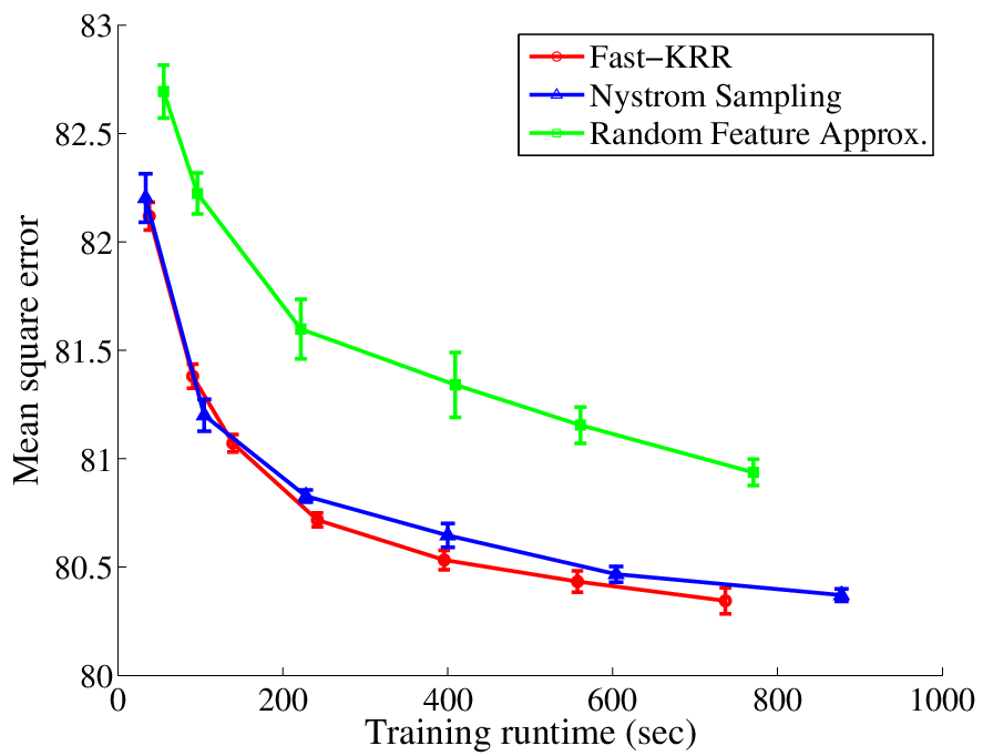
Figure 3: Results on year prediction on held-out test songs for Fast-KRR, Nyström sampling, and random feature approximation. Error bars indicate standard deviations over ten experiments.

We now turn to the results of experiments studying the performance of Fast-KRR on the task of predicting the year in which a song was released based on audio features associated with the song. We use the Million Song Dataset [4], which consists of 463,715 training examples and a second set of 51,630 testing examples. Each example is a song (track) released between 1922 and 2011, and the song is represented as a vector of timbre information computed about the song. Each sample consists of the pair (xi,yi)∈ℝd×ℝ(x_{i},y_{i})\in\mathbb{R}^{d}\times\mathbb{R}, where xi∈ℝdx_{i}\in\mathbb{R}^{d} is a d=90d=90-dimensional vector and yi∈[1922,2011]y_{i}\in[1922,2011] is the year in which the song was released. (For further details, see the paper [4]).

Our experiments with this dataset use the Gaussian radial basis kernel

K⁡(x,x′)=exp⁡(−‖x−x′‖222​σ2).\displaystyle K(x,x^{\prime})=\exp\left(-\frac{\left\|{x-x^{\prime}}\right\|_{2}^{2}}{2\sigma^{2}}\right). (35)

We normalize the feature vectors xx so that the timbre signals have standard deviation 11, and select the bandwidth parameter σ=6\sigma=6 via cross-validation. For regularization, we set λ=N−1\lambda=N^{-1}; since the Gaussian kernel has exponentially decaying eigenvalues (for typical distributions on XX), Corollary 3 shows that this regularization achieves the optimal rate of convergence for the Hilbert space.

In Figure 3, we compare the time-accuracy curve of Fast-KRR with two modern approximation-based methods, plotting the mean-squared error between the predicted release year and the actual year on test songs. The first baseline algorithm is Nyström subsampling [33], where the kernel matrix is approximated by a low-rank matrix of rank D∈{1000,2000,3000,4000,5000,6000}D\in\{1000,2000,3000,4000,5000,6000\}. The second baseline approach is an approximate form of kernel ridge regression using random features [21]. The algorithm approximates the Gaussian kernel (35) by the inner product of two random feature vectors of dimensions D∈{2000,3000,5000,7000,8500,10000}D\in\{2000,3000,5000,7000,8500,10000\}, and then solves the resulting linear regression problem. For the Fast-KRR algorithm, we use seven partitions m∈{32,38,48,64,96,128,256}m\in\{32,38,48,64,96,128,256\} to test the algorithm. Each algorithm is executed 10 times to obtain standard deviations (plotted as error-bars in Figure 3).

As we see in Figure 3, for a fixed time budget, Fast-KRR enjoys the best performance, though the margin between Fast-KRR and Nyström sampling is not substantial. In spite of this close performance between Nyström sampling and the divide-and-conquer Fast-KRR algorithm, it is worth noting that with parallel computation, it is trivial to accelerate Fast-KRR mm times; parallelizing approximation-based methods appears to be a non-trivial task. Moreover, as our results in Section 3 indicate, Fast-KRR is minimax optimal in many regimes. At the same time the conference version of this paper was submitted, Bach [1] published the first results we know of establishing convergence results in ℓ2\ell_{2}-error for Nyström sampling; see the discussion for more detail. We note in passing that standard linear regression with the original 90 features, while quite fast with runtime on the order of 1 second (ignoring data loading), has mean-squared-error 90.4490.44, which is significantly worse than the kernel-based methods.

Refer to caption
Figure 4: Comparison of the performance of Fast-KRR to a standard KRR estimator using a fraction 1/m1/m of the data.

Our final experiment provides a sanity check: is the final averaging step in Fast-KRR even necessary? To this end, we compare Fast-KRR with standard KRR using a fraction 1/m1/m of the data. For the latter approach, we employ the standard regularization λ≈(N/m)−1\lambda\approx(N/m)^{-1}. As Figure 4 shows, Fast-KRR achieves much lower error rates than KRR using only a fraction of the data. Moreover, averaging stabilizes the estimators: the standard deviations of the performance of Fast-KRR are negligible compared to those for standard KRR.

7 Discussion

In this paper, we present results establishing that our decomposition-based algorithm for kernel ridge regression achieves minimax optimal convergence rates whenever the number of splits mm of the data is not too large. The error guarantees of our method depend on the effective dimensionality γ⁡(λ)=∑j=1∞μj/(μj+λ)\gamma(\lambda)=\sum_{j=1}^{\infty}\mu_{j}/(\mu_{j}+\lambda) of the kernel. For any number of splits m≲N/γ​(λ)2m\lesssim N/\gamma(\lambda)^{2}, our method achieves estimation error decreasing as

𝔼⁡[‖f¯−f∗‖22]≲λ​‖f∗‖ℋ2+σ2​γ​(λ)N.\mathbb{E}\left[\|{\bar{f}-f^{*}}\|_{2}^{2}\right]\lesssim\lambda\left\|{f^{*}}\right\|_{\mathcal{H}}^{2}+\frac{\sigma^{2}\gamma(\lambda)}{N}.

(In particular, recall the bound (8) following Theorem 1). Notably, this convergence rate is minimax optimal, and we achieve substantial computational benefits from the subsampling schemes, in that computational cost scales (nearly) linearly in NN.

It is also interesting to consider the number of kernel evaluations required to implement our method. Our estimator requires mm sub-matrices of the full kernel (Gram) matrix, each of size N/m×N/mN/m\times N/m. Since the method may use m≍N/γ2​(λ)m\asymp N/\gamma^{2}(\lambda) machines, in the best case, it requires at most N​γ2​(λ)N\gamma^{2}(\lambda) kernel evaluations. By contrast, Bach [1] shows that Nyström-based subsampling can be used to form an estimator within a constant factor of optimal as long as the number of NN-dimensional subsampled columns of the kernel matrix scales roughly as the marginal dimension γ~​(λ)=N​‖diag(K​(K+λ​N​I)−1)‖∞\widetilde{\gamma}(\lambda)=N\left\|{\mathop{\rm diag}(K(K+\lambda NI)^{-1})}\right\|_{\infty}. Consequently, using roughly N​γ~​(λ)N\widetilde{\gamma}(\lambda) kernel evaluations, Nyström subsampling can achieve optimal convergence rates. These two scalings–namely, N​γ2​(λ)N\gamma^{2}(\lambda) versus N​γ~​(λ)N\widetilde{\gamma}(\lambda)—are currently not comparable: in some situations, such as when the data is not compactly supported, γ~​(λ)\widetilde{\gamma}(\lambda) can scale linearly with NN, while in others it appears to scale roughly as the true effective dimensionality γ⁡(λ)\gamma(\lambda). A natural question arising from these lines of work is to understand the true optimal scaling for these different estimators: is one fundamentally better than the other? Are there natural computational tradeoffs that can be leveraged at large scale? As datasets grow substantially larger and more complex, these questions should become even more important, and we hope to continue to study them.

Acknowledgements:

We thank Francis Bach for interesting and enlightening conversations on the connections between this work and his paper [1] and Yining Wang for pointing out a mistake in an earlier version of this manuscript. JCD was supported by a National Defense Science and Engineering Graduate Fellowship (NDSEG) and a Facebook PhD fellowship. This work was partially supported by ONR MURI grant N00014-11-1-0688 to MJW.

Appendix A Proof of Lemma 1

f^\widehat{f} Empirical KRR minimizer based on nn samples
f∗f^{*} Optimal function generating data, where yi=f∗​(xi)+εiy_{i}=f^{*}(x_{i})+\varepsilon_{i}
Δ\Delta Error f^−f∗\widehat{f}-f^{*}
ξx\xi_{x} RKHS evaluator ξx:=K⁡(x,⋅)\xi_{x}:=K(x,\cdot), so ⟨f,ξx⟩=⟨ξx,f⟩=f⁡(x)\left\langle f,\xi_{x}\right\rangle=\left\langle\xi_{x},f\right\rangle=f(x)
Σ^\widehat{\Sigma} Operator mapping ℋ→ℋ\mathcal{H}\rightarrow\mathcal{H} defined as the outer product Σ^:=1n​∑i=1nξxi⊗ξxi\widehat{\Sigma}:=\frac{1}{n}\sum_{i=1}^{n}\xi_{x_{i}}\otimes\xi_{x_{i}}, so that Σ^​f=1n​∑i=1n⟨ξxi,f⟩​ξxi\widehat{\Sigma}f=\frac{1}{n}\sum_{i=1}^{n}\left\langle\xi_{x_{i}},f\right\rangle\xi_{x_{i}}
ϕj\phi_{j} jjth orthonormal basis vector for L2​(ℙ)L^{2}(\mathbb{P})
δj\delta_{j} Basis coefficients of Δ\Delta or 𝔼⁡[Δ∣X]\mathbb{E}[\Delta\mid X] (depending on context), i.e. Δ=∑j=1∞δj​ϕj\Delta=\sum_{j=1}^{\infty}\delta_{j}\phi_{j}
θj\theta_{j} Basis coefficients of f∗f^{*}, i.e. f∗=∑j=1∞θj​ϕjf^{*}=\sum_{j=1}^{\infty}\theta_{j}\phi_{j}
dd Integer-valued truncation point
MM Diagonal matrix with M=diag(μ1,…,μd)M=\mathop{\rm diag}(\mu_{1},\ldots,\mu_{d})
QQ Diagonal matrix with Q=(Id×d+λ​M−1)12Q=(I_{d\times d}+\lambda M^{-1})^{\frac{1}{2}}
Φ\Phi n×dn\times d matrix with coordinates Φi​j=ϕj​(xi)\Phi_{ij}=\phi_{j}(x_{i})
v↓{v}^{\downarrow} Truncation of vector vv. For v=∑jνj​ϕj∈ℋv=\sum_{j}\nu_{j}\phi_{j}\in\mathcal{H}, defined as v↓=∑j=1dνj​ϕj{v}^{\downarrow}=\sum_{j=1}^{d}\nu_{j}\phi_{j}; for v∈ℓ2​(ℕ)v\in\ell_{2}(\mathbb{N}) defined as v↓=(v1,…,vd){v}^{\downarrow}=(v_{1},\ldots,v_{d})
v↑{v}^{\uparrow} Untruncated part of vector vv, defined as v↑=(vd+1,vd+1,…){v}^{\uparrow}=(v_{d+1},v_{d+1},\ldots)
βd\beta_{d} The tail sum ∑j>dμj\sum_{j>d}\mu_{j}
γ⁡(λ)\gamma(\lambda) The sum ∑j=1∞1/(1+λ/μj)\sum_{j=1}^{\infty}1/(1+\lambda/\mu_{j})
b⁡(n,d,k)b(n,d,k) The maximum max⁡{max⁡{k,log⁡(d)},max⁡{k,log⁡(d)}/n1/2−1/k}\max\{\sqrt{\max\{k,\log(d)\}},\max\{k,\log(d)\}/n^{1/2-1/k}\}
Table 2: Notation used in proofs

This appendix is devoted to the bias bound stated in Lemma 1. Let X={xi}i=1nX=\{x_{i}\}_{i=1}^{n} be shorthand for the design matrix, and define the error vector Δ=f^−f∗\Delta=\widehat{f}-f^{*}. By Jensen’s inequality, we have ‖𝔼⁡[Δ]‖2≤𝔼⁡[‖𝔼⁡[Δ∣X]‖2]\left\|{\mathbb{E}[\Delta]}\right\|_{2}\leq\mathbb{E}[\left\|{\mathbb{E}[\Delta\mid X]}\right\|_{2}], so it suffices to provide a bound on ‖𝔼⁡[Δ∣X]‖2\left\|{\mathbb{E}[\Delta\mid X]}\right\|_{2}. Throughout this proof and the remainder of the paper, we represent the kernel evaluator by the function ξx\xi_{x}, where ξx:=K⁡(x,⋅)\xi_{x}:=K(x,\cdot) and f⁡(x)=⟨ξx,f⟩f(x)=\left\langle\xi_{x},f\right\rangle for any f∈ℋf\in\mathcal{H}. Using this notation, the estimate f^\widehat{f} minimizes the empirical objective

1n​∑i=1n(⟨ξxi,f⟩ℋ−yi)2+λ​‖f‖ℋ2.\frac{1}{n}\sum_{i=1}^{n}\left(\left\langle\xi_{x_{i}},f\right\rangle_{\mathcal{H}}-y_{i}\right)^{2}+\lambda\left\|{f}\right\|_{\mathcal{H}}^{2}. (36)

This objective is Fréchet differentiable, and as a consequence, the necessary and sufficient conditions for optimality [18] of f^\widehat{f} are that

1n​∑i=1n(⟨ξxi,f^−f∗⟩ℋ−εi)+λ​f^=1n​∑i=1n(⟨ξxi,f^⟩ℋ−yi)+λ​f^=0.\frac{1}{n}\sum_{i=1}^{n}(\langle\xi_{x_{i}},\widehat{f}-f^{*}\rangle_{\mathcal{H}}-\varepsilon_{i})+\lambda\widehat{f}=\frac{1}{n}\sum_{i=1}^{n}(\langle\xi_{x_{i}},\widehat{f}\rangle_{\mathcal{H}}-y_{i})+\lambda\widehat{f}=0. (37)

Taking conditional expectations over the noise variables {εi}i=1n\{\varepsilon_{i}\}_{i=1}^{n} with the design X={xi}i=1nX=\{x_{i}\}_{i=1}^{n} fixed, we find that

1n​∑i=1nξxi​⟨ξxi,𝔼⁡[Δ∣X]⟩+λ​𝔼​[f^∣X]=0.\frac{1}{n}\sum_{i=1}^{n}\xi_{x_{i}}\left\langle\xi_{x_{i}},\mathbb{E}[\Delta\mid X]\right\rangle+\lambda\mathbb{E}[\widehat{f}\mid X]=0.

Define the sample covariance operator Σ^:=1n​∑i=1nξxi⊗ξxi\widehat{\Sigma}:=\frac{1}{n}\sum_{i=1}^{n}\xi_{x_{i}}\otimes\xi_{x_{i}}. Adding and subtracting λ​f∗\lambda f^{*} from the above equation yields

(Σ^+λ​I)​𝔼​[Δ∣X]\displaystyle(\widehat{\Sigma}+\lambda I)\mathbb{E}[\Delta\mid X] =−λ​f∗.\displaystyle=-\lambda f^{*}. (38)

Consequently, we see we have ‖𝔼⁡[Δ∣X]‖ℋ≤‖f∗‖ℋ\left\|{\mathbb{E}[\Delta\mid X]}\right\|_{\mathcal{H}}\leq\left\|{f^{*}}\right\|_{\mathcal{H}}, since Σ^⪰0\widehat{\Sigma}\succeq 0.

We now use a truncation argument to reduce the problem to a finite dimensional problem. To do so, we let δ∈ℓ2​(ℕ)\delta\in\ell_{2}(\mathbb{N}) denote the coefficients of 𝔼⁡[Δ∣X]\mathbb{E}[\Delta\mid X] when expanded in the basis {ϕj}j=1∞\{\phi_{j}\}_{j=1}^{\infty}:

𝔼⁡[Δ∣X]\displaystyle\mathbb{E}[\Delta\mid X] =∑j=1∞δj​ϕj,with δj=⟨𝔼⁡[Δ∣X],ϕj⟩L2​(ℙ).\displaystyle=\sum_{j=1}^{\infty}\delta_{j}\phi_{j},\quad\mbox{with $\delta_{j}=\left\langle{\mathbb{E}[\Delta\mid X]},{\phi_{j}}\right\rangle_{L^{2}(\mathbb{P})}$.} (39)

For a fixed d∈ℕd\in\mathbb{N}, define the vectors δ↓:=(δ1,…,δd){\delta}^{\downarrow}:=(\delta_{1},\ldots,\delta_{d}) and δ↑:=(δd+1,δd+2,…){\delta}^{\uparrow}:=(\delta_{d+1},\delta_{d+2},\ldots) (we suppress dependence on dd for convenience). By the orthonormality of the collection {ϕj}\{\phi_{j}\}, we have

‖𝔼⁡[Δ∣X]‖22\displaystyle\left\|{\mathbb{E}[\Delta\mid X]}\right\|_{2}^{2} =‖δ‖22=‖δ↓‖22+‖δ↑‖22.\displaystyle=\left\|{\delta}\right\|_{2}^{2}=\|{{\delta}^{\downarrow}}\|_{2}^{2}+\|{{\delta}^{\uparrow}}\|_{2}^{2}. (40)

We control each of the elements of the sum (40) in turn.

Control of the term ‖δ↑‖22\|{{\delta}^{\uparrow}}\|_{2}^{2}:

By definition, we have

‖δ↑‖22=μd+1μd+1​∑j=d+1∞δj2\displaystyle\|{{\delta}^{\uparrow}}\|_{2}^{2}=\frac{\mu_{d+1}}{\mu_{d+1}}\sum_{j=d+1}^{\infty}\delta_{j}^{2} ≤μd+1​∑j=d+1∞δj2μj≤(i)μd+1​‖𝔼⁡[Δ∣X]‖ℋ2(i​i)≤μd+1​‖f∗‖ℋ2,\displaystyle\,\leq\,\mu_{d+1}\sum_{j=d+1}^{\infty}\frac{\delta_{j}^{2}}{\mu_{j}}\,\stackrel{{\scriptstyle(i)}}{{\leq}}\,\mu_{d+1}\left\|{\mathbb{E}[\Delta\mid X]}\right\|_{\mathcal{H}}^{2}\,\stackrel{{\scriptstyle(ii)}}{{\,}}\leq\mu_{d+1}\left\|{f^{*}}\right\|_{\mathcal{H}}^{2}, (41)

where inequality (i) follows since ‖𝔼⁡[Δ∣X]‖ℋ2=∑j=1∞δj2μj\left\|{\mathbb{E}[\Delta\mid X]}\right\|_{\mathcal{H}}^{2}=\sum_{j=1}^{\infty}\frac{\delta_{j}^{2}}{\mu_{j}}; and inequality (ii) follows from the bound ‖𝔼⁡[Δ∣X]‖ℋ≤‖f∗‖ℋ\left\|{\mathbb{E}[\Delta\mid X]}\right\|_{\mathcal{H}}\leq\left\|{f^{*}}\right\|_{\mathcal{H}}, which is a consequence of equality (38).

Control of the term ‖δ↓‖22\|{{\delta}^{\downarrow}}\|_{2}^{2}:

Let (θ1,θ2,…)(\theta_{1},\theta_{2},\ldots) be the coefficients of f∗f^{*} in the basis {ϕj}\{\phi_{j}\}. In addition, define the matrices Φ∈ℝn×d\Phi\in\mathbb{R}^{n\times d} by

Φi​j=ϕj​(xi)​for ​i∈{1,…,n}, and ​j∈{1,…,d}\Phi_{ij}=\phi_{j}(x_{i})~~\mbox{for~}i\in\{1,\ldots,n\},\mbox{ and }j\in\{1,\ldots,d\}

and M=diag(μ1,…,μd)≻0∈ℝd×dM=\mathop{\rm diag}(\mu_{1},\ldots,\mu_{d})\succ 0\in\mathbb{R}^{d\times d}. Lastly, define the tail error vector v∈ℝnv\in\mathbb{R}^{n} by

vi\displaystyle v_{i} :=∑j>dδj​ϕj​(xi)=𝔼⁡[Δ↑​(xi)∣X].\displaystyle:\,=\sum_{j>d}\delta_{j}\phi_{j}(x_{i})=\mathbb{E}[{\Delta}^{\uparrow}(x_{i})\mid X].

Let l∈ℕl\in\mathbb{N} be arbitrary. Computing the (Hilbert) inner product of the terms in equation (38) with ϕl\phi_{l}, we obtain

−λ​θlμl=⟨ϕl,−λ​f∗⟩=⟨ϕl,(Σ^+λ)​𝔼​[Δ∣X]⟩\displaystyle-\lambda\frac{\theta_{l}}{\mu_{l}}=\left\langle\phi_{l},-\lambda f^{*}\right\rangle=\left\langle\phi_{l},(\widehat{\Sigma}+\lambda)\mathbb{E}[\Delta\mid X]\right\rangle
=1n​∑i=1n⟨ϕl,ξxi⟩​⟨ξxi,𝔼⁡[Δ∣X]⟩+λ⁡⟨ϕl,𝔼⁡[Δ∣X]⟩=1n​∑i=1nϕl​(xi)​𝔼​[Δ⁡(xi)∣X]+λ​δlμl.\displaystyle\quad=\frac{1}{n}\sum_{i=1}^{n}\left\langle\phi_{l},\xi_{x_{i}}\right\rangle\left\langle\xi_{x_{i}},\mathbb{E}[\Delta\mid X]\right\rangle+\lambda\left\langle\phi_{l},\mathbb{E}[\Delta\mid X]\right\rangle=\frac{1}{n}\sum_{i=1}^{n}\phi_{l}(x_{i})\mathbb{E}[\Delta(x_{i})\mid X]+\lambda\frac{\delta_{l}}{\mu_{l}}.

We can rewrite the final sum above using the fact that Δ=Δ↓+Δ↑\Delta={\Delta}^{\downarrow}+{\Delta}^{\uparrow}, which implies

1n​∑i=1nϕl​(xi)​𝔼​[Δ⁡(xi)∣X]=1n​∑i=1nϕl​(xi)​(∑j=1dϕj​(xi)​δj+∑j>dϕj​(xi)​δj)\frac{1}{n}\sum_{i=1}^{n}\phi_{l}(x_{i})\mathbb{E}[\Delta(x_{i})\mid X]=\frac{1}{n}\sum_{i=1}^{n}\phi_{l}(x_{i})\bigg(\sum_{j=1}^{d}\phi_{j}(x_{i})\delta_{j}+\sum_{j>d}\phi_{j}(x_{i})\delta_{j}\bigg)

Applying this equality for l=1,2,…,dl=1,2,\ldots,d yields

(1n​ΦT​Φ+λ​M−1)​δ↓=−λ​M−1​θ↓−1n​ΦT​v.\left(\frac{1}{n}\Phi^{T}\Phi+\lambda M^{-1}\right){\delta}^{\downarrow}=-\lambda M^{-1}{\theta}^{\downarrow}-\frac{1}{n}\Phi^{T}v. (42)

We now show how the expression (42) gives us the desired bound in the lemma. By definining the shorthand matrix Q=(I+λ​M−1)1/2Q=(I+\lambda M^{-1})^{1/2}, we have

1n​ΦT​Φ+λ​M−1=I+λ​M−1+1n​ΦT​Φ−I=Q⁡(I+Q−1​(1n​ΦT​Φ−I)​Q−1)​Q.\frac{1}{n}\Phi^{T}\Phi+\lambda M^{-1}=I+\lambda M^{-1}+\frac{1}{n}\Phi^{T}\Phi-I=Q\left(I+Q^{-1}\left(\frac{1}{n}\Phi^{T}\Phi-I\right)Q^{-1}\right)Q.

As a consequence, we can rewrite expression (42) to

(I+Q−1​(1n​ΦT​Φ−I)​Q−1)​Q​δ↓=−λ​Q−1​M−1​θ↓−1n​Q−1​ΦT​v.\left(I+Q^{-1}\left(\frac{1}{n}\Phi^{T}\Phi-I\right)Q^{-1}\right)Q{\delta}^{\downarrow}=-\lambda Q^{-1}M^{-1}{\theta}^{\downarrow}-\frac{1}{n}Q^{-1}\Phi^{T}v. (43)

We now present a lemma bounding the terms in equality (43) to control δ↓{\delta}^{\downarrow}.

Lemma 5

The following bounds hold:

‖λ​Q−1​M−1​θ↓‖22≤λ​‖f∗‖ℋ2,and\displaystyle\left\|{\lambda Q^{-1}M^{-1}{\theta}^{\downarrow}}\right\|_{2}^{2}\leq\lambda\left\|{f^{*}}\right\|_{\mathcal{H}}^{2},\quad\mbox{and} (44a)
𝔼⁡[‖1n​Q−1​ΦT​v‖22]≤ρ4​‖f∗‖ℋ2​tr(K)​βdλ.\displaystyle\mathbb{E}\left[\left\|{\frac{1}{n}Q^{-1}\Phi^{T}v}\right\|_{2}^{2}\right]\leq\frac{\rho^{4}\left\|{f^{*}}\right\|_{\mathcal{H}}^{2}\mathop{\rm tr}(K)\beta_{d}}{\lambda}. (44b)

Define the event ℰ:={|||Q−1(1nΦTΦ−I)Q−1|||≤1/2}\mathcal{E}:=\left\{\left|\!\left|\!\left|{Q^{-1}\left(\frac{1}{n}\Phi^{T}\Phi-I\right)Q^{-1}}\right|\!\right|\!\right|\leq 1/2\right\}. Under Assumption A with moment bound 𝔼⁡[ϕj​(X)2​k]≤ρ2​k\mathbb{E}[\phi_{j}(X)^{2k}]\leq\rho^{2k}, there exists a universal constant CC such that

ℙ⁡(ℰc)≤(max⁡{k∨log⁡(d),k∨log⁡(d)n1/2−1/k}​C​ρ2​γ​(λ)n)k.\mathbb{P}(\mathcal{E}^{c})\leq\left(\max\left\{\sqrt{k\vee\log(d)},\frac{k\vee\log(d)}{n^{1/2-1/k}}\right\}\frac{C\rho^{2}\gamma(\lambda)}{\sqrt{n}}\right)^{k}. (45)

We defer the proof of this lemma to Appendix A.1.

Based on this lemma, we can now complete the proof. Whenever the event ℰ\mathcal{E} holds, we know that I+Q−1​((1/n)​ΦT​Φ−I)​Q−1⪰(1/2)​II+Q^{-1}((1/n)\Phi^{T}\Phi-I)Q^{-1}\succeq(1/2)I. In particular, we have

‖Q​δ↓‖22≤4​‖λ​Q−1​M−1​θ↓+(1/n)​Q−1​ΦT​v‖22\|{{Q\delta}^{\downarrow}}\|_{2}^{2}\leq 4\left\|{\lambda Q^{-1}M^{-1}{\theta}^{\downarrow}+(1/n)Q^{-1}\Phi^{T}v}\right\|_{2}^{2}

on ℰ\mathcal{E}, by Eq. (43). Since ‖Q​δ↓‖22≥‖δ↓‖22\|{{Q\delta}^{\downarrow}}\|_{2}^{2}\geq\|{{\delta}^{\downarrow}}\|_{2}^{2}, the above inequality implies that

‖δ↓‖22≤4​‖λ​Q−1​M−1​θ↓+(1/n)​Q−1​ΦT​v‖22\|{{\delta}^{\downarrow}}\|_{2}^{2}\leq 4\left\|{\lambda Q^{-1}M^{-1}{\theta}^{\downarrow}+(1/n)Q^{-1}\Phi^{T}v}\right\|_{2}^{2}

Since ℰ\mathcal{E} is XX-measureable, we thus obtain

𝔼⁡[‖δ↓‖22]\displaystyle\mathbb{E}\left[\|{{\delta}^{\downarrow}}\|_{2}^{2}\right] =𝔼⁡[(ℰ)​‖δ↓‖22]+𝔼⁡[(ℰc)​‖δ↓‖22]\displaystyle=\mathbb{E}\left[1\!\left({\mathcal{E}}\right)\|{{\delta}^{\downarrow}}\|_{2}^{2}\right]+\mathbb{E}\left[1\!\left({\mathcal{E}^{c}}\right)\|{{\delta}^{\downarrow}}\|_{2}^{2}\right]
≤4​𝔼​[(ℰ)​‖λ​Q−1​M−1​θ↓+(1/n)​Q−1​ΦT​v‖22]+𝔼⁡[(ℰc)​‖δ↓‖22].\displaystyle\leq 4\mathbb{E}\left[1\!\left({\mathcal{E}}\right)\left\|{\lambda Q^{-1}M^{-1}{\theta}^{\downarrow}+(1/n)Q^{-1}\Phi^{T}v}\right\|_{2}^{2}\right]+\mathbb{E}\left[1\!\left({\mathcal{E}^{c}}\right)\|{{\delta}^{\downarrow}}\|_{2}^{2}\right].

Applying the bounds (44a) and (44b), along with the elementary inequality (a+b)2≤2​a2+2​b2(a+b)^{2}\leq 2a^{2}+2b^{2}, we have

𝔼⁡[‖δ↓‖22]≤8​λ​‖f∗‖ℋ2+8​ρ4​‖f∗‖ℋ2​tr(K)​βdλ+𝔼⁡[(ℰc)​‖δ↓‖22].\mathbb{E}\left[\|{{\delta}^{\downarrow}}\|_{2}^{2}\right]\leq 8\lambda\left\|{f^{*}}\right\|_{\mathcal{H}}^{2}+\frac{8\rho^{4}\left\|{f^{*}}\right\|_{\mathcal{H}}^{2}\mathop{\rm tr}(K)\beta_{d}}{\lambda}+\mathbb{E}\left[1\!\left({\mathcal{E}^{c}}\right)\|{{\delta}^{\downarrow}}\|_{2}^{2}\right]. (46)

Now we use the fact that by the gradient optimality condition (38), ‖𝔼⁡[Δ∣X]‖22≤‖f∗‖22\left\|{\mathbb{E}[\Delta\mid X]}\right\|_{2}^{2}\leq\left\|{f^{*}}\right\|_{2}^{2}. Recalling the shorthand (6) for b⁡(n,d,k)b(n,d,k), we apply the bound (45) to see

𝔼⁡[(ℰc)​‖δ↓‖22]≤ℙ⁡(ℰc)​‖f∗‖22≤(C​b​(n,d,k)​ρ2​γ​(λ)n)k​‖f∗‖22.\mathbb{E}\left[1\!\left({\mathcal{E}^{c}}\right)\|{{\delta}^{\downarrow}}\|_{2}^{2}\right]\leq\mathbb{P}(\mathcal{E}^{c})\left\|{f^{*}}\right\|_{2}^{2}\leq\left(\frac{Cb(n,d,k)\rho^{2}\gamma(\lambda)}{\sqrt{n}}\right)^{k}\left\|{f^{*}}\right\|_{2}^{2}.

Combining this with the inequality (46), we obtain the desired statement of Lemma 1.

A.1 Proof of Lemma 5

Proof of bound (44a):

Beginning with the proof of the bound (44a), we have

‖Q−1​M−1​θ↓‖22\displaystyle\left\|{Q^{-1}M^{-1}{\theta}^{\downarrow}}\right\|_{2}^{2} =(θ↓)T​(M2+λ​M)−1​θ↓\displaystyle=({\theta}^{\downarrow})^{T}(M^{2}+\lambda M)^{-1}{\theta}^{\downarrow}
≤(θ↓)T​(λ​M)−1​θ↓=1λ​(θ↓)T​M−1​θ↓≤1λ​‖f∗‖ℋ2.\displaystyle\leq({\theta}^{\downarrow})^{T}(\lambda M)^{-1}{\theta}^{\downarrow}=\frac{1}{\lambda}({\theta}^{\downarrow})^{T}M^{-1}{\theta}^{\downarrow}\leq\frac{1}{\lambda}\left\|{f^{*}}\right\|_{\mathcal{H}}^{2}.

Multiplying both sides by λ2\lambda^{2} gives the result.

Proof of bound (44b):

Next we turn to the proof of the bound (44b). We begin by re-writing Q−1​ΦT​vQ^{-1}\Phi^{T}v as the product of two components:

1nQ−1ΦTv=(M+λI)−1/2(1nM1/2ΦTv).\frac{1}{n}Q^{-1}\Phi^{T}v=(M+\lambda I)^{-1/2}\left(\frac{1}{n}M^{1/2}\Phi^{T}v\right). (47)

The first matrix is a diagonal matrix whose operator norm is bounded:

|||(M+λI)−1/2|||=maxj∈[d]1μj+λ≤1λ.\left|\!\left|\!\left|{(M+\lambda I)^{-1/2}}\right|\!\right|\!\right|=\max_{j\in[d]}\frac{1}{\sqrt{\mu_{j}+\lambda}}\leq\frac{1}{\sqrt{\lambda}}. (48)

For the second factor in the product (47), the analysis is a little more complicated. Let Φℓ=(ϕl​(x1),…,ϕl​(xn))\Phi_{\ell}=(\phi_{l}(x_{1}),\ldots,\phi_{l}(x_{n})) be the ℓ\ellth column of Φ\Phi. In this case,

‖M1/2​ΦT​v‖22\displaystyle\left\|{M^{1/2}\Phi^{T}v}\right\|_{2}^{2} =∑ℓ=1dμℓ​(ΦℓT​v)2≤∑ℓ=1dμℓ​‖Φℓ‖22​‖v‖22,\displaystyle=\sum_{\ell=1}^{d}\mu_{\ell}(\Phi_{\ell}^{T}v)^{2}\leq\sum_{\ell=1}^{d}\mu_{\ell}\left\|{\Phi_{\ell}}\right\|_{2}^{2}\left\|{v}\right\|_{2}^{2}, (49)

using the Cauchy-Schwarz inequality. Taking expectations with respect to the design {xi}i=1n\{x_{i}\}_{i=1}^{n} and applying Hölder’s inequality yields

𝔼⁡[‖Φℓ‖22​‖v‖22]≤𝔼⁡[‖Φℓ‖24]​𝔼⁡[‖v‖24].\mathbb{E}[\left\|{\Phi_{\ell}}\right\|_{2}^{2}\left\|{v}\right\|_{2}^{2}]\leq\sqrt{\mathbb{E}[\left\|{\Phi_{\ell}}\right\|_{2}^{4}]}\sqrt{\mathbb{E}[\left\|{v}\right\|_{2}^{4}]}.

We bound each of the terms in this product in turn. For the first, we have

𝔼⁡[‖Φℓ‖24]\displaystyle\mathbb{E}[\left\|{\Phi_{\ell}}\right\|_{2}^{4}] =𝔼⁡[(∑i=1nϕℓ2​(Xi))2]=𝔼⁡[∑i,j=1nϕℓ2​(Xi)​ϕℓ2​(Xj)]≤n2​𝔼​[ϕℓ4​(X1)]≤n2​ρ4\displaystyle=\mathbb{E}\bigg[\bigg(\sum_{i=1}^{n}\phi_{\ell}^{2}(X_{i})\bigg)^{2}\bigg]=\mathbb{E}\bigg[\sum_{i,j=1}^{n}\phi_{\ell}^{2}(X_{i})\phi_{\ell}^{2}(X_{j})\bigg]\leq n^{2}\mathbb{E}[\phi_{\ell}^{4}(X_{1})]\leq n^{2}\rho^{4}

since the XiX_{i} are i.i.d., 𝔼⁡[ϕℓ2​(X1)]≤𝔼⁡[ϕℓ4​(X1)]\mathbb{E}[\phi_{\ell}^{2}(X_{1})]\leq\sqrt{\mathbb{E}[\phi_{\ell}^{4}(X_{1})]}, and 𝔼⁡[ϕℓ4​(X1)]≤ρ4\mathbb{E}[\phi_{\ell}^{4}(X_{1})]\leq\rho^{4} by assumption. Turning to the term involving vv, we have

vi2=(∑j>dδj​ϕj​(xi))2≤(∑j>dδj2μj)​(∑j>dμj​ϕj2​(xi))v_{i}^{2}=\bigg(\sum_{j>d}\delta_{j}\phi_{j}(x_{i})\bigg)^{2}\leq\bigg(\sum_{j>d}\frac{\delta_{j}^{2}}{\mu_{j}}\bigg)\bigg(\sum_{j>d}\mu_{j}\phi_{j}^{2}(x_{i})\bigg)

by Cauchy-Schwarz. As a consequence, we find

𝔼⁡[‖v‖24]=𝔼⁡[(n​1n​∑i=1nvi2)2]≤n2​1n​∑i=1n𝔼⁡[vi4]\displaystyle\mathbb{E}[\left\|{v}\right\|_{2}^{4}]=\mathbb{E}\bigg[\bigg(n\frac{1}{n}\sum_{i=1}^{n}v_{i}^{2}\bigg)^{2}\bigg]\leq n^{2}\frac{1}{n}\sum_{i=1}^{n}\mathbb{E}[v_{i}^{4}] ≤n​∑i=1n𝔼⁡[(∑j>dδj2μj)2​(∑j>dμj​ϕj2​(Xi))2]\displaystyle\leq n\sum_{i=1}^{n}\mathbb{E}\bigg[\bigg(\sum_{j>d}\frac{\delta_{j}^{2}}{\mu_{j}}\bigg)^{2}\bigg(\sum_{j>d}\mu_{j}\phi_{j}^{2}(X_{i})\bigg)^{2}\bigg]
≤n2​𝔼​[‖𝔼⁡[Δ∣X]‖ℋ4​(∑j>dμj​ϕj2​(X1))2],\displaystyle\leq n^{2}\mathbb{E}\bigg[\left\|{\mathbb{E}[\Delta\mid X]}\right\|_{\mathcal{H}}^{4}\bigg(\sum_{j>d}\mu_{j}\phi_{j}^{2}(X_{1})\bigg)^{2}\bigg],

since the XiX_{i} are i.i.d. Using the fact that ‖𝔼⁡[Δ∣X]‖ℋ≤‖f∗‖ℋ\left\|{\mathbb{E}[\Delta\mid X]}\right\|_{\mathcal{H}}\leq\left\|{f^{*}}\right\|_{\mathcal{H}}, we expand the second square to find

1n2​𝔼​[‖v‖24]≤‖f∗‖ℋ4​∑j,k>d𝔼⁡[μj​μk​ϕj2​(X1)​ϕk2​(X1)]≤‖f∗‖ℋ4​ρ4​∑j,k>dμj​μk=‖f∗‖ℋ4​ρ4​(∑j>dμj)2.\frac{1}{n^{2}}\mathbb{E}[\left\|{v}\right\|_{2}^{4}]\leq\left\|{f^{*}}\right\|_{\mathcal{H}}^{4}\sum_{j,k>d}\mathbb{E}\left[\mu_{j}\mu_{k}\phi_{j}^{2}(X_{1})\phi_{k}^{2}(X_{1})\right]\leq\left\|{f^{*}}\right\|_{\mathcal{H}}^{4}\rho^{4}\sum_{j,k>d}\mu_{j}\mu_{k}=\left\|{f^{*}}\right\|_{\mathcal{H}}^{4}\rho^{4}\bigg(\sum_{j>d}\mu_{j}\bigg)^{2}.

Combining our bounds on ‖Φℓ‖2\left\|{\Phi_{\ell}}\right\|_{2} and ‖v‖2\left\|{v}\right\|_{2} with our initial bound (49), we obtain the inequality

𝔼⁡[‖M1/2​ΦT​v‖22]≤∑l=1dμℓ​n2​ρ4​n2​‖f∗‖ℋ4​ρ4​(∑j>dμj)2=n2​ρ4​‖f∗‖ℋ2​(∑j>dμj)​∑l=1dμℓ.\mathbb{E}\left[\left\|{M^{1/2}\Phi^{T}v}\right\|_{2}^{2}\right]\leq\sum_{l=1}^{d}\mu_{\ell}\sqrt{n^{2}\rho^{4}}\sqrt{n^{2}\left\|{f^{*}}\right\|_{\mathcal{H}}^{4}\rho^{4}\bigg(\sum_{j>d}\mu_{j}\bigg)^{2}}=n^{2}\rho^{4}\left\|{f^{*}}\right\|_{\mathcal{H}}^{2}\bigg(\sum_{j>d}\mu_{j}\bigg)\sum_{l=1}^{d}\mu_{\ell}.

Dividing by n2n^{2}, recalling the definition of βd=∑j>dμj\beta_{d}=\sum_{j>d}\mu_{j}, and noting that tr(K)≥∑l=1dμℓ\mathop{\rm tr}(K)\geq\sum_{l=1}^{d}\mu_{\ell} shows that

𝔼⁡[‖1n​M1/2​ΦT​v‖22]≤ρ4​‖f∗‖ℋ2​βd​tr(K).\mathbb{E}\left[\left\|{\frac{1}{n}M^{1/2}\Phi^{T}v}\right\|_{2}^{2}\right]\leq\rho^{4}\left\|{f^{*}}\right\|_{\mathcal{H}}^{2}\beta_{d}\mathop{\rm tr}(K).

Combining this inequality with our expansion (47) and the bound (48) yields the claim (44b).

Proof of bound (45):

Let us consider the expectation of the norm of the matrix Q−1​((1/n)​ΦT​Φ−I)​Q−1Q^{-1}((1/n)\Phi^{T}\Phi-I)Q^{-1}. For each i∈[n]i\in[n], let πi=(ϕ1​(xi),…,ϕd​(xi))∈ℝd\pi_{i}=(\phi_{1}(x_{i}),\ldots,\phi_{d}(x_{i}))\in\mathbb{R}^{d} denote the iith row of the matrix Φ∈ℝn×d\Phi\in\mathbb{R}^{n\times d}. Then we know that

Q−1​(1n​ΦT​Φ−I)​Q−1=1n​∑i=1nQ−1​(πi​πiT−I)​Q−1.Q^{-1}\left(\frac{1}{n}\Phi^{T}\Phi-I\right)Q^{-1}=\frac{1}{n}\sum_{i=1}^{n}Q^{-1}(\pi_{i}\pi_{i}^{T}-I)Q^{-1}.

Define the sequence of matrices

Ai:=Q−1​(πi​πiT−I)​Q−1A_{i}:=Q^{-1}(\pi_{i}\pi_{i}^{T}-I)Q^{-1}

Then the matrices Ai=AiT∈ℝd×dA_{i}=A_{i}^{T}\in\mathbb{R}^{d\times d}. Note that 𝔼⁡[Ai]=0\mathbb{E}[A_{i}]=0 and let εi\varepsilon_{i} be i.i.d. {−1,1}\{-1,1\}-valued Rademacher random variables. Applying a standard symmetrization argument [17], we find that for any k≥1k\geq 1, we have

𝔼⁡[‖|Q−1​(1n​ΦT​Φ−I)​Q−1|‖k]=𝔼⁡[‖|1n​∑i=1nAi|‖k]≤2k​𝔼​[‖|1n​∑i=1nεi​Ai|‖k].\mathbb{E}\left[\left|\!\left|\!\left|{Q^{-1}\left(\frac{1}{n}\Phi^{T}\Phi-I\right)Q^{-1}}\right|\!\right|\!\right|^{k}\right]=\mathbb{E}\left[\left|\!\left|\!\left|{\frac{1}{n}\sum_{i=1}^{n}A_{i}}\right|\!\right|\!\right|^{k}\right]\leq 2^{k}\mathbb{E}\left[\left|\!\left|\!\left|{\frac{1}{n}\sum_{i=1}^{n}\varepsilon_{i}A_{i}}\right|\!\right|\!\right|^{k}\right]. (50)
Lemma 6

The quantity 𝔼​[‖|1n​∑i=1nεi​Ai|‖k]1/k\mathbb{E}\left[\left|\!\left|\!\left|{\frac{1}{n}\sum_{i=1}^{n}\varepsilon_{i}A_{i}}\right|\!\right|\!\right|^{k}\right]^{1/k} is upper bounded by

e⁡(k∨2​log⁡(d))​ρ2​∑j=1d11+λ/μjn+4​e​(k∨2​log⁡(d))n1−1/k​(∑j=1dρ21+λ/μj).\displaystyle\sqrt{e(k\vee 2\log(d))}\frac{\rho^{2}\sum_{j=1}^{d}\frac{1}{1+\lambda/\mu_{j}}}{\sqrt{n}}+\frac{4e(k\vee 2\log(d))}{n^{1-1/k}}\bigg(\sum_{j=1}^{d}\frac{\rho^{2}}{1+\lambda/\mu_{j}}\bigg). (51)

We take this lemma as given for the moment, returning to prove it shortly. Recall the definition of the constant γ⁡(λ)=∑j=1∞1/(1+λ/μj)≥∑j=1d1/(1+λ/μj)\gamma(\lambda)=\sum_{j=1}^{\infty}1/(1+\lambda/\mu_{j})\geq\sum_{j=1}^{d}1/(1+\lambda/\mu_{j}). Then using our symmetrization inequality (50), we have

𝔼⁡[‖|Q−1​(1n​ΦT​Φ−I)​Q−1|‖k]\displaystyle\mathbb{E}\bigg[\left|\!\left|\!\left|{Q^{-1}\left(\frac{1}{n}\Phi^{T}\Phi-I\right)Q^{-1}}\right|\!\right|\!\right|^{k}\bigg]
≤2k​(e⁡(k∨log⁡(d))​ρ2​γ​(λ)n+4​e​(k∨2​log⁡(d))n1−1/k​ρ2​γ​(λ))k\displaystyle\leq 2^{k}\left(\sqrt{e(k\vee\log(d))}\frac{\rho^{2}\gamma(\lambda)}{\sqrt{n}}+\frac{4e(k\vee 2\log(d))}{n^{1-1/k}}\rho^{2}\gamma(\lambda)\right)^{k}
≤max⁡{k∨log⁡(d),k∨log⁡(d)n1/2−1/k}k​(C​ρ2​γ​(λ)n)k,\displaystyle\leq\max\left\{\sqrt{k\vee\log(d)},\frac{k\vee\log(d)}{n^{1/2-1/k}}\right\}^{k}\left(\frac{C\rho^{2}\gamma(\lambda)}{\sqrt{n}}\right)^{k}, (52)

where CC is a numerical constant. By definition of the event ℰ\mathcal{E}, we see by Markov’s inequality that for any k∈ℝ,k≥1k\in\mathbb{R},k\geq 1,

ℙ⁡(ℰc)≤𝔼⁡[‖|Q−1​(1n​ΦT​Φ−I)|‖k]2−k≤max⁡{k∨log⁡(d),k∨log⁡(d)n1/2−1/k}k​(OPEN2​C​ρ2​γ​(λ))n)k.\mathbb{P}(\mathcal{E}^{c})\leq\frac{\mathbb{E}\left[\left|\!\left|\!\left|{Q^{-1}\left(\frac{1}{n}\Phi^{T}\Phi-I\right)}\right|\!\right|\!\right|^{k}\right]}{2^{-k}}\leq\max\left\{\sqrt{k\vee\log(d)},\frac{k\vee\log(d)}{n^{1/2-1/k}}\right\}^{k}\left(\frac{2C\rho^{2}\gamma(\lambda))}{\sqrt{n}}\right)^{k}.

This completes the proof of the bound (45).

It remains to prove Lemma 6, for which we make use of the following result, due to Chen et al. [8, Theorem A.1(2)].

Lemma 7

Let Xi∈ℝd×dX_{i}\in\mathbb{R}^{d\times d} be independent symmetrically distributed Hermitian matrices. Then

𝔼​[‖|∑i=1nXi|‖k]1/k≤e⁡(k∨2​log⁡d)​‖|∑i=1n𝔼⁡[Xi2]|‖1/2+2​e​(k∨2​log​d)​(𝔼⁡[maxi⁡‖|Xi|‖k])1/k.\displaystyle\mathbb{E}\bigg[\bigg|\!\bigg|\!\bigg|{\sum_{i=1}^{n}X_{i}}\bigg|\!\bigg|\!\bigg|^{k}\bigg]^{1/k}\leq\sqrt{e(k\vee 2\log d)}\bigg|\!\bigg|\!\bigg|{\sum_{i=1}^{n}\mathbb{E}[X_{i}^{2}]}\bigg|\!\bigg|\!\bigg|^{1/2}+2e(k\vee 2\log d)\left(\mathbb{E}[\max_{i}\left|\!\left|\!\left|{X_{i}}\right|\!\right|\!\right|^{k}]\right)^{1/k}. (53)

The proof of Lemma 6 is based on applying this inequality with Xi=εi​Ai/nX_{i}=\varepsilon_{i}A_{i}/n, and then bounding the two terms on the right-hand side of inequality (53).

We begin with the first term. Note that for any symmetric matrix ZZ, we have the matrix inequalities 0⪯𝔼⁡[(Z−𝔼⁡[Z])2]=𝔼⁡[Z2]−𝔼​[Z]2⪯𝔼⁡[Z2]0\preceq\mathbb{E}[(Z-\mathbb{E}[Z])^{2}]=\mathbb{E}[Z^{2}]-\mathbb{E}[Z]^{2}\preceq\mathbb{E}[Z^{2}], so

𝔼⁡[Ai2]=𝔼⁡[Q−1​(πi​πiT−I)​Q−2​(πi​πiT−I)​Q−1]⪯𝔼⁡[Q−1​πi​πiT​Q−2​πi​πiT​Q−1].\mathbb{E}[A_{i}^{2}]=\mathbb{E}[Q^{-1}(\pi_{i}\pi_{i}^{T}-I)Q^{-2}(\pi_{i}\pi_{i}^{T}-I)Q^{-1}]\preceq\mathbb{E}[Q^{-1}\pi_{i}\pi_{i}^{T}Q^{-2}\pi_{i}\pi_{i}^{T}Q^{-1}].

Instead of computing these moments directly, we provide bounds on their norms. Since πi​πiT\pi_{i}\pi_{i}^{T} is rank one and QQ is diagonal, we have

‖|Q−1​πi​πiT​Q−1|‖=πiT​(I+λ​M−1)−1​πi=∑j=1dϕj​(xi)21+λ/μj.\left|\!\left|\!\left|{Q^{-1}\pi_{i}\pi_{i}^{T}Q^{-1}}\right|\!\right|\!\right|=\pi_{i}^{T}(I+\lambda M^{-1})^{-1}\pi_{i}=\sum_{j=1}^{d}\frac{\phi_{j}(x_{i})^{2}}{1+\lambda/\mu_{j}}.

We also note that, for any k∈ℝ,k≥1k\in\mathbb{R},k\geq 1, convexity implies that

(∑j=1dϕj​(xi)21+λ/μj)k\displaystyle\bigg(\sum_{j=1}^{d}\frac{\phi_{j}(x_{i})^{2}}{1+\lambda/\mu_{j}}\bigg)^{k} =(∑l=1d1/(1+λ/μℓ)∑l=1d1/(1+λ/μℓ)​∑j=1dϕj​(xi)21+λ/μj)k\displaystyle=\left(\frac{\sum_{l=1}^{d}1/(1+\lambda/\mu_{\ell})}{\sum_{l=1}^{d}1/(1+\lambda/\mu_{\ell})}\sum_{j=1}^{d}\frac{\phi_{j}(x_{i})^{2}}{1+\lambda/\mu_{j}}\right)^{k}
≤(∑l=1d11+λ/μℓ)k​1∑l=1d1/(1+λ/μℓ)​∑j=1dϕj​(xi)2​k1+λ/μj,\displaystyle\leq\bigg(\sum_{l=1}^{d}\frac{1}{1+\lambda/\mu_{\ell}}\bigg)^{k}\frac{1}{\sum_{l=1}^{d}1/(1+\lambda/\mu_{\ell})}\sum_{j=1}^{d}\frac{\phi_{j}(x_{i})^{2k}}{1+\lambda/\mu_{j}},

so if 𝔼⁡[ϕj​(Xi)2​k]≤ρ2​k\mathbb{E}[\phi_{j}(X_{i})^{2k}]\leq\rho^{2k}, we obtain

𝔼⁡[(∑j=1dϕj​(xi)21+λ/μj)k]≤(∑j=1d11+λ/μj)k​ρ2​k.\mathbb{E}\bigg[\bigg(\sum_{j=1}^{d}\frac{\phi_{j}(x_{i})^{2}}{1+\lambda/\mu_{j}}\bigg)^{k}\bigg]\leq\bigg(\sum_{j=1}^{d}\frac{1}{1+\lambda/\mu_{j}}\bigg)^{k}\rho^{2k}. (54)

The sub-multiplicativity of the matrix norm implies ‖|(Q−1​πi​πiT​Q−1)2|‖≤‖|Q−1​πi​πiT​Q−1|‖2\left|\!\left|\!\left|{(Q^{-1}\pi_{i}\pi_{i}^{T}Q^{-1})^{2}}\right|\!\right|\!\right|\leq\left|\!\left|\!\left|{Q^{-1}\pi_{i}\pi_{i}^{T}Q^{-1}}\right|\!\right|\!\right|^{2}, and consequently we have

𝔼⁡[‖|(Q−1​πi​πiT​Q−1)2|‖]\displaystyle\mathbb{E}\left[\left|\!\left|\!\left|{(Q^{-1}\pi_{i}\pi_{i}^{T}Q^{-1})^{2}}\right|\!\right|\!\right|\right] ≤𝔼⁡[(πiT​(I+λ​M−1)−1​πi)2]≤ρ4​(∑j=1d11+λ/μj)2,\displaystyle\leq\mathbb{E}\left[\left(\pi_{i}^{T}(I+\lambda M^{-1})^{-1}\pi_{i}\right)^{2}\right]\leq\rho^{4}\bigg(\sum_{j=1}^{d}\frac{1}{1+\lambda/\mu_{j}}\bigg)^{2},

where the final step follows from inequality (54). Applying the triangle inequality to the first term on the right-hand side of Lemma 7, we have thus obtained the first term on the right-hand side of expression (51).

We now turn to the second term in expression (51). For real k≥1k\geq 1, we have

𝔼⁡[maxi⁡‖|εi​Ai/n|‖k]=1nk​𝔼​[maxi⁡‖|Ai|‖k]≤1nk​∑i=1n𝔼⁡[‖|Ai|‖k]\mathbb{E}[\max_{i}\left|\!\left|\!\left|{\varepsilon_{i}A_{i}/n}\right|\!\right|\!\right|^{k}]=\frac{1}{n^{k}}\mathbb{E}[\max_{i}\left|\!\left|\!\left|{A_{i}}\right|\!\right|\!\right|^{k}]\leq\frac{1}{n^{k}}\sum_{i=1}^{n}\mathbb{E}[\left|\!\left|\!\left|{A_{i}}\right|\!\right|\!\right|^{k}]

Since norms are sub-additive, we find that

‖|Ai|‖k≤2k−1​(∑j=1dϕj​(xi)21+λ/μj)k+2k−1​‖|Q−2|‖k=2k−1​(∑j=1dϕj​(xi)21+λ/μj)k+2k−1​(11+λ/μ1)k.\left|\!\left|\!\left|{A_{i}}\right|\!\right|\!\right|^{k}\leq 2^{k-1}\bigg(\sum_{j=1}^{d}\frac{\phi_{j}(x_{i})^{2}}{1+\lambda/\mu_{j}}\bigg)^{k}+2^{k-1}\left|\!\left|\!\left|{Q^{-2}}\right|\!\right|\!\right|^{k}=2^{k-1}\bigg(\sum_{j=1}^{d}\frac{\phi_{j}(x_{i})^{2}}{1+\lambda/\mu_{j}}\bigg)^{k}+2^{k-1}\bigg(\frac{1}{1+\lambda/\mu_{1}}\bigg)^{k}.

Since ρ≥1\rho\geq 1 (recall that the ϕj\phi_{j} are an orthonormal basis), we apply inequality (54), to find that

𝔼⁡[maxi⁡‖|εi​Ai/n|‖k]≤1nk−1​[2k−1​(∑j=1d11+λ/μj)k​ρ2​k+2k−1​(11+λ/μ1)k​ρ2​k].\mathbb{E}[\max_{i}\left|\!\left|\!\left|{\varepsilon_{i}A_{i}/n}\right|\!\right|\!\right|^{k}]\leq\frac{1}{n^{k-1}}\bigg[2^{k-1}\bigg(\sum_{j=1}^{d}\frac{1}{1+\lambda/\mu_{j}}\bigg)^{k}\rho^{2k}+2^{k-1}\bigg(\frac{1}{1+\lambda/\mu_{1}}\bigg)^{k}\rho^{2k}\bigg].

Taking kkth roots yields the second term in the expression (51).

Appendix B Proof of Lemma 2

This proof follows an outline similar to Lemma 1. We begin with a simple bound on ‖Δ‖ℋ\left\|{\Delta}\right\|_{\mathcal{H}}:

Lemma 8

Under Assumption B, we have 𝔼⁡[‖Δ‖ℋ2∣X]≤2​σ2/λ+4​‖f∗‖ℋ2\mathbb{E}[\left\|{\Delta}\right\|_{\mathcal{H}}^{2}\mid X]\leq 2\sigma^{2}/\lambda+4\left\|{f^{*}}\right\|_{\mathcal{H}}^{2}.

Proof:  We have

λ​𝔼​[‖f^‖ℋ2∣{xi}i=1n]\displaystyle\lambda\;\mathbb{E}[\,\|{\widehat{f}}\|_{\mathcal{H}}^{2}\mid\{x_{i}\}_{i=1}^{n}] ≤𝔼⁡[1n​∑i=1n(f^​(xi)−f∗​(xi)−εi)2+λ​‖f^‖ℋ2∣{xi}i=1n]\displaystyle\leq\mathbb{E}\left[\frac{1}{n}\sum_{i=1}^{n}(\widehat{f}(x_{i})-f^{*}(x_{i})-\varepsilon_{i})^{2}+\lambda\|{\widehat{f}}\|_{\mathcal{H}}^{2}\mid\{x_{i}\}_{i=1}^{n}\right]
≤(i)1n​∑i=1n𝔼⁡[εi2∣xi]+λ​‖f∗‖ℋ2\displaystyle\stackrel{{\scriptstyle(i)}}{{\leq}}\frac{1}{n}\sum_{i=1}^{n}\mathbb{E}[\varepsilon_{i}^{2}\mid x_{i}]+\lambda\left\|{f^{*}}\right\|_{\mathcal{H}}^{2}
≤(i​i)σ2+λ​‖f∗‖ℋ2,\displaystyle\stackrel{{\scriptstyle(ii)}}{{\leq}}\sigma^{2}+\lambda\left\|{f^{*}}\right\|_{\mathcal{H}}^{2},

where inequality (i) follows since f^\widehat{f} minimizes the objective function (2); and inequality (ii) uses the fact that 𝔼⁡[εi2∣xi]≤σ2\mathbb{E}[\varepsilon_{i}^{2}\mid x_{i}]\leq\sigma^{2}. Applying the triangle inequality to ‖Δ‖ℋ\left\|{\Delta}\right\|_{\mathcal{H}} along with the elementary inequality (a+b)2≤2​a2+2​b2(a+b)^{2}\leq 2a^{2}+2b^{2}, we find that

𝔼⁡[‖Δ‖ℋ2∣{xi}i=1n]\displaystyle\mathbb{E}[\left\|{\Delta}\right\|_{\mathcal{H}}^{2}\mid\{x_{i}\}_{i=1}^{n}] ≤2​‖f∗‖ℋ2+2​𝔼​[‖f^‖ℋ2∣{xi}i=1n]≤2​σ2λ+4​‖f∗‖ℋ2,\displaystyle\leq 2\left\|{f^{*}}\right\|_{\mathcal{H}}^{2}+2\mathbb{E}[\|{\widehat{f}}\|_{\mathcal{H}}^{2}\mid\{x_{i}\}_{i=1}^{n}]\;\leq\;\frac{2\sigma^{2}}{\lambda}+4\left\|{f^{*}}\right\|_{\mathcal{H}}^{2},

which completes the proof. □\square

With Lemma 8 in place, we now proceed to the proof of the theorem proper. Recall from Lemma 1 the optimality condition

1n​∑i=1nξxi​(⟨ξxi,f^−f∗⟩−εi)+λ​f^=0.\frac{1}{n}\sum_{i=1}^{n}\xi_{x_{i}}(\langle\xi_{x_{i}},\widehat{f}-f^{*}\rangle-\varepsilon_{i})+\lambda\widehat{f}=0. (55)

Now, let δ∈ℓ2​(ℕ)\delta\in\ell_{2}(\mathbb{N}) be the expansion of the error Δ\Delta in the basis {ϕj}\{\phi_{j}\}, so that Δ=∑j=1∞δj​ϕj\Delta=\sum_{j=1}^{\infty}\delta_{j}\phi_{j}, and (again, as in Lemma 1), we choose d∈ℕd\in\mathbb{N} and truncate Δ\Delta via

Δ↓:=∑j=1dδj​ϕj​and​Δ↑:=Δ−Δ↓=∑j>dδj​ϕj.{\Delta}^{\downarrow}:=\sum_{j=1}^{d}\delta_{j}\phi_{j}~~\mbox{and}~~{\Delta}^{\uparrow}:=\Delta-{\Delta}^{\downarrow}=\sum_{j>d}\delta_{j}\phi_{j}.

Let δ↓∈ℝd{\delta}^{\downarrow}\in\mathbb{R}^{d} and δ↑{\delta}^{\uparrow} denote the corresponding vectors for the above. As a consequence of the orthonormality of the basis functions, we have

𝔼⁡[‖Δ‖22]=𝔼⁡[‖Δ↓‖22]+𝔼⁡[‖Δ↑‖22]=𝔼⁡[‖δ↓‖22]+𝔼⁡[‖δ↑‖22].\mathbb{E}[\left\|{\Delta}\right\|_{2}^{2}]=\mathbb{E}[\|{{\Delta}^{\downarrow}}\|_{2}^{2}]+\mathbb{E}[\|{{\Delta}^{\uparrow}}\|_{2}^{2}]=\mathbb{E}[\|{{\delta}^{\downarrow}}\|_{2}^{2}]+\mathbb{E}[\|{{\delta}^{\uparrow}}\|_{2}^{2}]. (56)

We bound each of the terms (56) in turn.

By Lemma 8, the second term is upper bounded as

𝔼⁡[‖Δ↑‖22]=∑j>d𝔼⁡[δj2]≤∑j>dμd+1μj​𝔼​[δj2]=μd+1​𝔼​[‖Δ↑‖ℋ2]≤μd+1​(2​σ2λ+4​‖f∗‖ℋ2).\mathbb{E}[\|{{\Delta}^{\uparrow}}\|_{2}^{2}]=\sum_{j>d}\mathbb{E}[\delta_{j}^{2}]\leq\sum_{j>d}\frac{\mu_{d+1}}{\mu_{j}}\mathbb{E}[\delta_{j}^{2}]=\mu_{d+1}\mathbb{E}[\|{{\Delta}^{\uparrow}}\|_{\mathcal{H}}^{2}]\leq\mu_{d+1}\left(\frac{2\sigma^{2}}{\lambda}+4\left\|{f^{*}}\right\|_{\mathcal{H}}^{2}\right). (57)

The remainder of the proof is devoted the bounding the term 𝔼⁡[‖Δ↓‖22]\mathbb{E}[\|{{\Delta}^{\downarrow}}\|_{2}^{2}] in the decomposition (56). By taking the Hilbert inner product of ϕk\phi_{k} with the optimality condition (55), we find as in our derivation of the matrix equation (42) that for each k∈{1,…,d}k\in\{1,\ldots,d\}

1n​∑i=1n∑j=1dϕk​(xi)​ϕj​(xi)​δj+1n​∑i=1nϕk​(xi)​(Δ↑​(xi)−εi)+λ​δkμk=0.\frac{1}{n}\sum_{i=1}^{n}\sum_{j=1}^{d}\phi_{k}(x_{i})\phi_{j}(x_{i})\delta_{j}+\frac{1}{n}\sum_{i=1}^{n}\phi_{k}(x_{i})({\Delta}^{\uparrow}(x_{i})-\varepsilon_{i})+\lambda\frac{\delta_{k}}{\mu_{k}}=0.

Given the expansion f∗=∑j=1∞θj​ϕjf^{*}=\sum_{j=1}^{\infty}\theta_{j}\phi_{j}, define the tail error vector v∈ℝnv\in\mathbb{R}^{n} by vi=∑j>dδj​ϕj​(xi)v_{i}=\sum_{j>d}\delta_{j}\phi_{j}(x_{i}), and recall the definition of the eigenvalue matrix M=diag(μ1,…,μd)∈ℝd×dM=\mathop{\rm diag}(\mu_{1},\ldots,\mu_{d})\in\mathbb{R}^{d\times d}. Given the matrix Φ\Phi defined by its coordinates Φi​j=ϕj​(xi)\Phi_{ij}=\phi_{j}(x_{i}), we have

(1n​ΦT​Φ+λ​M−1)​δ↓=−λ​M−1​θ↓−1n​ΦT​v+1n​ΦT​ε.\left(\frac{1}{n}\Phi^{T}\Phi+\lambda M^{-1}\right){\delta}^{\downarrow}=-\lambda M^{-1}{\theta}^{\downarrow}-\frac{1}{n}\Phi^{T}v+\frac{1}{n}\Phi^{T}\varepsilon. (58)

As in the proof of Lemma 1, we find that

(I+Q−1​(1n​ΦT​Φ−I)​Q−1)​Q​δ↓=−λ​Q−1​M−1​θ↓−1n​Q−1​ΦT​v+1n​Q−1​ΦT​ε,\left(I+Q^{-1}\left(\frac{1}{n}\Phi^{T}\Phi-I\right)Q^{-1}\right)Q{\delta}^{\downarrow}=-\lambda Q^{-1}M^{-1}{\theta}^{\downarrow}-\frac{1}{n}Q^{-1}\Phi^{T}v+\frac{1}{n}Q^{-1}\Phi^{T}\varepsilon, (59)

where we recall that Q=(I+λ​M−1)1/2Q=(I+\lambda M^{-1})^{1/2}.

We now recall the bounds (44a) and (45) from Lemma 5, as well as the previously defined event ℰ:={|||Q−1(1nΦTΦ−I)Q−1|||≤1/2}\mathcal{E}:=\{\left|\!\left|\!\left|{Q^{-1}\left(\frac{1}{n}\Phi^{T}\Phi-I\right)Q^{-1}}\right|\!\right|\!\right|\leq 1/2\}. When ℰ\mathcal{E} occurs, the expression (59) implies the inequality

‖Δ↓‖22≤‖Q​δ↓‖22≤4​‖−λ​Q−1​M−1​θ↓−(1/n)​Q−1​ΦT​v+(1/n)​Q−1​ΦT​ε‖22.\|{{\Delta}^{\downarrow}}\|_{2}^{2}\leq\|{Q{\delta}^{\downarrow}}\|_{2}^{2}\leq 4\left\|{-\lambda Q^{-1}M^{-1}{\theta}^{\downarrow}-(1/n)Q^{-1}\Phi^{T}v+(1/n)Q^{-1}\Phi^{T}\varepsilon}\right\|_{2}^{2}.

When ℰ\mathcal{E} fails to hold, Lemma 8 may still be applied since ℰ\mathcal{E} is measureable with respect to {xi}i=1n\{x_{i}\}_{i=1}^{n}. Doing so yields

𝔼⁡[‖Δ↓‖22]=𝔼⁡[(ℰ)​‖Δ↓‖22]+𝔼⁡[(ℰc)​‖Δ↓‖22]\displaystyle\mathbb{E}[\|{{\Delta}^{\downarrow}}\|_{2}^{2}]=\mathbb{E}[1\!\left({\mathcal{E}}\right)\|{{\Delta}^{\downarrow}}\|_{2}^{2}]+\mathbb{E}[1\!\left({\mathcal{E}^{c}}\right)\|{{\Delta}^{\downarrow}}\|_{2}^{2}]
≤4​𝔼​[‖−λ​Q−1​M−1​θ↓−(1/n)​Q−1​ΦT​v+(1/n)​Q−1​ΦT​ε‖22]+𝔼⁡[(ℰc)​𝔼​[‖Δ↓‖22∣{xi}i=1n]]\displaystyle\leq 4\mathbb{E}\left[\left\|{-\lambda Q^{-1}M^{-1}{\theta}^{\downarrow}-(1/n)Q^{-1}\Phi^{T}v+(1/n)Q^{-1}\Phi^{T}\varepsilon}\right\|_{2}^{2}\right]+\mathbb{E}\left[1\!\left({\mathcal{E}^{c}}\right)\mathbb{E}[\|{{\Delta}^{\downarrow}}\|_{2}^{2}\mid\{x_{i}\}_{i=1}^{n}]\right]
≤4​𝔼​[‖λ​Q−1​M−1​θ↓+1n​Q−1​ΦT​v−1n​Q−1​ΦT​ε‖22]+ℙ⁡(ℰc)​(2​σ2λ+4​‖f∗‖ℋ2).\displaystyle\leq 4\mathbb{E}\left[\left\|{\lambda Q^{-1}M^{-1}{\theta}^{\downarrow}+\frac{1}{n}Q^{-1}\Phi^{T}v-\frac{1}{n}Q^{-1}\Phi^{T}\varepsilon}\right\|_{2}^{2}\right]+\mathbb{P}(\mathcal{E}^{c})\left(\frac{2\sigma^{2}}{\lambda}+4\left\|{f^{*}}\right\|_{\mathcal{H}}^{2}\right). (60)

Since the bound (45) still holds, it remains to provide a bound on the first term in the expression (60).

As in the proof of Lemma 1, we have ‖λ​Q−1​M−1​θ↓‖22≤λ​‖f∗‖ℋ2\|{\lambda Q^{-1}M^{-1}{\theta}^{\downarrow}}\|_{2}^{2}\leq\lambda\left\|{f^{*}}\right\|_{\mathcal{H}}^{2} via the bound (44a). Turning to the second term inside the norm, we claim that, under the conditions of Lemma 2, the following bound holds:

𝔼⁡[‖(1/n)​Q−1​ΦT​v‖22]\displaystyle\mathbb{E}\left[\left\|{(1/n)Q^{-1}\Phi^{T}v}\right\|_{2}^{2}\right] ≤ρ4​tr(K)​βd​(2​σ2/λ+4​‖f∗‖ℋ2)λ.\displaystyle\leq\frac{\rho^{4}\mathop{\rm tr}(K)\beta_{d}(2\sigma^{2}/\lambda+4\left\|{f^{*}}\right\|_{\mathcal{H}}^{2})}{\lambda}. (61)

This claim is an analogue of our earlier bound (44b), and we prove it shortly. Lastly, we bound the norm of Q−1​ΦT​ε/nQ^{-1}\Phi^{T}\varepsilon/n. Noting that the diagional entries of Q−1Q^{-1} are 1/1+λ/μj1/\sqrt{1+\lambda/\mu_{j}}, we have

𝔼⁡[‖Q−1​ΦT​ε‖22]=∑j=1d∑i=1n11+λ/μj​𝔼​[ϕj2​(Xi)​εi2]\mathbb{E}\left[\left\|{Q^{-1}\Phi^{T}\varepsilon}\right\|_{2}^{2}\right]=\sum_{j=1}^{d}\sum_{i=1}^{n}\frac{1}{1+\lambda/\mu_{j}}\mathbb{E}[\phi_{j}^{2}(X_{i})\varepsilon_{i}^{2}]

Since 𝔼⁡[ϕj2​(Xi)​εi2]=𝔼⁡[ϕj2​(Xi)​𝔼​[εi2∣Xi]]≤σ2\mathbb{E}[\phi_{j}^{2}(X_{i})\varepsilon_{i}^{2}]=\mathbb{E}[\phi_{j}^{2}(X_{i})\mathbb{E}[\varepsilon_{i}^{2}\mid X_{i}]]\leq\sigma^{2} by assumption, we have the inequality

𝔼⁡[‖(1/n)​Q−1​ΦT​ε‖22]≤σ2n​∑j=1d11+λ/μj.\mathbb{E}\left[\left\|{(1/n)Q^{-1}\Phi^{T}\varepsilon}\right\|_{2}^{2}\right]\leq\frac{\sigma^{2}}{n}\sum_{j=1}^{d}\frac{1}{1+\lambda/\mu_{j}}.

The last sum is bounded by (σ2/n)​γ​(λ)(\sigma^{2}/n)\gamma(\lambda). Applying the inequality (a+b+c)2≤3​a2+3​b2+3​c2(a+b+c)^{2}\leq 3a^{2}+3b^{2}+3c^{2} to inequality (60), we obtain

𝔼⁡[‖Δ↓‖22]\displaystyle\mathbb{E}\left[\|{{\Delta}^{\downarrow}}\|_{2}^{2}\right] ≤12​λ​‖f∗‖ℋ2+12​σ2​γ​(λ)n+(2​σ2λ+4​‖f∗‖ℋ2)​(12​ρ4​tr(K)​βdλ+ℙ⁡(ℰc)).\displaystyle\leq 12\lambda\left\|{f^{*}}\right\|_{\mathcal{H}}^{2}+\frac{12\sigma^{2}\gamma(\lambda)}{n}+\left(\frac{2\sigma^{2}}{\lambda}+4\left\|{f^{*}}\right\|_{\mathcal{H}}^{2}\right)\left(\frac{12\rho^{4}\mathop{\rm tr}(K)\beta_{d}}{\lambda}+\mathbb{P}(\mathcal{E}^{c})\right).

Applying the bound (45) to control ℙ⁡(ℰc)\mathbb{P}(\mathcal{E}^{c}) and bounding 𝔼⁡[‖Δ↑‖22]\mathbb{E}[\|{{\Delta}^{\uparrow}}\|_{2}^{2}] using inequality (57) completes the proof of the lemma.

It remains to prove bound (61). Recalling the inequality (48), we see that

‖(1/n)Q−1ΦTv‖22≤|||Q−1M−1/2|||2‖(1/n)M1/2ΦTv‖22≤1λ‖(1/n)M1/2ΦTv‖22.\left\|{(1/n)Q^{-1}\Phi^{T}v}\right\|_{2}^{2}\leq\left|\!\left|\!\left|{Q^{-1}M^{-1/2}}\right|\!\right|\!\right|^{2}\left\|{(1/n)M^{1/2}\Phi^{T}v}\right\|_{2}^{2}\leq\frac{1}{\lambda}\left\|{(1/n)M^{1/2}\Phi^{T}v}\right\|_{2}^{2}. (62)

Let Φℓ\Phi_{\ell} denote the ℓ\ellth column of the matrix Φ\Phi. Taking expectations yields

𝔼⁡[‖M1/2​ΦT​v‖22]=∑l=1dμℓ​𝔼​[⟨Φℓ,v⟩2]≤∑l=1dμℓ​𝔼​[‖Φℓ‖22​‖v‖22]=∑l=1dμℓ​𝔼​[‖Φℓ‖22​𝔼​[‖v‖22∣X]].\mathbb{E}\left[\left\|{M^{1/2}\Phi^{T}v}\right\|_{2}^{2}\right]=\sum_{l=1}^{d}\mu_{\ell}\mathbb{E}[\left\langle\Phi_{\ell},v\right\rangle^{2}]\leq\sum_{l=1}^{d}\mu_{\ell}\mathbb{E}\left[\left\|{\Phi_{\ell}}\right\|_{2}^{2}\left\|{v}\right\|_{2}^{2}\right]=\sum_{l=1}^{d}\mu_{\ell}\mathbb{E}\left[\left\|{\Phi_{\ell}}\right\|_{2}^{2}\mathbb{E}\left[\left\|{v}\right\|_{2}^{2}\mid X\right]\right].

Now consider the inner expectation. Applying the Cauchy-Schwarz inequality as in the proof of the bound (44b), we have

‖v‖22=∑i=1nvi2≤∑i=1n(∑j>dδj2μj)​(∑j>dμj​ϕj2​(Xi)).\left\|{v}\right\|_{2}^{2}=\sum_{i=1}^{n}v_{i}^{2}\leq\sum_{i=1}^{n}\bigg(\sum_{j>d}\frac{\delta_{j}^{2}}{\mu_{j}}\bigg)\bigg(\sum_{j>d}\mu_{j}\phi_{j}^{2}(X_{i})\bigg).

Notably, the second term is XX-measureable, and the first is bounded by ‖Δ↑‖ℋ2≤‖Δ‖ℋ2\|{{\Delta}^{\uparrow}}\|_{\mathcal{H}}^{2}\leq\left\|{\Delta}\right\|_{\mathcal{H}}^{2}. We thus obtain

𝔼⁡[‖M1/2​ΦT​v‖22]≤∑i=1n∑l=1dμℓ​𝔼​[‖Φℓ‖22​(∑j>dμj​ϕj2​(Xi))​𝔼​[‖Δ‖ℋ2∣X]].\mathbb{E}\left[\left\|{M^{1/2}\Phi^{T}v}\right\|_{2}^{2}\right]\leq\sum_{i=1}^{n}\sum_{l=1}^{d}\mu_{\ell}\mathbb{E}\bigg[\left\|{\Phi_{\ell}}\right\|_{2}^{2}\bigg(\sum_{j>d}\mu_{j}\phi_{j}^{2}(X_{i})\bigg)\mathbb{E}[\left\|{\Delta}\right\|_{\mathcal{H}}^{2}\mid X]\bigg]. (63)

Lemma 8 provides the bound 2​σ2/λ+4​‖f∗‖ℋ22\sigma^{2}/\lambda+4\left\|{f^{*}}\right\|_{\mathcal{H}}^{2} on the final (inner) expectation.

The remainder of the argument proceeds precisely as in the bound (44b). We have

𝔼⁡[‖Φℓ‖22​ϕj​(Xi)2]≤n​ρ4\mathbb{E}[\left\|{\Phi_{\ell}}\right\|_{2}^{2}\phi_{j}(X_{i})^{2}]\leq n\rho^{4}

by the moment assumptions on ϕj\phi_{j}, and thus

𝔼⁡[‖M1/2​ΦT​v‖22]≤∑l=1d∑j>dμℓ​μj​n2​ρ4​(2​σ2λ+4​‖f∗‖ℋ2)≤n2​ρ4​βd​tr(K)​(2​σ2λ+4​‖f∗‖ℋ2).\mathbb{E}\left[\left\|{M^{1/2}\Phi^{T}v}\right\|_{2}^{2}\right]\leq\sum_{l=1}^{d}\sum_{j>d}\mu_{\ell}\mu_{j}n^{2}\rho^{4}\left(\frac{2\sigma^{2}}{\lambda}+4\left\|{f^{*}}\right\|_{\mathcal{H}}^{2}\right)\leq n^{2}\rho^{4}\beta_{d}\mathop{\rm tr}(K)\left(\frac{2\sigma^{2}}{\lambda}+4\left\|{f^{*}}\right\|_{\mathcal{H}}^{2}\right).

Dividing by λ​n2\lambda n^{2} completes the proof.

Appendix C Proof of Lemma 3

As before, we let {xi}i=1n:={x1,…,xn}\{x_{i}\}_{i=1}^{n}:=\{x_{1},\ldots,x_{n}\} denote the collection of design points. We begin with some useful bounds on ‖fλ¯∗‖ℋ\left\|{f^{*}_{\bar{\lambda}}}\right\|_{\mathcal{H}} and ‖Δ‖ℋ\left\|{\Delta}\right\|_{\mathcal{H}}.

Lemma 9

Under Assumptions A and B′, we have

𝔼⁡[(𝔼⁡[‖Δ‖ℋ2∣{xi}i=1n])2]≤Bλ,λ¯4​and​𝔼​[‖Δ‖ℋ2]≤Bλ,λ¯2,\displaystyle\mathbb{E}\left[(\mathbb{E}[\left\|{\Delta}\right\|_{\mathcal{H}}^{2}\mid\{x_{i}\}_{i=1}^{n}])^{2}\right]\leq B_{\lambda,\bar{\lambda}}^{4}~~~\mbox{and}~~~\mathbb{E}[\left\|{\Delta}\right\|_{\mathcal{H}}^{2}]\leq B_{\lambda,\bar{\lambda}}^{2}, (64)

where

Bλ,λ¯:=32​‖fλ¯∗‖ℋ4+8​τλ¯4/λ24.B_{\lambda,\bar{\lambda}}:=\sqrt[4]{32\|{f^{*}_{\bar{\lambda}}}\|_{\mathcal{H}}^{4}+8\tau_{\bar{\lambda}}^{4}/{\lambda^{2}}}. (65)

See Section C.1 for the proof of this claim.

This proof follows an outline similar to that of Lemma 2. As usual, we let δ∈ℓ2​(ℕ)\delta\in\ell_{2}(\mathbb{N}) be the expansion of the error Δ\Delta in the basis {ϕj}\{\phi_{j}\}, so that Δ=∑j=1∞δj​ϕj\Delta=\sum_{j=1}^{\infty}\delta_{j}\phi_{j}, and we choose d∈ℕd\in\mathbb{N} and define the truncated vectors Δ↓:=∑j=1dδj​ϕj{\Delta}^{\downarrow}:=\sum_{j=1}^{d}\delta_{j}\phi_{j} and Δ↑:=Δ−Δ↓=∑j>dδj​ϕj{\Delta}^{\uparrow}:=\Delta-{\Delta}^{\downarrow}=\sum_{j>d}\delta_{j}\phi_{j}. As usual, we have the decomposition 𝔼⁡[‖Δ‖22]=𝔼⁡[‖δ↓‖22]+𝔼⁡[‖δ↑‖22]\mathbb{E}[\left\|{\Delta}\right\|_{2}^{2}]=\mathbb{E}[\|{{\delta}^{\downarrow}}\|_{2}^{2}]+\mathbb{E}[\|{{\delta}^{\uparrow}}\|_{2}^{2}]. Recall the definition (65) of the constant Bλ,λ¯=32​‖fλ¯∗‖ℋ4+8​τλ¯4/λ24B_{\lambda,\bar{\lambda}}=\sqrt[4]{32\|{f^{*}_{\bar{\lambda}}}\|_{\mathcal{H}}^{4}+8\tau_{\bar{\lambda}}^{4}/\lambda^{2}}. As in our deduction of inequalities (57), Lemma 9 implies that 𝔼⁡[‖Δ↑‖22]≤μd+1​𝔼​[‖Δ↑‖ℋ2]≤μd+1​Bλ,λ¯2\mathbb{E}[\|{{\Delta}^{\uparrow}}\|_{2}^{2}]\leq\mu_{d+1}\mathbb{E}[\|{{\Delta}^{\uparrow}}\|_{\mathcal{H}}^{2}]\leq\mu_{d+1}B_{\lambda,\bar{\lambda}}^{2}.

The remainder of the proof is devoted to bounding 𝔼⁡[‖δ↓‖22]\mathbb{E}[\|{{\delta}^{\downarrow}}\|_{2}^{2}]. We use identical notation to that in our proof of Lemma 2, which we recap for reference (see also Table 2). We define the tail error vector v∈ℝnv\in\mathbb{R}^{n} by vi=∑j>dδj​ϕj​(xi)v_{i}=\sum_{j>d}\delta_{j}\phi_{j}(x_{i}), i∈[n]i\in[n], and recall the definitions of the eigenvalue matrix M=diag(μ1,…,μd)∈ℝd×dM=\mathop{\rm diag}(\mu_{1},\ldots,\mu_{d})\in\mathbb{R}^{d\times d} and basis matrix Φ\Phi with Φi​j=ϕj​(xi)\Phi_{ij}=\phi_{j}(x_{i}). We use Q=(I+λ​M−1)1/2Q=(I+\lambda M^{-1})^{1/2} for shorthand, and we let ℰ\mathcal{E} be the event that

‖|Q−1​((1/n)​ΦT​Φ−I)​Q−1|‖≤1/2.\left|\!\left|\!\left|{Q^{-1}((1/n)\Phi^{T}\Phi-I)Q^{-1}}\right|\!\right|\!\right|\leq 1/2.

Writing fλ¯∗=∑j=1∞θj​ϕjf^{*}_{\bar{\lambda}}=\sum_{j=1}^{\infty}\theta_{j}\phi_{j}, we define the alternate noise vector εi′=Yi−fλ¯∗​(xi)\varepsilon^{\prime}_{i}=Y_{i}-f^{*}_{\bar{\lambda}}(x_{i}). Using this notation, mirroring the proof of Lemma 2 yields

𝔼⁡[‖Δ↓‖22]≤𝔼⁡[‖Q​δ↓‖22]≤4​𝔼​[‖λ​Q−1​M−1​θ↓+1n​Q−1​ΦT​v−1n​Q−1​ΦT​ε′‖22]+ℙ⁡(ℰc)​Bλ,λ¯2,\displaystyle\mathbb{E}[\|{{\Delta}^{\downarrow}}\|_{2}^{2}]\leq\mathbb{E}[\|{Q{\delta}^{\downarrow}}\|_{2}^{2}]\leq 4\mathbb{E}\left[\left\|{\lambda Q^{-1}M^{-1}{\theta}^{\downarrow}+\frac{1}{n}Q^{-1}\Phi^{T}v-\frac{1}{n}Q^{-1}\Phi^{T}\varepsilon^{\prime}}\right\|_{2}^{2}\right]+\mathbb{P}(\mathcal{E}^{c})B_{\lambda,\bar{\lambda}}^{2}, (66)

which is an analogue of equation (60). The bound bound (45) controls the probability ℙ⁡(ℰc)\mathbb{P}(\mathcal{E}^{c}), so it remains to control the first term in the expression (66). We first rewrite the expression within the norm as

(λ−λ¯)​Q−1​M−1​θ↓+1n​Q−1​ΦT​v−(1n​Q−1​ΦT​ε′−λ¯​Q−1​M−1​θ↓)\displaystyle(\lambda-\bar{\lambda})Q^{-1}M^{-1}{\theta}^{\downarrow}+\frac{1}{n}Q^{-1}\Phi^{T}v-\left(\frac{1}{n}Q^{-1}\Phi^{T}\varepsilon^{\prime}-\bar{\lambda}Q^{-1}M^{-1}{\theta}^{\downarrow}\right)

The following lemma provides bounds on the first two terms:

Lemma 10

The following bounds hold:

‖(λ¯−λ)​Q−1​M−1​θ↓‖22\displaystyle\left\|{(\bar{\lambda}-\lambda)Q^{-1}M^{-1}{\theta}^{\downarrow}}\right\|_{2}^{2} ≤(λ¯−λ)2​‖fλ¯∗‖ℋ2λ,\displaystyle\leq\frac{(\bar{\lambda}-\lambda)^{2}\left\|{f^{*}_{\bar{\lambda}}}\right\|_{\mathcal{H}}^{2}}{\lambda}, (67a)
𝔼⁡[‖1n​Q−1​ΦT​v‖22]\displaystyle\mathbb{E}\left[\left\|{\frac{1}{n}Q^{-1}\Phi^{T}v}\right\|_{2}^{2}\right] ≤ρ4​Bλ,λ¯2​tr(K)​βdλ,\displaystyle\leq\frac{\rho^{4}B_{\lambda,\bar{\lambda}}^{2}\mathop{\rm tr}(K)\beta_{d}}{\lambda}, (67b)

For the third term, we make the following claim.

Lemma 11

Under Assumptions A and B′, we have

𝔼⁡[‖1n​Q−1​ΦT​ε′−λ¯​Q−1​M−1​θ↓‖22]\displaystyle\mathbb{E}\left[\left\|{\frac{1}{n}Q^{-1}\Phi^{T}\varepsilon^{\prime}-\bar{\lambda}Q^{-1}M^{-1}{\theta}^{\downarrow}}\right\|_{2}^{2}\right] ≤γ⁡(λ)​ρ2​τλ¯2n.\displaystyle\leq\frac{\gamma(\lambda)\rho^{2}\tau_{\bar{\lambda}}^{2}}{n}. (68)

Deferring the proof of the two lemma to Section C.2 and Section C.3, we apply the inequality (a+b+c)2≤4​a2+4​b2+2​c2(a+b+c)^{2}\leq 4a^{2}+4b^{2}+2c^{2} to inequality (66), and we have

𝔼⁡[‖Δ↓‖22]−ℙ⁡(ℰc)​Bλ,λ¯2≤𝔼⁡[‖Q​δ↓‖22]−ℙ⁡(ℰc)​Bλ,λ¯2\displaystyle\mathbb{E}[\|{{\Delta}^{\downarrow}}\|_{2}^{2}]-\mathbb{P}(\mathcal{E}^{c})B_{\lambda,\bar{\lambda}}^{2}\leq\mathbb{E}[\|{Q{\delta}^{\downarrow}}\|_{2}^{2}]-\mathbb{P}(\mathcal{E}^{c})B_{\lambda,\bar{\lambda}}^{2}
≤16​𝔼​[‖(λ−λ¯)​Q−1​M−1​θ↓‖22]+16n2​𝔼​[‖Q−1​ΦT​v‖22]+8n2​𝔼​[‖Q−1​ΦT​ε′−λ¯​Q−1​M−1​θ↓‖22]\displaystyle\qquad\leq 16\mathbb{E}\left[\left\|{(\lambda-\bar{\lambda})Q^{-1}M^{-1}{\theta}^{\downarrow}}\right\|_{2}^{2}\right]+\frac{16}{n^{2}}\mathbb{E}\left[\left\|{Q^{-1}\Phi^{T}v}\right\|_{2}^{2}\right]+\frac{8}{n^{2}}\mathbb{E}\left[\left\|{Q^{-1}\Phi^{T}\varepsilon^{\prime}-\bar{\lambda}Q^{-1}M^{-1}{\theta}^{\downarrow}}\right\|_{2}^{2}\right]
≤16​(λ¯−λ)2​‖fλ¯∗‖ℋ2λ+16​ρ4​Bλ,λ¯2​tr(K)​βdλ+8​γ​(λ)​ρ2​τλ¯2n,\displaystyle\qquad\leq\frac{16(\bar{\lambda}-\lambda)^{2}\left\|{f^{*}_{\bar{\lambda}}}\right\|_{\mathcal{H}}^{2}}{\lambda}+\frac{16\rho^{4}B_{\lambda,\bar{\lambda}}^{2}\mathop{\rm tr}(K)\beta_{d}}{\lambda}+\frac{8\gamma(\lambda)\rho^{2}\tau_{\bar{\lambda}}^{2}}{n}, (69)

where we have applied the bounds (67a) and (67b) from Lemma 12 and the bound (68) from Lemma 11. Applying the bound (45) to control ℙ⁡(ℰc)\mathbb{P}(\mathcal{E}^{c}) and recalling that 𝔼⁡[‖Δ↑‖22]≤μd+1​Bλ,λ¯2\mathbb{E}[\left\|{{\Delta}^{\uparrow}}\right\|_{2}^{2}]\leq\mu_{d+1}B_{\lambda,\bar{\lambda}}^{2} completes the proof.

C.1 Proof of Lemma 9

Recall that f^\widehat{f} minimizes the empirical objective. Consequently,

λ​𝔼​[‖f^‖ℋ2∣{xi}i=1n]\displaystyle\lambda\mathbb{E}[\|{\widehat{f}}\|_{\mathcal{H}}^{2}\mid\{x_{i}\}_{i=1}^{n}] ≤𝔼⁡[1n​∑i=1n(f^​(xi)−Yi)2+λ​‖f^‖ℋ2∣{xi}i=1n]\displaystyle\leq\mathbb{E}\left[\frac{1}{n}\sum_{i=1}^{n}(\widehat{f}(x_{i})-Y_{i})^{2}+\lambda\|{\widehat{f}}\|_{\mathcal{H}}^{2}\mid\{x_{i}\}_{i=1}^{n}\right]
≤1n​∑i=1n𝔼⁡[(fλ¯∗​(xi)−Yi)2∣xi]+λ​‖fλ¯∗‖ℋ2=1n​∑i=1nσλ¯2​(xi)+λ​‖fλ¯∗‖ℋ2\displaystyle\leq\frac{1}{n}\sum_{i=1}^{n}\mathbb{E}[(f^{*}_{\bar{\lambda}}(x_{i})-Y_{i})^{2}\mid x_{i}]+\lambda\|{f^{*}_{\bar{\lambda}}}\|_{\mathcal{H}}^{2}=\frac{1}{n}\sum_{i=1}^{n}\sigma_{\bar{\lambda}}^{2}(x_{i})+\lambda\|{f^{*}_{\bar{\lambda}}}\|_{\mathcal{H}}^{2}

The triangle inequality immediately gives us the upper bound

𝔼⁡[‖Δ‖ℋ2∣{xi}i=1n]≤2​‖fλ¯∗‖ℋ2+𝔼⁡[2​‖f^‖ℋ2∣{xi}i=1n]≤2λ​n​∑i=1nσλ¯2​(xi)+4​‖fλ¯∗‖ℋ2.\displaystyle\mathbb{E}[\|{\Delta}\|_{\mathcal{H}}^{2}\mid\{x_{i}\}_{i=1}^{n}]\leq 2\|{f^{*}_{\bar{\lambda}}}\|_{\mathcal{H}}^{2}+\mathbb{E}[2\|{\widehat{f}}\|_{\mathcal{H}}^{2}\mid\{x_{i}\}_{i=1}^{n}]\leq\frac{2}{\lambda n}\sum_{i=1}^{n}\sigma_{\bar{\lambda}}^{2}(x_{i})+4\|{f^{*}_{\bar{\lambda}}}\|_{\mathcal{H}}^{2}.

Since (a+b)2≤2​a2+2​b2(a+b)^{2}\leq 2a^{2}+2b^{2}, convexity yields

𝔼⁡[(𝔼⁡[‖Δ‖ℋ2∣{xi}i=1n])2]\displaystyle\mathbb{E}[(\mathbb{E}[\left\|{\Delta}\right\|_{\mathcal{H}}^{2}\mid\{x_{i}\}_{i=1}^{n}])^{2}] ≤𝔼⁡[(2λ​n​∑i=1nσλ¯2​(Xi)+4​‖fλ¯∗‖ℋ2)2]\displaystyle\leq\mathbb{E}\left[\left(\frac{2}{\lambda n}\sum_{i=1}^{n}\sigma_{\bar{\lambda}}^{2}(X_{i})+4\|{f^{*}_{\bar{\lambda}}}\|_{\mathcal{H}}^{2}\right)^{2}\right]
≤8λ2​n​∑i=1n𝔼⁡[σλ¯4​(Xi)]+32​‖fλ¯∗‖ℋ4=32​‖fλ¯∗‖ℋ4+8​τλ¯4λ2.\displaystyle\leq\frac{8}{\lambda^{2}n}\sum_{i=1}^{n}\mathbb{E}[\sigma_{\bar{\lambda}}^{4}(X_{i})]+32\|{f^{*}_{\bar{\lambda}}}\|_{\mathcal{H}}^{4}=32\|{f^{*}_{\bar{\lambda}}}\|_{\mathcal{H}}^{4}+\frac{8\tau_{\bar{\lambda}}^{4}}{\lambda^{2}}.

This completes the proof of the first of the inequalities (64). The second of the inequalities (64) follows from the first by Jensen’s inequality.

C.2 Proof of Lemma 10

Our previous bound (44a) immediately implies inequality (67a). To prove the second upper bound, we follow the proof of the bound (61). From inequalities (62) and (63), we obtain that

‖(1/n)​Q−1​ΦT​v‖22≤1λ​n2​∑i=1n∑l=1d∑j>dμℓ​μj​𝔼​[‖Φℓ‖22​ϕj2​(Xi)​𝔼​[‖Δ‖ℋ2∣{Xi}i=1n]].\left\|{(1/n)Q^{-1}\Phi^{T}v}\right\|_{2}^{2}\leq\frac{1}{\lambda n^{2}}\sum_{i=1}^{n}\sum_{l=1}^{d}\sum_{j>d}\mu_{\ell}\mu_{j}\mathbb{E}\left[\left\|{\Phi_{\ell}}\right\|_{2}^{2}\phi_{j}^{2}(X_{i})\mathbb{E}[\left\|{\Delta}\right\|_{\mathcal{H}}^{2}\mid\{X_{i}\}_{i=1}^{n}]\right]. (70)

Applying Hölder’s inequality yields

𝔼⁡[‖Φℓ‖22​ϕj2​(Xi)​𝔼​[‖Δ‖ℋ2∣{Xi}i=1n]]≤𝔼⁡[‖Φℓ‖24​ϕj4​(Xi)]​𝔼⁡[(𝔼⁡[‖Δ‖ℋ2∣{Xi}i=1n])2].\displaystyle\mathbb{E}\left[\left\|{\Phi_{\ell}}\right\|_{2}^{2}\phi_{j}^{2}(X_{i})\mathbb{E}[\left\|{\Delta}\right\|_{\mathcal{H}}^{2}\mid\{X_{i}\}_{i=1}^{n}]\right]\leq\sqrt{\mathbb{E}[\left\|{\Phi_{\ell}}\right\|_{2}^{4}\phi_{j}^{4}(X_{i})]}\sqrt{\mathbb{E}[(\mathbb{E}[\left\|{\Delta}\right\|_{\mathcal{H}}^{2}\mid\{X_{i}\}_{i=1}^{n}])^{2}]}.

Note that Lemma 9 provides the bound Bλ,λ¯4B_{\lambda,\bar{\lambda}}^{4} on the final expectation. By definition of Φℓ\Phi_{\ell}, we find that

𝔼⁡[‖Φℓ‖24​ϕj4​(xi)]=𝔼⁡[(∑k=1nϕℓ2​(xk))2​ϕj4​(xi)]≤n2​𝔼​[12​(ϕℓ8​(x1)+ϕj8​(x1))]≤n2​ρ8,\displaystyle\mathbb{E}[\left\|{\Phi_{\ell}}\right\|_{2}^{4}\phi_{j}^{4}(x_{i})]=\mathbb{E}\left[\left(\sum_{k=1}^{n}\phi_{\ell}^{2}(x_{k})\right)^{2}\phi_{j}^{4}(x_{i})\right]\leq n^{2}\mathbb{E}\left[\frac{1}{2}\left(\phi_{\ell}^{8}(x_{1})+\phi_{j}^{8}(x_{1})\right)\right]\leq n^{2}\rho^{8},

where we have used Assumption A with moment 2​k≥82k\geq 8, or equivalently k≥4k\geq 4. Thus

𝔼⁡[‖Φℓ‖22​ϕj2​(Xi)​𝔼​[‖Δ‖ℋ2∣{Xi}i=1n]]\displaystyle\mathbb{E}\left[\left\|{\Phi_{\ell}}\right\|_{2}^{2}\phi_{j}^{2}(X_{i})\mathbb{E}[\left\|{\Delta}\right\|_{\mathcal{H}}^{2}\mid\{X_{i}\}_{i=1}^{n}]\right] ≤n​ρ4​Bλ,λ¯2.\displaystyle\leq n\rho^{4}B_{\lambda,\bar{\lambda}}^{2}. (71)

Combining inequalities (70) and (71) yields the bound (67b).

C.3 Proof of Lemma 11

Using the fact that QQ and MM are diagonal, we have

𝔼⁡[‖1n​Q−1​ΦT​ε′−λ¯​Q−1​M−1​θ↓‖22]=∑j=1dQj​j−2​𝔼​[(1n​∑i=1nϕj​(Xi)​εi′−λ¯​θjμj)2].\mathbb{E}\left[\left\|{\frac{1}{n}Q^{-1}\Phi^{T}\varepsilon^{\prime}-\bar{\lambda}Q^{-1}M^{-1}{\theta}^{\downarrow}}\right\|_{2}^{2}\right]=\sum_{j=1}^{d}Q_{jj}^{-2}\mathbb{E}\left[\left(\frac{1}{n}\sum_{i=1}^{n}\phi_{j}(X_{i})\varepsilon_{i}^{\prime}-\frac{\bar{\lambda}\theta_{j}}{\mu_{j}}\right)^{2}\right]. (72)

Fréchet differentiability and the fact that fλ¯∗f^{*}_{\bar{\lambda}} is the global minimizer of the regularized regression problem imply that

𝔼⁡[ξXi​εi′]+λ¯​fλ¯∗=𝔼⁡[ξX​(⟨ξX,fλ¯∗⟩−y)]+λ¯​fλ¯∗=0.\mathbb{E}[\xi_{X_{i}}\varepsilon_{i}^{\prime}]+\bar{\lambda}f^{*}_{\bar{\lambda}}=\mathbb{E}\left[\xi_{X}\left(\left\langle\xi_{X},f^{*}_{\bar{\lambda}}\right\rangle-y\right)\right]+\bar{\lambda}f^{*}_{\bar{\lambda}}=0.

Taking the (Hilbert) inner product of the preceding display with the basis function ϕj\phi_{j}, we get

𝔼⁡[ϕj​(Xi)​εi′−λ¯​θjμj]=0.\displaystyle\mathbb{E}\left[\phi_{j}(X_{i})\varepsilon^{\prime}_{i}-\frac{\bar{\lambda}\theta_{j}}{\mu_{j}}\right]=0. (73)

Combining the equalities (72) and (73) and using the i.i.d. nature of {xi}i=1n\{x_{i}\}_{i=1}^{n} leads to

𝔼⁡[‖1n​Q−1​ΦT​ε′−λ¯​Q−1​M−1​θ↓‖22]\displaystyle\mathbb{E}\left[\left\|{\frac{1}{n}Q^{-1}\Phi^{T}\varepsilon^{\prime}-\bar{\lambda}Q^{-1}M^{-1}{\theta}^{\downarrow}}\right\|_{2}^{2}\right] =∑j=1dQj​j−2​var(1n​∑i=1nϕj​(Xi)​εi′−λ¯​θjμj)\displaystyle=\sum_{j=1}^{d}Q_{jj}^{-2}\mathop{\rm var}\left(\frac{1}{n}\sum_{i=1}^{n}\phi_{j}(X_{i})\varepsilon_{i}^{\prime}-\frac{\bar{\lambda}\theta_{j}}{\mu_{j}}\right)
=1n​∑j=1dQj​j−2​var(ϕj​(X1)​ε1′).\displaystyle=\frac{1}{n}\sum_{j=1}^{d}Q_{jj}^{-2}\mathop{\rm var}\left(\phi_{j}(X_{1})\varepsilon_{1}^{\prime}\right). (74)

Using the elementary inequality var(Z)≤𝔼⁡[Z2]\mathop{\rm var}(Z)\leq\mathbb{E}[Z^{2}] for any random variable ZZ, we have from Hölder’s inequality that

var(ϕj​(X1)​ε1′)≤𝔼⁡[ϕj​(X1)2​(ε1′)2]≤𝔼⁡[ϕj​(X1)4]​𝔼​[σλ¯4​(X1)]≤ρ4​τλ¯4,\mathop{\rm var}(\phi_{j}(X_{1})\varepsilon_{1}^{\prime})\leq\mathbb{E}[\phi_{j}(X_{1})^{2}(\varepsilon_{1}^{\prime})^{2}]\leq\sqrt{\mathbb{E}[\phi_{j}(X_{1})^{4}]\mathbb{E}[\sigma_{\bar{\lambda}}^{4}(X_{1})]}\leq\sqrt{\rho^{4}}\sqrt{\tau_{\bar{\lambda}}^{4}},

where we used Assumption B′ to upper bound the fourth moment 𝔼⁡[σλ¯4​(X1)]\mathbb{E}[\sigma_{\bar{\lambda}}^{4}(X_{1})]. Using the fact that Qj​j−1≤1Q_{jj}^{-1}\leq 1, we obtain the following upper bound on the quantity (74):

1n​∑j=1dQj​j−2​var(ϕj​(X1)​ε1′)\displaystyle\frac{1}{n}\sum_{j=1}^{d}Q_{jj}^{-2}\mathop{\rm var}(\phi_{j}(X_{1})\varepsilon_{1}^{\prime}) =1n​∑j=1dvar(ϕj​(X1)​ε1′)1+λ/μj≤γ⁡(λ)​ρ2​τλ¯2n,\displaystyle=\frac{1}{n}\sum_{j=1}^{d}\frac{\mathop{\rm var}(\phi_{j}(X_{1})\varepsilon_{1}^{\prime})}{1+\lambda/\mu_{j}}\leq\frac{\gamma(\lambda)\rho^{2}\tau_{\bar{\lambda}}^{2}}{n},

which establishes the claim.

Appendix D Proof of Lemma 4

At a high-level, the proof is similar to that of Lemma 1, but we take care since the errors fλ¯∗​(x)−yf^{*}_{\bar{\lambda}}(x)-y are not conditionally mean-zero (or of conditionally bounded variance). Recalling our notation of ξx\xi_{x} as the RKHS evaluator for xx, we have by assumption that f^\widehat{f} minimizes the empirical objective (36). As in our derivation of equality (37), the Fréchet differentiability of this objective implies the first-order optimality condition

1n​∑i=1nξxi​⟨ξxi,Δ⟩+1n​∑i=1n(ξxi​⟨ξxi,fλ¯∗⟩−yi)+λ​Δ+λ​fλ¯∗=0,\displaystyle\frac{1}{n}\sum_{i=1}^{n}\xi_{x_{i}}\left\langle\xi_{x_{i}},\Delta\right\rangle+\frac{1}{n}\sum_{i=1}^{n}(\xi_{x_{i}}\left\langle\xi_{x_{i}},f^{*}_{\bar{\lambda}}\right\rangle-y_{i})+\lambda\Delta+\lambda f^{*}_{\bar{\lambda}}=0, (75)

where Δ:=f^−fλ¯∗\Delta:=\widehat{f}-f^{*}_{\bar{\lambda}}. In addition, the optimality of fλ¯∗f^{*}_{\bar{\lambda}} implies that 𝔼⁡[ξxi​(⟨ξxi,fλ¯∗⟩−yi)]+λ¯​fλ¯∗=0\mathbb{E}[\xi_{x_{i}}(\langle\xi_{x_{i}},f^{*}_{\bar{\lambda}}\rangle-y_{i})]+\bar{\lambda}f^{*}_{\bar{\lambda}}=0. Using this in equality (75), we take expectations with respect to {xi,yi}\{x_{i},y_{i}\} to obtain

𝔼⁡[1n​∑i=1nξXi​⟨ξXi,Δ⟩+λ​Δ]+(λ−λ¯)​fλ¯∗=0.\displaystyle\mathbb{E}\bigg[\frac{1}{n}\sum_{i=1}^{n}\xi_{X_{i}}\left\langle\xi_{X_{i}},\Delta\right\rangle+\lambda\Delta\bigg]+(\lambda-\bar{\lambda})f^{*}_{\bar{\lambda}}=0.

Recalling the definition of the sample covariance operator Σ^:=1n​∑i=1nξxi⊗ξxi\widehat{\Sigma}:=\frac{1}{n}\sum_{i=1}^{n}\xi_{x_{i}}\otimes\xi_{x_{i}}, we arrive at

𝔼⁡[(Σ^+λ​I)​Δ]=(λ¯−λ)​fλ¯∗,\mathbb{E}[(\widehat{\Sigma}+\lambda I)\Delta]=(\bar{\lambda}-\lambda)f^{*}_{\bar{\lambda}}, (76)

which is the analogue of our earlier equality (38).

We now proceed via a truncation argument similar to that used in our proofs of Lemmas 1 and 2. Let δ∈ℓ2​(ℕ)\delta\in\ell_{2}(\mathbb{N}) be the expansion of the error Δ\Delta in the basis {ϕj}\{\phi_{j}\}, so that Δ=∑j=1∞δj​ϕj\Delta=\sum_{j=1}^{\infty}\delta_{j}\phi_{j}. For a fixed (arbitrary) d∈ℕd\in\mathbb{N}, define

Δ↓:=∑j=1dδj​ϕj​and​Δ↑:=Δ−Δ↓=∑j>dδj​ϕj,{\Delta}^{\downarrow}:=\sum_{j=1}^{d}\delta_{j}\phi_{j}~~\mbox{and}~~{\Delta}^{\uparrow}:=\Delta-{\Delta}^{\downarrow}=\sum_{j>d}\delta_{j}\phi_{j},

and note that ‖𝔼⁡[Δ]‖22=‖𝔼⁡[Δ↓]‖22+‖𝔼⁡[Δ↑]‖22\left\|{\mathbb{E}[\Delta]}\right\|_{2}^{2}=\|{\mathbb{E}[{\Delta}^{\downarrow}]}\|_{2}^{2}+\|{\mathbb{E}[{\Delta}^{\uparrow}]}\|_{2}^{2}. By Lemma 9, the second term is controlled by

‖E⁡[Δ↑]‖22≤𝔼⁡[‖Δ↑‖22]=∑j>d𝔼⁡[δj2]≤∑j>dμd+1μj​𝔼​[δj2]=μd+1​𝔼​[‖Δ↑‖ℋ2]≤μd+1​Bλ,λ¯2.\|{E[{\Delta}^{\uparrow}]}\|_{2}^{2}\leq\mathbb{E}[\|{{\Delta}^{\uparrow}}\|_{2}^{2}]=\sum_{j>d}\mathbb{E}[\delta_{j}^{2}]\leq\sum_{j>d}\frac{\mu_{d+1}}{\mu_{j}}\mathbb{E}[\delta_{j}^{2}]=\mu_{d+1}\mathbb{E}[\|{{\Delta}^{\uparrow}}\|_{\mathcal{H}}^{2}]\leq\mu_{d+1}B_{\lambda,\bar{\lambda}}^{2}. (77)

The remainder of the proof is devoted to bounding ‖𝔼⁡[Δ↓]‖22\|{\mathbb{E}[{\Delta}^{\downarrow}]}\|_{2}^{2}. Let fλ¯∗f^{*}_{\bar{\lambda}} have the expansion (θ1,θ2,…)(\theta_{1},\theta_{2},\ldots) in the basis {ϕj}\{\phi_{j}\}. Recall (as in Lemmas 1 and 2) the definition of the matrix Φ∈ℝn×d\Phi\in\mathbb{R}^{n\times d} by its coordinates Φi​j=ϕj​(xi)\Phi_{ij}=\phi_{j}(x_{i}), the diagonal matrix M=diag(μ1,…,μd)≻0∈ℝd×dM=\mathop{\rm diag}(\mu_{1},\ldots,\mu_{d})\succ 0\in\mathbb{R}^{d\times d}, and the tail error vector v∈ℝnv\in\mathbb{R}^{n} by vi=∑j>dδj​ϕj​(xi)=Δ↑​(xi)v_{i}=\sum_{j>d}\delta_{j}\phi_{j}(x_{i})={\Delta}^{\uparrow}(x_{i}). Proceeding precisely as in the derivations of equalities (42) and (58), we have the following equality:

𝔼⁡[(1n​ΦT​Φ+λ​M−1)​δ↓]=(λ¯−λ)​M−1​θ↓−𝔼⁡[1n​ΦT​v].\mathbb{E}\left[\left(\frac{1}{n}\Phi^{T}\Phi+\lambda M^{-1}\right){\delta}^{\downarrow}\right]=(\bar{\lambda}-\lambda)M^{-1}{\theta}^{\downarrow}-\mathbb{E}\left[\frac{1}{n}\Phi^{T}v\right]. (78)

Recalling the definition of the shorthand matrix Q=(I+λ​M−1)1/2Q=(I+\lambda M^{-1})^{1/2}, with some algebra we have

Q−1​(1n​ΦT​Φ+λ​M−1)=Q+Q−1​(1n​ΦT​Φ−I),Q^{-1}\bigg(\frac{1}{n}\Phi^{T}\Phi+\lambda M^{-1}\bigg)=Q+Q^{-1}\bigg(\frac{1}{n}\Phi^{T}\Phi-I\bigg),

so we can expand expression (78) as

𝔼⁡[Q​δ↓+Q−1​(1n​Φ​ΦT−I)​δ↓]\displaystyle\mathbb{E}\left[Q{\delta}^{\downarrow}+Q^{-1}\left(\frac{1}{n}\Phi\Phi^{T}-I\right){\delta}^{\downarrow}\right] =𝔼⁡[Q−1​(1n​ΦT​Φ+λ​M−1)​δ↓]\displaystyle=\mathbb{E}\left[Q^{-1}\left(\frac{1}{n}\Phi^{T}\Phi+\lambda M^{-1}\right){\delta}^{\downarrow}\right]
=(λ¯−λ)​Q−1​M−1​θ↓−𝔼⁡[1n​Q−1​ΦT​v],\displaystyle=(\bar{\lambda}-\lambda)Q^{-1}M^{-1}{\theta}^{\downarrow}-\mathbb{E}\left[\frac{1}{n}Q^{-1}\Phi^{T}v\right],

or, rewriting,

𝔼⁡[Q​δ↓]=(λ¯−λ)​Q−1​M−1​θ↓−𝔼⁡[1n​Q−1​ΦT​v]−𝔼⁡[Q−1​(1n​ΦT​Φ−I)​δ↓].\mathbb{E}[Q{\delta}^{\downarrow}]=(\bar{\lambda}-\lambda)Q^{-1}M^{-1}{\theta}^{\downarrow}-\mathbb{E}\left[\frac{1}{n}Q^{-1}\Phi^{T}v\right]-\mathbb{E}\left[Q^{-1}\left(\frac{1}{n}\Phi^{T}\Phi-I\right){\delta}^{\downarrow}\right]. (79)

Lemma 10 provides bounds on the first two terms on the right-hand-side of equation (79). The following lemma provides upper bounds on the third term:

Lemma 12

There exists a universal constant CC such that

‖𝔼⁡[Q−1​(1n​ΦT​Φ−I)​δ↓]‖22\displaystyle\left\|{\mathbb{E}\left[Q^{-1}\left(\frac{1}{n}\Phi^{T}\Phi-I\right){\delta}^{\downarrow}\right]}\right\|_{2}^{2} ≤C​(ρ2​γ​(λ)​log⁡d)2n​𝔼​[‖Q​δ↓‖22],\displaystyle\leq\frac{C(\rho^{2}\gamma(\lambda)\log d)^{2}}{n}\mathbb{E}\left[\|{Q{\delta}^{\downarrow}}\|_{2}^{2}\right], (80)

We defer the proof to Section D.1.

Applying Lemma 10 and Lemma 12 to equality (79) and using the standard inequality (a+b+c)2≤4​a2+4​b2+2​c2(a+b+c)^{2}\leq 4a^{2}+4b^{2}+2c^{2}, we obtain the upper bound

‖𝔼⁡[Δ↓]‖22≤4​(λ¯−λ)2​‖fλ¯∗‖ℋ2λ+4​ρ4​Bλ,λ¯2​tr(K)​βdλ+C​(ρ2​γ​(λ)​log⁡d)2n​𝔼​[‖Q​δ↓‖22]\displaystyle\left\|{\mathbb{E}[{\Delta}^{\downarrow}]}\right\|_{2}^{2}\leq\frac{4(\bar{\lambda}-\lambda)^{2}\left\|{f^{*}_{\bar{\lambda}}}\right\|_{\mathcal{H}}^{2}}{\lambda}+\frac{4\rho^{4}B_{\lambda,\bar{\lambda}}^{2}\mathop{\rm tr}(K)\beta_{d}}{\lambda}+\frac{C(\rho^{2}\gamma(\lambda)\log d)^{2}}{n}\mathbb{E}\left[\|{Q{\delta}^{\downarrow}}\|_{2}^{2}\right]

for a universal constant CC. Note that inequality (69) provides a sufficiently tight bound on the term 𝔼⁡[‖Q​δ↓‖22]\mathbb{E}\left[\|{Q{\delta}^{\downarrow}}\|_{2}^{2}\right]. Combined with inequality (77), this completes the proof of Lemma 4.

D.1 Proof of Lemma 12

By using Jensen’s inequality and then applying Cauchy-Schwarz, we find

‖𝔼⁡[Q−1​(1n​ΦT​Φ−I)​δ↓]‖22\displaystyle\left\|{\mathbb{E}\left[Q^{-1}\left(\frac{1}{n}\Phi^{T}\Phi-I\right){\delta}^{\downarrow}\right]}\right\|_{2}^{2} ≤(𝔼⁡[‖Q−1​(1n​ΦT​Φ−I)​δ↓‖2])2\displaystyle\leq\left(\mathbb{E}\left[\left\|{Q^{-1}\left(\frac{1}{n}\Phi^{T}\Phi-I\right){\delta}^{\downarrow}}\right\|_{2}\right]\right)^{2}
≤𝔼⁡[‖|Q−1​(1n​ΦT​Φ−I)​Q−1|‖2]​𝔼​[‖Q​δ↓‖22].\displaystyle\leq\mathbb{E}\left[\left|\!\left|\!\left|{Q^{-1}\left(\frac{1}{n}\Phi^{T}\Phi-I\right)Q^{-1}}\right|\!\right|\!\right|^{2}\right]\mathbb{E}\left[\|{Q{\delta}^{\downarrow}}\|_{2}^{2}\right].

The first component of the final product can be controlled by the matrix moment bound established in the proof of inequality (45). In particular, applying (52) with k=2k=2 yields a universal constant CC such that

𝔼⁡[‖|Q−1​(1n​ΦT​Φ−I)​Q−1|‖2]≤C​(ρ2​γ​(λ)​log⁡d)2n,\displaystyle\mathbb{E}\left[\left|\!\left|\!\left|{Q^{-1}\left(\frac{1}{n}\Phi^{T}\Phi-I\right)Q^{-1}}\right|\!\right|\!\right|^{2}\right]\leq\frac{C(\rho^{2}\gamma(\lambda)\log d)^{2}}{n},

which establishes the claim (80).

References

  • [1] F. Bach. Sharp analysis of low-rank kernel matrix approximations. In Proceedings of the Twenty Sixth Annual Conference on Computational Learning Theory, 2013.
  • [2] P. Bartlett, O. Bousquet, and S. Mendelson. Local Rademacher complexities. Annals of Statistics, 33(4):1497–1537, 2005.
  • [3] A. Berlinet and C. Thomas-Agnan. Reproducing Kernel Hilbert Spaces in Probability and Statistics. Kluwer Academic, 2004.
  • [4] T. Bertin-Mahieux, D. P. Ellis, B. Whitman, and P. Lamere. The million song dataset. In Proceedings of the 12th International Conference on Music Information Retrieval (ISMIR), 2011.
  • [5] M. Birman and M. Solomjak. Piecewise-polynomial approximations of functions of the classes Wpα{W}_{p}^{\alpha}. Sbornik: Mathematics, 2(3):295–317, 1967.
  • [6] G. Blanchard and N. Krämer. Optimal learning rates for kernel conjugate gradient regression. In Advances in Neural Information Processing Systems 24, 2010.
  • [7] A. Caponnetto and E. De Vito. Optimal rates for the regularized least-squares algorithm. Foundations of Computational Mathematics, 7(3):331–368, 2007.
  • [8] R. Chen, A. Gittens, and J. A. Tropp. The masked sample covariance estimator: an analysis using matrix concentration inequalities. Information and Inference, to appear, 2012.
  • [9] S. Fine and K. Scheinberg. Efficient SVM training using low-rank kernel representations. Journal of Machine Learning Research, 2:243–264, 2002.
  • [10] C. Gu. Smoothing spline ANOVA models. Springer, 2002.
  • [11] L. Gyorfi, M. Kohler, A. Krzyzak, and H. Walk. A Distribution-Free Theory of Nonparametric Regression. Springer Series in Statistics. Springer, 2002.
  • [12] T. Hastie, R. Tibshirani, and J. Friedman. The Elements of Statistical Learning. Springer, 2001.
  • [13] A. E. Hoerl and R. W. Kennard. Ridge regression: Biased estimation for nonorthogonal problems. Technometrics, 12:55–67, 1970.
  • [14] D. Hsu, S. Kakade, and T. Zhang. Random design analysis of ridge regression. In Proceedings of the 25nd Annual Conference on Learning Theory, 2012.
  • [15] A. Kleiner, A. Talwalkar, P. Sarkar, and M. Jordan. Bootstrapping big data. In Proceedings of the 29th International Conference on Machine Learning, 2012.
  • [16] V. Koltchinskii. Local Rademacher complexities and oracle inequalities in risk minimization. Annals of Statistics, 34(6):2593–2656, 2006.
  • [17] M. Ledoux and M. Talagrand. Probability in Banach Spaces. Springer, 1991.
  • [18] D. Luenberger. Optimization by Vector Space Methods. Wiley, 1969.
  • [19] R. McDonald, K. Hall, and G. Mann. Distributed training strategies for the structured perceptron. In North American Chapter of the Association for Computational Linguistics (NAACL), 2010.
  • [20] S. Mendelson. Geometric parameters of kernel machines. In Proceedings of COLT, pages 29–43, 2002.
  • [21] A. Rahimi and B. Recht. Random features for large-scale kernel machines. In Advances in Neural Information Processing Systems 20, 2007.
  • [22] G. Raskutti, M. Wainwright, and B. Yu. Early stopping for non-parametric regression: An optimal data-dependent stopping rule. In 49th Annual Allerton Conference on Communication, Control, and Computing, pages 1318–1325, 2011.
  • [23] G. Raskutti, M. J. Wainwright, and B. Yu. Minimax-optimal rates for sparse additive models over kernel classes via convex programming. Journal of Machine Learning Research, 12:389–427, March 2012.
  • [24] C. Saunders, A. Gammerman, and V. Vovk. Ridge regression learning algorithm in dual variables. In Proceedings of the 15th International Conference on Machine Learning, pages 515–521. Morgan Kaufmann, 1998.
  • [25] B. Schölkopf, A. Smola, and K.-R. Müller. Nonlinear component analysis as a kernel eigenvalue problem. IEEE Transactions on Information Theory, 10(5):1299–1319, 1998.
  • [26] J. Shawe-Taylor and N. Cristianini. Kernel Methods for Pattern Analysis. Cambridge University Press, 2004.
  • [27] I. Steinwart, D. Hush, and C. Scovel. Optimal rates for regularized least squares regression. In Proceedings of the 22nd Annual Conference on Learning Theory, pages 79–93, 2009.
  • [28] C. J. Stone. Optimal global rates of convergence for non-parametric regression. Annals of Statistics, 10(4):1040–1053, 1982.
  • [29] A. B. Tsybakov. Introduction to Nonparametric Estimation. Springer, 2009.
  • [30] S. van de Geer. Empirical Processes in M-Estimation. Cambridge University Press, 2000.
  • [31] G. Wahba. Spline models for observational data. CBMS-NSF Regional Conference Series in Applied Mathematics. SIAM, Philadelphia, PN, 1990.
  • [32] L. Wasserman. All of Nonparametric Statistics. Springer, 2006.
  • [33] C. Williams and M. Seeger. Using the Nyström method to speed up kernel machines. Advances in Neural Information Processing Systems 14, pages 682–688, 2001.
  • [34] Y. Yao, L. Rosasco, and A. Caponnetto. On early stopping in gradient descent learning. Constructive Approximation, 26(2):289–315, 2007.
  • [35] T. Zhang. Learning bounds for kernel regression using effective data dimensionality. Neural Computation, 17(9):2077–2098, 2005.
  • [36] Y. Zhang, J. C. Duchi, and M. J. Wainwright. Communication-efficient algorithms for statistical optimization. In Advances in Neural Information Processing Systems 26, 2012.