Parsimonious mixtures of multivariate contaminated normal distributions

The distribution of a random vector $\boldsymbol{X}$, taking values on ^p, according to a parametric finite mixture model, can be written as

where $\pi_{g}$ is the mixing proportion for the $g$th component, with $\pi_{g}>0$ and $\sum_{g=1}^{G}\pi_{g}=1$, $f\left(\boldsymbol{x};\boldsymbol{\vartheta}_{g}\right)$ is the density of the $g$th component with parameters $\boldsymbol{\vartheta}_{g}$, and $\boldsymbol{\psi}=\left\{\boldsymbol{\pi},\boldsymbol{\vartheta}\right\}$, with $\boldsymbol{\pi}=\left\{\pi_{g}\right\}_{g=1}^{G}$ and $\boldsymbol{\vartheta}=\left\{\boldsymbol{\vartheta}_{g}\right\}_{g=1}^{G}$, contains all of the parameters of the mixture.

In this paper, for the $g$th mixture component, $g=1,\ldots,G$, we adopt the multivariate contaminated normal distribution

where $\alpha_{g}\in\left(0.5,1\right)$, $\eta_{g}>1$, $\boldsymbol{\vartheta}_{g}=\left\{\alpha_{g},\boldsymbol{\mu}_{g},\boldsymbol{\Sigma}_{g},\eta_{g}\right\}$, and

is the distribution of a $p$-variate normal random vector with mean $\boldsymbol{\mu}$ and covariance matrix $\boldsymbol{\Sigma}$. In (3), $\delta\left(\boldsymbol{x},\boldsymbol{\mu};\boldsymbol{\Sigma}\right)=\left(\boldsymbol{x}-\boldsymbol{\mu}\right)^{\prime}\boldsymbol{\Sigma}^{-1}\left(\boldsymbol{x}-\boldsymbol{\mu}\right)$ denotes the squared Mahalanobis distance while $\left|\cdot\right|$ is the determinant. Note that $\alpha_{g}$ is constrained to be greater than 0.5 because, in robust statistics, it is usually assumed that at least half of the points are good; however, $\alpha_{g}\in\left(0,1\right)$ is acceptable in general, as often happens in the literature. In (2), $\eta_{g}$ denotes the degree of contamination, and because of the assumption $\eta_{g}>1$, it can be interpreted as the increase in variability due to the bad observations (i.e., it is an inflation parameter; see Figure 1). Indeed, the covariance matrix in the $g$th component, $g=1,\ldots,G$, is given by

where the scale factor satisfies the constraint $\left[\alpha_{g}+\left(1-\alpha_{g}\right)\eta_{g}\right]>1$ because $\eta_{g}>1$.

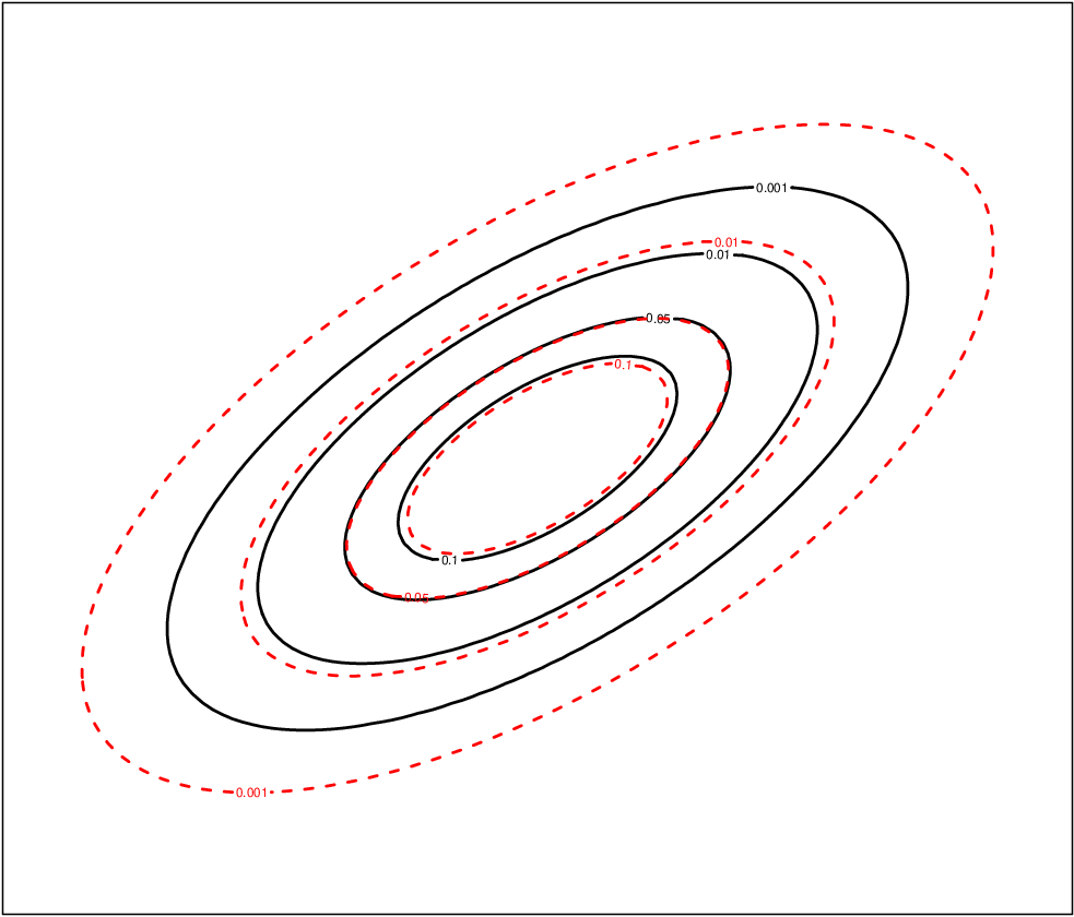
The density of our mixture of multivariate contaminated normal distributions is given by

Because our contaminated approach contains $2G$ components, i.e., $G$ top-level components, each of which contains two second-level components, the model in (1) shall be considered to contain $G$ clusters, rather than $G$ components, hereafter. Based on this consideration, model (5) can be seen as a special case of the multi-layer mixture of normal distributions of Li (2005) if each of the $G$ clusters at the top level is itself a mixture of two components, with equal means and proportional covariance matrices at the secondary layer.

Because there are $p\left(p+1\right)/2$ free parameters for each $\boldsymbol{\Sigma}_{g}$, it is usually necessary to introduce parsimony into the model in (5). Following Banfield and Raftery (1993) and Celeux and Govaert (1995), we consider the eigen-decomposition

where $\lambda_{g}=\left|\boldsymbol{\Sigma}_{g}\right|^{1/p}$, $\boldsymbol{\Delta}_{g}$ is the scaled ($\left|\boldsymbol{\Delta}_{g}\right|=1$) diagonal matrix of the eigenvalues of $\boldsymbol{\Sigma}_{g}$ sorted in decreasing order, and $\boldsymbol{\Gamma}_{g}$ is a $p\times p$ orthogonal matrix whose columns are the normalized eigenvectors of $\boldsymbol{\Sigma}_{g}$, ordered according to their eigenvalues. Each element in the right-hand side of (6) has a different geometric interpretation: $\lambda_{g}$ determines the volume of the $g$th cluster of the good data only, $\boldsymbol{\Delta}_{g}$ determines the shape of the cluster, and $\boldsymbol{\Gamma}_{g}$ determines the orientation of the cluster. Based on (4), the volume of the cluster is given by $\lambda_{g}\left[\alpha_{g}+\left(1-\alpha_{g}\right)\eta_{g}\right]$.

In the fashion of Celeux and Govaert (1995), we impose constraints on the three components of (6) resulting in a family of fourteen parsimonious mixtures of contaminated normal distributions models (Table 1). The last column of Table 1 specifies the scale invariant models of this family.

The idea of defining clustering in terms of the components of a mixture model goes back at least 60 years (cf. McNicholas, 2016, Section 2.1), and model-based clustering has become increasingly popular since mixture models were first used for clustering (Wolfe, 1965). Consider $n$ independent $p$-dimensional unlabeled observations $\left\{\boldsymbol{x}_{i}\right\}_{i=1}^{n}$ from model (5), and let $\left\{\boldsymbol{z}_{i}\right\}_{i=1}^{n}$ denote cluster memberships, where $\boldsymbol{z}_{i}=\left(z_{i1},\ldots,z_{iG}\right)^{\prime}$ and $z_{ig}=1$ if $\boldsymbol{x}_{i}$ belongs to cluster $g$ and $z_{ig}=0$ otherwise. Using the same notation as before, the model-based clustering likelihood is given by

and the predicted classifications are given by the maximum a posteriori probabilities (MAP). Note that

where

is the a posteriori expected value of $Z_{ig}$ given $\boldsymbol{x}_{i}$, i.e., the probability that $Z_{ig}=1$ given $\boldsymbol{x}_{i}$ and based on the parameter estimates $\widehat{\boldsymbol{\psi}}$.

To fit the models of our family, we use the expectation-conditional maximization (ECM) algorithm (Meng and Rubin, 1993). The ECM algorithm is a variant of the classical expectation-maximization (EM) algorithm (Dempster et al., 1977), which is a natural approach for maximum likelihood estimation when data are incomplete. In our case, there are two sources of missing data: one arises from the fact that we do not know the cluster labels $\left\{\boldsymbol{z}_{i}\right\}_{i=1}^{n}$ and the other arises from the fact that we do not know whether an observation in group $g$ is good or bad. To denote this second source of missing data, we use $\left\{\boldsymbol{v}_{i}\right\}_{i=1}^{n}$, where $\boldsymbol{v}_{i}=\left(v_{i1},\ldots,v_{iG}\right)^{\prime}$ so that $v_{ig}=1$ if observation $i$ in group $g$ is good and $v_{ig}=0$ if observation $i$ in group $g$ is bad. Therefore, the complete-data are given by $\mathcal{S}=\left\{\boldsymbol{x}_{i},\boldsymbol{z}_{i},\boldsymbol{v}_{i}\right\}_{i=1}^{n}$, and the complete-data log-likelihood can be written

where

with $\boldsymbol{\alpha}=\left(\alpha_{1},\ldots,\alpha_{G}\right)^{\prime}$ and $\boldsymbol{\theta}=\left\{\boldsymbol{\mu}_{g},\boldsymbol{\Sigma}_{g},\eta_{g}\right\}_{g=1}^{G}$. The ECM algorithm iterates between three steps, an E-step and two CM-steps, until convergence. The only difference from the EM algorithm is that each M-step is replaced by two simpler CM-steps. They arise from the partition $\boldsymbol{\psi}=\left\{\boldsymbol{\psi}_{1},\boldsymbol{\psi}_{2}\right\}$, where $\boldsymbol{\psi}_{1}=\left\{\pi_{g},\alpha_{g},\boldsymbol{\mu}_{g},\boldsymbol{\Sigma}_{g}\right\}_{g=1}^{G}$ and $\boldsymbol{\psi}_{2}=\left\{\eta_{g}\right\}_{g=1}^{G}$.

Here, we detail the ECM algorithm for the most general VVV model (5) under no constraint for $\alpha_{g}$, i.e., $\alpha_{g}\in\left(0,1\right)$, $g=1,\ldots,G$.

The ECM algorithm for the other models of our family changes only with respect to the way the terms of the eigen-decomposition of $\boldsymbol{\Sigma}_{g}$ are obtained in the first CM-step. In particular, these updates are analogous to those given by Celeux and Govaert (1995). The only difference is that, on the $\left(r+1\right)$th iteration of the algorithm, $\boldsymbol{W}_{g}^{\left(r+1\right)}$ is used instead of the classical scatter matrix

R source code implementing the ECM algorithm for all of the models of our family, in the form of an R package, is available from CRAN at https://cran.r-project.org/web/package=ContaminatedMixt (Punzo et al., 2015). As a basis to implement our code, we used the mixture package (Browne and McNicholas, 2015) for R (R Core Team, 2015), which gives a flexible implementation of the EM algorithm for the family of parsimonious mixtures of multivariate normal distributions introduced by Celeux and Govaert (1995), hereafter abbreviated as GPCM family. The mixture package differs from the Rmixmod package (Biernacki et al., 2008; Lebret et al., 2012) with respect to the algorithm used in the M-step to estimate parameters for the EVE and VVE models. In particular, the Rmixmod package adopts the classical FG-algorithm of Flury and Gautschi (1986), while the mixture package makes use of majorization-minimization (MM) algorithms (Hunter and Lange, 2000; Browne and McNicholas, 2014).

The choice of the starting values for EM-based algorithms constitutes an important issue (see, e.g., Biernacki et al., 2003, Karlis and Xekalaki, 2003, and Bagnato and Punzo, 2013). For the ECM algorithm described before, two natural strategies are:

1. 1.

   providing the initial quantities $\boldsymbol{z}_{i}^{\left(0\right)}$, $\boldsymbol{v}_{i}^{\left(0\right)}$, and $\eta_{g}^{\left(0\right)}$, $i=1,\ldots,n$ and $g=1,\ldots,G$, to the first CM-step of the first iteration; and

2. 2.

   selecting an initial value $\boldsymbol{\psi}^{\left(0\right)}$ for $\boldsymbol{\psi}$ in order to run the E-step of the first iteration.

By considering the first strategy, we suggest the following technique. Each ($G$-cluster) model of the GPCM family tends to the corresponding ($G$-cluster) model of our family when $\alpha_{g}\rightarrow 1^{-}$ and $\eta_{g}\rightarrow 1^{+}$, $g=1,\ldots,G$. Under these conditions, $v_{ig}\rightarrow 1^{-}$, $i=1,\ldots,n$ and $g=1,\ldots,G$. Then, the posterior probabilities from the EM algorithm for each model of the GPCM family — obtained with the gpcm() function of the mixture package — along with the constraints $v_{ig}^{\left(0\right)}=v^{\left(0\right)}$, with $v^{\left(0\right)}\rightarrow 1^{-}$, and $\eta_{g}=\eta^{\left(0\right)}$, with $\eta^{\left(0\right)}\rightarrow 1^{+}$, $i=1,\ldots,n$, and $g=1,\ldots,G$, can be used to run the first CM-step of the first iteration of our ECM algorithm. From an operational point of view, thanks to the monotonicity property of the ECM algorithm (see, e.g., McLachlan and Krishnan, 2007, p. 28), this also guarantees that the observed-data log-likelihood of a model from our family will be always greater than or equal to the observed-data log-likelihood of the corresponding model of the GPCM family (nested models); this is a fundamental consideration for the use of likelihood-based model selection criteria for choosing between models of our family and of the GPCM family (cf. Böhning and Ruangroj, 2002 and Punzo et al., 2016). In the analyses of Section 7, $v^{\left(0\right)}=0.999$ and $\eta^{\left(0\right)}=1.001$.

The Aitken acceleration (Aitken, 1926) is used to estimate the asymptotic maximum of the log-likelihood at each iteration of the ECM algorithm. Based on this estimate, we can decide whether or not the algorithm has reached convergence, i.e., whether or not the log-likelihood is sufficiently close to its estimated asymptotic value. The Aitken acceleration at iteration $r+1$ is given by

where $l^{\left(r\right)}$ is the observed-data log-likelihood value from iteration $r$. Then, the asymptotic estimate of the log-likelihood at iteration $r+2$ is given by

cf. Böhning et al. (1994). The ECM algorithm can be considered to have converged when $l_{\infty}^{\left(r+2\right)}-l^{\left(r+1\right)}<\epsilon$, with $\epsilon>0$, provided that this difference is positive (McNicholas et al., 2010). In our analyses, we use $\epsilon=0.0001$.

In the case of normal mixtures, it is well-known that the likelihood function: (1) presents spurious local maxima and (2) is unbounded. It tends to infinity when one of the cluster means coincides with a sample observation and the corresponding covariance matrix tends to be singular (Biernacki, 2004, cf.). The behaviour of the EM algorithm near a degenerate solution has been studied by Biernacki and Chrétien (2003), Ingrassia (2004), and Ingrassia and Rocci (2007); Ingrassia and Rocci (2011), who tackle the problem by constraining the value of the smallest eigenvalue of the cluster covariance matrices (see also Hathaway, 1986, for the univariate case). Recently, Browne et al. (2013) consider constraining the smallest eigenvalue, the largest eigenvalue, and both the smallest and largest eigenvalues for a subset of models of the GPCM family. However, all these approaches require an a priori choice of the constraints they are based on and no rule of thumb is given to assist this choice. Because further study of the best threshold values for these techniques is beyond the scope of this work, we avoid considering “preventive” approaches in the implementation of the ECM algorithm.

Based on (16), $\boldsymbol{\mu}_{g}^{\left(r+1\right)}$ is a weighted mean of the $\boldsymbol{x}_{i}$ values, with weights depending on

Consider the update for $v_{ig}^{\left(r\right)}$, given in (15), as a function of the squared Mahalanobis distance $\delta$, i.e.,

with $\delta\geq 0$. Due to the constraint $\eta_{g}>1$, from the last expression of (20) it is straightforward to realize that $h\left(\delta;\alpha_{g},\eta_{g}\right)$ is a decreasing function of $\delta$. Based on (20), (19) can be written

From the last expression of (21), $w\left(\delta;\alpha_{g},\eta_{g}\right)$ is an increasing function of $h\left(\delta;\alpha_{g},\eta_{g}\right)$; this also means that $w\left(\delta;\alpha_{g},\eta_{g}\right)$ is a decreasing function of $\delta$. Therefore, the weights in (19) reduce the impact of bad points in the estimation of the means $\boldsymbol{\mu}_{g}$, thereby providing robust estimates of these means. In addition, from (17), the larger $\delta$ values also have smaller effect on $\boldsymbol{\Sigma}_{g}$, $g=1,\ldots,G$, due to the weights in (19). For a discussion on down-weighting for the contaminated normal distribution, see also Little (1988).

For a model belonging to our family, the classification of an observation $\boldsymbol{x}_{i}$ means:

Step 1.

determine its cluster of membership;

Step 2.

establish whether it is a good or a bad observation in that cluster.

Let $\widehat{\boldsymbol{z}}_{i}$ and $\widehat{\boldsymbol{v}}_{i}$ denote, respectively, the expected values of $\boldsymbol{z}_{i}$ and $\boldsymbol{v}_{i}$ arising from the ECM algorithm, i.e., $\widehat{z}_{ig}$ is the value of $z_{ig}^{\left(r\right)}$ at convergence and $\widehat{v}_{ig}$ is the value of $v_{ig}^{\left(r\right)}$ at convergence. To evaluate the cluster membership of $\boldsymbol{x}_{i}$, we use the MAP classification, i.e., $\text{MAP}\left(\widehat{z}_{ig}\right)$. We then consider $\widehat{v}_{ih}$, where $h$ is selected such that $\text{MAP}\left(\widehat{z}_{ih}\right)=1$, and $\boldsymbol{x}_{i}$ is considered good if $\widehat{v}_{ih}>0.5$ and $\boldsymbol{x}_{i}$ is considered bad otherwise. The resulting information can be used to eliminate the bad points, if such an outcome is desired (Berkane and Bentler, 1988). The remaining data may then be treated as effectively being distributed according to a mixture of normal distributions, and the clustering results can be reported as usual. Finally, note that a a posteriori procedure (i.e., a procedure taking place once the model is fitted) to detect bad points with the mixture of multivariate $t$ distributions is illustrated by McLachlan and Peel (2000, p. 232). Such a procedure relies on a $\chi^{2}$-approximation, with $p$ degrees of freedom, of the squared Mahalanobis distances $\delta\left(\boldsymbol{x}_{i},\boldsymbol{\mu}_{g};\boldsymbol{\Sigma}_{g}\right)$, $i=1,\ldots,n$, after the MAP classification of each observation $\boldsymbol{x}_{i}$ to one of the $G$ groups, and it requires a subjective choice of a percentile of the $\chi^{2}$ distribution in order for the observation to be classified as good or bad; such a procedure will be applied, for comparison’s sake, in the analyses of Sections 6 and 7 by choosing the 95th percentile. On the contrary, the approach proposed herein is natural, in that it simultaneously identifies bad points and down-weights their impact on estimation of the mean (as well as on estimation of the covariance matrix; cf. Section 5.5), makes no additional distributional assumptions, and is not based on subjective choices.

When our models are used for detection of bad points in each group, $\left(1-\alpha_{g}\right)$ represents the proportion of bad points and $\eta_{g}$ denotes the degree of contamination. Then, for the former parameter, one could require that in the $g$th group, $g=1,\ldots,G$, the proportion of good data is at least equal to a pre-determined value $\alpha_{g}^{*}$. In this case, the optimize() function is also used for a numerical search of the maximum $\alpha_{g}^{\left(r+1\right)}$, over the interval $(\alpha_{g}^{*},1)$, of the function

In the analyses herein (Section 7), we use this approach to update $\alpha_{g}$ and, as emphasized in Section 2.1, we take $\alpha_{g}^{*}=0.5$, for $g=1,\ldots,G$. Note that it is also possible to fix $\alpha_{g}$ and/or $\eta_{g}$ a priori.

The models from our family, in addition to $\boldsymbol{\psi}$, are also characterized by the particular covariance structure and by the number of clusters $G$. Thus far, these quantities have been treated as a priori fixed; nevertheless, for practical purposes, model selection is usually required. One way (the usual way) to perform model selection is via computation of a convenient (likelihood-based) model selection criterion across all fourteen models and over a reasonable range of values for $G$, and then choosing the model associated with the best value of the adopted criterion (for the alternative use of likelihood-ratio tests to select either the parsimonious model or the number of components for a normal mixture, see Lo et al., 2001, Lo, 2005; Lo, 2008, and Punzo et al., 2016). Based on the simulation study performed by Li (2005) for the multi-layer mixture of normal distributions, in the data analyses of Section 7 we will adopt the Bayesian information criterion (Schwarz, 1978), i.e.,

where $m$ is the overall number of free parameters in the model. Note that, Bayes factors can be used to compare models that are not nested, and the BIC approximation thereto holds when models are not nested (cf. Raftery, 1995).

In this section, we investigate the behaviour of the proposed model (for simplicity, in its unconstrained version VVV) through a large-scale simulation study performed using R (R Core Team, 2015). We further provide a comparison with the unconstrained variants of the mixture models handling mild outliers and discussed in Section 1. A general feedback on advantages and drawbacks of each model is also given. We compare:

1. 1.

   mixture of normal distributions (abbreviated by NM = normal mixture). The gpcm() function of the mixture package (Browne and McNicholas, 2015) for R is used to fit the unconstrained normal mixture (corresponding to the VVV model based on the nomenclature of the mixture package). The gpcm() function implements the EM algorithm.

2. 2.

   mixture of $t$ distributions ($t$M = $t$ mixture; Andrews and McNicholas, 2012). The teigen() function of the teigen package (Andrews et al., 2015) for R is used to fit the unconstrained $t$ mixture (corresponding to the UUUU model with respect to the nomenclature of the teigen package). The teigen() function implements the ECM algorithm described, for example, in (Andrews et al., 2015). Degrees of freedom are estimated and they are allowed to vary across groups.

3. 3.

   mixture of contaminated normal distributions (CNM = contaminated normal mixture). The CNmixt() function of the ContaminatedMixt package (Punzo et al., 2015) for R is used to fit the unconstrained contaminated normal mixture (corresponding to the VVV model with respect to the nomenclature of the ContaminatedMixt package). The CNmixt() function implements the ECM algorithm described in Section 4.

4. 4.

   mixture of mixtures of a normal and a uniform distribution (NUM = normal-uniform mixture; Browne et al., 2012). A specific R code, implementing the generalized-EM (GEM) algorithm described in Browne et al. (2012), is used to fit the unconstrained normal-uniform mixture. No constraint is imposed on the component uniform distributions (corresponding to model IV with respect to the nomenclature of Browne et al., 2012).

5. 5.

   mixture of normal distributions plus a uniform component (NCM = noise component mixture; Banfield and Raftery, 1993). The Mclust() function of the mclust package (Fraley et al., 2012; Fraley et al., 2015) for R is used to fit the unconstrained noise component mixture (corresponding to the VVV model with respect to the nomenclature of the mclust package). The Mclust() function implements the EM algorithm.

To generate the data, we consider the following five data generation processes with $p=2$ dimensions and $G=2$ clusters:

1. a)

   NM;

2. b)

   $t$M with $\nu_{1}=4$ and $\nu_{2}=10$ degrees of freedom;

3. c)

   CNM with $\alpha_{1}=0.9$, $\alpha_{2}=0.8$, $\eta_{1}=20$, and $\eta_{2}=30$;

4. d)

   NM with 1% of points randomly substituted by high atypical points with coordinates $\left(0,x_{i2}^{*}\right)$, where $x_{i2}^{*}$ is generated from a uniform distribution over the interval $\left(10,15\right)$.

5. e)

   NM with 5% of points randomly substituted by noise points generated from a uniform distribution over the interval $\left(-10,10\right)$ on each dimension.

All of these data generation processes share the following common parameters

As concerns the mean in the first group, two alternatives are considered in order to reproduce two different degrees of overlap between clusters: $\boldsymbol{\mu}_{1}=\left(0,-3\right)^{\prime}$ in the “far” case, and $\boldsymbol{\mu}_{1}=\left(0,-1\right)^{\prime}$ in the “close” case. The five scenarios above cover different situations which may arise dealing with real-world data: no bad points for scenario a), heavy-tails cluster distributions for scenarios b) and c), and two different types of bad points for scenarios d) and e). Under each scenario, we simulate 1,000 samples considering the number of analyzed units $n$ (100, 200, and 500), as well as the degree of overlap (“far” and “close”), as experimental factors. This yields a total of 30,000 generated data sets. On each generated data set, the five competing models are directly run with $G=2$. As concerns the initialization strategy of the EM-based algorithms for the first four models (NM, $t$M, CNM, and NUM), the partition provided by the $k$-means method, as implemented by the kmeans() function, with default arguments, of the stats package for R, is considered. As concerns the NCM, an initial guess of the noise observations must be supplied via the noise component of the initialization argument in Mclust(). Nearest neighbor based clutter/noise detection proposed by Byers and Raftery (1998) is applied to identify an initial set of noise points. The latter is implemented in the NNclean() function in R’s prabclus package (Hennig and Hausdorf, 2015). Agglomerative hierarchical clustering based on ML criteria for normal mixtures proposed by Banfield and Raftery (1993) is then used for finding initial normal clusters in the non-noise data. This is implemented in the hc() function of R’s mclust package.

Before presenting the obtained results, we want to underline that the average elapsed time (in seconds over the 30,000 replications) to fit a single CNM is 0.692 seconds. This information is useful to have an idea of the computational burden required by our ECM algorithm. Computation is performed on a Windows 8.1 PC, with Intel i7 3.50GHz CPU, 16.0 GB RAM, using R 32 bit, and the elapsed time is computed via the proc.time() function of the base package.

For comparison’s sake, we report the bias (BIAS) and the standard deviation (STD) of the estimates for the mixture weight $\pi_{1}$, the univariate means $\mu_{11}$ and $\mu_{21}$ (elements of $\boldsymbol{\mu}_{1}$), and the univariate means $\mu_{12}$ and $\mu_{22}$ (elements of $\boldsymbol{\mu}_{2}$). Before to illustrate the obtained results, it is important to underline that under mixture models there are well known label switching issues (see, e.g., Celeux et al., 2000, Stephens, 2000, and Yao, 2012) when evaluating properties of the estimators of the parameters using simulation studies. There are no generally accepted labeling methods. In our simulation study, as in Bai et al. (2012) and Yao et al. (2014), we choose the labels by minimizing the distance to the true parameter values.

References

- Aggarwal (2013) Aggarwal, C. C., 2013. Outlier Analysis. Springer New York.
- Aitken (1926) Aitken, A., 1926. On Bernoulli’s numerical solution of algebraic equations. In: Proceedings of the Royal Society of Edinburgh. Vol. 46. pp. 289–305.
- Aitkin and Wilson (1980) Aitkin, M., Wilson, G. T., 1980. Mixture models, outliers, and the EM algorithm. Technometrics 22 (3), 325–331.
- Andrews and McNicholas (2012) Andrews, J. L., McNicholas, P. D., 2012. Model-based clustering, classification, and discriminant analysis with the multivariate -distribution: The EIGEN family. Statistics and Computing 22 (5), 1021–1029.
- Andrews et al. (2015)
Andrews, J. L., Wickins, J. R., Boers, N. M., McNicholas, P. D., 2015.
teigen: Model-Based Clustering and Classification with the
Multivariate Distribution. Version 2.1.0 (2015-11-20).
URL http://CRAN.R-project.org/package=teigen - Bagnato and Punzo (2013) Bagnato, L., Punzo, A., 2013. Finite mixtures of unimodal beta and gamma densities and the -bumps algorithm. Computational Statistics 28 (4), 1571–1597.
- Bai et al. (2012) Bai, X., Yao, W., Boyer, J. E., 2012. Robust fitting of mixture regression models. Computational Statistics & Data Analysis 56 (7), 2347–2359.
- Banfield and Raftery (1993) Banfield, J. D., Raftery, A. E., 1993. Model-based Gaussian and non-Gaussian clustering. Biometrics 49 (3), 803–821.
- Barnett and Lewis (1994) Barnett, V., Lewis, T., 1994. Outliers in Statistical Data. Wiley Series in Probability & Statistics. Wiley.
- Becker and Gather (1999) Becker, C., Gather, U., 1999. The masking breakdown point of multivariate outlier identification rules. Journal of the American Statistical Association 94 (447), 947–955.
- Berkane and Bentler (1988) Berkane, M., Bentler, P. M., 1988. Estimation of contamination parameters and identification of outliers in multivariate data. Sociological Methods & Research 17 (1), 55–64.
- Biernacki (2004) Biernacki, C., 2004. An asymptotic upper bound of the likelihood to prevent Gaussian mixtures from degenerating. Tech. rep., Université de Franche-Comté, Besançon.
- Biernacki et al. (2003) Biernacki, C., Celeux, G., Govaert, G., 2003. Choosing starting values for the EM algorithm for getting the highest likelihood in multivariate Gaussian mixture models. Computational Statistics & Data Analysis 41 (3-4), 561–575.
- Biernacki et al. (2008) Biernacki, C., Celeux, G., Govaert, G., Langrognet, F., Noulin, G., Vernaz, Y., 2008. - Statistical Documentation. Downloadable from http://www.mixmod.org/IMG/pdf/statdoc_2_1_1.pdf.
- Biernacki and Chrétien (2003) Biernacki, C., Chrétien, S., 2003. Degeneracy in the maximum likelihood estimation of univariate Gaussian mixtures with EM. Statistics & Probability Letters 61 (4), 373–382.
- Bock (2002) Bock, H. H., 2002. Clustering methods: From classical models to new approaches. Statistics in Transition 5 (5), 725–758.
- Böhning (2000) Böhning, D., 2000. Computer-assisted Analysis of Mixtures and Applications: Meta-analysis, Disease Mapping and Others. Vol. 81 of Monographs on Statistics and Applied Probability. Chapman & Hall/CRC, London.
- Böhning et al. (1994) Böhning, D., Dietz, E., Schaub, R., Schlattmann, P., Lindsay, B., 1994. The distribution of the likelihood ratio for mixtures of densities from the one-parameter exponential family. Annals of the Institute of Statistical Mathematics 46 (2), 373–388.
- Böhning and Ruangroj (2002) Böhning, D., Ruangroj, R., 2002. A note on the maximum deviation of the scale-contaminated normal to the best normal distribution. Metrika 55 (3), 177–182.
- Browne and McNicholas (2014) Browne, R. P., McNicholas, P. D., 2014. Estimating common principal components in high dimensions. Advances in Data Analysis and Classification 8 (2), 217–226.
- Browne and McNicholas (2015)
Browne, R. P., McNicholas, P. D., 2015. mixture: Mixture Models for
Clustering and Classification. Version 1.4 (2015-03-10).
URL http://CRAN.R-project.org/package=mixture - Browne et al. (2012) Browne, R. P., McNicholas, P. D., Sparling, M. D., 2012. Model-based learning using a mixture of mixtures of Gaussian and uniform distributions. IEEE Transactions on Pattern Analysis and Machine Intelligence 34 (4), 814–817.
- Browne et al. (2013) Browne, R. P., Subedi, S., McNicholas, P. D., 2013. Constrained optimization for a subset of the Gaussian parsimonious clustering models. arXiv.org e-print 1306.5824, available at: http://arxiv.org/abs/1306.5824.
- Byers and Raftery (1998) Byers, S., Raftery, A. E., 1998. Nearest-neighbor clutter removal for estimating features in spatial point processes. Journal of the American Statistical Association 93 (442), 577–584.
- Campbell (1984) Campbell, N. A., 1984. Mixture models and atypical values. Mathematical Geology 16 (5), 465–477.
- Campbell and Mahon (1974) Campbell, N. A., Mahon, R. J., 1974. A multivariate study of variation in two species of rock crab of genus Leptograpsus. Australian Journal of Zoology 22 (3), 417–425.
- Celeux and Govaert (1995) Celeux, G., Govaert, G., 1995. Gaussian parsimonious clustering models. Pattern Recognition 28 (5), 781–793.
- Celeux et al. (2000) Celeux, G., Hurn, M., Robert, C. P., 2000. Computational and inferential difficulties with mixture posterior distributions. Journal of the American Statistical Association 95 (451), 957–970.
- Coretto and Hennig (2011) Coretto, P., Hennig, C., 2011. Maximum likelihood estimation of heterogeneous mixtures of Gaussian and uniform distributions. Journal of Statistical Planning and Inference 141 (1), 462–473.
- Coretto and Hennig (2015) Coretto, P., Hennig, C., 2015. Robust improper maximum likelihood: tuning, computation, and a comparison with other methods for robust Gaussian clustering. arXiv.org e-print 1406.0808, available at: http://arxiv.org/abs/1406.0808.
- Crawford (1994) Crawford, S. L., 1994. An application of the laplace method to finite mixture distributions. Journal of the American Statistical Association 89 (425), 259–267.
- Cuesta-Albertos et al. (1997) Cuesta-Albertos, J. A., Gordaliza, A., Matrán, C., 1997. Trimmed -means: An attempt to robustify quantizers. The Annals of Statistics 25 (2), 553–576.
- Davies and Gather (1993) Davies, L., Gather, U., 1993. The identification of multiple outliers. Journal of the American Statistical Association 88 (423), 782–792.
- De Veaux and Krieger (1990) De Veaux, R. D., Krieger, A. M., 1990. Robust estimation of a normal mixture. Statistics & Probability Letters 10 (1), 1–7.
- Dempster et al. (1977) Dempster, A. P., Laird, N. M., Rubin, D. B., 1977. Maximum likelihood from incomplete data via the EM algorithm. Journal of the Royal Statistical Society: Series B (Statistical Methodology) 39 (1), 1–38.
- Di Zio et al. (2007) Di Zio, M., Guarnera, U., Rocci, R., 2007. A mixture of mixture models for a classification problem: The unity measure error. Computational Statistics & Data analysis 51 (5), 2573–2585.
- Flury and Gautschi (1986) Flury, B. N., Gautschi, W., 1986. An algorithm for simultaneous orthogonal transformation of several positive definite matrices to nearly diagonal form. SIAM Journal on Scientific and Statistical Computing 7 (1), 169–184.
- Forina et al. (1998) Forina, M., Leardi, R., Armanino, C., Lanteri, S., 1998. PARVUS: An extendible package for data exploration, classification and correlation. Tech. rep., Institute of Pharmaceutical and Food Analysis and Technologies, Genoa, Italy.
- Fraley and Raftery (1998) Fraley, C., Raftery, A. E., 1998. How many clusters? Which clustering method? Answers via model-based cluster analysis. Computer Journal 41 (8), 578–588.
- Fraley et al. (2012) Fraley, C., Raftery, A. E., Murphy, T. B., Scrucca, L., 2012. mclust version 4 for R: Normal mixture modeling for model-based clustering, classification, and density estimation. Technical report 597, Department of Statistics, University of Washington, Seattle, Washington, USA.
- Fraley et al. (2015)
Fraley, C., Raftery, A. E., Scrucca, L., Murphy, T. B., Fop, M., 2015.
mclust: Normal Mixture Modelling for Model-Based Clustering,
Classification, and Density Estimation. Version 5.1 (2015-10-27).
URL http://CRAN.R-project.org/package=mclust - Gallegos and Ritter (2005) Gallegos, M. T., Ritter, G., 2005. A robust method for cluster analysis. The Annals of Statistics 33 (1), 347–380.
- Gallegos and Ritter (2009) Gallegos, M. T., Ritter, G., 2009. Trimmed ML estimation of contaminated mixtures. Sankhyā: The Indian Journal of Statistics, Series A 71 (2), 164–220.
- García-Escudero and Gordaliza (1999) García-Escudero, L. A., Gordaliza, A., 1999. Robustness properties of means and trimmed means. Journal of the American Statistical Association 94 (447), 956–969.
- García-Escudero et al. (2003) García-Escudero, L. A., Gordaliza, A., Matrán, C., 2003. Trimming tools in exploratory data analysis. Journal of Computational and Graphical Statistics 12 (2), 434–449.
- García-Escudero et al. (2008) García-Escudero, L. A., Gordaliza, A., Matrán, C., Mayo-Iscar, A., 2008. A general trimming approach to robust cluster analysis. The Annals of Statistics 36 (3), 1324–1345.
- García-Escudero et al. (2010) García-Escudero, L. A., Gordaliza, A., Matrán, C., Mayo-Iscar, A., 2010. A review of robust clustering methods. Advances in Data Analysis and Classification 4 (2), 89–109.
- Gerogiannis et al. (2009) Gerogiannis, D., Nikou, C., Likas, A., 2009. The mixtures of Student’s t-distributions as a robust framework for rigid registration. Image and Vision Computing 27 (9), 1285–1294.
- Hartigan (1985) Hartigan, J. A., 1985. Statistical theory in clustering. Journal of classification 2 (1), 63–76.
- Hastie and Tibshirani (1996) Hastie, T., Tibshirani, R., 1996. Discriminant analysis by Gaussian mixtures. Journal of the Royal Statistical Society: Series B 58 (1), 155–176.
- Hathaway (1986) Hathaway, R. J., 1986. A constrained EM algorithm for univariate normal mixtures. Journal of Statistical Computation and Simulation 23 (3), 211–230.
- Hawkins (2013) Hawkins, D., 2013. Identification of Outliers. Monographs on Statistics and Applied Probability. Springer, The Netherlands.
- Hennig (2002) Hennig, C., 2002. Fixed point clusters for linear regression: computation and comparison. Journal of Classification 19 (2), 249–276.
- Hennig (2004) Hennig, C., 2004. Breakdown points for maximum likelihood estimators of location-scale mixtures. The Annals of Statistics 32 (4), 1313–1340.
- Hennig and Hausdorf (2015)
Hennig, C., Hausdorf, B., 2015. prabclus: Functions for Clustering of
Presence-Absence, Abundance and Multilocus Genetic Data. Version 2.2-6
(2015-01-14).
URL http://CRAN.R-project.org/package=prabclus - Holzmann et al. (2006) Holzmann, H., Munk, A., Gneiting, T., 2006. Identifiability of finite mixtures of elliptical distributions. Scandinavian Journal of Statistics 33 (4), 753–763.
- Hunter and Lange (2000) Hunter, D. R., Lange, K., 2000. Rejoinder to discussion of “optimization transfer using surrogate objective functions”. Journal of Computational and Graphical Statistics 9 (1), 52–59.
- Hurley (2004) Hurley, C., 2004. Clustering visualizations of multivariate data. Journal of Computational and Graphical Statistics 13 (4), 788–806.
- Ingrassia (2004) Ingrassia, S., 2004. A likelihood-based constrained algorithm for multivariate normal mixture models. Statistical Methods and Applications 13 (2), 151–166.
- Ingrassia and Rocci (2007) Ingrassia, S., Rocci, R., 2007. Constrained monotone em algorithms for finite mixture of multivariate Gaussians. Computational Statistics & Data Analysis 51 (11), 5339–5351.
- Ingrassia and Rocci (2011) Ingrassia, S., Rocci, R., 2011. Degeneracy of the EM algorithm for the mle of multivariate Gaussian mixtures and dynamic constraints. Computational Statistics & Data Analysis 55 (4), 1715–1725.
- Karlis and Xekalaki (2003) Karlis, D., Xekalaki, E., 2003. Choosing initial values for the EM algorithm for finite mixtures. Computational Statistics & Data Analysis 41 (3–4), 577–590.
- Lebret et al. (2012) Lebret, R., Iovleff, S., Langrognet, F., Biernacki, C., Celeux, G., Govaert, G., 2012. Rmixmod: The R Package of the Model-Based Unsupervised, Supervised and Semi-Supervised Classification Mixmod Library.
- Li (2005) Li, J., 2005. Clustering based on a multi-layer mixture model. Journal of Computational and Graphical Statistics 14 (3), 547–568.
- Little (1988) Little, R. J. A., 1988. Robust estimation of the mean and covariance matrix from data with missing values. Applied Statistics 37 (1), 23–38.
- Lo (2005) Lo, Y., 2005. Likelihood ratio tests of the number of components in a normal mixture with unequal variances. Statistics & Probability Letters 71 (3), 225–235.
- Lo (2008) Lo, Y., 2008. A likelihood ratio test of a homoscedastic normal mixture against a heteroscedastic normal mixture. Statistics and Computing 18 (3), 233–240.
- Lo et al. (2001) Lo, Y., Mendell, N. R., Rubin, D. B., 2001. Testing the number of components in a normal mixture. Biometrika 88 (3), 767–778.
- Markatou (2000) Markatou, M., 2000. Mixture models, robustness, and the weighted likelihood methodology. Biometrics 56 (2), 483–486.
- McLachlan and Krishnan (2007) McLachlan, G., Krishnan, T., 2007. The EM algorithm and extensions, 2nd Edition. Vol. 382 of Wiley Series in Probability and Statistics. John Wiley & Sons, New York.
- McLachlan and Basford (1988) McLachlan, G. J., Basford, K. E., 1988. Mixture Models: Inference and Applications to Clustering. Marcel Dekker, New York.
- McLachlan and Peel (1998) McLachlan, G. J., Peel, D., 1998. Robust cluster analysis via mixtures of multivariate -distributions. In: Amin, A., Dori, D., Pudil, P., Freeman, H. (Eds.), Advances in Pattern Recognition. Vol. 1451 of Lecture Notes in Computer Science. Springer, Berlin-Heidelberg, pp. 658–666.
- McLachlan and Peel (2000) McLachlan, G. J., Peel, D., 2000. Finite Mixture Models. John Wiley & Sons, New York.
- McNicholas (2010) McNicholas, P. D., 2010. Model-based classification using latent Gaussian mixture models. Journal of Statistical Planning and Inference 140 (5), 1175–1181.
- McNicholas (2016) McNicholas, P. D., 2016. Mixture Model-Based Classification. Chapman & Hall/CRC Press, Boca Raton.
- McNicholas et al. (2010) McNicholas, P. D., Murphy, T. B., McDaid, A. F., Frost, D., 2010. Serial and parallel implementations of model-based clustering via parsimonious Gaussian mixture models. Computational Statistics & Data Analysis 54 (3), 711–723.
- Meng and Rubin (1993) Meng, X.-L., Rubin, D. B., 1993. Maximum likelihood estimation via the ECM algorithm: A general framework. Biometrika 80 (2), 267–278.
- Peel and McLachlan (2000) Peel, D., McLachlan, G. J., 2000. Robust mixture modelling using the distribution. Statistics and Computing 10 (4), 339–348.
- Punzo et al. (2016) Punzo, A., Browne, R. P., McNicholas, P. D., 2016. Hypothesis testing for mixture model selection. Journal of Statistical Computation and Simulation. To appear, doi: 10.1080/00949655.2015.1131282.
- Punzo et al. (2015)
Punzo, A., Mazza, A., McNicholas, P. D., 2015. ContaminatedMixt:
Model-Based Clustering and Classification with the Multivariate Contaminated
Normal Distribution. Version 1.0 (2015-12-20).
URL http://CRAN.R-project.org/package=ContaminatedMixt - R Core Team (2015)
R Core Team, 2015. R: A Language and Environment for Statistical
Computing. R Foundation for Statistical Computing, Vienna, Austria.
URL http://www.R-project.org/ - Raftery (1995) Raftery, A. E., 1995. Bayesian model selection in social research. Sociological Methodology 25, 111–164.
- Ritter (2015) Ritter, G., 2015. Robust Cluster Analysis and Variable Selection. Vol. 137 of Chapman & Hall/CRC Monographs on Statistics & Applied Probability. CRC Press.
- Ruwet et al. (2012) Ruwet, C., García-Escudero, L. A., Gordaliza, A., Mayo-Iscar, A., 2012. The influence function of the tclust robust clustering procedure. Advances in Data Analysis and Classification 6 (2), 107–130.
- Ruwet et al. (2013) Ruwet, C., García-Escudero, L. A., Gordaliza, A., Mayo-Iscar, A., 2013. On the breakdown behavior of the tclust clustering procedure. Test 22 (3), 466–487.
- Schwarz (1978) Schwarz, G., 1978. Estimating the dimension of a model. The Annals of Statistics 6 (2), 461–464.
- Stephens (2000) Stephens, M., 2000. Dealing with label switching in mixture models. Journal of the Royal Statistical Society. Series B: Statistical Methodology 62 (4), 795–809.
- Teicher (1963) Teicher, H., 1963. Identifiability of finite mixtures. Annals of Mathematical Statistics 34 (4), 1265–1269.
- Tukey (1960) Tukey, J. W., 1960. A survey of sampling from contaminated distributions. In: Olkin, I. (Ed.), Contributions to Probability and Statistics: Essays in Honor of Harold Hotelling. Stanford Studies in Mathematics and Statistics. Stanford University Press, California, Ch. 39, pp. 448–485.
- Verdinelli and Wasserman (1991) Verdinelli, I., Wasserman, L., 1991. Bayesian analysis of outlier problems using the Gibbs sampler. Statistics and Computing 1 (2), 105–117.
- Wolfe (1965) Wolfe, J. H., 1965. A computer program for the maximum likelihood analysis of types. Technical Bulletin 65-15, U.S. Naval Personnel Research Activity.
- Yakowitz and Spragins (1968) Yakowitz, S. J., Spragins, J. D., 1968. On the identifiability of finite mixtures. The Annals of Mathematical Statistics 39 (1), 209–214.
- Yao (2012) Yao, W., 2012. Model based labeling for mixture models. Statistics and Computing 22 (2), 337–347.
- Yao et al. (2014) Yao, W., Wei, Y., Yu, C., 2014. Robust mixture regression using the -distribution. Computational Statistics & Data Analysis 71, 116–127.