Naturality in sutured monopole and instanton homologyThanks: JAB was partially supported by NSF Grant DMS-1104688. Thanks: SS was supported by NSF Postdoctoral Fellowship DMS-1204387.

John A. Baldwin Address: Department of Mathematics
Boston College Email address: john.baldwin@bc.edu and Steven Sivek Address: Department of Mathematics
Princeton University Email address: ssivek@math.princeton.edu

Abstract.

In [16], Kronheimer and Mrowka defined invariants of balanced sutured manifolds using monopole and instanton Floer homology. Their invariants assign isomorphism classes of modules to balanced sutured manifolds. In this paper, we introduce refinements of these invariants which assign much richer algebraic objects called projectively transitive systems of modules to balanced sutured manifolds and isomorphisms of such systems to diffeomorphisms of balanced sutured manifolds. Our work provides the foundation for extending these sutured Floer theories to other interesting functorial frameworks as well, and can be used to construct new invariants of contact structures and (perhaps) of knots and bordered 3-manifolds.

1. Introduction

In [16], Kronheimer and Mrowka defined invariants of balanced sutured manifolds using monopole and instanton Floer homology. The most basic versions of their monopole and instanton invariants assign isomorphism classes of finitely generated $\mathbb{Z}$ - and $\mathbb{C}$ -modules, denoted by $SHM(M,\gamma)$ and $SHI(M,\gamma)$ , respectively, to a balanced sutured manifold $(M,\gamma)$ . In this paper, we introduce refinements of Kronheimer and Mrowka’s invariants which assign much richer algebraic objects to balanced sutured manifolds. A similar program has recently been carried out in the realm of sutured (Heegaard) Floer homology ( $SFH$ ) by Juhász and Thurston [13]. These projects are motivated by a desire to fit these sutured Floer theories into interesting functorial frameworks (there are no interesting morphisms between isomorphism classes of modules). Some interesting source categories for such functors, with balanced sutured manifolds as objects, are:

(1)

DiffSut, whose morphisms are isotopy classes of diffeomorphisms of balanced sutured manifolds,
(2)

CobSut, whose morphisms are isomorphism classes of smooth cobordisms of balanced sutured manifolds, in the sense of [12],
(3)

ContSut, where the space of morphisms from $(M,\gamma)$ to $(M^{\prime},\gamma^{\prime})$ is empty unless the former is a sutured submanifold of the latter, in which case the morphism space consists of all isotopy classes of contact structures on $M^{\prime}\smallsetminus{\rm int}(M)$ for which $\partial M$ and $\partial M^{\prime}$ are convex with dividing sets $\gamma$ and $\gamma^{\prime}$ .

One natural target category for such functors is ${\mathcal{R}}{\mbox{-}}\textbf{{Mod}}{}$ , the category of $\mathcal{R}$ -modules for some commutative ring $\mathcal{R}$ . For example, the main result of [13] is that $SFH$ defines a functor from DiffSut to ${\mathbb{Z}/2}{\mbox{-}}\textbf{{Mod}}$ . Similarly, Juhász [12] and Honda, Kazez and Matić [11] have shown that $SFH$ extends to functors from CobSut and ContSut to ${\mathbb{Z}/2}{\mbox{-}}\textbf{{Mod}}$ .

The refinements of $SHM$ and $SHI$ constructed in this paper define functors from DiffSut (and certain full subcategories of DiffSut) to categories of projectively transitive systems which are closely related to ${\mathcal{R}}{\mbox{-}}\textbf{{Mod}}$ . We detour slightly in order to describe these categories.

1.1. $\mathcal{G}$ -Transitive Systems

Below, we generalize the notion of a transitive system of modules which was first introduced by Eilenberg and Steenrod in [6]. We will assume throughout that $\mathcal{R}$ is a commutative ring with $1$ .

Definition 1.1.

Fix a subgroup $\mathcal{G}\leq\mathcal{R}^{\times}$ and suppose $M_{\alpha},M_{\beta}$ are $\mathcal{R}$ -modules. Two homomorphisms $f,g:M_{\alpha}\to M_{\beta}$ are said to be $\mathcal{G}$ -equivalent if $f=u\cdot g$ for some $u\in\mathcal{G}$ .

We will write $f\doteq g$ to indicate that $f$ and $g$ are $\mathcal{R}^{\times}$ -equivalent. Observe that there is a well-defined notion of composition for $\mathcal{G}$ -equivalence classes.

Definition 1.2.

Fix a subgroup $\mathcal{G}\leq\mathcal{R}^{\times}$ . A $\mathcal{G}$ -transitive system of $\mathcal{R}$ -modules consists of a set $A$ together with:

(1)

a collection of $\mathcal{R}$ -modules $\{M_{\alpha}\}_{\alpha\in A}$ ,
(2)
a collection of $\mathcal{G}$ -equivalence classes $\{g^{\alpha}_{\beta}\}_{\alpha,\beta\in A}$ such that
1. (a)
  
  elements of $g^{\alpha}_{\beta}$ are isomorphisms from $M_{\alpha}$ to $M_{\beta}$ , for all $\alpha,\beta\in A$ ,
2. (b)
  
  $id_{M_{\alpha}}\in g^{\alpha}_{\alpha}$ , for all $\alpha\in A$ ,
3. (c)
  
  $g^{\beta}_{\gamma}\circ g^{\alpha}_{\beta}=g^{\alpha}_{\gamma}$ , for all $\alpha,\beta,\gamma\in A$ .

The module class of this system refers to the isomorphism class of the $\mathcal{R}$ -modules in $\{M_{\alpha}\}$ .

We will use the term projectively transitive system to refer to an $\mathcal{R}^{\times}$ -transitive system, while a transitive system, as defined in [6], is nothing other than a $\{1\}$ -transitive system.

Remark 1.3.

Just as the maps in a transitive system can be thought of as canonical isomorphisms, the $\mathcal{G}$ -equivalence classes in a $\mathcal{G}$ -transitive system can be thought of as specifying canonical isomorphisms that are well-defined up to multiplication by elements of $\mathcal{G}$ . Indeed, the point of introducing $\mathcal{G}$ -transitive systems is to make the latter notion precise.

Remark 1.4.

Note that a transitive system of $\mathcal{R}$ -modules $(A,\{M_{\alpha}\},\{g^{\alpha}_{\beta}\})$ canonically defines an actual $\mathcal{R}$ -module,

M=\coprod_{\alpha\in A}M_{\alpha}\big/{\sim},

where $m_{\alpha}\sim m_{\beta}$ iff $g^{\alpha}_{\beta}(m_{\alpha})=m_{\beta}$ , for $m_{\alpha}\in M_{\alpha}$ and $m_{\beta}\in M_{\beta}$ . So, the closer $\mathcal{G}$ is to $\{1\}$ , the closer a $\mathcal{G}$ -transitive system is to an actual $\mathcal{R}$ -module.

Definition 1.5.

A morphism of $\mathcal{G}$ -transitive systems from $(A,\{M_{\alpha}\},\{g^{\alpha}_{\beta}\})$ to $(B,\{N_{\gamma}\},\{h^{\gamma}_{\delta}\})$ is a collection of $\mathcal{G}$ -equivalence classes $\{f^{\alpha}_{\gamma}\}_{\alpha\in A,\,\gamma\in B}$ such that:

(1)

elements of $f^{\alpha}_{\gamma}$ are homomorphisms from $M_{\alpha}$ to $N_{\gamma}$ , for all $\alpha\in A$ and $\gamma\in B$ ,
(2)

$f^{\beta}_{\delta}\circ g^{\alpha}_{\beta}=h^{\gamma}_{\delta}\circ f^{\alpha}_{\gamma}$ , for all $\alpha,\beta\in A$ and $\gamma,\delta\in B$ .

With a notion of morphism in place, one can talk about the category of $\mathcal{G}$ -transitive systems of $\mathcal{R}$ -modules. In this paper, we will be concerned primarily with the categories ${\mathcal{R}}{\mbox{-}}\textbf{{Sys}}$ and ${\mathcal{R}}{\mbox{-}}\textbf{{PSys}}$ of transitive and projectively transitive systems of $\mathcal{R}$ -modules.

Remark 1.6.

Note that the assignment of modules to transitive systems above defines a canonical functor from ${\mathcal{R}}{\mbox{-}}\textbf{{Sys}}$ to ${\mathcal{R}}{\mbox{-}}\textbf{{Mod}}$ .

Remark 1.7.

For context, it is worth noting that what Juhász and Thurston really prove in [13] is that $SFH$ defines a functor from DiffSut to ${\mathbb{Z}/2}{\mbox{-}}\textbf{{Sys}}$ . Composing with the canonical functor from ${\mathbb{Z}/2}{\mbox{-}}\textbf{{Sys}}$ to ${\mathbb{Z}/2}{\mbox{-}}\textbf{{Mod}}$ then produces the functor from DiffSut to ${\mathbb{Z}/2}{\mbox{-}}\textbf{{Mod}}$ described in [13, Theorem 1.9].

As mentioned above, our refinements of $SHM$ and $SHI$ define functors from DiffSut to ${\mathcal{R}}{\mbox{-}}\textbf{{PSys}}$ for certain rings $\mathcal{R}$ . We describe these functors and rings in more detail below.

1.2. Our Refinements

Kronheimer and Mrowka’s invariants are defined in terms of closures of balanced sutured manifolds. A closure of $(M,\gamma)$ is a closed 3-manifold formed by gluing some auxiliary piece to $(M,\gamma)$ and then “closing up” by identifying the remaining boundary components, together with a distinguished surface in this closed manifold. Kronheimer and Mrowka assign modules to each such closure, defined in terms of the monopole and instanton Floer groups of the closed manifold relative to the distinguished surface, and they show that the modules assigned to different closures are isomorphic. So, the invariant objects they assign to $(M,\gamma)$ are the isomorphism classes, $SHM(M,\gamma)$ and $SHI(M,\gamma)$ , of these modules.

To extract invariant modules rather than mere isomorphism classes from Kronheimer and Mrowka’s constructions, one must show that the modules assigned to different closures are related by canonical isomorphisms, meaning that they fit into a transitive system. We do not quite go that far in this paper (see Subsection 1.4), but we prove something similar. With our (twisted) refinements of $SHM$ and $SHI$ , we show, for each theory, that the modules assigned to different closures are related by canonical isomorphisms that are well-defined up to multiplication by a unit, meaning that they fit into a projectively transitive system.

Our refinements of $SHM$ and $SHI$ start with refined notions of closure. For us, a closure of $(M,\gamma)$ is a tuple, commonly denoted by $\mathscr{D}$ , which records not only the manifold obtained by closing up $(M,\gamma)$ and the distinguished surface therein, but also the embedding of $M$ into this manifold and a tubular neighborhood of the distinguished surface. The genus of a closure refers to the genus of this surface. We describe these refinements below, beginning with those of $SHM$ .

Our primary focus in this paper is on a version of $SHM$ with twisted coefficients. This version and its refinement are based on a notion of marked closure, which also keeps track of a curve on the distinguished surface. This curve is used to define a twisted coefficient system over a ring $\mathcal{R}$ , where $\mathcal{R}$ belongs to a particular class of rings defined below.

Definition 1.8.

A Novikov-type ring is a commutative ring $\mathcal{R}$ with $1$ , equipped with a homomorphism ${\rm exp}:{\mathbb{R}}\rightarrow\mathcal{R}^{\times}$ such that

(1)

$\mathcal{R}$ does not contain any $\mathbb{Z}$ -torsion,
(2)

$t-t^{-1}$ is invertible, where $t^{\alpha}:={\rm exp}(\alpha)$ .

The prototypical example is the Novikov ring itself,

\bigg\{\sum_{\alpha}c_{\alpha}t^{\alpha}\,\bigg|\,\alpha\in\mathbb{R},\,c_{\alpha}\in\mathbb{Z},\,\#\{\beta<n|c_{\beta}\neq 0\}<\infty\bigg\},

with ${\rm exp}(\alpha)=t^{\alpha}$ and $(t-t^{-1})^{-1}=-t-t^{3}-t^{5}-\dots$ .

We will assume henceforth that $\mathcal{R}$ is some fixed Novikov-type ring.

Suppose $(M,\gamma)$ is a balanced sutured manifold. To every marked closure $\mathscr{D}$ of $(M,\gamma)$ , we assign an $\mathcal{R}$ -module $\underline{SHM}(\mathscr{D})$ in the isomorphism class $SHM(\mathscr{D})\otimes_{\mathbb{Z}}\mathcal{R}$ following the construction of $SHM$ with twisted (local) coefficients in [16, Definition 4.5]. For every pair $\mathscr{D},\mathscr{D}^{\prime}$ of marked closures, we construct an isomorphism

\underline{\Psi}_{\mathscr{D},\mathscr{D}^{\prime}}:\underline{SHM}(\mathscr{D})\to\underline{SHM}(\mathscr{D}^{\prime}),

well-defined up to multiplication by a unit in $\mathcal{R}$ , such that the transitivity

(1)

\underline{\Psi}_{\mathscr{D},\mathscr{D}^{\prime\prime}}\doteq\underline{\Psi}_{\mathscr{D}^{\prime},\mathscr{D}^{\prime\prime}}\circ\underline{\Psi}_{\mathscr{D},\mathscr{D}^{\prime}}

holds for every triple $\mathscr{D},\mathscr{D}^{\prime},\mathscr{D}^{\prime\prime}$ . Said differently, we construct canonical isomorphisms, well-defined up to multiplication by a unit in $\mathcal{R}$ , relating any pair of the modules in $\{\underline{SHM}(\mathscr{D})\}$ . These modules and isomorphisms therefore give rise to a projectively transitive system of $\mathcal{R}$ -modules, which we denote by $\textbf{{\lx@text@underline{SHM}}}(M,\gamma)$ and refer to as the twisted sutured monopole homology of $(M,\gamma)$ .

Given a diffeomorphism $f:(M,\gamma)\rightarrow(M^{\prime},\gamma^{\prime})$ , we define an isomorphism

(2)

\textbf{{\lx@text@underline{SHM}}}(f):\textbf{{\lx@text@underline{SHM}}}(M,\gamma)\rightarrow\textbf{{\lx@text@underline{SHM}}}(M^{\prime},\gamma^{\prime})

of projectively transitive systems of $\mathcal{R}$ -modules which depends only on the smooth isotopy class of $f$ . Furthermore, these isomorphisms satisfy

\textbf{{\lx@text@underline{SHM}}}(f^{\prime}\circ f)=\textbf{{\lx@text@underline{SHM}}}(f^{\prime})\circ\textbf{{\lx@text@underline{SHM}}}(f)

for diffeomorphisms

(M,\gamma)\xrightarrow{f}(M^{\prime},\gamma^{\prime})\xrightarrow{f^{\prime}}(M^{\prime\prime},\gamma^{\prime\prime}).

In particular, the mapping class group of $(M,\gamma)$ acts on $\textbf{{\lx@text@underline{SHM}}}(M,\gamma)$ . Thus, SHM defines a functor from DiffSut to $\mathcal{R}$ - $\textbf{{PSys}}.$ We restate this below in a weaker but more self-contained way which closely parallels [13, Theorem 1.9].

Theorem 1.9.

There exists a functor

\textbf{{\lx@text@underline{SHM}}}:\textup{{DiffSut}}\to{\mathcal{R}}{\mbox{-}}\textbf{{PSys}}

such that the module class of $\textbf{{\lx@text@underline{SHM}}}(M,\gamma)$ is equal to $SHM(M,\gamma)\otimes_{\mathbb{Z}}\mathcal{R}$ .

Our untwisted refinements are defined using ordinary closures. To every genus $g$ closure $\mathscr{D}$ of $(M,\gamma)$ , we assign a $\mathbb{Z}$ -module $SHM^{g}(\mathscr{D})$ in the isomorphism class $SHM(M,\gamma)$ following the construction in [16, Definition 4.3]. For each $g\geq 2$ and every pair $\mathscr{D},\mathscr{D}^{\prime}$ of genus $g$ closures, we construct an isomorphism

\Psi_{\mathscr{D},\mathscr{D}^{\prime}}^{g}:SHM^{g}(\mathscr{D})\to SHM^{g}(\mathscr{D}^{\prime}),

well-defined up to sign, such that

(3)

\Psi^{g}_{\mathscr{D},\mathscr{D}^{\prime\prime}}\doteq\Psi^{g}_{\mathscr{D}^{\prime},\mathscr{D}^{\prime\prime}}\circ\Psi^{g}_{\mathscr{D},\mathscr{D}^{\prime}}

for every triple $\mathscr{D},\mathscr{D}^{\prime},\mathscr{D}^{\prime\prime}$ . These modules and maps therefore give rise to a projectively transitive system of $\mathbb{Z}$ -modules, which we denote by $\textbf{{SHM}}^{g}(M,\gamma)$ and refer to as the untwisted sutured monopole homology of $(M,\gamma)$ in genus $g$ .

One can assign isomorphisms of systems to diffeomorphisms of balanced sutured manifolds just as in the twisted case, and so this invariant defines a functor from $\textup{{DiffSut}}^{g}$ to ${\mathbb{Z}}{\mbox{-}}\textbf{{PSys}}$ , where $\textup{{DiffSut}}^{g}$ is the full subcategory of DiffSut consisting of balanced sutured manifolds which admit genus $g$ closures.

Theorem 1.10.

For each $g\geq 2$ , there exists a functor

\textbf{{SHM}}^{g}:\textup{{DiffSut}}^{g}\to{\mathbb{Z}}{\mbox{-}}\textbf{{PSys}}

such that the module class of $\textbf{{SHM}}^{g}(M,\gamma)$ is equal to $SHM(M,\gamma)$ . The functor

\textbf{{SHM}}^{g}\otimes_{\mathbb{Z}}\mathcal{R}:\textup{{DiffSut}}^{g}\to{\mathcal{R}}{\mbox{-}}\textbf{{PSys}}

is naturally isomorphic to the restriction of SHM to $\textup{{DiffSut}}^{g}$ .

In characteristic two, this construction produces functors $\textbf{{SHM}}^{g}(-;\mathbb{Z}/2)$ from $\textup{{DiffSut}}^{g}$ to ${\mathbb{Z}/2}{\mbox{-}}\textbf{{Sys}}$ . Composition with the canonical functor from ${\mathbb{Z}/2}{\mbox{-}}\textbf{{Sys}}$ to ${\mathbb{Z}/2}{\mbox{-}}\textbf{{Mod}}$ then produces functors from $\textup{{DiffSut}}^{g}$ to ${\mathbb{Z}/2}{\mbox{-}}\textbf{{Mod}}$ which, in an abuse of notation, we will also denote by $\textbf{{SHM}}^{g}(-;\mathbb{Z}/2)$ . This is summarized in the corollaries below.

Corollary 1.11.

For each $g\geq 2$ , there exists a functor

\textbf{{SHM}}^{g}(-;\mathbb{Z}/2):\textup{{DiffSut}}^{g}\to{\mathbb{Z}/2}{\mbox{-}}\textbf{{Sys}}

such that the module class of $\textbf{{SHM}}^{g}(M,\gamma;\mathbb{Z}/2)$ is equal to $SHM(M,\gamma;\mathbb{Z}/2)$ .

Corollary 1.12.

For each $g\geq 2$ , there exists a functor

\textbf{{SHM}}^{g}(-;\mathbb{Z}/2):\textup{{DiffSut}}^{g}\to{\mathbb{Z}/2}{\mbox{-}}\textbf{{Mod}}

such that $\textbf{{SHM}}^{g}(M,\gamma;\mathbb{Z}/2)$ is isomorphic to $SHM(M,\gamma;\mathbb{Z}/2)$ .

At first glance, these untwisted refinements of $SHM$ may seem preferable in that they can be made to assign transitive systems and modules rather than just projectively transitive systems to balanced sutured manifolds. On the other hand, we do not know how to naturally relate the $\textbf{{SHM}}^{g}$ for different $g$ . This is not important in practice but explains our aesthetic preference for the twisted refinement SHM, which naturally incorporates (marked) closures of every genus.

In [16], Kronheimer and Mrowka use their sutured monopole invariant to define an invariant of knots called monopole knot homology ( $KHM$ ). Given a knot $K$ in a closed 3-manifold $Y$ , they define $KHM(Y,K)$ to be the isomorphism class

KHM(Y,K):=SHM(Y\smallsetminus\nu(K),m\cup-m),

where $\nu(K)$ is a solid torus neighborhood of $K$ and $m$ and $-m$ are oppositely oriented meridians on $\partial\nu(K)$ . We provide twisted and untwisted refinements of this invariant. Our refinements are invariants of based knots, where a based knot in $Y$ is a knot $K\subset Y$ together with a basepoint $p\in K$ . These refinements take the forms of the functors described below.

Theorem 1.13.

There exists a functor

\textbf{{\lx@text@underline{KHM}}}:\textup{{BKnot}}\to{\mathcal{R}}{\mbox{-}}\textbf{{PSys}}\\

such that the module class of $\textbf{{\lx@text@underline{KHM}}}(Y,K,p)$ is equal to $KHM(Y,K)\otimes_{\mathbb{Z}}\mathcal{R}$ .

Theorem 1.14.

For each $g\geq 2$ , there exists a functor

\textbf{{KHM}}^{g}:\textup{{BKnot}}\to{\mathbb{Z}}{\mbox{-}}\textbf{{PSys}}

such that the module class of $\textbf{{KHM}}^{g}(Y,K,p)$ is equal to $KHM(Y,K)$ .

Above, BKnot is the category whose objects are based knots in 3-manifolds, and where the morphism space from $(Y,K,p)$ to $(Y^{\prime},K^{\prime},p^{\prime})$ consists of isotopy classes of diffeomorphisms from $(Y,K,p)$ to $(Y,K^{\prime},p^{\prime})$ . One should compare Theorems 1.13 and 1.14 to [13, Theorem 1.8]. As before, one can define untwisted invariants in characteristic two which take the forms of functors from BKnot to ${\mathbb{Z}/2}{\mbox{-}}\textbf{{Sys}}$ and ${\mathbb{Z}/2}{\mbox{-}}\textbf{{Mod}}$ . One can also define analogous invariants of based links, though we do not do so here.

One can similarly define an invariant of based, closed $3$ -manifolds, which assigns to a pair $(Y,p)$ the isomorphism class of

SHM(Y(p)):=SHM(Y\smallsetminus\nu(p)),

where $\nu(p)$ is a tubular neighborhood of $p$ . There are twisted and untwisted refinements of this invariant which, among other things, account for the fact that $Y(p)$ technically depends on the neighborhood $\nu(p)$ rather than just on $p$ . These refinements take the form of the functors below.

Theorem 1.15.

There exists a functor

\textbf{{\lx@text@underline{HM}}}:\textup{{BMfld}}\to{\mathcal{R}}{\mbox{-}}\textbf{{PSys}}\\

such that the module class of $\textbf{{\lx@text@underline{HM}}}(Y,p)$ is equal to $SHM(Y(p))\otimes_{\mathbb{Z}}\mathcal{R}$ .

Theorem 1.16.

For each $g\geq 2$ , there exists a functor

\textbf{{HM}}^{g}:\textup{{BMfld}}\to{\mathbb{Z}}{\mbox{-}}\textbf{{PSys}}

such that the module class of $\textbf{{HM}}^{g}(Y,p)$ is equal to $SHM(Y(p))$ .

Here, BMfld is the category whose objects are based, closed 3-manifolds, and where the morphism space from $(Y,p)$ to $(Y^{\prime},p^{\prime})$ consists of isotopy classes of diffeomorphisms from $(Y,p)$ to $(Y,p^{\prime})$ . One should compare Theorems 1.15 and 1.16 to [13, Theorem 1.5]. As above, one can also define untwisted invariants in characteristic two which take the forms of functors from BMfld to ${\mathbb{Z}/2}{\mbox{-}}\textbf{{Sys}}$ and ${\mathbb{Z}/2}{\mbox{-}}\textbf{{Mod}}$ .

Our refinements of $SHI$ come in untwisted and twisted flavors as well, defined in terms of odd closures and marked odd closures. As the basic forms of these refinements are virtually identical to those of $SHM$ , we will leave a more detailed discussion to Section 9 and simply state the analogues of Theorems 1.9 and 1.10 below.

Theorem 1.17.

There exists a functor

\textbf{{\lx@text@underline{SHI}}}:\textup{{DiffSut}}\to{{\mathbb{C}}}{\mbox{-}}\textbf{{PSys}}

such that the module class of $\textbf{{\lx@text@underline{SHI}}}(M,\gamma)$ is equal to $SHI(M,\gamma)$ .

Theorem 1.18.

For each $g\geq 2$ , there exists a functor

\textbf{{SHI}}^{g}:\textup{{DiffSut}}^{g}\to{{\mathbb{C}}}{\mbox{-}}\textbf{{PSys}}

such that the module class of $\textbf{{SHI}}^{g}(M,\gamma)$ is equal to $SHI(M,\gamma)$ .

In Section 9, we also define twisted and untwisted refinements of Kronheimer and Mrowka’s instanton knot homology ( $KHI$ ). These take the forms of functors KHI and $\textbf{{KHI}}^{g}$ from BKnot to ${{\mathbb{C}}}{\mbox{-}}\textbf{{PSys}}$ . Finally, we define analogues HI and $\textbf{{HI}}^{g}$ of the functors in Theorems 1.15 and 1.16.

The key innovation in this paper is an alternative geometric interpretation of the isomorphisms used by Kronheimer and Mrowka to relate the modules assigned to different closures of the same genus. In [16], these maps are defined in terms of certain splicing cobordisms from the disjoint union of one closure and a mapping torus to the other closure. Here, they are defined in terms of 2-handle cobordisms, based on the observation that two closures of the same genus are naturally related by surgery.

Our alternative approach has two main advantages. First, it makes the transitivity of these isomorphisms, as expressed in (1) and (3), transparent for closures of the same genus, and thereby enables us to define the invariants $\textbf{{SHM}}^{g}$ and $\textbf{{SHI}}^{g}$ with ease. Second, and most importantly, it allows us to prove, in the twisted setting, that these isomorphisms commute with the isomorphisms used by Kronheimer and Mrowka to relate the modules assigned to closures whose genera differ by one. Indeed, the latter isomorphisms are defined in terms of splicing cobordisms similar to those mentioned above, and these splicing cobordisms commute with the 2-handle cobordisms we use to define the former isomorphisms. This commutativity is what ultimately enables us to prove the transitivity in (1) for arbitrary triples of closures, and thereby define the invariants SHM and SHI.

1.3. Some Applications

Below, we discuss some applications of these “naturality” results, mostly in the context of twisted sutured monopole homology. Nearly all of what is said below applies equally well in the untwisted and instanton contexts.

One application is to define stronger invariants of contact manifolds with convex boundary. In [1], we use naturality to define such an invariant, which assigns to a contact structure $\xi$ on $(M,\gamma)$ , for which $\partial M$ is convex with dividing curve $\gamma$ , an element of the projectively transitive system $\textbf{{\lx@text@underline{SHM}}}(M,\gamma)$ , which can be thought of as a collection $\{c(\mathscr{D},\xi)\in\underline{SHM}(\mathscr{D})\}$ of elements that are well-defined up to multiplication by a unit in $\mathcal{R}$ , such that

\underline{\Psi}_{\mathscr{D},\mathscr{D}^{\prime}}(c(\mathscr{D},\xi))=c(\mathscr{D}^{\prime},\xi),

up to multiplication by a unit in $\mathcal{R}$ , for all marked closures $\mathscr{D},\mathscr{D}^{\prime}$ of $(M,\gamma)$ .

Naturality makes this a much stronger invariant than it would otherwise be. For example, suppose $\xi$ and $\xi^{\prime}$ are contact structures on diffeomorphic manifolds $(M,\gamma)$ and $(M^{\prime},\gamma^{\prime})$ with marked closures $\mathscr{D}$ and $\mathscr{D}^{\prime}$ . To show that $\xi$ and $\xi^{\prime}$ are not contactomorphic, it suffices to show that the map from $\underline{SHM}(\mathscr{D})$ to $\underline{SHM}(\mathscr{D}^{\prime})$ induced by any diffeomorphism from $(M,\gamma)$ to $(M^{\prime},\gamma^{\prime})$ sends $c(\mathscr{D},\xi)$ to an element which is not in the orbit of $c(\mathscr{D}^{\prime},{\xi^{\prime}})$ under the action of the mapping class group of $(M^{\prime},\gamma^{\prime})$ . By contrast, without naturality, one must to show that there is no isomorphism from $\underline{SHM}(\mathscr{D})$ to $\underline{SHM}(\mathscr{D}^{\prime})$ sending $c(\mathscr{D},\xi)$ to $c(\mathscr{D}^{\prime},{\xi^{\prime}})$ . In [20], Ozsváth and Stipsicz apply what is essentially the same principle to distinguish Legendrian knots $\mathcal{K}$ and $\mathcal{K}^{\prime}$ in the same smooth knot type $K$ and with the same classical invariants using the Legendrian invariant $\widehat{\mathfrak{L}}$ defined in [19]. Specifically, they show that $\widehat{\mathfrak{L}}(\mathcal{K})$ and $\widehat{\mathfrak{L}}(\mathcal{K^{\prime}})$ are not in the same orbit under the action of the mapping class group of $(S^{3},K)$ on the knot Floer homology $\widehat{HFK}(S^{3},K)$ , even though the two invariants are related by an automorphism of $\widehat{HFK}(S^{3},K)$ .

As mentioned at the beginning, one of the primary motivations for proving the naturality results in this paper was to set the foundation for extending $SHM$ and $SHI$ to other functorial frameworks. We have made some partial progress in this direction. In [1], we define maps on SHM associated to contact handle attachments. To extend SHM to a functor from ContSut to ${\mathcal{R}}{\mbox{-}}\textbf{{PSys}}$ , the only remaining step is to show that if two compositions of handle attachments represent the same contact cobordism, then the corresponding compositions of maps agree. We will do this in future work. Once we do, we will be able to define a “minus” (or “from”) version of KHM by following a scheme of Etnyre, Vela-Vick and Zarev for recovering the “minus” version of knot Floer homology from $SFH$ using bypass attachment maps [7]. In the meantime, we use these handle attachment maps in [1] to prove a monopole Floer analogue of Honda’s bypass exact triangle in $SFH$ .

Once we extend SHM to a functor from ContSut to ${\mathcal{R}}{\mbox{-}}\textbf{{PSys}}$ , we will then be able to extend it to a functor from CobSut to ${\mathcal{R}}{\mbox{-}}\textbf{{PSys}}$ following Juhász’s strategy in [12]. While interesting in its own right, the latter functor will also provide a way of defining monopole Floer invariants for bordered 3-manifolds. In bordered Heegaard Floer homology, as defined by Lipshitz, Ozsváth and Thurston in [18], one assigns a differential graded algebra $\mathcal{A}(F)$ to a parametrized closed surface $F$ and a right $\mathcal{A}_{\infty}$ module $\widehat{CFA}(Y)$ over ${\mathcal{A}(F)}$ to a 3-manifold $Y$ with an identification of $\partial Y$ with $F$ . In [26, 25], Zarev shows that $H_{*}(\mathcal{A}(F))$ and $H_{*}(\widehat{CFA}(Y))$ are naturally isomorphic to direct sums of $SFH$ groups, and he gives an interpretation of the algebra and module multiplications (on homology) in terms of Juhász’s sutured cobordism maps on $SFH$ [12]. Extending SHM to a functor from CobSut to ${\mathcal{R}}{\mbox{-}}\textbf{{PSys}}$ will enable us to define analogous bordered invariants on the monopole side by mimicking Zarev’s construction. Of course, this will not be sufficient to define a full bordered theory, complete with a pairing theorem (for that, we would also need to define the higher multiplications), but it will represent significant progress towards such a construction.

1.4. Further Remarks

A natural question is whether one can give refinements of Kronheimer and Mrowka’s sutured monopole and instanton homology theories which take the form of transitive systems rather than projectively transitive systems. It appears difficult to do so (in the monopole case, for instance) for the following reason: there are several places in our paper where we consider $\mathcal{R}$ -modules of the form

\smash{\mskip 2.0mu\raise 15.93944pt\hbox to0.0pt{\begin{turn} {$\widehat{\phantom{\mathit{HM}}}$} \end{turn}\hss}\mskip-2.0mu\mathit{HM}}{\vphantom{\widehat{\mathit{HM}}}}{}_{\bullet}(Y|R;\Gamma_{\eta})

where $Y$ is a mapping torus with fiber $R$ and $\Gamma_{\eta}$ is a local system determined by a curve $\eta\subset R$ (see Subsection 3.1). The fact that we can identify

\smash{\mskip 2.0mu\raise 15.93944pt\hbox to0.0pt{\begin{turn} {$\widehat{\phantom{\mathit{HM}}}$} \end{turn}\hss}\mskip-2.0mu\mathit{HM}}{\vphantom{\widehat{\mathit{HM}}}}{}_{\bullet}(Y|R;\Gamma_{\eta})\cong\mathcal{R}

is used crucially both in the definition of the maps $\underline{\Psi}_{\mathscr{D},\mathscr{D}^{\prime}}$ and the proof that these maps are well-defined up to multiplication by a unit in $\mathcal{R}$ . To construct a transitive system, one needs a canonical such identification, and we do not know how to choose one at present. A naive strategy is to consider a Lefschetz fibration $X\to D^{2}$ with fiber $R$ and boundary $Y$ and identify $1\in\mathcal{R}$ with the relative invariant of $X$ . However, the use of twisted (local) coefficients makes this impossible: to define the relative invariant, one needs a 2-chain $\nu\subset X$ with $\partial\nu=\eta$ , and no such $\nu$ exists in general. We are hopeful that a slightly different approach, which involves enlarging the indexing set for our systems, will ultimately allow us to define transitive systems, but we do not elaborate further here. It is worth mentioning that practically all applications of naturality that we have in mind will work just as well with projectively transitive systems as with transitive systems.

Another natural question is whether one can define a projectively transitive system across closures of different genera in the untwisted case. In the instanton case, the answer is “yes” given the natural isomorphism between $\textbf{{\lx@text@underline{SHI}}}^{g}$ and $\textbf{{SHI}}^{g}$ described in Theorem 9.21. However, as one still needs twisted coefficients to relate the Floer groups associated to closures of different genera, this point is hardly worth emphasizing. The question is more interesting in the monopole case, and we do not know the answer. Theorem 1.10 implies that there is a natural isomorphism

\textbf{{SHM}}^{g}\otimes_{\mathbb{Z}}\mathcal{R}\cong(\textbf{{SHM}}^{g+1}\otimes_{\mathbb{Z}}\mathcal{R})|_{\textup{{DiffSut}}^{g}}.

Yet, it is not at all clear how to construct from this a natural isomorphism

\textbf{{SHM}}^{g}\cong(\textbf{{SHM}}^{g+1})|_{\textup{{DiffSut}}^{g}}

which could then be used to extend the untwisted theory to a projectively transitive system of $\mathbb{Z}$ -modules across all genera.

1.5. Organization

Most of this paper is devoted to constructing the maps $\underline{\Psi}_{\mathscr{D},\mathscr{D}^{\prime}}$ , proving their well-definedness up to multiplication by a unit in $\mathcal{R}$ , and showing that they satisfy the transitivity in (1).

In Section 2, we introduce our refined notions of closure and marked closure. In Section 3, we provide the necessary background on monopole Floer homology and define the untwisted and twisted sutured monopole homology modules associated to closures and marked closures, essentially rehashing [16, Definitions 4.3 and 4.5]. Section 4 develops the tools we will use to show that the maps $\underline{\Psi}_{\mathscr{D},\mathscr{D}^{\prime}}$ are independent of the choices in their constructions. In Section 5, we define these maps, first for marked closures of the same genus (Subsection 5.1); then, for marked closures whose genera differ by one (Subsection 5.2); and finally, for arbitrary marked closures (Subsection 5.3). In the same section, we prove that the maps $\underline{\Psi}_{\mathscr{D},\mathscr{D}^{\prime}}$ are well-defined and that they satisfy the transitivity in (1). In Section 6, we construct the isomorphisms $\textbf{{\lx@text@underline{SHM}}}(f)$ described in (2) and prove that SHM defines a functor from DiffSut to ${\mathcal{R}}{\mbox{-}}\textbf{{PSys}}$ . Section 7 deals with untwisted theory. There, we define the maps $\Psi^{g}_{\mathscr{D},\mathscr{D}^{\prime}}$ and the functors $\textbf{{SHM}}^{g}$ , and we describe the relationship between the twisted and untwisted monopole invariants. In Section 8, we define the monopole knot homology functors KHM, $\textbf{{KHM}}^{g}$ , HM, and $\textbf{{\lx@text@underline{HM}}}^{g}$ . In Section 9, we adapt the above results to the instanton context, defining the functors SHI and $\textbf{{SHI}}^{g}$ and describing the relationship between the two. There, we also define the instanton knot homology functors KHI, $\textbf{{KHI}}^{g}$ , HI, and $\textbf{{\lx@text@underline{HI}}}^{g}$ .

We end with two appendices. In Appendix A, we collect results about the diffeomorphism group of a surface times an interval relative to its boundary. A key topological operation used in this paper is that of cutting a 3-manifold open along a surface and regluing by a diffeomorphism. As explained in Section 4, one can realize this operation via Dehn surgery. The results of Appendix A provide a canonical (up to isotopy) identification of the cut-open-and-reglued manifold with the corresponding Dehn-surgered manifold, which then provides a canonical identification of their Floer homologies. The results of Appendix A, applied to the case of a torus times an interval, are also important in our refinement of monopole knot homology. In Appendix B, we prove a non-vanishing result for the (monopole Floer) relative invariants of Lefschetz fibrations over a disk, which we will use to relate the cobordism maps corresponding to the above Dehn surgeries to the splicing cobordisms used by Kronheimer and Mrowka in [16].

1.6. Acknowledgements

We thank Jon Bloom, Ryan Budney, András Juhász, Peter Kronheimer and Tom Mrowka for helpful conversations. We also thank the anonymous referee for many helpful suggestions.

2. Closures of Sutured Manifolds

In this section, we describe refinements of Kronheimer and Mrowka’s notion of closure for balanced sutured manifolds. We will work explicitly in the smooth category throughout. In particular, for us, balanced sutured manifolds come with smooth structures.

Definition 2.1.

A balanced sutured manifold $(M,\gamma)$ consists of a compact, oriented, smooth 3-manifold $M$ and a union $\gamma$ of disjoint, oriented, smooth curves in $\partial M$ called sutures. Let $R(\gamma)=\partial M\smallsetminus\gamma$ , oriented as a subsurface of $\partial M$ . We require that

(1)

neither $M$ nor $R(\gamma)$ has closed components,
(2)

$R(\gamma)=R_{+}(\gamma)\sqcup R_{-}(\gamma)$ with $\partial\overline{R_{+}(\gamma)}=-\partial\overline{R_{-}(\gamma)}=\gamma$ ,
(3)

$\chi(R_{+}(\gamma))=\chi(R_{-}(\gamma))$ .

Suppose $A(\gamma)$ is a closed tubular neighborhood of $\gamma$ in $\partial M$ . Let $F$ be a compact, connected, oriented surface with $g(F)>0$ and $\pi_{0}(\partial F)\cong\pi_{0}(\gamma)$ . Let

h:\partial F\times[-1,1]\rightarrow A(\gamma)

be an orientation-reversing homeomorphism sending $\partial F\times\{\pm 1\}$ to $\partial(R_{\pm}(\gamma)\smallsetminus A(\gamma)).$ Consider the manifold

M^{\prime}=M\cup_{h}F\times[-1,1]

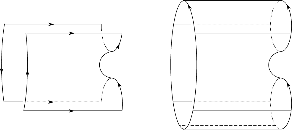
formed by gluing $F\times[-1,1]$ to $M$ according to $h$ and then rounding corners. Figure 1 shows a portion of $M^{\prime}$ . The fact that $(M,\gamma)$ is balanced ensures that $M^{\prime}$ has two homeomorphic boundary components, $\partial_{+}M^{\prime}$ and $\partial_{-}M^{\prime}$ . One can then glue $\partial_{+}M^{\prime}$ to $\partial_{-}M$ to form a closed manifold $Y$ containing a distinguished surface $R:=\partial_{+}M=\partial_{-}M$ . In [16], Kronheimer and Mrowka define a closure of $(M,\gamma)$ to be any pair $(Y,R)$ obtained in this way.

Refer to caption — Figure 1. Left, a portion of $M$ . The annulus $A(\gamma)$ is shown in gray and the regions marked $\pm$ are $R_{\pm}(\gamma)\smallsetminus A(\gamma)$ . Right, a portion of $M^{\prime}$ , showing part of $F\times[-1,1]$ glued to $M$ along $A(\gamma)$ after rounding corners.

Our notion of closure is somewhat more ambient. Rather than building $(Y,R)$ from $(M,\gamma)$ by the process described above, we start with a smooth manifold $Y$ into which $M$ and $R\times[-1,1]$ embed appropriately. Keeping track of these embeddings is what will allow us to define canonical isomorphisms (up to multiplication by a unit) between the monopole Floer invariants associated to different closures.

Definition 2.2.

A closure of $(M,\gamma)$ is a tuple $\mathscr{D}=(Y,R,r,m)$ consisting of:

(1)

a closed, oriented, smooth 3-manifold $Y$ ,
(2)

a closed, oriented, smooth surface $R$ with $g(R)\geq 2$ ,
(3)

a smooth, orientation-preserving embedding $r:R\times[-1,1]\hookrightarrow Y$ ,
(4)
a smooth, orientation-preserving embedding $m:M\hookrightarrow Y\smallsetminus{\rm int}({\rm Im}(r))$ such that
1. (a)
  
  $m$ extends to a diffeomorphism
  
  $M\cup_{h}F\times[-1,1]\rightarrow Y\smallsetminus{\rm int}({\rm Im}(r))$
  
  for some $A(\gamma)$ , $F$ , $h$ , as above, and some smooth structure on $M\cup_{h}F\times[-1,1]$ which restricts to the given smooth structure on $M$ ,
2. (b)
  
  $m$ restricts to an orientation-preserving embedding
  
  $R_{+}(\gamma)\smallsetminus A(\gamma)\hookrightarrow r(R\times\{-1\}).$

The genus $g(\mathscr{D})$ refers to the genus of $R$ .

Note that, for a closure $(Y,R,r,m)$ of $(M,\gamma)$ , the pair $(Y,r(R\times\{t\}))$ is a closure in the sense of Kronheimer and Mrowka, for any $t\in[-1,1]$ .

Definition 2.3.

A marked closure of $(M,\gamma)$ is a tuple $(Y,R,r,m,\eta)$ , where $(Y,R,r,m)$ is a closure of $(M,\gamma)$ , as defined above, and $\eta$ is an oriented, homologically essential, smoothly embedded curve in $R$ .

Marked closures are needed to define the twisted sutured monopole invariants that will be the focus of this paper.

3. Sutured Monopole Homology

In this section, we define the sutured monopole homology of a closure, closely following Kronheimer and Mrowka’s definition in [16, Definitions 4.3 and 4.4]. We begin with some background on monopole Floer homology for closed 3-manifolds. See [15, 16] for more details.

3.1. Monopole Floer Homology

Monopole Floer homology assigns to a closed, oriented, connected, smooth 3-manifold $Y$ a $\mathbb{Z}$ -module,

\smash{\mskip 2.0mu\raise 15.93944pt\hbox to0.0pt{\begin{turn} {$\widehat{\phantom{\mathit{HM}}}$} \end{turn}\hss}\mskip-2.0mu\mathit{HM}}{\vphantom{\widehat{\mathit{HM}}}}{}_{\bullet}(Y)=\bigoplus_{\mathfrak{s}\in\text{Spin}^{c}(Y)}\smash{\mskip 2.0mu\raise 15.93944pt\hbox to0.0pt{\begin{turn} {$\widehat{\phantom{\mathit{HM}}}$} \end{turn}\hss}\mskip-2.0mu\mathit{HM}}{\vphantom{\widehat{\mathit{HM}}}}{}_{\bullet}(Y,\mathfrak{s}).

More generally, $\smash{\mskip 2.0mu\raise 15.93944pt\hbox to0.0pt{\begin{turn} {$\widehat{\phantom{\mathit{HM}}}$} \end{turn}\hss}\mskip-2.0mu\mathit{HM}}{\vphantom{\widehat{\mathit{HM}}}}{}_{\bullet}$ is a functor from Cob to $\mathbb{Z}$ -Mod, where the objects of Cob are 3-manifolds as above and the morphisms are isomorphism classes of connected cobordisms with homology orientations (we will henceforth omit any mention of homology orientations, as we are only interested in cobordism maps up to sign). Here, a cobordism from $Y_{1}$ to $Y_{2}$ is a compact, oriented, smooth 4-manifold $W$ with boundary $\partial W=-\partial_{-}W\sqcup\partial_{+}W$ , together with orientation-preserving diffeomorphisms

\phi_{-}:\partial_{-}W\rightarrow Y_{1}{\rm\,\,\,\,\,and\,\,\,\,\,}\phi_{+}:\partial_{+}W\rightarrow Y_{2}.

Two cobordisms $(W,\phi_{\pm})$ and $(W^{\prime},\phi^{\prime}_{\pm})$ are isomorphic if there is an orientation-preserving diffeomorphism from $W$ to $W^{\prime}$ which intertwines the maps $\phi_{\pm}$ and $\phi^{\prime}_{\pm}$ . We will generally omit the diffeomorphisms $\phi_{\pm}$ from our notation and use

\smash{\mskip 2.0mu\raise 15.93944pt\hbox to0.0pt{\begin{turn} {$\widehat{\phantom{\mathit{HM}}}$} \end{turn}\hss}\mskip-2.0mu\mathit{HM}}{\vphantom{\widehat{\mathit{HM}}}}{}_{\bullet}(W):\smash{\mskip 2.0mu\raise 15.93944pt\hbox to0.0pt{\begin{turn} {$\widehat{\phantom{\mathit{HM}}}$} \end{turn}\hss}\mskip-2.0mu\mathit{HM}}{\vphantom{\widehat{\mathit{HM}}}}{}_{\bullet}(Y_{1})\to\smash{\mskip 2.0mu\raise 15.93944pt\hbox to0.0pt{\begin{turn} {$\widehat{\phantom{\mathit{HM}}}$} \end{turn}\hss}\mskip-2.0mu\mathit{HM}}{\vphantom{\widehat{\mathit{HM}}}}{}_{\bullet}(Y_{2})

to denote the map induced by $W$ . As this notation indicates, we will also blur the distinction between a cobordism and its isomorphism class.

Given cobordisms $W_{1}$ from $Y_{1}$ to $Y_{2}$ and $W_{2}$ from $Y_{2}$ to $Y_{3}$ , the composite $W_{3}=W_{2}\circ W_{1}$ from $Y_{1}$ to $Y_{3}$ is formed as the quotient of $W_{1}\sqcup W_{2}$ by the map

(\phi_{2})^{-1}_{-}\circ(\phi_{1})_{+}:\partial_{+}W_{1}\rightarrow\partial_{-}W_{2},

and is endowed with the natural boundary identifications $(\phi_{3})_{-}=(\phi_{1})_{-}$ and $(\phi_{3})_{+}=(\phi_{2})_{+}$ . The statement that $\smash{\mskip 2.0mu\raise 15.93944pt\hbox to0.0pt{\begin{turn} {$\widehat{\phantom{\mathit{HM}}}$} \end{turn}\hss}\mskip-2.0mu\mathit{HM}}{\vphantom{\widehat{\mathit{HM}}}}{}_{\bullet}$ is a functor implies that

(4)

\smash{\mskip 2.0mu\raise 15.93944pt\hbox to0.0pt{\begin{turn} {$\widehat{\phantom{\mathit{HM}}}$} \end{turn}\hss}\mskip-2.0mu\mathit{HM}}{\vphantom{\widehat{\mathit{HM}}}}{}_{\bullet}(W_{3})=\smash{\mskip 2.0mu\raise 15.93944pt\hbox to0.0pt{\begin{turn} {$\widehat{\phantom{\mathit{HM}}}$} \end{turn}\hss}\mskip-2.0mu\mathit{HM}}{\vphantom{\widehat{\mathit{HM}}}}{}_{\bullet}(W_{2})\circ\smash{\mskip 2.0mu\raise 15.93944pt\hbox to0.0pt{\begin{turn} {$\widehat{\phantom{\mathit{HM}}}$} \end{turn}\hss}\mskip-2.0mu\mathit{HM}}{\vphantom{\widehat{\mathit{HM}}}}{}_{\bullet}(W_{1}).

Given a smooth 1-cycle $\eta\subset Y$ , Kronheimer and Mrowka define a version of monopole Floer homology with twisted (local) coefficients which takes the form of an $\mathcal{R}$ -module,

\smash{\mskip 2.0mu\raise 15.93944pt\hbox to0.0pt{\begin{turn} {$\widehat{\phantom{\mathit{HM}}}$} \end{turn}\hss}\mskip-2.0mu\mathit{HM}}{\vphantom{\widehat{\mathit{HM}}}}{}_{\bullet}(Y;\Gamma_{\eta})=\bigoplus_{\mathfrak{s}\in\text{Spin}^{c}(Y)}\smash{\mskip 2.0mu\raise 15.93944pt\hbox to0.0pt{\begin{turn} {$\widehat{\phantom{\mathit{HM}}}$} \end{turn}\hss}\mskip-2.0mu\mathit{HM}}{\vphantom{\widehat{\mathit{HM}}}}{}_{\bullet}(Y,\mathfrak{s};\Gamma_{\eta}).

Suppose $\eta_{1}\subset Y_{1}$ and $\eta_{2}\subset Y_{2}$ are smooth 1-cycles. A cobordism from $(Y_{1},\eta_{1})$ to $(Y_{2},\eta_{2})$ is a cobordism $W$ as above together with a smooth relative 2-cycle $\nu\subset W$ such that $\partial\nu=\eta_{2}-\eta_{1}$ under the identifications $\phi_{\pm}$ . Such a cobordism $(W,\nu)$ induces a map

\smash{\mskip 2.0mu\raise 15.93944pt\hbox to0.0pt{\begin{turn} {$\widehat{\phantom{\mathit{HM}}}$} \end{turn}\hss}\mskip-2.0mu\mathit{HM}}{\vphantom{\widehat{\mathit{HM}}}}{}_{\bullet}(W;\Gamma_{\nu}):\smash{\mskip 2.0mu\raise 15.93944pt\hbox to0.0pt{\begin{turn} {$\widehat{\phantom{\mathit{HM}}}$} \end{turn}\hss}\mskip-2.0mu\mathit{HM}}{\vphantom{\widehat{\mathit{HM}}}}{}_{\bullet}(Y_{1};\Gamma_{\eta_{1}})\to\smash{\mskip 2.0mu\raise 15.93944pt\hbox to0.0pt{\begin{turn} {$\widehat{\phantom{\mathit{HM}}}$} \end{turn}\hss}\mskip-2.0mu\mathit{HM}}{\vphantom{\widehat{\mathit{HM}}}}{}_{\bullet}(Y_{2};\Gamma_{\eta_{2}})

which depends only on the homology class $[\nu]\subset H_{2}(W,\partial W;{\mathbb{R}})$ and the isomorphism class of $(W,\nu)$ , where $(W,\nu)$ and $(W^{\prime},\nu^{\prime})$ are isomorphic if there is a diffeomorphism from one pair to the other which intertwines the maps $\phi_{\pm}$ and $\phi_{\pm}^{\prime}$ . Composition of cobordisms is defined in the obvious way and the analogue of (4) holds in this setting as well.

The functoriality of $\smash{\mskip 2.0mu\raise 15.93944pt\hbox to0.0pt{\begin{turn} {$\widehat{\phantom{\mathit{HM}}}$} \end{turn}\hss}\mskip-2.0mu\mathit{HM}}{\vphantom{\widehat{\mathit{HM}}}}{}_{\bullet}$ can be used to assign isomorphisms on Floer homology to diffeomorphisms between 3-manifolds as follows. Suppose $\psi$ is an orientation-preserving diffeomorphism from $Y$ to $Y^{\prime}$ which sends a smooth 1-cycle $\eta\subset Y$ to $\eta^{\prime}\subset Y^{\prime}$ . Consider the cobordism $(W,\nu)=(Y\times[0,1],\eta\times[0,1])$ from $(Y,\eta)$ to $(Y^{\prime},\eta^{\prime})$ with boundary identifications

\phi_{-}=id:Y\times\{0\}\rightarrow Y\,\,\,\,\,{\rm and}\,\,\,\,\,\phi_{+}=\psi:Y\times\{1\}\rightarrow Y^{\prime}.

Then, the induced maps

	$\displaystyle\smash{\mskip 2.0mu\raise 15.93944pt\hbox to0.0pt{\begin{turn} {$\widehat{\phantom{\mathit{HM}}}$} \end{turn}\hss}\mskip-2.0mu\mathit{HM}}{\vphantom{\widehat{\mathit{HM}}}}{}_{\bullet}(\psi)$	$\displaystyle:=\smash{\mskip 2.0mu\raise 15.93944pt\hbox to0.0pt{\begin{turn} {$\widehat{\phantom{\mathit{HM}}}$} \end{turn}\hss}\mskip-2.0mu\mathit{HM}}{\vphantom{\widehat{\mathit{HM}}}}{}_{\bullet}(W):\smash{\mskip 2.0mu\raise 15.93944pt\hbox to0.0pt{\begin{turn} {$\widehat{\phantom{\mathit{HM}}}$} \end{turn}\hss}\mskip-2.0mu\mathit{HM}}{\vphantom{\widehat{\mathit{HM}}}}{}_{\bullet}(Y)\to\smash{\mskip 2.0mu\raise 15.93944pt\hbox to0.0pt{\begin{turn} {$\widehat{\phantom{\mathit{HM}}}$} \end{turn}\hss}\mskip-2.0mu\mathit{HM}}{\vphantom{\widehat{\mathit{HM}}}}{}_{\bullet}(Y^{\prime})$
	$\displaystyle\smash{\mskip 2.0mu\raise 15.93944pt\hbox to0.0pt{\begin{turn} {$\widehat{\phantom{\mathit{HM}}}$} \end{turn}\hss}\mskip-2.0mu\mathit{HM}}{\vphantom{\widehat{\mathit{HM}}}}{}_{\bullet}(\psi)$	$\displaystyle:=\smash{\mskip 2.0mu\raise 15.93944pt\hbox to0.0pt{\begin{turn} {$\widehat{\phantom{\mathit{HM}}}$} \end{turn}\hss}\mskip-2.0mu\mathit{HM}}{\vphantom{\widehat{\mathit{HM}}}}{}_{\bullet}(W;\Gamma_{\nu}):\smash{\mskip 2.0mu\raise 15.93944pt\hbox to0.0pt{\begin{turn} {$\widehat{\phantom{\mathit{HM}}}$} \end{turn}\hss}\mskip-2.0mu\mathit{HM}}{\vphantom{\widehat{\mathit{HM}}}}{}_{\bullet}(Y;\Gamma_{\eta})\to\smash{\mskip 2.0mu\raise 15.93944pt\hbox to0.0pt{\begin{turn} {$\widehat{\phantom{\mathit{HM}}}$} \end{turn}\hss}\mskip-2.0mu\mathit{HM}}{\vphantom{\widehat{\mathit{HM}}}}{}_{\bullet}(Y^{\prime};\Gamma_{\eta^{\prime}})$

are isomorphisms which depend only on the smooth isotopy class of $\psi$ (rel $\eta$ in the twisted case). Moreover, for diffeomorphisms $\psi_{1}$ from $(Y_{1},\eta_{1})$ to $(Y_{2},\eta_{2})$ and $\psi_{2}$ from $(Y_{2},\eta_{2})$ to $(Y_{3},\eta_{3})$ , we have that

\smash{\mskip 2.0mu\raise 15.93944pt\hbox to0.0pt{\begin{turn} {$\widehat{\phantom{\mathit{HM}}}$} \end{turn}\hss}\mskip-2.0mu\mathit{HM}}{\vphantom{\widehat{\mathit{HM}}}}{}_{\bullet}(\psi_{2}\circ\psi_{1})=\smash{\mskip 2.0mu\raise 15.93944pt\hbox to0.0pt{\begin{turn} {$\widehat{\phantom{\mathit{HM}}}$} \end{turn}\hss}\mskip-2.0mu\mathit{HM}}{\vphantom{\widehat{\mathit{HM}}}}{}_{\bullet}(\psi_{2})\circ\smash{\mskip 2.0mu\raise 15.93944pt\hbox to0.0pt{\begin{turn} {$\widehat{\phantom{\mathit{HM}}}$} \end{turn}\hss}\mskip-2.0mu\mathit{HM}}{\vphantom{\widehat{\mathit{HM}}}}{}_{\bullet}(\psi_{1}).

As a special case, these maps define actions of the mapping class groups of $Y$ and $(Y,\eta)$ on $\smash{\mskip 2.0mu\raise 15.93944pt\hbox to0.0pt{\begin{turn} {$\widehat{\phantom{\mathit{HM}}}$} \end{turn}\hss}\mskip-2.0mu\mathit{HM}}{\vphantom{\widehat{\mathit{HM}}}}{}_{\bullet}(Y)$ and $\smash{\mskip 2.0mu\raise 15.93944pt\hbox to0.0pt{\begin{turn} {$\widehat{\phantom{\mathit{HM}}}$} \end{turn}\hss}\mskip-2.0mu\mathit{HM}}{\vphantom{\widehat{\mathit{HM}}}}{}_{\bullet}(Y;\Gamma_{\eta})$ .

When defining monopole Floer invariants of sutured manifolds, we will be particularly interested in certain summands of $\smash{\mskip 2.0mu\raise 15.93944pt\hbox to0.0pt{\begin{turn} {$\widehat{\phantom{\mathit{HM}}}$} \end{turn}\hss}\mskip-2.0mu\mathit{HM}}{\vphantom{\widehat{\mathit{HM}}}}{}_{\bullet}$ . In general, the summands $\smash{\mskip 2.0mu\raise 15.93944pt\hbox to0.0pt{\begin{turn} {$\widehat{\phantom{\mathit{HM}}}$} \end{turn}\hss}\mskip-2.0mu\mathit{HM}}{\vphantom{\widehat{\mathit{HM}}}}{}_{\bullet}(Y,\mathfrak{s})\subset\smash{\mskip 2.0mu\raise 15.93944pt\hbox to0.0pt{\begin{turn} {$\widehat{\phantom{\mathit{HM}}}$} \end{turn}\hss}\mskip-2.0mu\mathit{HM}}{\vphantom{\widehat{\mathit{HM}}}}{}_{\bullet}(Y)$ are constrained by an adjunction inequality, which states that if $R\subset Y$ is a connected, oriented, smoothly embedded surface with $g(R)>0$ and $\smash{\mskip 2.0mu\raise 15.93944pt\hbox to0.0pt{\begin{turn} {$\widehat{\phantom{\mathit{HM}}}$} \end{turn}\hss}\mskip-2.0mu\mathit{HM}}{\vphantom{\widehat{\mathit{HM}}}}{}_{\bullet}(Y,\mathfrak{s})$ is nonzero, then

|\langle c_{1}(\mathfrak{s}),[R]\rangle|\leq 2g(R)-2.

For $R\subset Y$ as above, Kronheimer and Mrowka define the submodule $\smash{\mskip 2.0mu\raise 15.93944pt\hbox to0.0pt{\begin{turn} {$\widehat{\phantom{\mathit{HM}}}$} \end{turn}\hss}\mskip-2.0mu\mathit{HM}}{\vphantom{\widehat{\mathit{HM}}}}{}_{\bullet}(Y|R)\subset\smash{\mskip 2.0mu\raise 15.93944pt\hbox to0.0pt{\begin{turn} {$\widehat{\phantom{\mathit{HM}}}$} \end{turn}\hss}\mskip-2.0mu\mathit{HM}}{\vphantom{\widehat{\mathit{HM}}}}{}_{\bullet}(Y)$ to be the direct sum over “top” $\text{Spin}^{c}$ structures,

\smash{\mskip 2.0mu\raise 15.93944pt\hbox to0.0pt{\begin{turn} {$\widehat{\phantom{\mathit{HM}}}$} \end{turn}\hss}\mskip-2.0mu\mathit{HM}}{\vphantom{\widehat{\mathit{HM}}}}{}_{\bullet}(Y|R):=\bigoplus_{\langle c_{1}(\mathfrak{s}),[R]\rangle=2g(R)-2}\smash{\mskip 2.0mu\raise 15.93944pt\hbox to0.0pt{\begin{turn} {$\widehat{\phantom{\mathit{HM}}}$} \end{turn}\hss}\mskip-2.0mu\mathit{HM}}{\vphantom{\widehat{\mathit{HM}}}}{}_{\bullet}(Y,\mathfrak{s}).

The submodule $\smash{\mskip 2.0mu\raise 15.93944pt\hbox to0.0pt{\begin{turn} {$\widehat{\phantom{\mathit{HM}}}$} \end{turn}\hss}\mskip-2.0mu\mathit{HM}}{\vphantom{\widehat{\mathit{HM}}}}{}_{\bullet}(Y|R;\Gamma_{\eta})\subset\smash{\mskip 2.0mu\raise 15.93944pt\hbox to0.0pt{\begin{turn} {$\widehat{\phantom{\mathit{HM}}}$} \end{turn}\hss}\mskip-2.0mu\mathit{HM}}{\vphantom{\widehat{\mathit{HM}}}}{}_{\bullet}(Y;\Gamma_{\eta})$ is defined analogously.

Notation 3.1.

Given a 3-manifold $Y$ , a surface $R$ , a curve $\eta\subset R$ and an embedding $r:R\times[-1,1]\hookrightarrow Y$ , we will use the shorthand

	$\displaystyle\smash{\mskip 2.0mu\raise 15.93944pt\hbox to0.0pt{\begin{turn} {$\widehat{\phantom{\mathit{HM}}}$} \end{turn}\hss}\mskip-2.0mu\mathit{HM}}{\vphantom{\widehat{\mathit{HM}}}}{}_{\bullet}(Y\|R)\,\,\,\,$	$\displaystyle{\rm for}\,\,\,\,\smash{\mskip 2.0mu\raise 15.93944pt\hbox to0.0pt{\begin{turn} {$\widehat{\phantom{\mathit{HM}}}$} \end{turn}\hss}\mskip-2.0mu\mathit{HM}}{\vphantom{\widehat{\mathit{HM}}}}{}_{\bullet}(Y\|r(R\times\{0\}))$
	$\displaystyle\smash{\mskip 2.0mu\raise 15.93944pt\hbox to0.0pt{\begin{turn} {$\widehat{\phantom{\mathit{HM}}}$} \end{turn}\hss}\mskip-2.0mu\mathit{HM}}{\vphantom{\widehat{\mathit{HM}}}}{}_{\bullet}(Y\|R;\Gamma_{\eta})\,\,\,\,$	$\displaystyle{\rm for}\,\,\,\,\smash{\mskip 2.0mu\raise 15.93944pt\hbox to0.0pt{\begin{turn} {$\widehat{\phantom{\mathit{HM}}}$} \end{turn}\hss}\mskip-2.0mu\mathit{HM}}{\vphantom{\widehat{\mathit{HM}}}}{}_{\bullet}(Y\|r(R\times\{0\});\Gamma_{r(\eta\times\{0\})}).$

Example 3.2.

Suppose $R$ is a smooth surface with $g(R)\geq 2$ , $\phi$ is an orientation-preserving diffeomorphism of $R$ , and $\eta$ is an oriented, homologically essential, smoothly embedded curve in $R$ . Consider the mapping torus

R\times_{\phi}S^{1}:=R\times[-1,1]/((x,1)=(\phi(x),-1)).

In [16, Lemma 4.7], Kronheimer and Mrowka prove that

\smash{\mskip 2.0mu\raise 15.93944pt\hbox to0.0pt{\begin{turn} {$\widehat{\phantom{\mathit{HM}}}$} \end{turn}\hss}\mskip-2.0mu\mathit{HM}}{\vphantom{\widehat{\mathit{HM}}}}{}_{\bullet}(R\times_{\phi}S^{1}|R)\cong\mathbb{Z}\,\,\,\,\,\,{\rm and}\,\,\,\,\,\,\smash{\mskip 2.0mu\raise 15.93944pt\hbox to0.0pt{\begin{turn} {$\widehat{\phantom{\mathit{HM}}}$} \end{turn}\hss}\mskip-2.0mu\mathit{HM}}{\vphantom{\widehat{\mathit{HM}}}}{}_{\bullet}(R\times_{\phi}S^{1}|R;\Gamma_{\eta})\cong\mathcal{R}.

The maps induced by cobordisms decompose along $\text{Spin}^{c}$ structures as well. For example, suppose $R_{1}\subset Y_{1}$ and $R_{2}\subset Y_{2}$ are embedded surfaces as above, $W$ is a cobordism from $Y_{1}$ to $Y_{2}$ and $R_{W}\subset W$ is a smoothly embedded surface containing $R_{1}$ and $R_{2}$ as components, such that every component of $R_{W}$ has positive genus. Then, by summing the maps $\smash{\mskip 2.0mu\raise 15.93944pt\hbox to0.0pt{\begin{turn} {$\widehat{\phantom{\mathit{HM}}}$} \end{turn}\hss}\mskip-2.0mu\mathit{HM}}{\vphantom{\widehat{\mathit{HM}}}}{}_{\bullet}(W,\mathfrak{s})$ over all $\mathfrak{s}\in\text{Spin}^{c}(W)$ for which

\langle c_{1}(s),F\rangle=2g(F)-2

for every component $F\subset R_{W}$ , one obtains a map

\smash{\mskip 2.0mu\raise 15.93944pt\hbox to0.0pt{\begin{turn} {$\widehat{\phantom{\mathit{HM}}}$} \end{turn}\hss}\mskip-2.0mu\mathit{HM}}{\vphantom{\widehat{\mathit{HM}}}}{}_{\bullet}(W|R_{W}):\smash{\mskip 2.0mu\raise 15.93944pt\hbox to0.0pt{\begin{turn} {$\widehat{\phantom{\mathit{HM}}}$} \end{turn}\hss}\mskip-2.0mu\mathit{HM}}{\vphantom{\widehat{\mathit{HM}}}}{}_{\bullet}(Y_{1}|R_{1})\to\smash{\mskip 2.0mu\raise 15.93944pt\hbox to0.0pt{\begin{turn} {$\widehat{\phantom{\mathit{HM}}}$} \end{turn}\hss}\mskip-2.0mu\mathit{HM}}{\vphantom{\widehat{\mathit{HM}}}}{}_{\bullet}(Y_{2}|R_{2}).

Given a cobordism $(W,\nu)$ from $(Y_{1},\eta_{1})$ to $(Y_{2},\eta_{2})$ and $R_{1},R_{2},R_{W}$ as before, the map

\smash{\mskip 2.0mu\raise 15.93944pt\hbox to0.0pt{\begin{turn} {$\widehat{\phantom{\mathit{HM}}}$} \end{turn}\hss}\mskip-2.0mu\mathit{HM}}{\vphantom{\widehat{\mathit{HM}}}}{}_{\bullet}(W|R_{W};\Gamma_{\nu}):\smash{\mskip 2.0mu\raise 15.93944pt\hbox to0.0pt{\begin{turn} {$\widehat{\phantom{\mathit{HM}}}$} \end{turn}\hss}\mskip-2.0mu\mathit{HM}}{\vphantom{\widehat{\mathit{HM}}}}{}_{\bullet}(Y_{1}|R_{1};\Gamma_{\eta_{1}})\to\smash{\mskip 2.0mu\raise 15.93944pt\hbox to0.0pt{\begin{turn} {$\widehat{\phantom{\mathit{HM}}}$} \end{turn}\hss}\mskip-2.0mu\mathit{HM}}{\vphantom{\widehat{\mathit{HM}}}}{}_{\bullet}(Y_{2}|R_{2};\Gamma_{\eta_{2}})

is defined analogously. Note that when $R_{1}$ and $R_{2}$ are homologous in $W$ and $g(R_{1})=g(R_{2})$ , we have that

\smash{\mskip 2.0mu\raise 15.93944pt\hbox to0.0pt{\begin{turn} {$\widehat{\phantom{\mathit{HM}}}$} \end{turn}\hss}\mskip-2.0mu\mathit{HM}}{\vphantom{\widehat{\mathit{HM}}}}{}_{\bullet}(W|R_{1}\sqcup R_{2})=\smash{\mskip 2.0mu\raise 15.93944pt\hbox to0.0pt{\begin{turn} {$\widehat{\phantom{\mathit{HM}}}$} \end{turn}\hss}\mskip-2.0mu\mathit{HM}}{\vphantom{\widehat{\mathit{HM}}}}{}_{\bullet}(W|R_{1})=\smash{\mskip 2.0mu\raise 15.93944pt\hbox to0.0pt{\begin{turn} {$\widehat{\phantom{\mathit{HM}}}$} \end{turn}\hss}\mskip-2.0mu\mathit{HM}}{\vphantom{\widehat{\mathit{HM}}}}{}_{\bullet}(W|R_{2}),

and likewise in the twisted setting. We will commonly use one of the latter two expressions in place of the former.

Remark 3.3.

When studying the submodules $\smash{\mskip 2.0mu\raise 15.93944pt\hbox to0.0pt{\begin{turn} {$\widehat{\phantom{\mathit{HM}}}$} \end{turn}\hss}\mskip-2.0mu\mathit{HM}}{\vphantom{\widehat{\mathit{HM}}}}{}_{\bullet}(Y|R)$ and the maps $\smash{\mskip 2.0mu\raise 15.93944pt\hbox to0.0pt{\begin{turn} {$\widehat{\phantom{\mathit{HM}}}$} \end{turn}\hss}\mskip-2.0mu\mathit{HM}}{\vphantom{\widehat{\mathit{HM}}}}{}_{\bullet}(W|R_{W})$ , we can relax the requirement that our 3-manifolds and cobordisms be connected (and likewise for the twisted versions of these submodules and maps). The discussion above carries over naturally to this more general setting. See [16, Sections 2.5 and 2.6] for details.

3.2. Sutured Monopole Homology

Suppose $(M,\gamma)$ is a balanced sutured manifold. Below, we define modules $SHM(\mathscr{D})$ and $\underline{SHM}(\mathscr{D})$ described in the introduction, closely following Kronheimer and Mrowka’s constructions in [16, Definitions 4.3 and 4.5].

Definition 3.4.

Given a closure $\mathscr{D}=(Y,R,r,m)$ of $(M,\gamma)$ , the untwisted sutured monopole homology of $\mathscr{D}$ is the $\mathbb{Z}$ -module

SHM(\mathscr{D}):=\smash{\mskip 2.0mu\raise 15.93944pt\hbox to0.0pt{\begin{turn} {$\widehat{\phantom{\mathit{HM}}}$} \end{turn}\hss}\mskip-2.0mu\mathit{HM}}{\vphantom{\widehat{\mathit{HM}}}}{}_{\bullet}(Y|R):=\smash{\mskip 2.0mu\raise 15.93944pt\hbox to0.0pt{\begin{turn} {$\widehat{\phantom{\mathit{HM}}}$} \end{turn}\hss}\mskip-2.0mu\mathit{HM}}{\vphantom{\widehat{\mathit{HM}}}}{}_{\bullet}(Y|r(R\times\{0\}).

Definition 3.5.

Given a marked closure $\mathscr{D}=(Y,R,r,m,\eta)$ of $(M,\gamma)$ , the twisted sutured monopole homology of $\mathscr{D}$ is the $\mathcal{R}$ -module

\underline{SHM}(\mathscr{D}):=\smash{\mskip 2.0mu\raise 15.93944pt\hbox to0.0pt{\begin{turn} {$\widehat{\phantom{\mathit{HM}}}$} \end{turn}\hss}\mskip-2.0mu\mathit{HM}}{\vphantom{\widehat{\mathit{HM}}}}{}_{\bullet}(Y|R;\Gamma_{\eta}):=\smash{\mskip 2.0mu\raise 15.93944pt\hbox to0.0pt{\begin{turn} {$\widehat{\phantom{\mathit{HM}}}$} \end{turn}\hss}\mskip-2.0mu\mathit{HM}}{\vphantom{\widehat{\mathit{HM}}}}{}_{\bullet}(Y|r(R\times\{0\});\Gamma_{r(\eta\times\{0\})}).

We will use $SHM^{g}(\mathscr{D})$ and $\underline{SHM}^{g}(\mathscr{D})$ in place of $SHM(\mathscr{D})$ and $\underline{SHM}(\mathscr{D})$ when we wish to emphasize that $\mathscr{D}$ has genus $g$ . While the definitions of these modules do not really depend on the maps $m$ or $r$ (except to specify the homology class $[r(R\times\{0\})]\in H_{2}(Y;\mathbb{Z})$ ), the canonical isomorphisms we construct between them will.

Before defining these isomorphisms, we establish some preliminary results in the next section that will be crucial in proving that these isomorphisms are well-defined up to multiplication by the appropriate units. If the reader prefers, she can skip ahead to Sections 5 and 7 for the definitions of these canonical isomorphisms and refer back to Section 4 as needed.

4. Preliminary Results

In this section, we establish the tools that will be used in Section 5 to construct the canonical isomorphisms $\underline{\Psi}_{\mathscr{D},\mathscr{D}^{\prime}}$ , to show that they are well-defined up to multiplication by a unit in $\mathcal{R}$ , and to prove that they satisfy the required transitivity. We will also use these tools in Section 7 to prove the analogous results in the untwisted case. Although the results below make no explicit mention of sutured manifolds, there are obvious similarities between the objects studied here and marked closures.

Suppose $Y$ is a closed, oriented, smooth 3-manifold; $R$ is a closed, oriented smooth surface of genus at least two; $\eta$ is an oriented, homologically essential, smoothly embedded curve in $R$ ; and $r:R\times[-1,1]\hookrightarrow Y$ is an embedding. Let $r^{\pm}$ denote the restriction

r^{\pm}:=r|_{R\times\{\pm 1\}}.

In an abuse of notation, we will also think of $r^{\pm}$ as a map from $R$ to $Y$ via the canonical identification $R\cong R\times\{\pm 1\}$ . We will make extensive use of the shorthand

\smash{\mskip 2.0mu\raise 15.93944pt\hbox to0.0pt{\begin{turn} {$\widehat{\phantom{\mathit{HM}}}$} \end{turn}\hss}\mskip-2.0mu\mathit{HM}}{\vphantom{\widehat{\mathit{HM}}}}{}_{\bullet}(Y|R;\Gamma_{\eta})\,\,\,\,{\rm for}\,\,\,\,\smash{\mskip 2.0mu\raise 15.93944pt\hbox to0.0pt{\begin{turn} {$\widehat{\phantom{\mathit{HM}}}$} \end{turn}\hss}\mskip-2.0mu\mathit{HM}}{\vphantom{\widehat{\mathit{HM}}}}{}_{\bullet}(Y|r(R\times\{0\});\Gamma_{r(\eta\times\{0\})})

described in Notation 3.1.

Let $A^{u}$ and $B^{u}$ be diffeomorphisms of $R$ , for $u=1,2$ , such that $A^{1}\circ B^{1}$ and $A^{2}\circ B^{2}$ are isotopic and

(B^{2}\circ(B^{1})^{-1})(\eta)=\eta.

The goal of this section is to define an isomorphism for each $u=1,2$ from $\smash{\mskip 2.0mu\raise 15.93944pt\hbox to0.0pt{\begin{turn} {$\widehat{\phantom{\mathit{HM}}}$} \end{turn}\hss}\mskip-2.0mu\mathit{HM}}{\vphantom{\widehat{\mathit{HM}}}}{}_{\bullet}(Y|R;\Gamma_{\eta})$ to the monopole Floer homology of the manifold obtained by cutting $Y$ open along the surfaces $r(R\times\{t\})$ and $r(R\times\{t^{\prime}\})$ for some $t<0<t^{\prime}$ and regluing along these surfaces by

r\circ(B^{u}\times id)\circ r^{-1}\,\,\,\,{\rm and}\,\,\,\,r\circ(A^{u}\times id)\circ r^{-1},

respectively. To define these isomorphisms, we start by choosing factorizations of $A^{u}$ and $B^{u}$ into Dehn twists. This allows us to think of the reglued manifolds as having been obtained from $Y$ via $\pm 1$ surgeries on curves in $r(R\times[-1,1])$ . Our maps are then induced by the associated 2-handle cobordisms.

Interlude 4.1.

For the reader’s benefit, we make this relationship between cutting/regluing and Dehn surgery more precise below, by considering the case of a single Dehn twist. Let $c$ be an embedded curve in the surface $r(R\times\{t\})\subset Y$ . Let $Y^{\prime}$ be the manifold obtained by cutting $Y$ open along $r(R\times\{t\})$ , so that

\partial Y^{\prime}=S_{+}\cup-S_{-},

where both $S_{+}$ and $S_{-}$ are copies of $r(R\times\{t\})$ . Let $Y^{\prime\prime}$ be the manifold obtained from $Y^{\prime}$ by gluing $S_{+}$ to $S_{-}$ by a positive (i.e. right-handed) Dehn twist around $c$ ; that is, we identify each $x\in S_{+}$ with $D_{c}(x)\in S_{-}$ . Alternatively, let $Y_{+}$ be the manifold obtained from $Y$ by performing $-1$ surgery on $c$ , according to the framing induced by $r(R\times\{t\})$ . Both the cutting/regluing and the Dehn surgery are local operations, so there is a canonical diffeomorphism

(5)

Y^{\prime\prime}\smallsetminus r(R\times(t-\epsilon,t+\epsilon))\to Y_{+}\smallsetminus r(R\times(t-\epsilon,t+\epsilon))

which we will refer to as the “identity map.” Moreover, this identity map extends to a diffeomorphism from $Y^{\prime\prime}$ to $Y_{+}$ . The primary importance of Appendix A lies in Proposition A.1 and its Corollary A.2, which implies that any two such extensions are isotopic through such extensions. The story is similar for negative (i.e. left-handed) Dehn twists, the only difference being that they correspond to $+1$ surgeries rather than $-1$ surgeries.

The main result of this section is Theorem 4.3, which states that the $\mathcal{R}^{\times}$ -equivalence classes of these isomorphisms “agree” for $u=1$ , $2$ , and are therefore independent of the choices made in their constructions. We will use these maps in Subsection 5.1 to construct the isomorphisms $\underline{\Psi}_{\mathscr{D},\mathscr{D}^{\prime}}$ for closures of the same genus, and Theorem 4.3 will serve as our main tool for proving that these maps are well-defined up to multiplication by a unit in $\mathcal{R}$ .

Suppose $A^{u}$ and $B^{u}$ are isotopic to the following compositions of Dehn twists,

(6)		$\displaystyle A^{u}$	$\displaystyle\sim D^{e^{u}_{1}}_{a^{u}_{1}}\circ\dots\circ D^{e^{u}_{n^{u}}}_{a^{u}_{n^{u}}},$
(7)		$\displaystyle B^{u}$	$\displaystyle\sim D^{e^{u}_{n^{u}+1}}_{a^{u}_{n^{u}+1}}\circ\dots\circ D^{e^{u}_{m^{u}}}_{a^{u}_{m^{u}}},$

where the $a^{u}_{i}$ are smoothly embedded curves in $R$ and the $e^{u}_{i}$ are elements of $\{-1,1\}$ . Let

	$\displaystyle\mathscr{P}^{u}$	$\displaystyle=\{i\mid e^{u}_{i}=+1\}$
	$\displaystyle\mathscr{N}^{u}$	$\displaystyle=\{i\mid e^{u}_{i}=-1\},$

and choose real numbers

(8)

-3/4<t^{u}_{m^{u}}<\dots<t^{u}_{n^{u}+1}<-1/4<1/4<t^{u}_{n^{u}}<\dots<t^{u}_{1}<3/4.

Pick some $t_{i}^{u\prime}$ between $t_{i}^{u}$ and the next greatest number in the list (8) for each $i\in\mathscr{N}^{u}$ .

Let $Y^{u}_{-}$ be the 3-manifold obtained from $Y$ by performing $+1$ surgeries on the curves $r(a^{u}_{i}\times\{t^{u}_{i}\})$ for $i\in\mathscr{N}^{u}$ , with respect to the framings induced by the surfaces $r(R\times\{t^{u}_{i}\})$ . Let $X^{u}_{-}$ be the 4-manifold obtained from $Y^{u}_{-}\times[0,1]$ by attaching $-1$ framed 2-handles along the curves $r(a^{u}_{i}\times\{t_{i}^{u\prime}\})\times\{1\}\subset Y^{u}_{-}\times\{1\}$ for all $i\in\mathscr{N}^{u}$ . One boundary component of $X^{u}_{-}$ is $-Y^{u}_{-}$ . The other is diffeomorphic to $Y$ by a map which restricts to the identity outside of a small neighborhood of

\bigcup_{i\in\mathscr{N}^{u}}r(R\times[t^{u}_{i},t_{i}^{u\prime}])

(the $+1$ and $-1$ surgeries above cancel in pairs, up to isotopy; see Remark 4.6 for an explanation of why we go through this trouble). Since $g(R)\geq 2$ , it follows from Corollary A.2 that there is a unique isotopy class of such diffeomorphisms, so $X^{u}_{-}$ naturally induces a map

\smash{\mskip 2.0mu\raise 15.93944pt\hbox to0.0pt{\begin{turn} {$\widehat{\phantom{\mathit{HM}}}$} \end{turn}\hss}\mskip-2.0mu\mathit{HM}}{\vphantom{\widehat{\mathit{HM}}}}{}_{\bullet}(X^{u}_{-}|R;\Gamma_{\nu}):\smash{\mskip 2.0mu\raise 15.93944pt\hbox to0.0pt{\begin{turn} {$\widehat{\phantom{\mathit{HM}}}$} \end{turn}\hss}\mskip-2.0mu\mathit{HM}}{\vphantom{\widehat{\mathit{HM}}}}{}(Y^{u}_{-}|R;\Gamma_{\eta})\rightarrow\smash{\mskip 2.0mu\raise 15.93944pt\hbox to0.0pt{\begin{turn} {$\widehat{\phantom{\mathit{HM}}}$} \end{turn}\hss}\mskip-2.0mu\mathit{HM}}{\vphantom{\widehat{\mathit{HM}}}}{}(Y|R;\,\Gamma_{\eta}),

where $\nu$ is the cylinder $r(\eta\times\{0\})\times[0,1]\subset X^{u}_{-}$ .

We similarly define $X^{u}_{+}$ to be the 4-manifold obtained from $Y^{u}_{-}\times[0,1]$ by attaching $-1$ framed 2-handles along the curves $r(a^{u}_{i}\times\{t^{u}_{i}\})\times\{1\}\subset Y^{u}_{-}\times\{1\}$ for all $i\in\mathscr{P}^{u}$ . The boundary of $X^{u}_{+}$ is the union of $-Y^{u}_{-}$ with the 3-manifold $Y^{u}_{+}$ obtained from $Y^{u}_{-}$ by performing $-1$ surgeries on the curves $r(a^{u}_{i}\times\{t^{u}_{i}\})$ for all $i\in\mathscr{P}^{u}$ . In particular, $Y^{u}_{+}$ is obtained from $Y$ by performing $-e_{i}^{u}$ surgeries on the curves $r(a^{u}_{i}\times\{t^{u}_{i}\})$ for all $i$ , and is therefore diffeomorphic to the manifold obtained from $Y$ by cutting and regluing by

r\circ(B^{u}\times id)\circ r^{-1}\,\,\,\,{\rm and}\,\,\,\,r\circ(A^{u}\times id)\circ r^{-1},

as described at the top. The cobordism $X^{u}_{+}$ induces a map

\smash{\mskip 2.0mu\raise 15.93944pt\hbox to0.0pt{\begin{turn} {$\widehat{\phantom{\mathit{HM}}}$} \end{turn}\hss}\mskip-2.0mu\mathit{HM}}{\vphantom{\widehat{\mathit{HM}}}}{}_{\bullet}(X^{u}_{+}|R;\Gamma_{\nu}):\smash{\mskip 2.0mu\raise 15.93944pt\hbox to0.0pt{\begin{turn} {$\widehat{\phantom{\mathit{HM}}}$} \end{turn}\hss}\mskip-2.0mu\mathit{HM}}{\vphantom{\widehat{\mathit{HM}}}}{}(Y^{u}_{-}|R;\Gamma_{\eta})\rightarrow\smash{\mskip 2.0mu\raise 15.93944pt\hbox to0.0pt{\begin{turn} {$\widehat{\phantom{\mathit{HM}}}$} \end{turn}\hss}\mskip-2.0mu\mathit{HM}}{\vphantom{\widehat{\mathit{HM}}}}{}(Y^{u}_{+}|R;\Gamma_{\eta}),

where, in this case, $\nu$ is the cylinder $r(\eta\times\{0\})\times[0,1]\subset X^{u}_{+}$ (we will use the letter $\nu$ to denote cylinders of this form for many cobordisms; the particular cylinder we have in mind should be clear from the context).

By Corollary A.2, there is a unique isotopy class of diffeomorphisms

(9)

Y^{1}_{+}\rightarrow Y^{2}_{+}

which restrict to the identity on $Y\smallsetminus{\rm int}({\rm Im}(r))$ and to $r\circ(B^{2}\circ(B^{1})^{-1}\times id)\circ r^{-1}$ in a neighborhood of $r(R\times\{0\})$ . Let

\Theta_{Y^{1}_{+}Y^{2}_{+}}:\smash{\mskip 2.0mu\raise 15.93944pt\hbox to0.0pt{\begin{turn} {$\widehat{\phantom{\mathit{HM}}}$} \end{turn}\hss}\mskip-2.0mu\mathit{HM}}{\vphantom{\widehat{\mathit{HM}}}}{}_{\bullet}(Y^{1}_{+}|R;\Gamma_{\eta})\rightarrow\smash{\mskip 2.0mu\raise 15.93944pt\hbox to0.0pt{\begin{turn} {$\widehat{\phantom{\mathit{HM}}}$} \end{turn}\hss}\mskip-2.0mu\mathit{HM}}{\vphantom{\widehat{\mathit{HM}}}}{}_{\bullet}(Y^{2}_{+}|R;\Gamma_{\eta})

be the isomorphism associated to this isotopy class, as described in Subsection 3.1.

Remark 4.2.

The condition that the diffeomorphisms from $Y^{1}_{+}$ to $Y^{2}_{+}$ restrict to $r\circ(B^{2}\circ(B^{1})^{-1}\times id)\circ r^{-1}$ in a neighborhood of $r(R\times\{0\})$ might seem superfluous. Indeed, any two diffeomorphisms restricting to the identity on $Y\smallsetminus{\rm int}({\rm Im}(r))$ are already isotopic. The point of this condition is that it ensures that these diffeomorphisms send $r(\eta\times\{0\})\subset Y^{1}_{+}$ to $r(\eta\times\{0\})\subset Y^{2}_{+}$ , which is necessary for the map $\Theta_{Y^{1}_{+}Y^{2}_{+}}$ to make sense.

The following is the main theorem of this section.

Theorem 4.3.

The maps $\smash{\mskip 2.0mu\raise 15.93944pt\hbox to0.0pt{\begin{turn} {$\widehat{\phantom{\mathit{HM}}}$} \end{turn}\hss}\mskip-2.0mu\mathit{HM}}{\vphantom{\widehat{\mathit{HM}}}}{}_{\bullet}(X^{u}_{-}|R;\Gamma_{\nu})$ are invertible. Moreover, the maps

(10)		$\displaystyle\Theta_{Y^{1}_{+}Y^{2}_{+}}\circ\smash{\mskip 2.0mu\raise 15.93944pt\hbox to0.0pt{\begin{turn} {$\widehat{\phantom{\mathit{HM}}}$} \end{turn}\hss}\mskip-2.0mu\mathit{HM}}{\vphantom{\widehat{\mathit{HM}}}}{}_{\bullet}(X^{1}_{+}\|R;\Gamma_{\nu})\circ\smash{\mskip 2.0mu\raise 15.93944pt\hbox to0.0pt{\begin{turn} {$\widehat{\phantom{\mathit{HM}}}$} \end{turn}\hss}\mskip-2.0mu\mathit{HM}}{\vphantom{\widehat{\mathit{HM}}}}{}_{\bullet}(X^{1}_{-}\|R;\Gamma_{\nu})^{-1}$
(11)		$\displaystyle\smash{\mskip 2.0mu\raise 15.93944pt\hbox to0.0pt{\begin{turn} {$\widehat{\phantom{\mathit{HM}}}$} \end{turn}\hss}\mskip-2.0mu\mathit{HM}}{\vphantom{\widehat{\mathit{HM}}}}{}_{\bullet}(X^{2}_{+}\|R;\Gamma_{\nu})\circ\smash{\mskip 2.0mu\raise 15.93944pt\hbox to0.0pt{\begin{turn} {$\widehat{\phantom{\mathit{HM}}}$} \end{turn}\hss}\mskip-2.0mu\mathit{HM}}{\vphantom{\widehat{\mathit{HM}}}}{}_{\bullet}(X^{2}_{-}\|R;\Gamma_{\nu})^{-1}$

We first prove the following special case of Theorem 4.3.

Proposition 4.4.

Suppose $\mathscr{N}^{u}=\emptyset$ ; that is, the Dehn twists in the factorizations of $A^{u}$ and $B^{u}$ are positive. In this case, $Y^{u}_{-}=Y$ and the maps

	$\displaystyle\Theta_{Y^{1}_{+}Y^{2}_{+}}\circ\smash{\mskip 2.0mu\raise 15.93944pt\hbox to0.0pt{\begin{turn} {$\widehat{\phantom{\mathit{HM}}}$} \end{turn}\hss}\mskip-2.0mu\mathit{HM}}{\vphantom{\widehat{\mathit{HM}}}}{}_{\bullet}(X^{1}_{+}\|R;\Gamma_{\nu})$
	$\displaystyle\smash{\mskip 2.0mu\raise 15.93944pt\hbox to0.0pt{\begin{turn} {$\widehat{\phantom{\mathit{HM}}}$} \end{turn}\hss}\mskip-2.0mu\mathit{HM}}{\vphantom{\widehat{\mathit{HM}}}}{}_{\bullet}(X^{2}_{+}\|R;\Gamma_{\nu})$

Remark 4.5.

The positivity assumption in Proposition 4.4 is not very restrictive in that any orientation-preserving diffeomorphism of a closed surface is isotopic to a composition of positive Dehn twists. However, we will need to allow for negative Dehn twists for some of the applications of Theorem 4.3 in Section 5. For example, in proving that $\underline{\Psi}_{\mathscr{D},\mathscr{D}^{\prime}}$ is well-defined in Theorems 5.2 and 5.14, we will need to express a diffeomorphism of a closed surface which is the identity outside of a compact subsurface as a composition of Dehn twists around curves in the subsurface. One needs both positive and negative Dehn twists to do so in general.

Remark 4.6.

The reader might think the maps in Theorem 4.3 are overly complicated; why treat the positive and negative Dehn twists in the factorizations (6) and (7) so differently? One answer is that we want these maps to be defined exclusively in terms of $2$ -handle cobordisms associated to $-1$ surgeries so that we can think of these cobordisms as obtained from the splicing cobordisms of Kronheimer and Mrowka via capping by Lefschetz fibrations (see the proof of Lemma 4.9). This relationship is critical for the proof of Theorem 4.3. Defining these maps strictly in terms of $-1$ surgeries will also be convenient for our construction of contact invariants in sutured monopole and instanton homology in [1].

Finally, it is worth mentioning that if one attempts the more obvious strategy – to define these maps as compositions of maps associated to $-1$ and $+1$ surgeries (corresponding to the positive and negative Dehn twists) – then it will not in general be true that the maps are isomorphisms. For instance, the composition of the map induced by $-1$ surgery on a knot with the map induced by $+1$ surgery on a parallel copy of the knot is identically zero as the composite cobordism contains an embedded $2$ -sphere with self-intersection $0$ (see [17, Lemma 7.1]).

Proof of Proposition 4.4.

To show that

(12)

\Theta_{Y^{1}_{+}Y^{2}_{+}}\circ\smash{\mskip 2.0mu\raise 15.93944pt\hbox to0.0pt{\begin{turn} {$\widehat{\phantom{\mathit{HM}}}$} \end{turn}\hss}\mskip-2.0mu\mathit{HM}}{\vphantom{\widehat{\mathit{HM}}}}{}_{\bullet}(X^{1}_{+}|R;\Gamma_{\nu})\doteq\smash{\mskip 2.0mu\raise 15.93944pt\hbox to0.0pt{\begin{turn} {$\widehat{\phantom{\mathit{HM}}}$} \end{turn}\hss}\mskip-2.0mu\mathit{HM}}{\vphantom{\widehat{\mathit{HM}}}}{}_{\bullet}(X^{2}_{+}|R;\Gamma_{\nu}),

we will prove that the two sides are $\mathcal{R}^{\times}$ -equivalent after pre- and post-composing with isomorphisms induced by certain merge-type and split-type cobordisms, $\mathcal{M}$ and $\mathcal{S}$ . For this, we will show that it suffices (by an excision argument) to prove (12) in the case that $Y\smallsetminus{\rm int}({\rm Im}(r))$ is also diffeomorphic to a product $R\times I$ . In this case, both $Y$ and $Y^{u}_{+}$ are mapping tori and it is enough to demonstrate that both sides of (12) are isomorphisms since the relevant Floer homology groups are isomorphic to $\mathcal{R}$ . We will prove this by an argument involving relative invariants of Lefschetz fibrations.

We first describe the cobordisms $\mathcal{M}$ and $\mathcal{S}$ . Both are examples of what we referred to in the introduction as splicing cobordisms. Let $S$ denote the 2-dimensional saddle on the left in Figure 2. Its boundary is a union of horizontal and vertical edges, $H_{1},\dots,H_{4}$ and $V_{1},\dots,V_{4}$ . For convenience, we pick identifications of the horizontal edges with the interval $[0,1]$ and identifications of the vertical edges with intervals,

(13)	$\displaystyle V_{1}$	$\displaystyle\sim[-1,1],$
(14)	$\displaystyle V_{2}$	$\displaystyle\sim[3/4,-3/4],$
(15)	$\displaystyle V_{3}$	$\displaystyle\sim[-1,-3/4],$
(16)	$\displaystyle V_{4}$	$\displaystyle\sim[3/4,1],$

where $[3/4,-3/4]$ is thought of as a subinterval of the circle $S^{1}:=[-1,1]/(-1=1).$ The merge-type cobordism $\mathcal{M}$ is built by gluing together three 4-manifolds with corners,

	$\displaystyle\mathcal{M}_{1}$	$\displaystyle=(Y\smallsetminus{\rm int}({\rm Im}(r)))\times[0,1],$
	$\displaystyle\mathcal{M}_{2}$	$\displaystyle=R\times S,$
	$\displaystyle\mathcal{M}_{3}$	$\displaystyle=R\times[-3/4,3/4]\times[0,1],$

along the horizontal portions of their boundaries. Specifically, we glue $\mathcal{M}_{2}$ to $\mathcal{M}_{1}$ according to the maps

	$\displaystyle r^{-}\times id$	$\displaystyle:R\times H_{1}\rightarrow Y\times[0,1],$
	$\displaystyle r^{+}\times id$	$\displaystyle:R\times H_{2}\rightarrow Y\times[0,1],$

and then glue $\mathcal{M}_{3}$ to $\mathcal{M}_{1}\cup\mathcal{M}_{2}$ according to

	$\displaystyle id\times id$	$\displaystyle:(R\times\{-3/4\})\times[0,1]\rightarrow R\times H_{3},$
	$\displaystyle id\times id$	$\displaystyle:(R\times\{+3/4\})\times[0,1]\rightarrow R\times H_{4}.$

Let $\nu$ be the cylinder $\eta\times\{0\}\times[0,1]\subset\mathcal{M}_{3}\subset\mathcal{M}$ . See the right side of Figure 2 for a schematic of $\mathcal{M}$ , $\nu$ and these gluings.

The 4-manifold $\mathcal{M}$ has boundary $\partial\mathcal{M}=-M_{1}\sqcup-M_{2}\sqcup M_{3}$ , where

	$\displaystyle M_{1}$	$\displaystyle=Y\smallsetminus{\rm int}({\rm Im}(r))\,\cup\,R\times V_{1},$
	$\displaystyle M_{2}$	$\displaystyle=R\times V_{2}\,\cup\,R\times[-3/4,3/4],$
	$\displaystyle M_{3}$	$\displaystyle=Y\smallsetminus{\rm int}({\rm Im}(r))\,\cup\,R\times V_{3}\,\cup\,R\times[-3/4,3/4]\,\cup\,R\times V_{4}.$

Note that there are canonical isotopy classes of diffeomorphisms

(17)	$\displaystyle(M_{1},R\times\{0\})$	$\displaystyle\rightarrow(Y,r(R\times\{0\}))$
(18)	$\displaystyle(M_{2},R\times\{0\},\eta\times\{0\})$	$\displaystyle\rightarrow(R\times S^{1},R\times\{0\},\eta\times\{0\})$
(19)	$\displaystyle(M_{3},R\times\{0\},\eta\times\{0\})$	$\displaystyle\rightarrow(Y,r(R\times\{0\}),r(\eta\times\{0\}))$

given the identifications in (13)-(16). Thus, $(\mathcal{M},\nu)$ naturally gives rise to a map

(20)

\smash{\mskip 2.0mu\raise 15.93944pt\hbox to0.0pt{\begin{turn} {$\widehat{\phantom{\mathit{HM}}}$} \end{turn}\hss}\mskip-2.0mu\mathit{HM}}{\vphantom{\widehat{\mathit{HM}}}}{}_{\bullet}(\mathcal{M}|R;\Gamma_{\nu}):\smash{\mskip 2.0mu\raise 15.93944pt\hbox to0.0pt{\begin{turn} {$\widehat{\phantom{\mathit{HM}}}$} \end{turn}\hss}\mskip-2.0mu\mathit{HM}}{\vphantom{\widehat{\mathit{HM}}}}{}_{\bullet}(Y|R)\otimes_{\mathbb{Z}}\smash{\mskip 2.0mu\raise 15.93944pt\hbox to0.0pt{\begin{turn} {$\widehat{\phantom{\mathit{HM}}}$} \end{turn}\hss}\mskip-2.0mu\mathit{HM}}{\vphantom{\widehat{\mathit{HM}}}}{}_{\bullet}(R\times S^{1}|R;\Gamma_{\eta})\rightarrow\smash{\mskip 2.0mu\raise 15.93944pt\hbox to0.0pt{\begin{turn} {$\widehat{\phantom{\mathit{HM}}}$} \end{turn}\hss}\mskip-2.0mu\mathit{HM}}{\vphantom{\widehat{\mathit{HM}}}}{}_{\bullet}(Y|R;\Gamma_{\eta}),

which is shown in [16] to be an isomorphism.

Remark 4.7.

Technically, in order to define a smooth structure on $\mathcal{M}$ , one must specify collar neighborhoods of the horizontal boundary components of $\mathcal{M}_{1}$ , $\mathcal{M}_{2}$ and $\mathcal{M}_{3}$ . However, the map in (20) does not depend on this choice of collars. To see this, suppose $(\mathcal{M},c)$ and $(\mathcal{M},c^{\prime})$ are the smooth 4-manifolds formed according to the gluing instructions above and two choices $c$ and $c^{\prime}$ of such collars. Then $(\mathcal{M},c)$ is diffeomorphic to $(\mathcal{M},c^{\prime})$ by a map which is the identity outside of some tubular neighborhood of the gluing regions (cf. [21, Theorem 3.5]). The restriction of such a map to $\partial(\mathcal{M},c)$ is therefore a diffeomorphism which is the identity outside of tubular neighborhoods of surfaces of genus at least two. By Corollary A.2, any two such diffeomorphisms are isotopic. Hence, the gluing instructions alone specify a canonical isomorphism class of cobordisms from $Y\sqcup(R\times S^{1},\eta\times\{0\})$ to $(Y,r(\eta\times\{0\})).$ One can think of $(\mathcal{M},\nu)$ as denoting a representative of this isomorphism class or the isomorphism class itself. In either case, the map (20) makes sense without reference to collars.

The same reasoning applies to the maps induced by the splicing cobordisms $\mathcal{S}$ and $\mathcal{P}$ defined later in this section. We will thus omit any discussion of collars until Subsection 5.2; there, we are gluing along tori and need to be more careful.

The split-type splicing cobordism $\mathcal{S}$ is built by gluing together the cornered 4-manifolds

	$\displaystyle\mathcal{S}_{1}$	$\displaystyle=(Y\smallsetminus{\rm int}({\rm Im}(r)))\times[0,1],$
	$\displaystyle\mathcal{S}_{2}$	$\displaystyle=R\times S^{\prime},$
	$\displaystyle\mathcal{S}_{3}$	$\displaystyle=(R\times[-3/4,3/4])^{2}_{+}\times[0,1],$

where $S^{\prime}$ is the saddle gotten by “turning $S$ around,” as indicated in Figure 3, and $(R\times[-3/4,3/4])^{u}_{+}$ is the manifold obtained from $R\times[-3/4,3/4]$ by performing $-e^{u}_{i}$ (= $-1$ since we are assuming that $\mathscr{N}^{u}=\emptyset$ ) surgeries on the curves $a^{u}_{i}\times\{t^{u}_{i}\}$ for all $i$ . We label the edges of $S^{\prime}$ as shown in Figure 3 and choose the same edge identifications as before with respect to this new labeling. In forming $\mathcal{S}$ , we glue $\mathcal{S}_{2}$ to $\mathcal{S}_{1}$ according to the maps

	$\displaystyle r^{-}\times id$	$\displaystyle:R\times H_{1}\rightarrow Y\times[0,1],$
	$\displaystyle r^{+}\times id$	$\displaystyle:R\times H_{2}\rightarrow Y\times[0,1].$

We then glue $\mathcal{S}_{3}$ to $\mathcal{S}_{1}\cup\mathcal{S}_{2}$ according to

	$\displaystyle id\times id$	$\displaystyle:(R\times\{-3/4\})\times[0,1]\rightarrow R\times H_{3},$
	$\displaystyle id\times id$	$\displaystyle:(R\times\{+3/4\})\times[0,1]\rightarrow R\times H_{4},$

as indicated in Figure 3. Let $\nu$ denote the cylinder $\eta\times\{0\}\times[0,1]\subset\mathcal{S}_{3}\subset\mathcal{S}$ .

The 4-manifold $\mathcal{S}$ has boundary $\partial\mathcal{S}=-S_{1}\sqcup S_{2}\sqcup S_{3}$ , where

	$\displaystyle S_{1}$	$\displaystyle=Y\smallsetminus{\rm int}({\rm Im}(r))\,\cup\,R\times V_{3}\,\cup\,(R\times[-3/4,3/4])^{2}_{+}\,\cup\,R\times V_{4},$
	$\displaystyle S_{2}$	$\displaystyle=R\times V_{2}\,\cup\,(R\times[-3/4,3/4])^{2}_{+},$
	$\displaystyle S_{3}$	$\displaystyle=Y\smallsetminus{\rm int}({\rm Im}(r))\,\cup\,R\times V_{1}.$

As before, there are canonical isotopy classes of diffeomorphisms,

(21)	$\displaystyle(S_{1},R\times\{0\},\eta\times\{0\})$	$\displaystyle\rightarrow(Y^{2}_{+},r(R\times\{0\}),r(\eta\times\{0\}))$
(22)	$\displaystyle(S_{2},R\times\{0\},\eta\times\{0\}))$	$\displaystyle\rightarrow((R\times S^{1})^{2}_{+},R\times\{0\},\eta\times\{0\})$
(23)	$\displaystyle(S_{3},R\times\{0\})$	$\displaystyle\rightarrow(Y,r(R\times\{0\})),$

where $(R\times S^{1})^{u}_{+}$ is the manifold obtained from $R\times S^{1}$ by performing $-e^{u}_{i}$ ( $=-1$ ) surgeries along the curves $a^{u}_{i}\times\{t^{u}_{i}\}$ for all $i$ . Note that $(R\times S^{1})^{2}_{+}$ is diffeomorphic to the mapping torus of the map $A^{2}\circ B^{2}$ . Thus, $(\mathcal{S},\nu)$ gives rise to a map

(24)

\smash{\mskip 2.0mu\raise 15.93944pt\hbox to0.0pt{\begin{turn} {$\widehat{\phantom{\mathit{HM}}}$} \end{turn}\hss}\mskip-2.0mu\mathit{HM}}{\vphantom{\widehat{\mathit{HM}}}}{}_{\bullet}(\mathcal{S}|R;\Gamma_{\nu}):\smash{\mskip 2.0mu\raise 15.93944pt\hbox to0.0pt{\begin{turn} {$\widehat{\phantom{\mathit{HM}}}$} \end{turn}\hss}\mskip-2.0mu\mathit{HM}}{\vphantom{\widehat{\mathit{HM}}}}{}_{\bullet}(Y^{2}_{+}|R;\Gamma_{\eta})\rightarrow\smash{\mskip 2.0mu\raise 15.93944pt\hbox to0.0pt{\begin{turn} {$\widehat{\phantom{\mathit{HM}}}$} \end{turn}\hss}\mskip-2.0mu\mathit{HM}}{\vphantom{\widehat{\mathit{HM}}}}{}_{\bullet}(Y|R)\otimes_{\mathbb{Z}}\smash{\mskip 2.0mu\raise 15.93944pt\hbox to0.0pt{\begin{turn} {$\widehat{\phantom{\mathit{HM}}}$} \end{turn}\hss}\mskip-2.0mu\mathit{HM}}{\vphantom{\widehat{\mathit{HM}}}}{}_{\bullet}((R\times S^{1})^{2}_{+}|R;\Gamma_{\eta}),

which is shown in [16] to be an isomorphism.

To prove the equality in (12), it therefore suffices to show that the maps

(25)		$\displaystyle\smash{\mskip 2.0mu\raise 15.93944pt\hbox to0.0pt{\begin{turn} {$\widehat{\phantom{\mathit{HM}}}$} \end{turn}\hss}\mskip-2.0mu\mathit{HM}}{\vphantom{\widehat{\mathit{HM}}}}{}_{\bullet}(\mathcal{S}\|R;\Gamma_{\nu})\circ\Theta_{Y^{1}_{+}Y^{2}_{+}}\circ\smash{\mskip 2.0mu\raise 15.93944pt\hbox to0.0pt{\begin{turn} {$\widehat{\phantom{\mathit{HM}}}$} \end{turn}\hss}\mskip-2.0mu\mathit{HM}}{\vphantom{\widehat{\mathit{HM}}}}{}_{\bullet}(X^{1}_{+}\|R;\Gamma_{\nu})\circ\smash{\mskip 2.0mu\raise 15.93944pt\hbox to0.0pt{\begin{turn} {$\widehat{\phantom{\mathit{HM}}}$} \end{turn}\hss}\mskip-2.0mu\mathit{HM}}{\vphantom{\widehat{\mathit{HM}}}}{}_{\bullet}(\mathcal{M}\|R;\Gamma_{\nu})$
(26)		$\displaystyle\smash{\mskip 2.0mu\raise 15.93944pt\hbox to0.0pt{\begin{turn} {$\widehat{\phantom{\mathit{HM}}}$} \end{turn}\hss}\mskip-2.0mu\mathit{HM}}{\vphantom{\widehat{\mathit{HM}}}}{}_{\bullet}(\mathcal{S}\|R;\Gamma_{\nu})\circ\smash{\mskip 2.0mu\raise 15.93944pt\hbox to0.0pt{\begin{turn} {$\widehat{\phantom{\mathit{HM}}}$} \end{turn}\hss}\mskip-2.0mu\mathit{HM}}{\vphantom{\widehat{\mathit{HM}}}}{}_{\bullet}(X^{2}_{+}\|R;\Gamma_{\nu})\circ\smash{\mskip 2.0mu\raise 15.93944pt\hbox to0.0pt{\begin{turn} {$\widehat{\phantom{\mathit{HM}}}$} \end{turn}\hss}\mskip-2.0mu\mathit{HM}}{\vphantom{\widehat{\mathit{HM}}}}{}_{\bullet}(\mathcal{M}\|R;\Gamma_{\nu})$

from

\smash{\mskip 2.0mu\raise 15.93944pt\hbox to0.0pt{\begin{turn} {$\widehat{\phantom{\mathit{HM}}}$} \end{turn}\hss}\mskip-2.0mu\mathit{HM}}{\vphantom{\widehat{\mathit{HM}}}}{}_{\bullet}(Y|R)\otimes_{\mathbb{Z}}\smash{\mskip 2.0mu\raise 15.93944pt\hbox to0.0pt{\begin{turn} {$\widehat{\phantom{\mathit{HM}}}$} \end{turn}\hss}\mskip-2.0mu\mathit{HM}}{\vphantom{\widehat{\mathit{HM}}}}{}_{\bullet}(R\times S^{1}|R;\Gamma_{\eta})\to\smash{\mskip 2.0mu\raise 15.93944pt\hbox to0.0pt{\begin{turn} {$\widehat{\phantom{\mathit{HM}}}$} \end{turn}\hss}\mskip-2.0mu\mathit{HM}}{\vphantom{\widehat{\mathit{HM}}}}{}_{\bullet}(Y|R)\otimes_{\mathbb{Z}}\smash{\mskip 2.0mu\raise 15.93944pt\hbox to0.0pt{\begin{turn} {$\widehat{\phantom{\mathit{HM}}}$} \end{turn}\hss}\mskip-2.0mu\mathit{HM}}{\vphantom{\widehat{\mathit{HM}}}}{}_{\bullet}((R\times S^{1})^{2}_{+}|R;\Gamma_{\eta})

are $\mathcal{R}^{\times}$ -equivalent. As alluded to earlier, the proof of this fact begins with an excision argument very similar to that employed by Kronheimer and Mrowka to show that the maps in (20) and (24) are isomorphisms.

Let $W^{u}$ be the composite cobordism $\mathcal{S}\circ X^{u}_{+}\circ\mathcal{M}$ . Here, $X^{u}_{+}$ is glued to $\mathcal{M}$ via the identification in (19). For $u=1$ , we glue $\mathcal{S}$ to $X^{1}_{+}\circ\mathcal{M}$ via the identification in (21) together with a diffeomorphism

Y^{1}_{+}\rightarrow Y^{2}_{+}

as in (9). For $u=2$ , we glue $\mathcal{S}$ to $X^{2}_{+}\circ\mathcal{M}$ via the identification in (21). Let $\nu=\eta\times\{0\}\times[0,3]\subset W^{u}$ be the composite of the cylinders labeled $\nu$ in $\mathcal{M}$ , $X^{u}_{+}$ and $\mathcal{S}$ . The compositions in (25) and (26) are then $\mathcal{R}^{\times}$ -equivalent to the maps

\smash{\mskip 2.0mu\raise 15.93944pt\hbox to0.0pt{\begin{turn} {$\widehat{\phantom{\mathit{HM}}}$} \end{turn}\hss}\mskip-2.0mu\mathit{HM}}{\vphantom{\widehat{\mathit{HM}}}}{}_{\bullet}(W^{u}|R;\Gamma_{\nu})

for $u=1$ and $2$ , respectively. Let $c$ be a smoothly embedded arc in $S$ with boundary on $V_{3}$ and $V_{4}$ at the points identified with $-7/8$ and $7/8$ , respectively, and let $c^{\prime}$ be the corresponding arc in $S^{\prime}$ . Let $T^{u}$ be the 3-dimensional submanifold of $W^{u}$ given by

T^{u}=R\times c\,\cup\,R\times\{-7/8,7/8\}\times[0,1]\,\cup\,R\times c^{\prime},

where $R\times\{-7/8,7/8\}\times[0,1]\subset X^{u}_{+}$ . Note that $T^{u}$ is diffeomorphic to a product $R\times S^{1}$ . See Figure 4 below for a schematic.

Let $\overline{W}^{u}$ be the 4-manifold obtained by cutting $W^{u}$ open along $T^{u}$ and capping off the two newly introduced boundary components, each of the form $R\times S^{1}$ , with copies of $R\times D^{2}$ . The cobordism $\overline{W}^{u}$ is isomorphic to the disjoint union of the cylindrical cobordism $Y\times[0,3]$ with another cobordism $U^{u}$ from $R\times S^{1}$ to $(R\times S^{1})^{2}_{+}$ . Here, $U^{u}$ is the composite $((R\times S^{1})^{2}_{+}\times[2,3])\circ V^{u}$ , where $V^{u}$ is the cobordism from $R\times S^{1}$ to $(R\times S^{1})^{u}_{+}$ obtained from $R\times S^{1}\times[0,2]$ by attaching $-e^{u}_{i}$ ( $=-1$ ) framed 2-handles along the curves $a^{u}_{i}\times\{t^{u}_{i}\}\times\{2\}\subset R\times S^{1}\times\{2\}$ for all $i$ . In forming $U^{1}$ , we glue $(R\times S^{1})^{2}_{+}\times[2,3]$ to $V^{1}$ according to a diffeomorphism

(27)

(R\times S^{1})^{1}_{+}\rightarrow(R\times S^{1})^{2}_{+}

which restricts to the identity outside of a small neighborhood of $(R\times[-3/4,3/4])^{1}_{+}$ and to $B^{2}\circ(B^{1})^{-1}\times id$ in a neighborhood of $R\times\{0\}$ . In forming $U^{2}$ , we glue $(R\times S^{1})^{2}_{+}\times[2,3]$ to $V^{2}$ according to the identity map. See Figure 5 for a schematic of $U^{u}$ .

Let $\nu\subset\overline{W}^{u}$ denote the image of the cylinder $\nu\subset W^{u}$ . Note that $\nu\subset\overline{W}^{u}$ is the union of the cylinder $\eta\times\{0\}\times[0,2]\subset V^{u}$ with $\eta\times\{0\}\times[2,3]\subset(R\times S^{1})^{2}_{+}\times[2,3]$ , both also denoted by $\nu$ . Kronheimer and Mrowka prove in [16] that

	$\displaystyle\smash{\mskip 2.0mu\raise 15.93944pt\hbox to0.0pt{\begin{turn} {$\widehat{\phantom{\mathit{HM}}}$} \end{turn}\hss}\mskip-2.0mu\mathit{HM}}{\vphantom{\widehat{\mathit{HM}}}}{}_{\bullet}(W^{u}\|R;\Gamma_{\nu})$	$\displaystyle\doteq\smash{\mskip 2.0mu\raise 15.93944pt\hbox to0.0pt{\begin{turn} {$\widehat{\phantom{\mathit{HM}}}$} \end{turn}\hss}\mskip-2.0mu\mathit{HM}}{\vphantom{\widehat{\mathit{HM}}}}{}_{\bullet}(\overline{W}^{u}\|R;\Gamma_{\nu})$
		$\displaystyle=\smash{\mskip 2.0mu\raise 15.93944pt\hbox to0.0pt{\begin{turn} {$\widehat{\phantom{\mathit{HM}}}$} \end{turn}\hss}\mskip-2.0mu\mathit{HM}}{\vphantom{\widehat{\mathit{HM}}}}{}_{\bullet}(Y\times[0,3]\|R)\otimes\smash{\mskip 2.0mu\raise 15.93944pt\hbox to0.0pt{\begin{turn} {$\widehat{\phantom{\mathit{HM}}}$} \end{turn}\hss}\mskip-2.0mu\mathit{HM}}{\vphantom{\widehat{\mathit{HM}}}}{}_{\bullet}(U^{u}\|R;\Gamma_{\nu})$
		$\displaystyle=id\otimes\smash{\mskip 2.0mu\raise 15.93944pt\hbox to0.0pt{\begin{turn} {$\widehat{\phantom{\mathit{HM}}}$} \end{turn}\hss}\mskip-2.0mu\mathit{HM}}{\vphantom{\widehat{\mathit{HM}}}}{}_{\bullet}(U^{u}\|R;\Gamma_{\nu})$

as maps from

\smash{\mskip 2.0mu\raise 15.93944pt\hbox to0.0pt{\begin{turn} {$\widehat{\phantom{\mathit{HM}}}$} \end{turn}\hss}\mskip-2.0mu\mathit{HM}}{\vphantom{\widehat{\mathit{HM}}}}{}_{\bullet}(Y|R)\otimes_{\mathbb{Z}}\smash{\mskip 2.0mu\raise 15.93944pt\hbox to0.0pt{\begin{turn} {$\widehat{\phantom{\mathit{HM}}}$} \end{turn}\hss}\mskip-2.0mu\mathit{HM}}{\vphantom{\widehat{\mathit{HM}}}}{}_{\bullet}(R\times S^{1}|R;\Gamma_{\eta})\to\smash{\mskip 2.0mu\raise 15.93944pt\hbox to0.0pt{\begin{turn} {$\widehat{\phantom{\mathit{HM}}}$} \end{turn}\hss}\mskip-2.0mu\mathit{HM}}{\vphantom{\widehat{\mathit{HM}}}}{}_{\bullet}(Y|R)\otimes_{\mathbb{Z}}\smash{\mskip 2.0mu\raise 15.93944pt\hbox to0.0pt{\begin{turn} {$\widehat{\phantom{\mathit{HM}}}$} \end{turn}\hss}\mskip-2.0mu\mathit{HM}}{\vphantom{\widehat{\mathit{HM}}}}{}_{\bullet}((R\times S^{1})^{2}_{+}|R;\Gamma_{\eta}).

So, to establish (12), we need only show that the maps

\smash{\mskip 2.0mu\raise 15.93944pt\hbox to0.0pt{\begin{turn} {$\widehat{\phantom{\mathit{HM}}}$} \end{turn}\hss}\mskip-2.0mu\mathit{HM}}{\vphantom{\widehat{\mathit{HM}}}}{}_{\bullet}(U^{u}|R;\Gamma_{\nu}):\smash{\mskip 2.0mu\raise 15.93944pt\hbox to0.0pt{\begin{turn} {$\widehat{\phantom{\mathit{HM}}}$} \end{turn}\hss}\mskip-2.0mu\mathit{HM}}{\vphantom{\widehat{\mathit{HM}}}}{}_{\bullet}(R\times S^{1}|R;\Gamma_{\eta})\to\smash{\mskip 2.0mu\raise 15.93944pt\hbox to0.0pt{\begin{turn} {$\widehat{\phantom{\mathit{HM}}}$} \end{turn}\hss}\mskip-2.0mu\mathit{HM}}{\vphantom{\widehat{\mathit{HM}}}}{}_{\bullet}((R\times S^{1})^{2}_{+}|R;\Gamma_{\eta})

are $\mathcal{R}^{\times}$ -equivalent for $u=1$ , $2$ . It suffices to prove that both maps are isomorphisms since

\smash{\mskip 2.0mu\raise 15.93944pt\hbox to0.0pt{\begin{turn} {$\widehat{\phantom{\mathit{HM}}}$} \end{turn}\hss}\mskip-2.0mu\mathit{HM}}{\vphantom{\widehat{\mathit{HM}}}}{}_{\bullet}(R\times S^{1}|R;\Gamma_{\eta})\cong\smash{\mskip 2.0mu\raise 15.93944pt\hbox to0.0pt{\begin{turn} {$\widehat{\phantom{\mathit{HM}}}$} \end{turn}\hss}\mskip-2.0mu\mathit{HM}}{\vphantom{\widehat{\mathit{HM}}}}{}_{\bullet}((R\times S^{1})^{2}_{+}|R;\Gamma_{\eta})\cong\mathcal{R},

by Example 3.2. Since the cylindrical cobordism $((R\times S^{1})^{2}_{+}\times[2,3],\nu)$ induces the identity map, it is enough to prove the following.

Proposition 4.8.

The maps

\smash{\mskip 2.0mu\raise 15.93944pt\hbox to0.0pt{\begin{turn} {$\widehat{\phantom{\mathit{HM}}}$} \end{turn}\hss}\mskip-2.0mu\mathit{HM}}{\vphantom{\widehat{\mathit{HM}}}}{}_{\bullet}(V^{u}|R;\Gamma_{\nu}):\smash{\mskip 2.0mu\raise 15.93944pt\hbox to0.0pt{\begin{turn} {$\widehat{\phantom{\mathit{HM}}}$} \end{turn}\hss}\mskip-2.0mu\mathit{HM}}{\vphantom{\widehat{\mathit{HM}}}}{}_{\bullet}(R\times S^{1}|R;\Gamma_{\eta})\to\smash{\mskip 2.0mu\raise 15.93944pt\hbox to0.0pt{\begin{turn} {$\widehat{\phantom{\mathit{HM}}}$} \end{turn}\hss}\mskip-2.0mu\mathit{HM}}{\vphantom{\widehat{\mathit{HM}}}}{}_{\bullet}((R\times S^{1})^{u}_{+}|R;\Gamma_{\eta})

are isomorphisms for $u=1$ , $2$ .

Proof.

Let $\phi$ be an orientation-preserving diffeomorphism of $R$ and suppose $\gamma$ is a homologically essential, smoothly embedded curve in $R$ . Performing $-1$ surgery along $\gamma\times\{t\}\subset R\times_{\phi}S^{1}$ (we will assume that $t\neq 0$ ) results in a manifold diffeomorphic to $R\times_{\phi\circ D_{\gamma}}S^{1}$ . Let $X$ denote the cobordism obtained from $R\times_{\phi}S^{1}\times[0,1]$ by attaching a $-1$ framed 2-handle along $\gamma\times\{t\}\times\{1\}\subset R\times_{\phi}S^{1}\times\{1\}$ . Let $\eta$ be an oriented, homologically essential, smoothly embedded curve in $R$ and let $\nu$ denote the cylinder $\eta\times\{0\}\times[0,1]\subset X$ .

Lemma 4.9.

The induced map

\smash{\mskip 2.0mu\raise 15.93944pt\hbox to0.0pt{\begin{turn} {$\widehat{\phantom{\mathit{HM}}}$} \end{turn}\hss}\mskip-2.0mu\mathit{HM}}{\vphantom{\widehat{\mathit{HM}}}}{}_{\bullet}(X|R;\Gamma_{\nu}):\smash{\mskip 2.0mu\raise 15.93944pt\hbox to0.0pt{\begin{turn} {$\widehat{\phantom{\mathit{HM}}}$} \end{turn}\hss}\mskip-2.0mu\mathit{HM}}{\vphantom{\widehat{\mathit{HM}}}}{}_{\bullet}(R\times_{\phi}S^{1}|R;\Gamma_{\eta})\rightarrow\smash{\mskip 2.0mu\raise 15.93944pt\hbox to0.0pt{\begin{turn} {$\widehat{\phantom{\mathit{HM}}}$} \end{turn}\hss}\mskip-2.0mu\mathit{HM}}{\vphantom{\widehat{\mathit{HM}}}}{}_{\bullet}(R\times_{\phi\circ D_{\gamma}}S^{1}|R;\Gamma_{\eta})

is an isomorphism.

Note that Proposition 4.8 follows from this lemma since $\smash{\mskip 2.0mu\raise 15.93944pt\hbox to0.0pt{\begin{turn} {$\widehat{\phantom{\mathit{HM}}}$} \end{turn}\hss}\mskip-2.0mu\mathit{HM}}{\vphantom{\widehat{\mathit{HM}}}}{}_{\bullet}(V^{u}|R;\Gamma_{\nu})$ is a composition of maps of the form $\smash{\mskip 2.0mu\raise 15.93944pt\hbox to0.0pt{\begin{turn} {$\widehat{\phantom{\mathit{HM}}}$} \end{turn}\hss}\mskip-2.0mu\mathit{HM}}{\vphantom{\widehat{\mathit{HM}}}}{}_{\bullet}(X|R;\Gamma_{\nu})$ .

Proof of Lemma 4.9.

Below, we show that $(X,\nu)$ can alternately be obtained from a merge-type splicing cobordism $(\mathcal{P},\nu)$ from $(R\times_{\phi}S^{1},\eta\times\{0\})\,\sqcup\,R\times_{D_{\gamma}}S^{1}$ to $(R\times_{\phi\circ D_{\gamma}}S^{1},\eta\times\{0\})$ by filling the boundary component $R\times_{D_{\gamma}}S^{1}$ with a Lefschetz fibration over $D^{2}$ with fibers diffeomorphic to $R$ and vanishing cycle $\gamma$ in some fiber. That $\smash{\mskip 2.0mu\raise 15.93944pt\hbox to0.0pt{\begin{turn} {$\widehat{\phantom{\mathit{HM}}}$} \end{turn}\hss}\mskip-2.0mu\mathit{HM}}{\vphantom{\widehat{\mathit{HM}}}}{}_{\bullet}(X|R;\Gamma_{\nu})$ is an isomorphism then follows from the facts that the induced map

(28)

\smash{\mskip 2.0mu\raise 15.93944pt\hbox to0.0pt{\begin{turn} {$\widehat{\phantom{\mathit{HM}}}$} \end{turn}\hss}\mskip-2.0mu\mathit{HM}}{\vphantom{\widehat{\mathit{HM}}}}{}_{\bullet}(\mathcal{P}|R;\Gamma_{\nu}):\smash{\mskip 2.0mu\raise 15.93944pt\hbox to0.0pt{\begin{turn} {$\widehat{\phantom{\mathit{HM}}}$} \end{turn}\hss}\mskip-2.0mu\mathit{HM}}{\vphantom{\widehat{\mathit{HM}}}}{}_{\bullet}(R\times_{\phi}S^{1}|R;\Gamma_{\eta})\otimes_{\mathbb{Z}}\smash{\mskip 2.0mu\raise 15.93944pt\hbox to0.0pt{\begin{turn} {$\widehat{\phantom{\mathit{HM}}}$} \end{turn}\hss}\mskip-2.0mu\mathit{HM}}{\vphantom{\widehat{\mathit{HM}}}}{}_{\bullet}(R\times_{D_{\gamma}}S^{1}|R)\rightarrow\smash{\mskip 2.0mu\raise 15.93944pt\hbox to0.0pt{\begin{turn} {$\widehat{\phantom{\mathit{HM}}}$} \end{turn}\hss}\mskip-2.0mu\mathit{HM}}{\vphantom{\widehat{\mathit{HM}}}}{}_{\bullet}(R\times_{\phi\circ D_{\gamma}}S^{1}|R;\Gamma_{\eta})

is an isomorphism, that $\smash{\mskip 2.0mu\raise 15.93944pt\hbox to0.0pt{\begin{turn} {$\widehat{\phantom{\mathit{HM}}}$} \end{turn}\hss}\mskip-2.0mu\mathit{HM}}{\vphantom{\widehat{\mathit{HM}}}}{}_{\bullet}(X|R;\Gamma_{\nu})$ is the map obtained from $\smash{\mskip 2.0mu\raise 15.93944pt\hbox to0.0pt{\begin{turn} {$\widehat{\phantom{\mathit{HM}}}$} \end{turn}\hss}\mskip-2.0mu\mathit{HM}}{\vphantom{\widehat{\mathit{HM}}}}{}_{\bullet}(\mathcal{P}|R;\Gamma_{\nu})$ by plugging the relative invariant of the Lefschetz fibration into the second factor, and that this relative invariant is a unit in $\smash{\mskip 2.0mu\raise 15.93944pt\hbox to0.0pt{\begin{turn} {$\widehat{\phantom{\mathit{HM}}}$} \end{turn}\hss}\mskip-2.0mu\mathit{HM}}{\vphantom{\widehat{\mathit{HM}}}}{}_{\bullet}(R\times_{D_{\gamma}}S^{1}|R)\cong\mathbb{Z}$ . We provide more details below.

The construction of $(\mathcal{P},\nu)$ is very similar to that of $(\mathcal{M},\nu)$ from Section 4. Let $S$ denote the 2-dimensional saddle used to define $\mathcal{M}$ . The cobordism $\mathcal{P}$ is built by gluing together the cornered 4-manifolds

	$\displaystyle\mathcal{P}_{1}$	$\displaystyle=R\times[-1/2,1/2]\times[0,1],$
	$\displaystyle\mathcal{P}_{2}$	$\displaystyle=R\times S,$
	$\displaystyle\mathcal{P}_{3}$	$\displaystyle=R\times[-1/2,1/2]\times[0,1],$

along the horizontal portions of their boundaries. We glue $\mathcal{P}_{2}$ to $\mathcal{P}_{1}$ according to the maps

	$\displaystyle id\times id$	$\displaystyle:R\times H_{1}\rightarrow(R\times\{+1/2\})\times[0,1],$
	$\displaystyle\phi\times id$	$\displaystyle:R\times H_{2}\rightarrow(R\times\{-1/2\})\times[0,1],$

and then glue $\mathcal{P}_{3}$ to $\mathcal{P}_{1}\cup\mathcal{P}_{2}$ according to

	$\displaystyle id\times id$	$\displaystyle:(R\times\{-1/2\})\times[0,1]\rightarrow R\times H_{3},$
	$\displaystyle D_{\gamma}\times id$	$\displaystyle:(R\times\{+1/2\})\times[0,1]\rightarrow R\times H_{4}.$

Let $\nu$ be the cylinder $\eta\times[0,1]\subset\mathcal{P}_{1}\subset\mathcal{P}$ . See the right side of Figure 6 for a schematic of $\mathcal{P}$ , $\nu$ and these gluings.

The 4-manifold $\mathcal{P}$ has boundary $\partial\mathcal{P}=-P_{1}\sqcup-P_{2}\sqcup P_{3}$ , where

	$\displaystyle P_{1}$	$\displaystyle=R\times[-1/2,1/2]\,\cup\,R\times V_{1},$
	$\displaystyle P_{2}$	$\displaystyle=R\times[-1/2,1/2]\,\cup\,R\times V_{2}$
	$\displaystyle P_{3}$	$\displaystyle=R\times[-1/2,1/2]\,\cup\,R\times V_{3}\,\cup\,R\times[-1/2,1/2]\,\cup\,R\times V_{4}.$

There are unique isotopy classes of diffeomorphisms

	$\displaystyle(P_{1},R\times\{0\},\eta\times\{0\})$	$\displaystyle\rightarrow(R\times_{\phi}S^{1},R\times\{0\},\eta\times\{0\})$
	$\displaystyle(P_{2},R\times\{0\})$	$\displaystyle\rightarrow(R\times_{D_{\gamma}}S^{1},R\times\{0\})$
(29)		$\displaystyle(P_{3},R\times\{0\},\eta\times\{0\})$	$\displaystyle\rightarrow(R\times_{\phi\circ D_{\gamma}}S^{1},R\times\{0\},\eta\times\{0\})$

which restrict to the identity in a small neighborhood of $R\times\{0\}$ in each case. (There are two surfaces of the form $R\times\{0\}$ in $P_{3}$ ; above, we are referring to the one contained in $\mathcal{P}_{1}$ .) The cobordism $(\mathcal{P},\nu)$ thus gives rise to the map in (28), which is shown to be an isomorphism in [16].

Let $\mathcal{L}$ be the 4-manifold obtained from $R\times D^{2}$ by attaching a $-1$ framed 2-handle along

\gamma\times\{s\}\subset R\times S^{1}=R\times\partial D^{2},

for some $s\in[-1/2,1/2]$ . Then $\mathcal{L}$ is the total space of a relatively minimal Lefschetz fibration as described above. There is a unique isotopy class of diffeomorphisms

(30)

\partial\mathcal{L}\rightarrow P_{2}

which restrict to the identity on a small neighborhood of $R\times\{0\}$ . We may therefore view $\mathcal{L}$ as a cobordism from the empty manifold to $P_{2}$ . As such, $\mathcal{L}$ gives rise to a map

\smash{\mskip 2.0mu\raise 15.93944pt\hbox to0.0pt{\begin{turn} {$\widehat{\phantom{\mathit{HM}}}$} \end{turn}\hss}\mskip-2.0mu\mathit{HM}}{\vphantom{\widehat{\mathit{HM}}}}{}_{\bullet}(\mathcal{L}|R):\mathbb{Z}\rightarrow\smash{\mskip 2.0mu\raise 15.93944pt\hbox to0.0pt{\begin{turn} {$\widehat{\phantom{\mathit{HM}}}$} \end{turn}\hss}\mskip-2.0mu\mathit{HM}}{\vphantom{\widehat{\mathit{HM}}}}{}_{\bullet}(P_{2}|R),

and the relative invariant of $\mathcal{L}$ refers to the element

\Psi_{\mathcal{L}}:=\smash{\mskip 2.0mu\raise 15.93944pt\hbox to0.0pt{\begin{turn} {$\widehat{\phantom{\mathit{HM}}}$} \end{turn}\hss}\mskip-2.0mu\mathit{HM}}{\vphantom{\widehat{\mathit{HM}}}}{}_{\bullet}(\mathcal{L}|R)(1)\in\smash{\mskip 2.0mu\raise 15.93944pt\hbox to0.0pt{\begin{turn} {$\widehat{\phantom{\mathit{HM}}}$} \end{turn}\hss}\mskip-2.0mu\mathit{HM}}{\vphantom{\widehat{\mathit{HM}}}}{}_{\bullet}(P_{2}|R)\cong\mathbb{Z}.

Consider the composite $\mathcal{P}\circ\mathcal{L}$ formed by gluing $\mathcal{L}$ to $\mathcal{P}$ by the identification in (30). Figure 7 shows a schematic of this composite. The induced map

\smash{\mskip 2.0mu\raise 15.93944pt\hbox to0.0pt{\begin{turn} {$\widehat{\phantom{\mathit{HM}}}$} \end{turn}\hss}\mskip-2.0mu\mathit{HM}}{\vphantom{\widehat{\mathit{HM}}}}{}_{\bullet}(\mathcal{P}\circ\mathcal{L}|R;\Gamma_{\nu}):\smash{\mskip 2.0mu\raise 15.93944pt\hbox to0.0pt{\begin{turn} {$\widehat{\phantom{\mathit{HM}}}$} \end{turn}\hss}\mskip-2.0mu\mathit{HM}}{\vphantom{\widehat{\mathit{HM}}}}{}_{\bullet}(R\times_{\phi}S^{1}|R;\Gamma_{\eta})\rightarrow\smash{\mskip 2.0mu\raise 15.93944pt\hbox to0.0pt{\begin{turn} {$\widehat{\phantom{\mathit{HM}}}$} \end{turn}\hss}\mskip-2.0mu\mathit{HM}}{\vphantom{\widehat{\mathit{HM}}}}{}_{\bullet}(R\times_{\phi\circ D_{\gamma}}S^{1}|R;\Gamma_{\eta})

is therefore given by

\smash{\mskip 2.0mu\raise 15.93944pt\hbox to0.0pt{\begin{turn} {$\widehat{\phantom{\mathit{HM}}}$} \end{turn}\hss}\mskip-2.0mu\mathit{HM}}{\vphantom{\widehat{\mathit{HM}}}}{}_{\bullet}(\mathcal{P}\circ\mathcal{L}|R;\Gamma_{\nu})(-)=\smash{\mskip 2.0mu\raise 15.93944pt\hbox to0.0pt{\begin{turn} {$\widehat{\phantom{\mathit{HM}}}$} \end{turn}\hss}\mskip-2.0mu\mathit{HM}}{\vphantom{\widehat{\mathit{HM}}}}{}_{\bullet}(\mathcal{P}|R;\Gamma_{\nu})(-\otimes\Psi_{\mathcal{L}}).

Since $\smash{\mskip 2.0mu\raise 15.93944pt\hbox to0.0pt{\begin{turn} {$\widehat{\phantom{\mathit{HM}}}$} \end{turn}\hss}\mskip-2.0mu\mathit{HM}}{\vphantom{\widehat{\mathit{HM}}}}{}_{\bullet}(\mathcal{P}|R;\Gamma_{\nu})$ is an isomorphism and $\Psi_{\mathcal{L}}=\pm 1$ by Proposition B.1, the map $\smash{\mskip 2.0mu\raise 15.93944pt\hbox to0.0pt{\begin{turn} {$\widehat{\phantom{\mathit{HM}}}$} \end{turn}\hss}\mskip-2.0mu\mathit{HM}}{\vphantom{\widehat{\mathit{HM}}}}{}_{\bullet}(\mathcal{P}\circ\mathcal{L}|R;\Gamma_{\nu})$ is an isomorphism.

Lemma 4.9 then follows from the observation that $(\mathcal{P}\circ\mathcal{L},\nu)$ is isomorphic to $(X,\nu)$ in the case that $t>0$ . The case $t<0$ is virtually identical. Figure 8 provides another view of $(\mathcal{P}\circ\mathcal{L},\nu)$ which better illustrates the fact that this composite is isomorphic to $(X,\nu)$ . ∎

As mentioned above, this completes the proof of Proposition 4.8. ∎

This also completes the proof of Proposition 4.4. ∎

We may now prove Theorem 4.3.

Proof of Theorem 4.3.

That $\smash{\mskip 2.0mu\raise 15.93944pt\hbox to0.0pt{\begin{turn} {$\widehat{\phantom{\mathit{HM}}}$} \end{turn}\hss}\mskip-2.0mu\mathit{HM}}{\vphantom{\widehat{\mathit{HM}}}}{}_{\bullet}(X^{u}_{-}|R;\Gamma_{\nu})$ is an isomorphism follows from Proposition 4.4 since the cobordism $(X^{u}_{-},\nu)$ is of exactly the same form as $(X^{u}_{+},\nu)$ . Indeed, both are 2-handle cobordisms associated to $-1$ surgeries on curves of the form $\gamma\times\{t\}$ in a product region $R\times[-1,1]$ of a 3-manifold. We prove next that the inverse $\smash{\mskip 2.0mu\raise 15.93944pt\hbox to0.0pt{\begin{turn} {$\widehat{\phantom{\mathit{HM}}}$} \end{turn}\hss}\mskip-2.0mu\mathit{HM}}{\vphantom{\widehat{\mathit{HM}}}}{}_{\bullet}(X^{u}_{-}|R;\Gamma_{\nu})^{-1}$ is equal to the map induced by a cobordism of this form as well.

We start by writing each negative Dehn twist appearing in the factorizations (6) and (7) as a composition of positive Dehn twists. Specifically, for $i\in\mathscr{N}^{u}$ , choose a factorization

(31)

D_{a^{u}_{i}}^{-1}\sim D_{a^{u}_{1,i}}\circ\dots\circ D_{a^{u}_{n_{i}^{u},i}}

and real numbers

t^{u}_{n_{i}^{u},i}<\dots<t^{u}_{1,i}

contained in the interval $(t^{u\prime}_{i+1},t^{u\prime}_{i}).$

Let $X^{u+2}_{+}$ be the 4-manifold obtained from $Y\times[0,1]$ by attaching $-1$ framed 2-handles along the curves $r(a_{j,i}^{u}\times\{t^{u}_{j,i}\})\times\{1\}\subset Y\times\{1\}$ for all $i\in\mathscr{N}^{u}$ and $j=1,\dots,n_{i}^{u}$ . One boundary component of $X^{u+2}_{+}$ is $-Y$ . The other is diffeomorphic to $Y^{u}_{-}$ by a map which restricts to the identity on $Y\smallsetminus{\rm int}({\rm Im}(r))$ and on a small neighborhood of $r(R\times\{0\})$ . As there is a unique isotopy class of such diffeomorphisms, $X^{u+2}_{+}$ naturally induces a map

\smash{\mskip 2.0mu\raise 15.93944pt\hbox to0.0pt{\begin{turn} {$\widehat{\phantom{\mathit{HM}}}$} \end{turn}\hss}\mskip-2.0mu\mathit{HM}}{\vphantom{\widehat{\mathit{HM}}}}{}_{\bullet}(X^{u+2}_{+}|R;\Gamma_{\nu}):\smash{\mskip 2.0mu\raise 15.93944pt\hbox to0.0pt{\begin{turn} {$\widehat{\phantom{\mathit{HM}}}$} \end{turn}\hss}\mskip-2.0mu\mathit{HM}}{\vphantom{\widehat{\mathit{HM}}}}{}(Y|R;\Gamma_{\eta})\rightarrow\smash{\mskip 2.0mu\raise 15.93944pt\hbox to0.0pt{\begin{turn} {$\widehat{\phantom{\mathit{HM}}}$} \end{turn}\hss}\mskip-2.0mu\mathit{HM}}{\vphantom{\widehat{\mathit{HM}}}}{}(Y^{u}_{-}|R;\,\Gamma_{\eta}).

Our goal is to show that this map is $\mathcal{R}^{\times}$ -equivalent to the inverse of $\smash{\mskip 2.0mu\raise 15.93944pt\hbox to0.0pt{\begin{turn} {$\widehat{\phantom{\mathit{HM}}}$} \end{turn}\hss}\mskip-2.0mu\mathit{HM}}{\vphantom{\widehat{\mathit{HM}}}}{}_{\bullet}(X^{u}_{-}|R;\Gamma_{\nu}).$

Let $X^{u+4}_{+}$ be the 4-manifold obtained from $Y\times[0,1]$ by attaching $-1$ framed 2-handles along the curves $r(a^{u}_{i}\times\{t^{u\prime}_{i}\})\times\{1\}$ and $r(a^{u}_{j,i}\times\{t^{u}_{j,i}\})\times\{1\}$ in $Y\times\{1\}$ for all $i\in\mathscr{N}^{u}$ and $j=1,\dots,n^{u}_{i}$ . One boundary component of $X^{u+4}_{+}$ is $-Y$ . The other is diffeomorphic to $Y$ by a map which restricts to the identity on $Y\smallsetminus{\rm int}({\rm Im}(r))$ and on a small neighborhood of $r(R\times\{0\})$ . With the boundary identifications above, the cobordism $(X^{u+4}_{+},\nu)$ is isomorphic to the composite $(X^{u}_{-},\nu)\circ(X^{u+2}_{+},\nu)$ . It follows that map

\smash{\mskip 2.0mu\raise 15.93944pt\hbox to0.0pt{\begin{turn} {$\widehat{\phantom{\mathit{HM}}}$} \end{turn}\hss}\mskip-2.0mu\mathit{HM}}{\vphantom{\widehat{\mathit{HM}}}}{}_{\bullet}(X^{u+4}_{+}|R;\Gamma_{\nu}):\smash{\mskip 2.0mu\raise 15.93944pt\hbox to0.0pt{\begin{turn} {$\widehat{\phantom{\mathit{HM}}}$} \end{turn}\hss}\mskip-2.0mu\mathit{HM}}{\vphantom{\widehat{\mathit{HM}}}}{}(Y|R;\Gamma_{\eta})\rightarrow\smash{\mskip 2.0mu\raise 15.93944pt\hbox to0.0pt{\begin{turn} {$\widehat{\phantom{\mathit{HM}}}$} \end{turn}\hss}\mskip-2.0mu\mathit{HM}}{\vphantom{\widehat{\mathit{HM}}}}{}(Y|R;\Gamma_{\eta})

is equal to

\smash{\mskip 2.0mu\raise 15.93944pt\hbox to0.0pt{\begin{turn} {$\widehat{\phantom{\mathit{HM}}}$} \end{turn}\hss}\mskip-2.0mu\mathit{HM}}{\vphantom{\widehat{\mathit{HM}}}}{}_{\bullet}(X^{u}_{-}|R;\Gamma_{\nu})\circ\smash{\mskip 2.0mu\raise 15.93944pt\hbox to0.0pt{\begin{turn} {$\widehat{\phantom{\mathit{HM}}}$} \end{turn}\hss}\mskip-2.0mu\mathit{HM}}{\vphantom{\widehat{\mathit{HM}}}}{}_{\bullet}(X^{u+2}_{+}|R;\Gamma_{\nu}).

On the other hand, $(X^{u+4}_{+},\nu)$ is the cobordism associated to compositions of Dehn twists like those in (6) and (7), but where each composition consists solely of positive Dehn twists and is isotopic to the identity. Proposition 4.4 therefore implies that $\smash{\mskip 2.0mu\raise 15.93944pt\hbox to0.0pt{\begin{turn} {$\widehat{\phantom{\mathit{HM}}}$} \end{turn}\hss}\mskip-2.0mu\mathit{HM}}{\vphantom{\widehat{\mathit{HM}}}}{}_{\bullet}(X^{u+4}_{+}|R;\Gamma_{\nu})$ is $\mathcal{R}^{\times}$ -equivalent to the identity map. It follows that

\smash{\mskip 2.0mu\raise 15.93944pt\hbox to0.0pt{\begin{turn} {$\widehat{\phantom{\mathit{HM}}}$} \end{turn}\hss}\mskip-2.0mu\mathit{HM}}{\vphantom{\widehat{\mathit{HM}}}}{}_{\bullet}(X^{u}_{-}|R;\Gamma_{\nu})^{-1}\doteq\smash{\mskip 2.0mu\raise 15.93944pt\hbox to0.0pt{\begin{turn} {$\widehat{\phantom{\mathit{HM}}}$} \end{turn}\hss}\mskip-2.0mu\mathit{HM}}{\vphantom{\widehat{\mathit{HM}}}}{}_{\bullet}(X^{u+2}_{+}|R;\Gamma_{\nu}).

To finish the proof of Theorem 4.3, it therefore suffices to show that the maps

(32)		$\displaystyle\Theta_{Y^{1}_{+}Y^{2}_{+}}\circ\smash{\mskip 2.0mu\raise 15.93944pt\hbox to0.0pt{\begin{turn} {$\widehat{\phantom{\mathit{HM}}}$} \end{turn}\hss}\mskip-2.0mu\mathit{HM}}{\vphantom{\widehat{\mathit{HM}}}}{}_{\bullet}(X^{1}_{+}\|R;\Gamma_{\nu})\circ\smash{\mskip 2.0mu\raise 15.93944pt\hbox to0.0pt{\begin{turn} {$\widehat{\phantom{\mathit{HM}}}$} \end{turn}\hss}\mskip-2.0mu\mathit{HM}}{\vphantom{\widehat{\mathit{HM}}}}{}_{\bullet}(X^{3}_{+}\|R;\Gamma_{\nu})$
(33)		$\displaystyle\smash{\mskip 2.0mu\raise 15.93944pt\hbox to0.0pt{\begin{turn} {$\widehat{\phantom{\mathit{HM}}}$} \end{turn}\hss}\mskip-2.0mu\mathit{HM}}{\vphantom{\widehat{\mathit{HM}}}}{}_{\bullet}(X^{2}_{+}\|R;\Gamma_{\nu})\circ\smash{\mskip 2.0mu\raise 15.93944pt\hbox to0.0pt{\begin{turn} {$\widehat{\phantom{\mathit{HM}}}$} \end{turn}\hss}\mskip-2.0mu\mathit{HM}}{\vphantom{\widehat{\mathit{HM}}}}{}_{\bullet}(X^{4}_{+}\|R;\Gamma_{\nu})$

from $\smash{\mskip 2.0mu\raise 15.93944pt\hbox to0.0pt{\begin{turn} {$\widehat{\phantom{\mathit{HM}}}$} \end{turn}\hss}\mskip-2.0mu\mathit{HM}}{\vphantom{\widehat{\mathit{HM}}}}{}(Y|R;\Gamma_{\eta})$ to $\smash{\mskip 2.0mu\raise 15.93944pt\hbox to0.0pt{\begin{turn} {$\widehat{\phantom{\mathit{HM}}}$} \end{turn}\hss}\mskip-2.0mu\mathit{HM}}{\vphantom{\widehat{\mathit{HM}}}}{}(Y^{2}_{+}|R;\Gamma_{\eta})$ are $\mathcal{R}^{\times}$ -equivalent. Let $X^{u+6}_{+}$ be the 4-manifold obtained from $Y\times[0,1]$ by attaching $-1$ framed 2-handles along the curves $r(a^{u}_{i}\times\{t^{u}_{i}\})\times\{1\}\subset Y\times\{1\}$ for all $i\in\mathscr{P}^{u}$ and $r(a^{u}_{j,i}\times\{t^{u}_{j,i}\})\times\{1\}\subset Y\times\{1\}$ for all $i\in\mathscr{N}^{u}$ and $j=1,\dots,n^{u}_{i}$ . One boundary component of $X^{u+6}_{+}$ is $-Y$ . The other is diffeomorphic to $Y^{u}_{+}$ by a map which restricts to the identity on $Y\smallsetminus{\rm int}({\rm Im}(r))$ and on a small neighborhood of $r(R\times\{0\})$ . With these boundary identifications, the cobordism $(X^{u+6}_{+},\nu)$ is isomorphic to the composite $(X^{u}_{+},\nu)\circ(X^{u+2}_{+},\nu)$ . Proposition 4.4 implies that

\Theta_{Y^{1}_{+}Y^{2}_{+}}\circ\smash{\mskip 2.0mu\raise 15.93944pt\hbox to0.0pt{\begin{turn} {$\widehat{\phantom{\mathit{HM}}}$} \end{turn}\hss}\mskip-2.0mu\mathit{HM}}{\vphantom{\widehat{\mathit{HM}}}}{}_{\bullet}(X^{7}_{+}|R;\Gamma_{\nu})\doteq\smash{\mskip 2.0mu\raise 15.93944pt\hbox to0.0pt{\begin{turn} {$\widehat{\phantom{\mathit{HM}}}$} \end{turn}\hss}\mskip-2.0mu\mathit{HM}}{\vphantom{\widehat{\mathit{HM}}}}{}_{\bullet}(X^{8}_{+}|R;\Gamma_{\nu}),

and, hence, that the compositions in (32) and (33) are $\mathcal{R}^{\times}$ -equivalent. ∎

5. The Maps $\underline{\Psi}_{\mathscr{D},\mathscr{D}^{\prime}}$

In this section, we define the canonical isomorphisms

\underline{\Psi}_{\mathscr{D},\mathscr{D}^{\prime}}:\underline{SHM}(\mathscr{D})\to\underline{SHM}(\mathscr{D}^{\prime})

described in the introduction. We will first define these maps for marked closures of the same genus (Subsection 5.1) and then for marked closures whose genera differ by one (Subsection 5.2) before defining $\underline{\Psi}_{\mathscr{D},\mathscr{D}^{\prime}}$ for arbitrary marked closures (Subsection 5.3).

5.1. Same Genus

Suppose $\mathscr{D}$ and $\mathscr{D}^{\prime}$ are marked closures of $(M,\gamma)$ with $g(\mathscr{D}^{\prime})=g(\mathscr{D})=g$ . Below, we define the isomorphism

\underline{\Psi}_{\mathscr{D},\mathscr{D}^{\prime}}=\underline{\Psi}_{\mathscr{D},\mathscr{D}^{\prime}}^{g}:\underline{SHM}^{g}(\mathscr{D})\to\underline{SHM}^{g}(\mathscr{D}^{\prime}).

For the sake of exposition, let us write

	$\displaystyle\mathscr{D}$	$\displaystyle=\mathscr{D}_{1}=(Y_{1},R_{1},r_{1},m_{1},\eta_{1})$
	$\displaystyle\mathscr{D}^{\prime}$	$\displaystyle=\mathscr{D}_{2}=(Y_{2},R_{2},r_{2},m_{2},\eta_{2}).$

To define $\underline{\Psi}^{g}_{\mathscr{D},\mathscr{D}^{\prime}}=\underline{\Psi}^{g}_{\mathscr{D}_{1},\mathscr{D}_{2}}$ , we start by noting that the complements $Y_{1}\smallsetminus{\rm int}({\rm Im}(r_{1}))$ and $Y_{2}\smallsetminus{\rm int}({\rm Im}(r_{2}))$ are diffeomorphic by a map

(34)

C:Y_{1}\smallsetminus{\rm int}({\rm Im}(r_{1}))\rightarrow Y_{2}\smallsetminus{\rm int}({\rm Im}(r_{2}))

which restricts to $m_{2}\circ m_{1}^{-1}$ on $m_{1}(M\smallsetminus N(\gamma))$ , for some tubular neighborhood $N(\gamma)$ of $\gamma\subset M$ . Let $\varphi^{C}_{\pm}$ and $\varphi^{C}$ be the diffeomorphisms defined by

	$\displaystyle\varphi^{C}_{\pm}$	$\displaystyle:=(r_{2}^{\pm})^{-1}\circ C\circ r_{1}^{\pm}:R_{1}\rightarrow R_{2}$
	$\displaystyle\varphi^{C}$	$\displaystyle:=(\varphi^{C}_{+})^{-1}\circ\varphi^{C}_{-}:R_{1}\rightarrow R_{1}.$

Finally, choose any diffeomorphism

\psi^{C}:R_{1}\rightarrow R_{1}

such that

(\varphi^{C}_{-}\circ\psi^{C})(\eta_{1})=(\eta_{2}).

Note that $\varphi^{C}$ and $\varphi^{C}_{\pm}$ are determined by $C$ whereas $\psi^{C}$ is not.

The maps $\varphi^{C}$ and $\psi^{C}$ are defined so that the triple

(Y_{2},r_{2}(R_{2}\times\{0\}),r_{2}(\eta_{2}\times\{0\}))

is diffeomorphic to the triple obtained from

(Y_{1},r_{1}(R_{1}\times\{0\}),r_{1}(\eta_{1}\times\{0\}))

by cutting $Y_{1}$ open along the surfaces $r_{1}(R_{1}\times\{t\})$ and $r_{1}(R_{1}\times\{t^{\prime}\})$ for some $t<0<t^{\prime}$ and regluing by

r_{1}\circ((\psi^{C})^{-1}\times id)\circ r_{1}^{-1}\,\,\,\,{\rm and}\,\,\,\,r_{1}\circ((\varphi^{C}\circ\psi^{C})\times id)\circ r_{1}^{-1},

respectively. We may therefore define the map $\underline{\Psi}^{g}_{\mathscr{D}_{1},\mathscr{D}_{2}}$ using the construction in Section 4, with $\varphi^{C}\circ\psi^{C}$ and $(\psi^{C})^{-1}$ playing the roles of $A^{u}$ and $B^{u}$ (for a single value of $u$ , say). This is made precise below.

Suppose $\varphi^{C}\circ\psi^{C}$ and $(\psi^{C})^{-1}$ are isotopic to the following compositions of Dehn twists,

	$\displaystyle\varphi^{C}\circ\psi^{C}$	$\displaystyle\sim D^{e_{1}}_{a_{1}}\circ\dots\circ D^{e_{n}}_{a_{n}},$
	$\displaystyle(\psi^{C})^{-1}$	$\displaystyle\sim D^{e_{n+1}}_{a_{n+1}}\circ\dots\circ D^{e_{m}}_{a_{m}},$

where each $a_{i}$ is a smoothly embedded curve in $R_{1}$ and each $e_{i}$ is an element of $\{-1,1\}$ . Let

	$\displaystyle\mathscr{P}$	$\displaystyle=\{i\mid e_{i}=+1\}$
	$\displaystyle\mathscr{N}$	$\displaystyle=\{i\mid e_{i}=-1\},$

choose real numbers

-3/4<t_{m}<\dots<t_{n+1}<-1/4<1/4<t_{n}<\dots<t_{1}<3/4,

and pick some $t_{i}^{\prime}$ between $t_{i}$ and the next greatest number in this list for each $i\in\mathscr{N}$ .

Let $(Y_{1})_{-}$ denote the 3-manifold obtained from $Y_{1}$ by performing $+1$ surgeries on the curves $r_{1}(a_{i}\times\{t_{i}\})$ for $i\in\mathscr{N}$ . Let $X_{-}$ be the 4-manifold obtained from $(Y_{1})_{-}\times[0,1]$ by attaching $-1$ framed 2-handles along $r_{1}(a_{i}\times\{t_{i}^{\prime}\})\times\{1\}\subset(Y_{1})_{-}\times\{1\}$ for all $i\in\mathscr{N}$ . One boundary component of $X_{-}$ is $-(Y_{1})_{-}$ . The other is diffeomorphic to $Y_{1}$ by a map which restricts to the identity outside of a small neighborhood of

\bigcup_{i\in\mathscr{N}}R_{1}\times[t_{i},t_{i}^{\prime}].

As there is a unique isotopy class of such diffeomorphisms, $X_{-}$ naturally induces a map

\smash{\mskip 2.0mu\raise 15.93944pt\hbox to0.0pt{\begin{turn} {$\widehat{\phantom{\mathit{HM}}}$} \end{turn}\hss}\mskip-2.0mu\mathit{HM}}{\vphantom{\widehat{\mathit{HM}}}}{}_{\bullet}(X_{-}|R_{1};\Gamma_{\nu}):\smash{\mskip 2.0mu\raise 15.93944pt\hbox to0.0pt{\begin{turn} {$\widehat{\phantom{\mathit{HM}}}$} \end{turn}\hss}\mskip-2.0mu\mathit{HM}}{\vphantom{\widehat{\mathit{HM}}}}{}((Y_{1})_{-}|R_{1};\Gamma_{\eta_{1}})\rightarrow\smash{\mskip 2.0mu\raise 15.93944pt\hbox to0.0pt{\begin{turn} {$\widehat{\phantom{\mathit{HM}}}$} \end{turn}\hss}\mskip-2.0mu\mathit{HM}}{\vphantom{\widehat{\mathit{HM}}}}{}(Y_{1}|R_{1};\Gamma_{\eta_{1}}),

where $\nu$ is the cylinder $r_{1}(\eta_{1}\times\{0\})\times[0,1]\subset X_{-}$ . It follows immediately from Theorem 4.3 that this map is an isomorphism.

We similarly define $X_{+}$ to be the 4-manifold obtained from $(Y_{1})_{-}\times[0,1]$ by attaching $-1$ framed 2-handles along the curves $r_{1}(a_{i}\times\{t_{i}\})\times\{1\}\subset(Y_{1})_{-}\times\{1\}$ for all $i\in\mathscr{P}$ . The boundary of $X_{+}$ is the union of $-(Y_{1})_{-}$ with the 3-manifold $(Y_{1})_{+}$ obtained from $(Y_{1})_{-}$ by performing $-1$ surgeries on the curves $r_{1}(a_{i}\times\{t_{i}\})\times\{1\}$ for all $i\in\mathscr{P}$ . The cobordism $X_{+}$ thus induces a map

\smash{\mskip 2.0mu\raise 15.93944pt\hbox to0.0pt{\begin{turn} {$\widehat{\phantom{\mathit{HM}}}$} \end{turn}\hss}\mskip-2.0mu\mathit{HM}}{\vphantom{\widehat{\mathit{HM}}}}{}_{\bullet}(X_{+}|R_{1};\Gamma_{\nu}):\smash{\mskip 2.0mu\raise 15.93944pt\hbox to0.0pt{\begin{turn} {$\widehat{\phantom{\mathit{HM}}}$} \end{turn}\hss}\mskip-2.0mu\mathit{HM}}{\vphantom{\widehat{\mathit{HM}}}}{}((Y_{1})_{-}|R_{1};\Gamma_{\eta_{1}})\rightarrow\smash{\mskip 2.0mu\raise 15.93944pt\hbox to0.0pt{\begin{turn} {$\widehat{\phantom{\mathit{HM}}}$} \end{turn}\hss}\mskip-2.0mu\mathit{HM}}{\vphantom{\widehat{\mathit{HM}}}}{}((Y_{1})_{+}|R_{1};\Gamma_{\eta_{1}}),

where $\nu$ is the cylinder $r_{1}(\eta_{1}\times\{0\})\times[0,1]\subset X_{+}$ in this case (as in Section 4, we will use the same letter $\nu$ to denote cylinders of this form for many cobordisms).

By construction, $(Y_{1})_{+}$ is diffeomorphic to $Y_{2}$ by a map which restricts to $C$ on $Y_{1}\smallsetminus{\rm int}({\rm Im}(r_{1}))$ and to $r_{2}\circ((\varphi_{-}^{C}\circ\psi^{C})\times id)\circ r_{1}^{-1}$ on a neighborhood of $r_{1}(R_{1}\times\{0\})$ . Let

\Theta_{(Y_{1})_{+}Y_{2}}^{C}:\smash{\mskip 2.0mu\raise 15.93944pt\hbox to0.0pt{\begin{turn} {$\widehat{\phantom{\mathit{HM}}}$} \end{turn}\hss}\mskip-2.0mu\mathit{HM}}{\vphantom{\widehat{\mathit{HM}}}}{}_{\bullet}((Y_{1})_{+}|R_{1};\Gamma_{\eta_{1}})\rightarrow\smash{\mskip 2.0mu\raise 15.93944pt\hbox to0.0pt{\begin{turn} {$\widehat{\phantom{\mathit{HM}}}$} \end{turn}\hss}\mskip-2.0mu\mathit{HM}}{\vphantom{\widehat{\mathit{HM}}}}{}_{\bullet}(Y_{2}|R_{2};\Gamma_{\eta_{2}})

denote the isomorphism associated to the isotopy class of such diffeomorphisms. We now have everything we need to define the map $\underline{\Psi}^{g}_{\mathscr{D},\mathscr{D}^{\prime}}$ .

Definition 5.1.

The map $\underline{\Psi}^{g}_{\mathscr{D},\mathscr{D}^{\prime}}$ is given by

\underline{\Psi}^{g}_{\mathscr{D},\mathscr{D}^{\prime}}=\underline{\Psi}^{g}_{\mathscr{D}_{1},\mathscr{D}_{2}}:=\Theta_{(Y_{1})_{+}Y_{2}}^{C}\circ\smash{\mskip 2.0mu\raise 15.93944pt\hbox to0.0pt{\begin{turn} {$\widehat{\phantom{\mathit{HM}}}$} \end{turn}\hss}\mskip-2.0mu\mathit{HM}}{\vphantom{\widehat{\mathit{HM}}}}{}_{\bullet}(X_{+}|R_{1};\Gamma_{\nu})\circ\smash{\mskip 2.0mu\raise 15.93944pt\hbox to0.0pt{\begin{turn} {$\widehat{\phantom{\mathit{HM}}}$} \end{turn}\hss}\mskip-2.0mu\mathit{HM}}{\vphantom{\widehat{\mathit{HM}}}}{}_{\bullet}(X_{-}|R_{1};\Gamma_{\nu})^{-1}.

Next, we prove that the $\mathcal{R}^{\times}$ -equivalence class of this map is well-defined.

Theorem 5.2.

The map $\underline{\Psi}^{g}_{\mathscr{D},\mathscr{D}^{\prime}}$ is independent of the choices made in its construction, up to multiplication by a unit in $\mathcal{R}$ .

Proof.

The choices we made in defining $\underline{\Psi}^{g}_{\mathscr{D},\mathscr{D}^{\prime}}$ were those of:

(1)

the diffeomorphism $C$ ,
(2)

the diffeomorphism $\psi^{C}$ ,
(3)

the factorizations of $\varphi^{C}\circ\psi^{C}$ and $(\psi^{C})^{-1}$ into Dehn twists,
(4)

the $t_{i}$ , $t_{i}^{\prime}$ .

It follows from Theorem 4.3 that $\underline{\Psi}^{g}_{\mathscr{D},\mathscr{D}^{\prime}}$ is independent of the choices in (2)-(4). To see this, suppose we have fixed $C$ and let $\psi_{1}^{C}$ and $\psi_{2}^{C}$ be two diffeomorphisms satisfying (5.1). Let $A^{1}=\varphi^{C}\circ\psi_{1}^{C}$ , $A^{2}=\varphi^{C}\circ\psi_{2}^{C}$ , $B^{1}=(\psi_{1}^{C})^{-1}$ and $B^{2}=(\psi_{2}^{C})^{-1}$ and choose factorizations of these diffeomorphisms into Dehn twists. Let $(Y_{1})^{u}_{\pm}$ , $X^{u}_{+}$ and $X^{u}_{-}$ be the surgered manifolds and 2-handle cobordisms associated to these factorizations of $A^{u}$ and $B^{u}$ for $u=1,2$ , as defined above and in the previous section. It suffices to show that the maps

(35)		$\displaystyle\Theta_{(Y_{1})^{1}_{+}Y_{2}}^{C}\circ\smash{\mskip 2.0mu\raise 15.93944pt\hbox to0.0pt{\begin{turn} {$\widehat{\phantom{\mathit{HM}}}$} \end{turn}\hss}\mskip-2.0mu\mathit{HM}}{\vphantom{\widehat{\mathit{HM}}}}{}_{\bullet}(X^{1}_{+}\|R_{1};\Gamma_{\nu})\circ\smash{\mskip 2.0mu\raise 15.93944pt\hbox to0.0pt{\begin{turn} {$\widehat{\phantom{\mathit{HM}}}$} \end{turn}\hss}\mskip-2.0mu\mathit{HM}}{\vphantom{\widehat{\mathit{HM}}}}{}_{\bullet}(X^{1}_{-}\|R_{1};\Gamma_{\nu})^{-1}$
(36)		$\displaystyle\Theta_{(Y_{1})^{2}_{+}Y_{2}}^{C}\circ\smash{\mskip 2.0mu\raise 15.93944pt\hbox to0.0pt{\begin{turn} {$\widehat{\phantom{\mathit{HM}}}$} \end{turn}\hss}\mskip-2.0mu\mathit{HM}}{\vphantom{\widehat{\mathit{HM}}}}{}_{\bullet}(X^{2}_{+}\|R_{1};\Gamma_{\nu})\circ\smash{\mskip 2.0mu\raise 15.93944pt\hbox to0.0pt{\begin{turn} {$\widehat{\phantom{\mathit{HM}}}$} \end{turn}\hss}\mskip-2.0mu\mathit{HM}}{\vphantom{\widehat{\mathit{HM}}}}{}_{\bullet}(X^{2}_{-}\|R_{1};\Gamma_{\nu})^{-1}$

are $\mathcal{R}^{\times}$ -equivalent. Note that

\Theta_{(Y_{1})^{1}_{+}Y_{2}}^{C}=\Theta_{(Y_{1})^{2}_{+}Y_{2}}^{C}\circ\Theta_{(Y_{1})^{1}_{+}(Y_{1})^{2}_{+}},

where

\Theta_{(Y_{1})^{1}_{+}(Y_{1})^{2}_{+}}:\smash{\mskip 2.0mu\raise 15.93944pt\hbox to0.0pt{\begin{turn} {$\widehat{\phantom{\mathit{HM}}}$} \end{turn}\hss}\mskip-2.0mu\mathit{HM}}{\vphantom{\widehat{\mathit{HM}}}}{}_{\bullet}((Y_{1})^{1}_{+}|R_{1};\Gamma_{\eta_{1}})\rightarrow\smash{\mskip 2.0mu\raise 15.93944pt\hbox to0.0pt{\begin{turn} {$\widehat{\phantom{\mathit{HM}}}$} \end{turn}\hss}\mskip-2.0mu\mathit{HM}}{\vphantom{\widehat{\mathit{HM}}}}{}_{\bullet}((Y_{1})^{2}_{+}|R_{1};\Gamma_{\eta_{1}})

is the map associated to the unique isotopy class of diffeomorphisms from $(Y_{1})^{1}_{+}$ to $(Y_{1})^{2}_{+}$ which restrict to the identity on $Y_{1}\smallsetminus{\rm int}({\rm Im}(r_{1}))$ and to

r_{1}\circ((\psi_{2}^{C})^{-1}\circ\psi_{1}^{C}\times id)\circ r_{1}^{-1}=r_{1}\circ(B^{2}\circ(B^{1})^{-1}\times id)\circ r_{1}^{-1}

in a neighborhood of $r_{1}(R_{1}\times\{0\})$ , as defined in the previous section. But Theorem 4.3 implies that the maps

	$\displaystyle\Theta_{(Y_{1})^{1}_{+}(Y_{1})^{2}_{+}}\circ\smash{\mskip 2.0mu\raise 15.93944pt\hbox to0.0pt{\begin{turn} {$\widehat{\phantom{\mathit{HM}}}$} \end{turn}\hss}\mskip-2.0mu\mathit{HM}}{\vphantom{\widehat{\mathit{HM}}}}{}_{\bullet}(X^{1}_{+}\|R_{1};\Gamma_{\nu})\circ\smash{\mskip 2.0mu\raise 15.93944pt\hbox to0.0pt{\begin{turn} {$\widehat{\phantom{\mathit{HM}}}$} \end{turn}\hss}\mskip-2.0mu\mathit{HM}}{\vphantom{\widehat{\mathit{HM}}}}{}_{\bullet}(X^{1}_{-}\|R_{1};\Gamma_{\nu})^{-1}$
	$\displaystyle\smash{\mskip 2.0mu\raise 15.93944pt\hbox to0.0pt{\begin{turn} {$\widehat{\phantom{\mathit{HM}}}$} \end{turn}\hss}\mskip-2.0mu\mathit{HM}}{\vphantom{\widehat{\mathit{HM}}}}{}_{\bullet}(X^{2}_{+}\|R_{1};\Gamma_{\nu})\circ\smash{\mskip 2.0mu\raise 15.93944pt\hbox to0.0pt{\begin{turn} {$\widehat{\phantom{\mathit{HM}}}$} \end{turn}\hss}\mskip-2.0mu\mathit{HM}}{\vphantom{\widehat{\mathit{HM}}}}{}_{\bullet}(X^{2}_{-}\|R_{1};\Gamma_{\nu})^{-1}$

are $\mathcal{R}^{\times}$ -equivalent. Composing both with $\Theta_{(Y_{1})^{2}_{+}Y_{2}}^{C}$ , it follows that the maps in (35) and (36) are $\mathcal{R}^{\times}$ -equivalent as well.

It remains to show that $\underline{\Psi}^{g}_{\mathscr{D},\mathscr{D}^{\prime}}$ does not depend on the choice of $C$ . Suppose $C_{1}$ and $C_{2}$ are two such choices. Then $C_{2}=C_{1}\circ D$ , where $D$ is a diffeomorphism of $Y_{1}\smallsetminus{\rm int}({\rm Im}(r_{1}))$ which is equal to the identity on $m_{1}(M\smallsetminus N(\gamma))$ , for some tubular neighborhood $N(\gamma)$ of $\gamma\subset M$ . The first step in relating the constructions of $\underline{\Psi}^{g}_{\mathscr{D},\mathscr{D}^{\prime}}$ for the different choices $C_{1}$ and $C_{2}$ is to relate $\varphi_{\pm}^{C_{1}}$ , $\varphi^{C_{1}}$ and $\psi^{C_{1}}$ with the maps $\varphi_{\pm}^{C_{2}}$ , $\varphi^{C_{2}}$ and $\psi^{C_{2}}$ . Let

	$\displaystyle\varphi_{\pm}^{D}$	$\displaystyle:=(r_{1}^{\pm})^{-1}\circ D\circ r_{1}^{\pm}$
	$\displaystyle\psi^{D}$	$\displaystyle:=(\varphi^{D}_{-})^{-1}.$

Note that

\varphi_{\pm}^{C_{2}}=\varphi_{\pm}^{C_{1}}\circ\varphi^{D}_{\pm},

and that we may choose $\psi^{C_{2}}$ to be

\psi^{C_{2}}=\psi^{D}\circ\psi^{C_{1}}

since

\varphi_{-}^{C_{2}}\circ\psi^{C_{2}}=\varphi_{-}^{C_{1}}\circ\psi^{C_{1}}

both send $\eta_{1}$ to $\eta_{2}$ in this case. Then, we have

(37)		$\displaystyle\varphi^{C_{2}}\circ\psi^{C_{2}}$	$\displaystyle=(\varphi^{D}_{+})^{-1}\circ\varphi^{C_{1}}\circ\psi^{C_{1}}$
(38)		$\displaystyle(\psi^{C_{2}})^{-1}$	$\displaystyle=(\psi^{C_{1}})^{-1}\circ\varphi^{D}_{-}.$

Suppose $(\varphi^{D}_{+})^{-1}$ , $\varphi^{C_{1}}\circ\psi^{C_{1}}$ , $(\psi^{C_{1}})^{-1}$ and $\varphi^{D}_{-}$ are isotopic to the following compositions of Dehn twists,

(39)	$\displaystyle(\varphi^{D}_{+})^{-1}$	$\displaystyle\sim D^{e_{1}}_{a_{1}}\circ\dots\circ D^{e_{n}}_{a_{n}},$
(40)	$\displaystyle\varphi^{C_{1}}\circ\psi^{C_{1}}$	$\displaystyle\sim D^{e_{n+1}}_{a_{n+1}}\circ\dots\circ D^{e_{m}}_{a_{m}},$
(41)	$\displaystyle(\psi^{C_{1}})^{-1}$	$\displaystyle\sim D^{e_{m+1}}_{a_{m+1}}\circ\dots\circ D^{e_{l}}_{a_{l}},$
(42)	$\displaystyle\varphi^{D}_{-}$	$\displaystyle\sim D^{e_{l+1}}_{a_{l+1}}\circ\dots\circ D^{e_{k}}_{a_{k}},$

Let

	$\displaystyle\mathscr{P}$	$\displaystyle=\{i\mid e_{i}=+1\}$
	$\displaystyle\mathscr{N}$	$\displaystyle=\{i\mid e_{i}=-1\},$

and define

	$\displaystyle\mathscr{P}^{1}$	$\displaystyle=\mathscr{P}\cap\{n+1,\dots,l\}$
	$\displaystyle\mathscr{N}^{1}$	$\displaystyle=\mathscr{N}\cap\{n+1,\dots,l\}$
	$\displaystyle\mathscr{P}^{2}$	$\displaystyle=\mathscr{P}$
	$\displaystyle\mathscr{N}^{2}$	$\displaystyle=\mathscr{N}$
	$\displaystyle\mathscr{P}^{3}$	$\displaystyle=\mathscr{P}\cap\{1,\dots,n,l+1,\dots,k\}$
	$\displaystyle\mathscr{N}^{3}$	$\displaystyle=\mathscr{N}\cap\{1,\dots,n,l+1,\dots,k\}$

Choose real numbers

-3/4<t_{k}<\dots<t_{m+1}<-1/4<1/4<t_{m}<\dots<t_{1}<3/4,

and pick some $t_{i}^{\prime}$ between $t_{i}$ and the next greatest number in this list for each $i\in\mathscr{N}$ .

For $u=1,2,3$ , we will denote by $(Y_{1})^{u}_{-}$ the 3-manifold obtained from $Y_{1}$ by performing $+1$ surgeries on the curves $r_{1}(a_{i}\times\{t_{i}\})$ for all $i\in\mathscr{N}^{u}$ , and by $X^{u}_{-}$ the 4-manifold obtained from $(Y_{1})^{u}_{-}\times[0,1]$ by attaching $-1$ framed 2-handles along the curves $r_{1}(a_{i}\times\{t_{i}^{\prime}\})\times\{1\}\subset(Y_{1})^{u}_{-}\times\{1\}$ for all $i\in\mathscr{N}^{u}$ . As usual, $X^{u}_{-}$ induces a map

\smash{\mskip 2.0mu\raise 15.93944pt\hbox to0.0pt{\begin{turn} {$\widehat{\phantom{\mathit{HM}}}$} \end{turn}\hss}\mskip-2.0mu\mathit{HM}}{\vphantom{\widehat{\mathit{HM}}}}{}_{\bullet}(X^{u}_{-}|R_{1};\Gamma_{\nu}):\smash{\mskip 2.0mu\raise 15.93944pt\hbox to0.0pt{\begin{turn} {$\widehat{\phantom{\mathit{HM}}}$} \end{turn}\hss}\mskip-2.0mu\mathit{HM}}{\vphantom{\widehat{\mathit{HM}}}}{}((Y_{1})^{u}_{-}|R_{1};\Gamma_{\eta_{1}})\rightarrow\smash{\mskip 2.0mu\raise 15.93944pt\hbox to0.0pt{\begin{turn} {$\widehat{\phantom{\mathit{HM}}}$} \end{turn}\hss}\mskip-2.0mu\mathit{HM}}{\vphantom{\widehat{\mathit{HM}}}}{}(Y_{1}|R_{1};\,\Gamma_{\eta_{1}}).

We will likewise denote by $X^{u}_{+}$ the 4-manifold obtained from $(Y_{1})^{u}_{-}\times[0,1]$ by attaching $-1$ framed 2-handles along the curves $r_{1}(a_{i}\times\{t_{i}\})\times\{1\}\subset(Y_{1})^{u}_{-}\times\{1\}$ for all $i\in\mathscr{P}^{u}$ and by $(Y_{1})^{u}_{+}$ the 3-manifold obtained from $(Y_{1})^{u}_{-}$ by performing $-1$ surgeries on the curves $r_{1}(a_{i}\times\{t_{i}\})$ for all $i\in\mathscr{P}^{u}$ . Then, $X^{u}_{+}$ induces a map

\smash{\mskip 2.0mu\raise 15.93944pt\hbox to0.0pt{\begin{turn} {$\widehat{\phantom{\mathit{HM}}}$} \end{turn}\hss}\mskip-2.0mu\mathit{HM}}{\vphantom{\widehat{\mathit{HM}}}}{}_{\bullet}(X^{u}_{+}|R_{1};\Gamma_{\nu}):\smash{\mskip 2.0mu\raise 15.93944pt\hbox to0.0pt{\begin{turn} {$\widehat{\phantom{\mathit{HM}}}$} \end{turn}\hss}\mskip-2.0mu\mathit{HM}}{\vphantom{\widehat{\mathit{HM}}}}{}((Y_{1})^{u}_{-}|R_{1};\Gamma_{\eta_{1}})\rightarrow\smash{\mskip 2.0mu\raise 15.93944pt\hbox to0.0pt{\begin{turn} {$\widehat{\phantom{\mathit{HM}}}$} \end{turn}\hss}\mskip-2.0mu\mathit{HM}}{\vphantom{\widehat{\mathit{HM}}}}{}((Y_{1})^{u}_{+}|R_{1};\Gamma_{\eta_{1}}).

To complete the proof of Theorem 5.2, it suffices to show that the maps

(43)		$\displaystyle\Theta_{(Y_{1})^{1}_{+}Y_{2}}^{C_{1}}\circ\smash{\mskip 2.0mu\raise 15.93944pt\hbox to0.0pt{\begin{turn} {$\widehat{\phantom{\mathit{HM}}}$} \end{turn}\hss}\mskip-2.0mu\mathit{HM}}{\vphantom{\widehat{\mathit{HM}}}}{}_{\bullet}(X^{1}_{+}\|R_{1};\Gamma_{\nu})\circ\smash{\mskip 2.0mu\raise 15.93944pt\hbox to0.0pt{\begin{turn} {$\widehat{\phantom{\mathit{HM}}}$} \end{turn}\hss}\mskip-2.0mu\mathit{HM}}{\vphantom{\widehat{\mathit{HM}}}}{}_{\bullet}(X^{1}_{-}\|R_{1};\Gamma_{\nu})^{-1}$
(44)		$\displaystyle\Theta_{(Y_{1})^{2}_{+}Y_{2}}^{C_{2}}\circ\smash{\mskip 2.0mu\raise 15.93944pt\hbox to0.0pt{\begin{turn} {$\widehat{\phantom{\mathit{HM}}}$} \end{turn}\hss}\mskip-2.0mu\mathit{HM}}{\vphantom{\widehat{\mathit{HM}}}}{}_{\bullet}(X^{2}_{+}\|R_{1};\Gamma_{\nu})\circ\smash{\mskip 2.0mu\raise 15.93944pt\hbox to0.0pt{\begin{turn} {$\widehat{\phantom{\mathit{HM}}}$} \end{turn}\hss}\mskip-2.0mu\mathit{HM}}{\vphantom{\widehat{\mathit{HM}}}}{}_{\bullet}(X^{2}_{-}\|R_{1};\Gamma_{\nu})^{-1}$

are $\mathcal{R}^{\times}$ -equivalent. Indeed, (43) is $\underline{\Psi}^{g}_{\mathscr{D},\mathscr{D}^{\prime}}$ as defined with respect to $C_{1}$ and (44) is $\underline{\Psi}^{g}_{\mathscr{D},\mathscr{D}^{\prime}}$ as defined with respect to $C_{2}$ . We will prove that the maps in (43) and (44) agree using two lemmas, starting with the following.

Lemma 5.3.

The map in (44) is $\mathcal{R}^{\times}$ -equivalent to

	$\displaystyle\Theta_{(Y_{1})^{1}_{+}Y_{2}}^{C_{1}}$	$\displaystyle\circ\smash{\mskip 2.0mu\raise 15.93944pt\hbox to0.0pt{\begin{turn} {$\widehat{\phantom{\mathit{HM}}}$} \end{turn}\hss}\mskip-2.0mu\mathit{HM}}{\vphantom{\widehat{\mathit{HM}}}}{}_{\bullet}(X^{1}_{+}\|R_{1};\Gamma_{\nu})\circ\smash{\mskip 2.0mu\raise 15.93944pt\hbox to0.0pt{\begin{turn} {$\widehat{\phantom{\mathit{HM}}}$} \end{turn}\hss}\mskip-2.0mu\mathit{HM}}{\vphantom{\widehat{\mathit{HM}}}}{}_{\bullet}(X^{1}_{-}\|R_{1};\Gamma_{\nu})^{-1}$
		$\displaystyle\circ\Theta_{(Y_{1})^{3}_{+}Y_{1}}^{D}\circ\smash{\mskip 2.0mu\raise 15.93944pt\hbox to0.0pt{\begin{turn} {$\widehat{\phantom{\mathit{HM}}}$} \end{turn}\hss}\mskip-2.0mu\mathit{HM}}{\vphantom{\widehat{\mathit{HM}}}}{}_{\bullet}(X^{3}_{+}\|R_{1};\Gamma_{\nu})\circ\smash{\mskip 2.0mu\raise 15.93944pt\hbox to0.0pt{\begin{turn} {$\widehat{\phantom{\mathit{HM}}}$} \end{turn}\hss}\mskip-2.0mu\mathit{HM}}{\vphantom{\widehat{\mathit{HM}}}}{}_{\bullet}(X^{3}_{-}\|R_{1};\Gamma_{\nu})^{-1},$

where

\Theta_{(Y_{1})^{3}_{+}Y_{1}}^{D}:\smash{\mskip 2.0mu\raise 15.93944pt\hbox to0.0pt{\begin{turn} {$\widehat{\phantom{\mathit{HM}}}$} \end{turn}\hss}\mskip-2.0mu\mathit{HM}}{\vphantom{\widehat{\mathit{HM}}}}{}_{\bullet}((Y_{1})^{3}_{+}|R_{1};\Gamma_{\eta_{1}})\rightarrow\smash{\mskip 2.0mu\raise 15.93944pt\hbox to0.0pt{\begin{turn} {$\widehat{\phantom{\mathit{HM}}}$} \end{turn}\hss}\mskip-2.0mu\mathit{HM}}{\vphantom{\widehat{\mathit{HM}}}}{}_{\bullet}(Y_{1}|R_{1};\Gamma_{\eta_{1}})

is the map associated to the unique isotopy class of diffeomorphisms from $(Y_{1})^{3}_{+}$ to $Y_{1}$ which restrict to $D$ on $Y_{1}\smallsetminus{\rm int}({\rm Im}(r_{1}))$ and to

r_{1}\circ((\varphi_{-}^{D}\circ\psi^{D})\times id)\circ r_{1}^{-1}=id

on a neighborhood of $r_{1}(R_{1}\times\{0\})$ .

Once this is established, we need only show the following.

Lemma 5.4.

The map

\Theta_{(Y_{1})^{3}_{+}Y_{1}}^{D}\circ\smash{\mskip 2.0mu\raise 15.93944pt\hbox to0.0pt{\begin{turn} {$\widehat{\phantom{\mathit{HM}}}$} \end{turn}\hss}\mskip-2.0mu\mathit{HM}}{\vphantom{\widehat{\mathit{HM}}}}{}_{\bullet}(X^{3}_{+}|R_{1};\Gamma_{\nu})\circ\smash{\mskip 2.0mu\raise 15.93944pt\hbox to0.0pt{\begin{turn} {$\widehat{\phantom{\mathit{HM}}}$} \end{turn}\hss}\mskip-2.0mu\mathit{HM}}{\vphantom{\widehat{\mathit{HM}}}}{}_{\bullet}(X^{3}_{-}|R_{1};\Gamma_{\nu})^{-1}

is $\mathcal{R}^{\times}$ -equivalent to the identity on $\smash{\mskip 2.0mu\raise 15.93944pt\hbox to0.0pt{\begin{turn} {$\widehat{\phantom{\mathit{HM}}}$} \end{turn}\hss}\mskip-2.0mu\mathit{HM}}{\vphantom{\widehat{\mathit{HM}}}}{}_{\bullet}(Y_{1}|R_{1};\Gamma_{\eta_{1}}).$

Proof of Lemma 5.3.

By Theorem 4.3, we are free to assume that $\mathscr{N}=\emptyset$ . Our task is then to show that

(45)		$\displaystyle\Theta_{(Y_{1})^{2}_{+}Y_{2}}^{C_{2}}\circ\smash{\mskip 2.0mu\raise 15.93944pt\hbox to0.0pt{\begin{turn} {$\widehat{\phantom{\mathit{HM}}}$} \end{turn}\hss}\mskip-2.0mu\mathit{HM}}{\vphantom{\widehat{\mathit{HM}}}}{}_{\bullet}(X^{2}_{+}\|R_{1};\Gamma_{\nu})\doteq\Theta_{(Y_{1})^{1}_{+}Y_{2}}^{C_{1}}$	$\displaystyle\circ\smash{\mskip 2.0mu\raise 15.93944pt\hbox to0.0pt{\begin{turn} {$\widehat{\phantom{\mathit{HM}}}$} \end{turn}\hss}\mskip-2.0mu\mathit{HM}}{\vphantom{\widehat{\mathit{HM}}}}{}_{\bullet}(X^{1}_{+}\|R_{1};\Gamma_{\nu})$
		$\displaystyle\circ\Theta_{(Y_{1})^{3}_{+}Y_{1}}^{D}\circ\smash{\mskip 2.0mu\raise 15.93944pt\hbox to0.0pt{\begin{turn} {$\widehat{\phantom{\mathit{HM}}}$} \end{turn}\hss}\mskip-2.0mu\mathit{HM}}{\vphantom{\widehat{\mathit{HM}}}}{}_{\bullet}(X^{3}_{+}\|R_{1};\Gamma_{\nu}).$

Consider the composite $(X^{1}_{+},\nu)\circ(X^{3}_{+},\nu)$ formed by gluing along $(Y_{1})^{3}_{+}\cong Y_{1}$ via a diffeomorphism in the isotopy class used to define $\Theta_{(Y_{1})^{3}_{+}Y_{1}}^{D}$ and suppose we identify the boundary component $(Y_{1})^{1}_{+}$ with $Y_{2}$ via a diffeomorphism in the isotopy class used to define $\Theta_{(Y_{1})^{1}_{+}Y_{2}}^{C_{1}}$ . Likewise, consider the cobordism $(X^{2}_{+},\nu)$ with boundary identification $(Y_{1})^{2}_{+}\cong Y_{2}$ given by a diffeomorphism in the isotopy class used to define $\Theta_{(Y_{1})^{2}_{+}Y_{2}}^{C_{2}}$ . It is not hard to see that, with these boundary identifications, $(X^{1}_{+},\nu)\circ(X^{3}_{+},\nu)$ is isomorphic to $(X^{2}_{+},\nu)$ since $C_{2}=C_{1}\circ D$ . The desired $\mathcal{R}^{\times}$ -equivalence follows. ∎

Proof of Lemma 5.4.

Up to isotopy, we can assume that $D$ is the identity on a small neighborhood $N$ of $m_{1}(M)\subset Y_{1}\smallsetminus{\rm int}({\rm Im}(r_{1}))$ . By Definition 2.2, $Y_{1}\smallsetminus{\rm int}({\rm Im}(r_{1}))\smallsetminus{\rm int}({\rm Im}(m_{1}))$ is homeomorphic to a product $F\times[-1,1]$ , where $F$ is a compact surface with boundary. We can therefore assume that the complement $Y_{1}\smallsetminus{\rm int}({\rm Im}(r_{1}))\smallsetminus N$ is diffeomorphic to a product $F^{\prime}\times[-1,1]$ , where $F^{\prime}$ is a compact surface with boundary homeomorphic to $F$ . Let

f:F^{\prime}\times[-1,1]\rightarrow Y_{1}\smallsetminus{\rm int}({\rm Im}(r_{1}))\smallsetminus N

be a diffeomorphism such that the image of $f^{\pm}$ is contained in the image of $r_{1}^{\mp}$ , where, as usual, $f^{\pm}$ refers to the composition

F^{\prime}\xrightarrow{id\times\{\pm 1\}}F^{\prime}\times\{\pm 1\}\xrightarrow{f}Y_{1}\smallsetminus{\rm int}({\rm Im}(r_{1}))\smallsetminus N.

Our assumption about $D$ implies that $g_{+}^{-1}$ and $g_{-}$ restrict to the identity outside of compact subsurfaces $F^{\prime}_{+}$ and $F^{\prime}_{-}$ of $R_{1}$ , respectively, where

F^{\prime}_{\pm}:=(r_{1}^{\pm})^{-1}(f^{\mp}(F^{\prime})).

We may therefore assume that the curves $a_{i}\times\{t_{i}\}$ , $a_{i}\times\{t_{i}^{\prime}\}$ for $i\in\mathscr{P}_{3}\cup\mathscr{N}_{3}$ are contained in $F^{\prime}_{+}\times(1/4,1/2)$ or $F^{\prime}_{-}\times(-1/2,-1/4)$ depending on whether $i$ is in $\{1,\dots,n\}$ or $\{l+1,\dots,k\}$ , respectively.

Remark 5.5.

We cannot make this last assumption about $a_{i}\times\{t_{i}\}$ , $a_{i}\times\{t_{i}^{\prime}\}$ without allowing for both positive and negative Dehn twists in the factorizations of $g_{+}^{-1}$ and $g_{-}$ since the surfaces $F^{\prime}_{+}$ and $F^{\prime}_{-}$ have boundary, as alluded to in Remark 4.5.

Let $Q$ be the union

Q:=r_{1}(R_{1}\times[-1/8,1/8])\cup r_{1}(F^{\prime}_{+}\times[1/8,1])\cup f(F^{\prime}\times[-1,1])\cup r_{1}(F^{\prime}_{-}\times[-1,-1/4]),

as depicted in Figure 9. Observe that $Q$ is diffeomorphic to a product of $R_{1}$ with an interval, after rounding corners. By design, this product contains a neighborhood of $r_{1}(\eta_{1}\times\{0\})$ as well as the curves $r_{1}(a_{i}\times\{t_{i}\})$ , $r_{1}(a_{i}\times\{t_{i}^{\prime}\})$ used to define the map

\smash{\mskip 2.0mu\raise 15.93944pt\hbox to0.0pt{\begin{turn} {$\widehat{\phantom{\mathit{HM}}}$} \end{turn}\hss}\mskip-2.0mu\mathit{HM}}{\vphantom{\widehat{\mathit{HM}}}}{}_{\bullet}(X^{3}_{+}|R_{1};\Gamma_{\nu})\circ\smash{\mskip 2.0mu\raise 15.93944pt\hbox to0.0pt{\begin{turn} {$\widehat{\phantom{\mathit{HM}}}$} \end{turn}\hss}\mskip-2.0mu\mathit{HM}}{\vphantom{\widehat{\mathit{HM}}}}{}_{\bullet}(X^{3}_{-}|R_{1};\Gamma_{\nu})^{-1}.

By construction, there is a unique isotopy class of diffeomorphisms from $(Y_{1})^{3}_{+}$ to $Y_{1}$ which restricts to $D$ on $f(F^{\prime}\times[-1,1])$ and to the identity outside of

F^{\prime}_{+}\times(1/4,1]\cup f(F^{\prime}\times[-1,1])\cup F_{-}^{\prime}\times[-1,-1/4)

(in particular, outside of $Q$ ), and to the identity in a neighborhood of $r_{1}(R_{1}\times\{0\})$ . The point is that the Dehn surgeries defining $(Y_{1})^{3}_{+}$ , which are supported in the regions $F^{\prime}_{+}\times(1/4,1]$ and $F_{-}^{\prime}\times[-1,-1/4)$ , effectively “cancel out” the diffeomorphism $D$ , which is supported in $f(F^{\prime}\times[-1,1])$ . One can then apply Theorem 4.3, noting that a diffeomorphism in this isotopy class is also in the isotopy class used to define $\Theta_{(Y_{1})^{3}_{+}Y_{1}}^{D}$ , to show that

\Theta_{(Y_{1})^{3}_{+}Y_{1}}^{D}\circ\smash{\mskip 2.0mu\raise 15.93944pt\hbox to0.0pt{\begin{turn} {$\widehat{\phantom{\mathit{HM}}}$} \end{turn}\hss}\mskip-2.0mu\mathit{HM}}{\vphantom{\widehat{\mathit{HM}}}}{}_{\bullet}(X^{3}_{+}|R_{1};\Gamma_{\nu})\circ\smash{\mskip 2.0mu\raise 15.93944pt\hbox to0.0pt{\begin{turn} {$\widehat{\phantom{\mathit{HM}}}$} \end{turn}\hss}\mskip-2.0mu\mathit{HM}}{\vphantom{\widehat{\mathit{HM}}}}{}_{\bullet}(X^{3}_{-}|R_{1};\Gamma_{\nu})^{-1}

is $\mathcal{R}^{\times}$ -equivalent to the identity map on $\smash{\mskip 2.0mu\raise 15.93944pt\hbox to0.0pt{\begin{turn} {$\widehat{\phantom{\mathit{HM}}}$} \end{turn}\hss}\mskip-2.0mu\mathit{HM}}{\vphantom{\widehat{\mathit{HM}}}}{}_{\bullet}(Y_{1}|R_{1};\Gamma_{\eta_{1}})$ .

To make this argument a bit more precise, let

r:R_{1}\times[-1,1]\rightarrow Y_{1}

be an embedding whose image contains $Q$ and is contained in a small neighborhood of $Q$ . We can arrange that $r$ sends $R_{1}\times\{0\}$ to $r_{1}(R_{1}\times\{0\})$ by the map $r_{1}$ and sends $b_{i}\times\{s_{i}\}$ , $b_{i}\times\{s_{i}^{\prime}\}$ to $r_{1}(a_{i}\times\{t_{i}\})$ , $r_{1}(a_{i}\times\{t_{i}^{\prime}\})$ , where the $b_{i}$ are curves in $R_{1}$ and

1/4<s_{k}<\dots<s_{l+1}<s_{n}<\dots<s_{1}<3/4

with $s_{i}^{\prime}$ between $s_{i}$ and the next greatest number in this list. We can, moreover, assume that $r$ sends the standard framings on $b_{i}\times\{s_{i}\}$ , $b_{i}\times\{s_{i}^{\prime}\}$ to those on $r_{1}(a_{i}\times\{t_{i}\})$ , $r_{1}(a_{i}\times\{t_{i}^{\prime}\})$ . The fact that there exists a diffeomorphism from $(Y_{1})^{3}_{+}$ to $Y_{1}$ which restricts to the identity outside of the image $r(R_{1}\times[-1,1])$ implies that the composition

(46)

D_{b_{1}}^{e_{1}}\circ\dots\circ D_{b_{n}}^{e_{n}}\circ D_{b_{l+1}}^{e_{l+1}}\circ\dots\circ D_{b_{k}}^{e_{k}}

is isotopic to the identity. Since $(Y_{3})_{-}$ , $(Y_{3})_{+}$ , $X^{3}_{-}$ and $X^{3}_{+}$ are the 3- and 4-manifolds associated to surgeries and 2-handle attachments along these $r(b_{i}\times\{s_{i}\})$ , $r(b_{i}\times\{s_{i}^{\prime}\})$ , Theorem 4.3 implies that

(47)

\Theta_{(Y_{1})^{3}_{+}Y_{1}}^{D}\circ\smash{\mskip 2.0mu\raise 15.93944pt\hbox to0.0pt{\begin{turn} {$\widehat{\phantom{\mathit{HM}}}$} \end{turn}\hss}\mskip-2.0mu\mathit{HM}}{\vphantom{\widehat{\mathit{HM}}}}{}_{\bullet}(X^{3}_{+}|R_{1};\Gamma_{\nu})\circ\smash{\mskip 2.0mu\raise 15.93944pt\hbox to0.0pt{\begin{turn} {$\widehat{\phantom{\mathit{HM}}}$} \end{turn}\hss}\mskip-2.0mu\mathit{HM}}{\vphantom{\widehat{\mathit{HM}}}}{}_{\bullet}(X^{3}_{-}|R_{1};\Gamma_{\nu})^{-1}

The proof of Theorem 5.2 is now complete. ∎

Below, we show that these maps satisfy the following transitivity.

Theorem 5.6.

Suppose $\mathscr{D},\mathscr{D}^{\prime},\mathscr{D}^{\prime\prime}$ are genus $g$ marked closures of $(M,\gamma)$ . Then

\underline{\Psi}^{g}_{\mathscr{D},\mathscr{D}^{\prime\prime}}=\underline{\Psi}^{g}_{\mathscr{D}^{\prime},\mathscr{D}^{\prime\prime}}\circ\underline{\Psi}^{g}_{\mathscr{D},\mathscr{D}^{\prime}},

up to multiplication by a unit in $\mathcal{R}$ .

Proof.

For the sake of exposition, let us write

	$\displaystyle\mathscr{D}$	$\displaystyle=\mathscr{D}_{1}=(Y_{1},R_{1},r_{1},m_{1},\eta_{1})$
	$\displaystyle\mathscr{D}^{\prime}$	$\displaystyle=\mathscr{D}_{2}=(Y_{2},R_{2},r_{2},m_{2},\eta_{2})$
	$\displaystyle\mathscr{D}^{\prime\prime}$	$\displaystyle=\mathscr{D}_{3}=(Y_{3},R_{3},r_{3},m_{3},\eta_{3}).$

We must then show that

\underline{\Psi}^{g}_{\mathscr{D}_{1},\mathscr{D}_{3}}\doteq\underline{\Psi}^{g}_{\mathscr{D}_{2},\mathscr{D}_{3}}\circ\underline{\Psi}^{g}_{\mathscr{D}_{1},\mathscr{D}_{2}}.

To define $\underline{\Psi}^{g}_{\mathscr{D}_{1},\mathscr{D}_{2}}$ and $\underline{\Psi}^{g}_{\mathscr{D}_{2},\mathscr{D}_{3}}$ , we start by choosing diffeomorphisms

	$\displaystyle C_{1}$	$\displaystyle:Y_{1}\smallsetminus{\rm int}({\rm Im}(r_{1}))\rightarrow Y_{2}\smallsetminus{\rm int}({\rm Im}(r_{2}))$
	$\displaystyle C_{2}$	$\displaystyle:Y_{2}\smallsetminus{\rm int}({\rm Im}(r_{2}))\rightarrow Y_{3}\smallsetminus{\rm int}({\rm Im}(r_{3}))$

which satisfy the conditions described at the beginning of this subsection. We may then use the diffeomorphism

\displaystyle C_{3}

\displaystyle:Y_{1}\smallsetminus{\rm int}({\rm Im}(r_{1}))\rightarrow Y_{3}\smallsetminus{\rm int}({\rm Im}(r_{3})),

given by $C_{3}=C_{2}\circ C_{1},$ to define the map $\underline{\Psi}^{g}_{\mathscr{D}_{1},\mathscr{D}_{3}}$ . To compare the maps $\underline{\Psi}^{g}_{\mathscr{D}_{1},\mathscr{D}_{2}}$ , $\underline{\Psi}^{g}_{\mathscr{D}_{2},\mathscr{D}_{3}}$ , $\underline{\Psi}^{g}_{\mathscr{D}_{1},\mathscr{D}_{3}}$ , we must first understand the relationships between the diffeomorphisms $\varphi_{\pm}^{C_{i}}$ , $\varphi^{C_{i}}$ , $\psi^{C_{i}}$ for $i=1,2,3$ . Note that

(48)

\varphi_{\pm}^{C_{3}}=\varphi_{\pm}^{C_{2}}\circ\varphi_{\pm}^{C_{1}}.

Pick $\psi^{C_{1}}$ and $\psi^{C_{2}}$ which satisfy

	$\displaystyle\varphi_{-}^{C_{1}}\circ\psi^{C_{1}}(\eta_{1})$	$\displaystyle=\eta_{2}$
	$\displaystyle\varphi_{-}^{C_{2}}\circ\psi^{C_{2}}(\eta_{2})$	$\displaystyle=\eta_{3}.$

Let us then define $\psi^{C_{3}}$ by

\psi^{C_{3}}:=(\varphi_{-}^{C_{1}})^{-1}\circ\psi^{C_{2}}\circ\varphi_{-}^{C_{1}}\circ\psi^{C_{1}}.

We may do so since this $\psi^{C_{3}}$ satisfies

\displaystyle\varphi_{-}^{C_{3}}\circ\psi^{C_{3}}(\eta_{1})

\displaystyle=\eta_{3}.

Finally, a quick substitution shows that

	$\displaystyle\varphi^{C_{3}}\circ\psi^{C_{3}}$	$\displaystyle=\varphi^{C_{1}}\circ\psi^{C_{1}}\circ g$
	$\displaystyle(\psi^{C_{3}})^{-1}$	$\displaystyle=h\circ(\psi^{C_{1}})^{-1},$

where

	$\displaystyle g$	$\displaystyle=(\varphi_{-}^{C_{1}}\circ\psi^{C_{1}})^{-1}\circ(\varphi^{C_{2}}\circ\psi^{C_{2}})\circ(\varphi_{-}^{C_{1}}\circ\psi^{C_{1}})$
	$\displaystyle h$	$\displaystyle=(\varphi_{-}^{C_{1}}\circ\psi^{C_{1}})^{-1}\circ(\psi^{C_{2}})^{-1}\circ(\varphi_{-}^{C_{1}}\circ\psi^{C_{1}}).$

To define $\underline{\Psi}^{g}_{\mathscr{D}_{1},\mathscr{D}_{2}}$ , $\underline{\Psi}^{g}_{\mathscr{D}_{2},\mathscr{D}_{3}}$ , $\underline{\Psi}^{g}_{\mathscr{D}_{1},\mathscr{D}_{3}}$ , let us suppose that $\varphi^{C_{1}}\circ\psi^{C_{1}}$ , $g$ , $h$ and $(\psi^{C_{1}})^{-1}$ are isotopic to the following compositions of positive Dehn twists,

	$\displaystyle\varphi^{C_{1}}\circ\psi^{C_{1}}$	$\displaystyle\sim D_{a_{1}}\circ\dots\circ D_{a_{n}}$
	$\displaystyle g$	$\displaystyle\sim D_{a_{n+1}}\circ\dots\circ D_{a_{m}}$
	$\displaystyle h$	$\displaystyle\sim D_{a_{m+1}}\circ\dots\circ D_{a_{l}}$
	$\displaystyle(\psi^{C_{1}})^{-1}$	$\displaystyle\sim D_{a_{l+1}}\circ\dots\circ D_{a_{k}}$

around curves $a_{i}$ in $R_{1}$ . Define

	$\displaystyle\mathscr{P}^{1}$	$\displaystyle=\{1,\dots,n,l+1,\dots,k\}$
	$\displaystyle\mathscr{P}^{2}$	$\displaystyle=\{n+1,\dots,l\}$
	$\displaystyle\mathscr{P}^{3}$	$\displaystyle=\{1,\dots,k\},$

and set $\mathscr{N}^{i}=\emptyset$ for $i=1,2,3$ . Choose real numbers

-3/4<t_{k}<\dots<t_{m+1}<-1/4<1/4<t_{m}<\dots<t_{1}<3/4.

For $i\in\mathscr{P}^{2}$ , let $b_{i}$ be the curve in $R_{2}$ given by

b_{i}:=\varphi_{-}^{C_{1}}\circ\psi^{C_{1}}(a_{i}),

and note that

	$\displaystyle\varphi^{C_{2}}\circ\psi^{C_{2}}=(\varphi_{-}^{C_{1}}\circ\psi^{C_{1}})\circ g\circ(\varphi_{-}^{C_{1}}\circ\psi^{C_{1}})^{-1}$	$\displaystyle\sim D_{b_{n+1}}\circ\dots\circ D_{b_{m}},$
	$\displaystyle(\psi^{C_{2}})^{-1}=(\varphi_{-}^{C_{1}}\circ\psi^{C_{1}})\circ h\circ(\varphi_{-}^{C_{1}}\circ\psi^{C_{1}})^{-1}$	$\displaystyle\sim D_{b_{m+1}}\circ\dots\circ D_{b_{l}}.$

This follows from the well-known relation

D_{f(a)}=f\circ D_{a}\circ f^{-1},

which holds for any smoothly embedded curve $a\subset R_{1}$ and any diffeomorphism $f:R_{1}\rightarrow R_{2}$ .

For $u=1,3$ , we will denote by $(Y_{1})^{u}_{+}$ the 3-manifold obtained from $Y_{1}$ by performing $-1$ surgeries on the curves $r_{1}(a_{i}\times\{t_{i}\})$ for all $i\in\mathscr{P}^{u}$ and by $X^{u}_{+}$ the corresponding 2-handle cobordism from $Y_{1}$ to $(Y_{1})^{u}_{+}$ . We will denote by $(Y_{2})^{2}_{+}$ the 3-manifold obtained from $Y_{2}$ by performing $-1$ surgeries on the curves $r_{2}(b_{i}\times\{t_{i}\})$ for all $i\in\mathscr{P}^{2}$ and by $X^{2}_{+}$ the corresponding 2-handle cobordism from $Y_{2}$ to $(Y_{2})^{2}_{+}$ . Our task is then to show that the map

\underline{\Psi}^{g}_{\mathscr{D}_{1},\mathscr{D}_{3}}=\Theta_{(Y_{1})^{3}_{+}Y_{3}}^{C_{3}}\circ\smash{\mskip 2.0mu\raise 15.93944pt\hbox to0.0pt{\begin{turn} {$\widehat{\phantom{\mathit{HM}}}$} \end{turn}\hss}\mskip-2.0mu\mathit{HM}}{\vphantom{\widehat{\mathit{HM}}}}{}_{\bullet}(X^{3}_{+}|R_{1};\Gamma_{\nu})

is $\mathcal{R}^{\times}$ -equivalent to the composition

\underline{\Psi}^{g}_{\mathscr{D}_{2},\mathscr{D}_{3}}\circ\underline{\Psi}^{g}_{\mathscr{D}_{1},\mathscr{D}_{2}}=\Theta_{(Y_{2})^{2}_{+}Y_{3}}^{C_{2}}\circ\smash{\mskip 2.0mu\raise 15.93944pt\hbox to0.0pt{\begin{turn} {$\widehat{\phantom{\mathit{HM}}}$} \end{turn}\hss}\mskip-2.0mu\mathit{HM}}{\vphantom{\widehat{\mathit{HM}}}}{}_{\bullet}(X^{2}_{+}|R_{2};\Gamma_{\nu})\circ\Theta_{(Y_{1})^{1}_{+}Y_{2}}^{C_{1}}\circ\smash{\mskip 2.0mu\raise 15.93944pt\hbox to0.0pt{\begin{turn} {$\widehat{\phantom{\mathit{HM}}}$} \end{turn}\hss}\mskip-2.0mu\mathit{HM}}{\vphantom{\widehat{\mathit{HM}}}}{}_{\bullet}(X^{1}_{+}|R_{1};\Gamma_{\nu}).

Consider the composite $(X^{2}_{+},\nu)\circ(X^{1}_{+},\nu)$ formed by gluing along $(Y_{1})^{1}_{+}\cong Y_{2}$ via a diffeomorphism in the isotopy class used to define $\Theta_{(Y_{1})^{1}_{+}Y_{2}}^{C_{1}}$ and suppose we identify the boundary component $(Y_{2})^{2}_{+}$ with $Y_{3}$ via a diffeomorphism in the isotopy class used to define $\Theta_{(Y_{2})^{2}_{+}Y_{3}}^{C_{2}}$ . Likewise, consider the decorated cobordism $(X^{3}_{+},\nu)$ with boundary identification $(Y_{1})^{3}_{+}\cong Y_{3}$ given by a diffeomorphism in the isotopy class used to define $\Theta_{(Y_{1})^{3}_{+}Y_{3}}^{C_{3}}$ . It is not hard to see that, with these boundary identifications, $(X^{2}_{+},\nu)\circ(X^{1}_{+},\nu)$ is isomorphic to $(X^{3}_{+},\nu)$ . This is because $\varphi_{-}^{C_{1}}\circ\psi^{C_{1}}$ sends each $a_{i}$ to $b_{i}$ (preserving framings) and because

r_{3}\circ(\varphi^{C_{3}}_{-}\circ\psi^{C_{3}})\circ r_{1}^{-1}=r_{3}\circ(\varphi^{C_{2}}_{-}\circ\psi^{C_{2}})\circ r_{2}^{-1}\circ r_{2}\circ(\varphi^{C_{1}}_{-}\circ\psi^{C_{1}})\circ r_{1}^{-1},

which follows from (48) and the definition of $\psi^{C_{3}}$ above. It follows that $\underline{\Psi}^{g}_{\mathscr{D}_{1},\mathscr{D}_{3}}\doteq\underline{\Psi}^{g}_{\mathscr{D}_{2},\mathscr{D}_{3}}\circ\underline{\Psi}^{g}_{\mathscr{D}_{1},\mathscr{D}_{2}}$ , as desired, completing the proof of Theorem 5.6. ∎

Remark 5.7.

For a genus $g$ marked closure $\mathscr{D}$ of $(M,\gamma)$ , the map

\underline{\Psi}^{g}_{\mathscr{D},\mathscr{D}}:\underline{SHM}^{g}(\mathscr{D})\to\underline{SHM}^{g}(\mathscr{D})

is $\mathcal{R}^{\times}$ -equivalent to the identity.

The modules in $\{\underline{SHM}^{g}(\mathscr{D})\}$ and maps in $\{\underline{\Psi}^{g}_{\mathscr{D},\mathscr{D}^{\prime}}\}$ therefore define a projectively transitive system of $\mathcal{R}$ -modules.¹¹ 1 The collection of marked closures, even of a fixed genus, is a proper class rather than a set and so cannot technically serve as the indexing object for a projectively transitive system. One can remedy this by requiring that $Y$ and $R$ be submanifolds of Euclidean space. We will not worry about such issues in any case.

Definition 5.8.

The twisted sutured monopole homology of $(M,\gamma)$ in genus $g$ is the projectively transitive system of $\mathcal{R}$ -modules defined by $\{\underline{SHM}^{g}(\mathscr{D})\}$ and $\{\underline{\Psi}^{g}_{\mathscr{D},\mathscr{D}^{\prime}}\}$ . We will denote this system by $\textbf{{\lx@text@underline{SHM}}}^{g}(M,\gamma)$ .

5.2. Genera Differ by One

Now, suppose $\mathscr{D}$ and $\mathscr{D}^{\prime}$ are marked closures of $(M,\gamma)$ with $g(\mathscr{D}^{\prime})=g(\mathscr{D})+1=g+1$ . Below, we define the maps

	$\displaystyle\underline{\Psi}_{\mathscr{D},\mathscr{D}^{\prime}}=\underline{\Psi}_{\mathscr{D},\mathscr{D}^{\prime}}^{g,g+1}$	$\displaystyle:\underline{SHM}^{g}(\mathscr{D})\to\underline{SHM}^{g+1}(\mathscr{D}^{\prime})$
	$\displaystyle\underline{\Psi}_{\mathscr{D}^{\prime},\mathscr{D}}=\underline{\Psi}_{\mathscr{D}^{\prime},\mathscr{D}}^{g+1,g}$	$\displaystyle:\underline{SHM}^{g+1}(\mathscr{D}^{\prime})\to\underline{SHM}^{g}(\mathscr{D}).$

For the sake of exposition, let

	$\displaystyle\mathscr{D}$	$\displaystyle=\mathscr{D}_{1}=(Y_{1},R_{1},r_{1},m_{1},\eta_{1})$
	$\displaystyle\mathscr{D}^{\prime}$	$\displaystyle=\mathscr{D}_{4}=(Y_{4},R_{4},r_{4},m_{4},\eta_{4}).$

To define $\underline{\Psi}^{g,g+1}_{\mathscr{D},\mathscr{D}^{\prime}}=\underline{\Psi}^{g,g+1}_{\mathscr{D}_{1},\mathscr{D}_{4}}$ , we start by choosing an auxiliary marked closure

\mathscr{D}_{3}=(Y_{3},R_{3},r_{3},m_{3},\eta_{3}),

with $g(\mathscr{D}_{3})=g(\mathscr{D}_{4})=g+1,$ which satisfies the following conditions:

(1)

there exist disjoint, oriented, embedded tori $T_{1},T_{2}\subset Y_{3}\smallsetminus{\rm Im}(m_{3})$ which cut $Y_{3}$ into two pieces whose closures $Y_{3}^{1},Y_{3}^{2}$ satisfy

$\partial Y_{3}^{1}=T_{1}\cup T_{2}=-\partial Y_{3}^{2}\,\,\,\,{\rm and}\,\,\,\,m_{3}(M)\subset Y_{3}^{1};$
(2)

each $T_{i}$ intersects $r_{3}(R_{3}\times[-1,1])$ in an oriented annulus $r_{3}(c_{i}\times[-1,1])$ , where $c_{1},c_{2}\subset R_{3}$ are oriented, embedded curves which cut $R_{3}$ into two pieces whose closures $R_{3}^{1},R_{3}^{2}$ satisfy

$\partial R_{3}^{1}=c_{1}\cup c_{2}=-\partial R_{3}^{2}\,\,\,\,{\rm and}\,\,\,\,R_{3}^{2}\,\cong\,\Sigma_{1,2},$

where $\Sigma_{1,2}$ is a genus one surface with two boundary components;
(3)

$\eta_{3}$ intersects each $R_{3}^{i}$ in an oriented, non-boundary-parallel, properly embedded arc $\eta_{3}^{i}$ .

Figure 10 shows a portion of $Y_{3}$ near some $r_{3}(R_{3}\times\{t\})$ . It is not difficult to construct such a closure; we leave this as an exercise for the reader. We will refer to a marked closure $\mathscr{D}_{3}$ satisfying the above conditions as a cut-ready closure with respect to the tori $T_{1},T_{2}$ .

The following lemma will be important in a bit.

Lemma 5.9.

The piece $Y_{3}^{2}$ is diffeomorphic to the mapping torus of some diffeomorphism of the surface $R_{3}^{2}\cong\Sigma_{1,2}$ .

Proof.

$Y_{3}^{2}$ is the union of $r_{3}(R_{3}^{2}\times[-1,1])$ with a portion of $Y_{3}\smallsetminus{\rm int}({\rm Im}(r_{3}))\smallsetminus{\rm Im}(m_{3}).$ We can assume the latter portion is contained in $Y_{3}\smallsetminus{\rm int}({\rm Im}(r_{3}))\smallsetminus N$ for some neighborhood $N$ of ${\rm Im}(m_{3})$ . By Definition 2.2,

Y_{3}\smallsetminus{\rm int}({\rm Im}(r_{3}))\smallsetminus{\rm int}({\rm Im}(m_{3}))

is homeomorphic to $F\times[-1,1]$ for some compact surface $F$ with boundary. As in the proof of Lemma 5.4, we may therefore assume that $Y_{3}\smallsetminus{\rm int}({\rm Im}(r_{3}))\smallsetminus N$ is diffeomorphic to $F^{\prime}\times[-1,1]$ , where $F^{\prime}$ is some compact surface with boundary, homeomorphic to $F$ . Let

f:F^{\prime}\times[-1,1]\rightarrow Y_{3}\smallsetminus{\rm int}({\rm Im}(r_{3}))\smallsetminus N

be such a diffeomorphism. Each $T_{i}$ intersects $f(F^{\prime}\times[-1,1])$ in an annulus $A_{i}$ with boundary on both $f(F^{\prime}\times\{+1\})$ and $f(F^{\prime}\times\{-1\})$ . In fact, note that

\partial A_{i}=f(\gamma_{i}\times\{+1\})\cup f(\gamma_{i}^{\prime}\times\{-1\}),

where $\gamma_{i}\times\{+1\}=f^{-1}(r_{3}(c_{i}\times\{-1\}))$ and $\gamma_{i}^{\prime}\times\{-1\}=f^{-1}(r_{3}(c_{i}\times\{+1\}))$ . Using the annulus $f^{-1}(A_{i})$ we see that $\gamma_{i}^{\prime}$ and $\gamma_{i}$ are freely homotopic, hence they are isotopic by a theorem of Baer (see [8, Proposition 1.10]) and so we can assume (by changing $f$ if necessary) that $\gamma_{i}=\gamma_{i}^{\prime}$ . We can then assume, as in the proof of Proposition A.3, that $A_{i}$ is the vertical annulus $A_{i}=f(\gamma_{i}\times[-1,1])$ . It follows that

Y_{3}^{2}\cap(Y_{3}\smallsetminus{\rm int}({\rm Im}(r_{3}))\smallsetminus{\rm Im}(m_{3}))=f(\Sigma_{1,2}\times[-1,1]),

where $\Sigma_{1,2}$ is the genus one, two boundary component subsurface of $F^{\prime}$ given by

\Sigma_{2,1}=f^{-1}(r_{3}(R_{3}^{2}\times\{-1\})).

So, $Y_{3}^{2}$ is the union

Y_{3}^{2}=f(\Sigma_{1,2}\times[-1,1])\cup r_{3}(R_{3}^{2}\times[-1,1]),

which is diffeomorphic to a mapping torus as claimed. ∎

Next, we will form a marked closure $\mathscr{D}_{2}=(Y_{2},R_{2},r_{2},m_{2},\eta_{2})$ from $\mathscr{D}_{3}$ with $g(\mathscr{D}_{2})=g(\mathscr{D}_{1})=g$ , where $Y_{2}$ is the manifold obtained from $Y_{3}^{1}$ by gluing its boundary components $T_{1},T_{2}$ together. We will then construct an isomorphism

(49)

\underline{\Psi}^{g,g+1}_{\mathscr{D}_{2},\mathscr{D}_{3}}:\underline{SHM}^{g}(\mathscr{D}_{2})\rightarrow\underline{SHM}^{g+1}(\mathscr{D}_{3}),

and define $\underline{\Psi}^{g,g+1}_{\mathscr{D}_{1},\mathscr{D}_{4}}$ to be the composition

\underline{\Psi}^{g,g+1}_{\mathscr{D}_{1},\mathscr{D}_{4}}:=\underline{\Psi}^{g+1}_{\mathscr{D}_{3},\mathscr{D}_{4}}\circ\underline{\Psi}^{g,g+1}_{\mathscr{D}_{2},\mathscr{D}_{3}}\circ\underline{\Psi}^{g}_{\mathscr{D}_{1},\mathscr{D}_{2}}.

We describe the construction of $\mathscr{D}_{2}$ below.

Let $p_{1}=c_{1}\cap\eta_{3}$ and $p_{2}=c_{2}\cap\eta_{3}$ and choose an orientation-reversing diffeomorphism

f:c_{1}\rightarrow c_{2}

which sends $p_{1}$ to $p_{2}$ . Next, choose an orientation-reversing diffeomorphism

F:T_{1}\rightarrow T_{2}

which restricts to $r_{3}\circ(f\times id)\circ r_{3}^{-1}$ on $r_{3}(c_{1}\times[-1,1])$ . For $i=1,2$ , let $\bar{Y}_{3}^{i}$ be the manifold obtained from $Y_{3}^{i}$ by gluing its boundary components together by $F$ . Similarly, let $\bar{R}_{3}^{i}$ be the surface obtained from $R_{3}^{i}$ by gluing its boundary components together by $f$ and let $\bar{\eta}_{3}^{i}\subset\bar{R}_{3}^{i}$ be the oriented curve obtained from $\eta_{3}^{i}$ in this gluing. For the latter gluing, we use collar neighborhoods of $c_{1},c_{2}\subset\partial R_{3}^{i}$ which come from tubular neighborhoods

	$\displaystyle n_{1}:c_{1}\times[-\epsilon,\epsilon]\rightarrow R_{3}$
	$\displaystyle n_{2}:c_{2}\times[-\epsilon,\epsilon]\rightarrow R_{3}$

of $c_{1},c_{2}\subset R_{3}$ such that $n_{i}$ sends each $x\times\{0\}$ to $x$ and maps $p_{i}\times[-\epsilon,\epsilon]$ into $\eta_{3}$ . This ensures that $\bar{\eta}_{3}^{i}$ is a smooth curve in $\bar{R}_{3}^{i}$ . Note that $r_{3}$ naturally induces maps

\bar{r}_{3}^{i}:\bar{R}_{3}^{i}\times[-1,1]\rightarrow\bar{Y}_{3}^{i}.

To ensure that each $\bar{r}_{3}^{i}$ is smooth, we perform the initial gluing using collar neighborhoods of $T_{1},T_{2}\subset\partial Y_{3}^{i}$ which come from tubular neighborhoods

	$\displaystyle N_{1}$	$\displaystyle:T_{1}\times[-\epsilon,\epsilon]\rightarrow Y_{3}$
	$\displaystyle N_{2}$	$\displaystyle:T_{2}\times[-\epsilon,\epsilon]\rightarrow Y_{3}$

of $T_{1},T_{2}\subset Y_{3}$ that sends each $x\times\{0\}$ to $x$ and are compatible with $n_{1},n_{2}$ . For this compatibility, we require that $r_{3}^{-1}\circ N_{i}\circ(r_{3}\times id)$ restricts to a map

c_{i}\times[-1,1]\times[-\epsilon,\epsilon]\rightarrow R_{3}\times[-1,1]

and sends each $(x,t,s)$ to $n_{i}(x,s)\times\{t\}$ .

Note that $\bar{\eta}_{3}^{i}$ is a homologically essential curve in $\bar{R}_{3}^{i}$ and $g(\bar{R}_{3}^{1})=g(R_{3})-1=g$ . Moreover, it follows from Lemma 5.9 that $\bar{Y}_{3}^{2}$ is diffeomorphic to the mapping torus of some diffeomorphism of the closed genus two surface $\bar{R}_{3}^{2}$ . Let

Y_{2}=\bar{Y}_{3}^{1},\,\,\,R_{2}=\bar{R}_{3}^{1},\,\,\,\eta_{2}=\bar{\eta}_{3}^{1},\,\,\,r_{2}=\bar{r}_{3}^{1},

and note that $m_{3}$ induces an embedding

m_{2}:M\hookrightarrow Y_{2}.

These define a marked closure $\mathscr{D}_{2}=(Y_{2},R_{2},r_{2},m_{2},\eta_{2})$ of $(M,\gamma)$ with $g(\mathscr{D}_{2})=g(\mathscr{D}_{1})=g$ , as promised above. We will refer to $\mathscr{D}_{2}$ as the cut-open closure associated to $\mathscr{D}_{3}$ . Below, we define the isomorphism $\underline{\Psi}^{g,g+1}_{\mathscr{D}_{2},\mathscr{D}_{3}}$ mentioned in (49), following Kronheimer and Mrowka’s approach in [16].

Let $S$ be the 2-dimensional saddle used to define $\mathcal{M}$ in Section 4. The map $\underline{\Psi}^{g,g+1}_{\mathscr{D}_{2},\mathscr{D}_{3}}$ is defined in terms of a merge-type splicing cobordism $\mathcal{W}$ which is built by gluing together the cornered 4-manifolds

	$\displaystyle\mathcal{W}_{1}$	$\displaystyle=Y_{3}^{1}\times[0,1],$
	$\displaystyle\mathcal{W}_{2}$	$\displaystyle=T_{1}\times S,$
	$\displaystyle\mathcal{W}_{3}$	$\displaystyle=Y_{3}^{2}\times[0,1],$

along the horizontal portions of their boundaries. Specifically, we glue $\mathcal{W}_{2}$ to $\mathcal{W}_{1}$ according to the maps

	$\displaystyle F\times id$	$\displaystyle:T_{1}\times H_{1}\rightarrow T_{2}\times[0,1],$
	$\displaystyle id\times id$	$\displaystyle:T_{1}\times H_{2}\rightarrow T_{1}\times[0,1],$

and then glue $\mathcal{W}_{3}$ to $\mathcal{W}_{1}\cup\mathcal{W}_{2}$ according to

	$\displaystyle F^{-1}\times id$	$\displaystyle:T_{2}\times[0,1]\rightarrow T_{1}\times H_{3},$
	$\displaystyle id\times id$	$\displaystyle:T_{1}\times[0,1]\rightarrow T_{1}\times H_{4},$

as depicted schematically in Figure 11.

Note that $\partial\mathcal{W}=-W_{1}\sqcup-W_{2}\sqcup W_{3}$ , where

	$\displaystyle W_{1}$	$\displaystyle=Y_{3}^{1}\,\cup\,T_{1}\times V_{1},$
	$\displaystyle W_{2}$	$\displaystyle=Y_{3}^{2}\,\cup\,T_{1}\times V_{2},$
	$\displaystyle W_{3}$	$\displaystyle=Y_{3}^{1}\,\cup\,T_{1}\times V_{3}\,\cup\,Y_{3}^{2}\,\cup\,T_{1}\times V_{4}.$

For ease of exposition, let us write

	$\displaystyle S_{3}^{i}$	$\displaystyle=r_{3}(R_{3}^{i}\times\{0\})$
	$\displaystyle\theta_{3}^{i}$	$\displaystyle=r_{3}(\eta_{3}^{i}\times\{0\})$
	$\displaystyle d_{1}$	$\displaystyle=r_{3}(c_{1}\times\{0\})$
	$\displaystyle q_{1}$	$\displaystyle=r_{3}(p_{1}\times\{0\}).$

Let $\bar{S}_{3}^{1},\bar{S}_{3}^{2},S_{3}$ be the closed surfaces in $W_{1},W_{2},W_{3}$ given by

	$\displaystyle\bar{S}_{3}^{1}$	$\displaystyle=S_{3}^{1}\,\cup\,d_{1}\times V_{1},$
	$\displaystyle\bar{S}_{3}^{2}$	$\displaystyle=S_{3}^{2}\,\cup\,d_{1}\times V_{2},$
	$\displaystyle S_{3}$	$\displaystyle=S_{3}^{1}\,\cup\,d_{1}\times V_{3}\,\cup\,S_{3}^{2}\,\cup\,d_{1}\times V_{4},$

and let $\bar{\theta}_{3}^{1},\bar{\theta}_{3}^{2},\theta_{3}$ be the closed curves in $\bar{S}_{3}^{1},\bar{S}_{3}^{2},S_{3}$ given by

	$\displaystyle\bar{\theta}_{3}^{1}$	$\displaystyle=\theta_{3}^{1}\,\cup\,\{q_{1}\}\times V_{1},$
	$\displaystyle\bar{\theta}_{3}^{2}$	$\displaystyle=\theta_{3}^{2}\,\cup\,\{q_{1}\}\times V_{2},$
	$\displaystyle\theta_{3}$	$\displaystyle=\theta_{3}^{1}\,\cup\,\{q_{1}\}\times V_{3}\,\cup\,\theta_{3}^{2}\,\cup\,\{q_{1}\}\times V_{4}.$

Finally, let $\nu$ be the 2-dimensional cobordism in $\mathcal{W}$ from $\bar{\theta}_{3}^{1}\sqcup\bar{\theta}_{3}^{2}$ to $\theta_{3}$ given by

\nu=\theta_{3}^{1}\times[0,1]\,\cup\,\{q_{1}\}\times S\,\cup\,\theta_{3}^{2}\times[0,1].

Note that there are canonical isotopy classes of diffeomorphisms

(50)	$\displaystyle(W_{1},\bar{S}_{3}^{1},\bar{\theta}_{3}^{1})$	$\displaystyle\rightarrow(\bar{Y}_{3}^{1},\bar{r}^{1}_{3}(\bar{R}_{3}^{1}\times\{0\}),\bar{r}^{1}_{3}(\bar{\eta}_{3}^{1}\times\{0\}))=(Y_{2},r_{2}(R_{2}\times\{0\}),r_{2}(\eta_{2}\times\{0\}))$
(51)	$\displaystyle(W_{2},\bar{S}_{3}^{2},\bar{\theta}_{3}^{2})$	$\displaystyle\rightarrow(\bar{Y}_{3}^{2},\bar{r}^{2}_{3}(\bar{R}_{3}^{2}\times\{0\}),\bar{r}^{2}_{3}(\bar{\eta}_{3}^{2}\times\{0\}))$
(52)	$\displaystyle(W_{3},{S}_{3},\theta_{3})$	$\displaystyle\rightarrow(Y_{3},r_{3}(R_{3}\times\{0\}),r_{3}(\eta_{3}\times\{0\})).$

Moreover, $S_{3}$ is cobordant to $\bar{S}_{3}^{1}\sqcup\bar{S}_{3}^{2}$ in $\mathcal{W}$ via the cobordism

S_{3}^{1}\times[0,1]\,\cup\,d_{1}\times S\,\cup\,S_{3}^{2}\times[0,1]

and

2g(S_{3})-2=2g(\bar{S}_{3}^{1})-2+2g(\bar{S}_{3}^{2})-2.

Therefore, $\mathcal{W}$ gives rise to a map

\smash{\mskip 2.0mu\raise 15.93944pt\hbox to0.0pt{\begin{turn} {$\widehat{\phantom{\mathit{HM}}}$} \end{turn}\hss}\mskip-2.0mu\mathit{HM}}{\vphantom{\widehat{\mathit{HM}}}}{}_{\bullet}(\mathcal{W}|S_{3};\Gamma_{\nu}):\smash{\mskip 2.0mu\raise 15.93944pt\hbox to0.0pt{\begin{turn} {$\widehat{\phantom{\mathit{HM}}}$} \end{turn}\hss}\mskip-2.0mu\mathit{HM}}{\vphantom{\widehat{\mathit{HM}}}}{}_{\bullet}(Y_{2}|R_{2};\Gamma_{\eta_{2}})\otimes_{\mathcal{R}}\smash{\mskip 2.0mu\raise 15.93944pt\hbox to0.0pt{\begin{turn} {$\widehat{\phantom{\mathit{HM}}}$} \end{turn}\hss}\mskip-2.0mu\mathit{HM}}{\vphantom{\widehat{\mathit{HM}}}}{}_{\bullet}(\bar{Y}_{3}^{2}|\bar{R}_{3}^{2};\Gamma_{\bar{\eta}_{3}^{2}})\rightarrow\smash{\mskip 2.0mu\raise 15.93944pt\hbox to0.0pt{\begin{turn} {$\widehat{\phantom{\mathit{HM}}}$} \end{turn}\hss}\mskip-2.0mu\mathit{HM}}{\vphantom{\widehat{\mathit{HM}}}}{}_{\bullet}(Y_{3}|R_{3};\Gamma_{\eta_{3}}),

which is shown to be an isomorphism in [16]. Since $\bar{Y}_{3}^{2}$ is the mapping torus of some diffeomorphism of a genus two surface, $\bar{r}^{2}_{3}(\bar{R}_{3}^{2}\times\{0\})$ is a fiber in this mapping torus, and $\bar{r}^{2}_{3}(\bar{\eta}_{3}^{2}\times\{0\})$ is a homologically essential curve in this fiber, we have that

(53)

\smash{\mskip 2.0mu\raise 15.93944pt\hbox to0.0pt{\begin{turn} {$\widehat{\phantom{\mathit{HM}}}$} \end{turn}\hss}\mskip-2.0mu\mathit{HM}}{\vphantom{\widehat{\mathit{HM}}}}{}_{\bullet}(\bar{Y}_{3}^{2}|\bar{R}_{3}^{2};\Gamma_{\bar{\eta}_{3}^{2}})\cong\mathcal{R},

as explained in Example 3.2. Choose any such identification, and define

\underline{\Psi}^{g,g+1}_{\mathscr{D}_{2},\mathscr{D}_{3}}(-):=\smash{\mskip 2.0mu\raise 15.93944pt\hbox to0.0pt{\begin{turn} {$\widehat{\phantom{\mathit{HM}}}$} \end{turn}\hss}\mskip-2.0mu\mathit{HM}}{\vphantom{\widehat{\mathit{HM}}}}{}_{\bullet}(\mathcal{W}|S_{3};\Gamma_{\nu})(-\otimes 1).

Note that this map is only well-defined up to multiplication by a unit in $\mathcal{R}$ since we do not pin down the identification in (53).

Remark 5.10.

In constructing the smooth 4-manifold $\mathcal{W}$ , we use the collar neighborhoods of the horizontal boundary components of $\mathcal{W}_{1}$ and $\mathcal{W}_{3}$ naturally induced by the collars of $\partial Y_{3}^{1}$ and $\partial Y_{3}^{2}$ . For the horizontal boundary components of $\mathcal{W}_{2}$ , we use collars induced by collars of the horizontal boundary components of $S$ . So, the only choice involved in defining $\mathcal{W}$ is that of the collars of $H_{1},\dots,H_{4}$ . But, for any two sets of such collars, there is a unique isotopy class of diffeomorphisms of $S$ which sends one to the other. It follows that the isomorphism class of $(W,\nu)$ as a cobordism from $(Y_{2},r_{2}(\eta_{2}\times\{0\}))\,\sqcup\,(\bar{Y}_{3}^{2},r_{3}(\bar{\eta}_{3}^{2}\times\{0\}))$ to $(Y_{3},r_{3}(\eta_{3}\times\{0\}))$ is independent of the choice of collar neighborhoods of $H_{1},\dots,H_{4}$ . The map $\underline{\Psi}^{g,g+1}_{\mathscr{D}_{2},\mathscr{D}_{3}}$ is therefore also independent of this choice, up to multiplication by a unit in $\mathcal{R}$ .

We now define the maps $\underline{\Psi}^{g,g+1}_{\mathscr{D},\mathscr{D}^{\prime}}$ and $\underline{\Psi}^{g+1,g}_{\mathscr{D}^{\prime},\mathscr{D}}$ as follows.

Definition 5.11.

The map $\underline{\Psi}^{g,g+1}_{\mathscr{D},\mathscr{D}^{\prime}}$ is given by

\underline{\Psi}^{g,g+1}_{\mathscr{D},\mathscr{D}^{\prime}}=\underline{\Psi}^{g,g+1}_{\mathscr{D}_{1},\mathscr{D}_{4}}:=\underline{\Psi}^{g+1}_{\mathscr{D}_{3},\mathscr{D}_{4}}\circ\underline{\Psi}^{g,g+1}_{\mathscr{D}_{2},\mathscr{D}_{3}}\circ\underline{\Psi}^{g}_{\mathscr{D}_{1},\mathscr{D}_{2}}.

Definition 5.12.

The map $\underline{\Psi}^{g+1,g}_{\mathscr{D}^{\prime},\mathscr{D}}$ is given by

\underline{\Psi}^{g+1,g}_{\mathscr{D}^{\prime},\mathscr{D}}:=(\underline{\Psi}^{g,g+1}_{\mathscr{D},\mathscr{D}^{\prime}})^{-1}.

Remark 5.13.

It follows immediately from these definitions and Theorem 5.6 that if $\mathscr{D},\mathscr{D}^{\prime},\mathscr{D}^{\prime\prime}$ are marked closures of $(M,\gamma)$ with $g(\mathscr{D}^{\prime\prime})=g(\mathscr{D}^{\prime})=g(\mathscr{D})+1=g+1$ , then

	$\displaystyle\underline{\Psi}^{g,g+1}_{\mathscr{D},\mathscr{D}^{\prime\prime}}$	$\displaystyle\doteq\underline{\Psi}^{g+1}_{\mathscr{D}^{\prime},\mathscr{D}^{\prime\prime}}\circ\underline{\Psi}^{g,g+1}_{\mathscr{D},\mathscr{D}^{\prime}}$
	$\displaystyle\underline{\Psi}^{g+1,g}_{\mathscr{D}^{\prime\prime},\mathscr{D}}$	$\displaystyle\doteq\underline{\Psi}^{g+1,g}_{\mathscr{D}^{\prime},\mathscr{D}}\circ\underline{\Psi}^{g+1}_{\mathscr{D}^{\prime\prime},\mathscr{D}^{\prime}}.$

Next, we prove that the $\mathcal{R}^{\times}$ -equivalence classes of the maps $\underline{\Psi}^{g,g+1}_{\mathscr{D},\mathscr{D}^{\prime}}$ and $\underline{\Psi}^{g+1,g}_{\mathscr{D}^{\prime},\mathscr{D}}$ are well-defined. This follows from the theorem below.

Theorem 5.14.

The map $\underline{\Psi}^{g,g+1}_{\mathscr{D},\mathscr{D}^{\prime}}$ is independent of the choices made in its construction, up to multiplication by a unit in $\mathcal{R}$ .

Proof.

The choices we made in the construction of $\underline{\Psi}^{g,g+1}_{\mathscr{D},\mathscr{D}^{\prime}}$ were those of:

(1)

the cut-ready closure $\mathscr{D}_{3}$ ,
(2)

the tori $T_{1},T_{2}$ ,
(3)

the tubular neighborhoods $N_{1},N_{2}$ ,
(4)

The diffeomorphism $F:T_{1}\to T_{2}$ .

Let

	$\displaystyle\mathscr{D}_{3}$	$\displaystyle=(Y_{3},R_{3},r_{3},m_{3},\eta_{3})$
	$\displaystyle\mathscr{D}_{3}^{\prime}$	$\displaystyle=(Y_{3}^{\prime},R_{3}^{\prime},r_{3}^{\prime},m_{3}^{\prime},\eta_{3}^{\prime})$

be cut-ready closures of $(M,\gamma)$ with respect to tori $T_{1},T_{2}\subset Y_{3}$ and $T_{1}^{\prime},T_{2}^{\prime}\subset Y_{3}^{\prime}$ which satisfy

g(\mathscr{D}_{3})=g(\mathscr{D}_{4})=g(\mathscr{D}_{3}^{\prime}).

Define the curves $c_{1},c_{2}\subset R_{3}$ and $c_{1}^{\prime},c_{2}^{\prime}\subset R_{3}^{\prime}$ accordingly. Let $\mathscr{D}_{2}$ and $\mathscr{D}_{2}^{\prime}$ be the cut-open closures associated to $\mathscr{D}_{3}$ and $\mathscr{D}_{3}^{\prime}$ , respectively, for tubular neighborhoods $N_{1},N_{2}$ and $N_{1}^{\prime},N_{2}^{\prime}$ of the above tori and diffeomorphisms $F:T_{1}\to T_{2}$ and $F^{\prime}:T_{1}^{\prime}\to T_{2}^{\prime}$ . We must show that

\underline{\Psi}^{g+1}_{\mathscr{D}_{3},\mathscr{D}_{4}}\circ\underline{\Psi}^{g,g+1}_{\mathscr{D}_{2},\mathscr{D}_{3}}\circ\underline{\Psi}^{g}_{\mathscr{D}_{1},\mathscr{D}_{2}}\doteq\underline{\Psi}^{g+1}_{\mathscr{D}_{3}^{\prime},\mathscr{D}_{4}}\circ\underline{\Psi}^{g,g+1}_{\mathscr{D}_{2}^{\prime},\mathscr{D}_{3}^{\prime}}\circ\underline{\Psi}^{g}_{\mathscr{D}_{1},\mathscr{D}_{2}^{\prime}}.

By Theorem 5.6, the right hand side is $\mathcal{R}^{\times}$ -equivalent to

\underline{\Psi}^{g+1}_{\mathscr{D}_{3},\mathscr{D}_{4}}\circ\underline{\Psi}^{g+1}_{\mathscr{D}_{3}^{\prime},\mathscr{D}_{3}}\circ\underline{\Psi}^{g,g+1}_{\mathscr{D}_{2}^{\prime},\mathscr{D}_{3}^{\prime}}\circ\underline{\Psi}^{g}_{\mathscr{D}_{2},\mathscr{D}_{2}^{\prime}}\circ\underline{\Psi}^{g}_{\mathscr{D}_{1},\mathscr{D}_{2}}.

It therefore suffices to show that

\underline{\Psi}^{g,g+1}_{\mathscr{D}_{2},\mathscr{D}_{3}}\doteq\underline{\Psi}^{g+1}_{\mathscr{D}_{3}^{\prime},\mathscr{D}_{3}}\circ\underline{\Psi}^{g,g+1}_{\mathscr{D}_{2}^{\prime},\mathscr{D}_{3}^{\prime}}\circ\underline{\Psi}^{g}_{\mathscr{D}_{2},\mathscr{D}_{2}^{\prime}},

which is equivalent to saying that the diagram

(54)

commutes up to multiplication by a unit in $\mathcal{R}$ . This commutativity is ultimately a consequence of the fact that the maps $\underline{\Psi}^{g}_{\mathscr{D}_{2},\mathscr{D}_{2}^{\prime}}$ and $\underline{\Psi}^{g+1}_{\mathscr{D}_{3},\mathscr{D}_{3}^{\prime}}$ can be defined in terms of 2-handle cobordisms where the 2-handles are attached along curves that are disjoint from the tori $T_{1},T_{2},T_{1}^{\prime},T_{2}^{\prime}$ used to construct the splicing cobordisms which go into the definitions of $\underline{\Psi}^{g,g+1}_{\mathscr{D}_{2},\mathscr{D}_{3}}$ and $\underline{\Psi}^{g,g+1}_{\mathscr{D}_{2}^{\prime},\mathscr{D}_{3}^{\prime}}$ .

To prove the commutativity of the diagram in (54), we start by making careful choices in the constructions of $\underline{\Psi}^{g+1}_{\mathscr{D}_{3},\mathscr{D}_{3}^{\prime}}$ and $\underline{\Psi}^{g}_{\mathscr{D}_{2},\mathscr{D}_{2}^{\prime}}$ . For $\underline{\Psi}^{g+1}_{\mathscr{D}_{3},\mathscr{D}_{3}^{\prime}}$ , we choose a diffeomorphism

C:Y_{3}\smallsetminus{\rm int}({\rm Im}(r_{3}))\rightarrow Y_{3}^{\prime}\smallsetminus{\rm int}({\rm Im}(r_{3}^{\prime}))

as in Subsection 5.1, but with some additional requirements. Let $A_{i},A_{i}^{\prime}$ be the annuli

	$\displaystyle A_{i}$	$\displaystyle=T_{i}\cap Y_{3}\smallsetminus{\rm int}({\rm Im}(r_{3}))$
	$\displaystyle A_{i}^{\prime}$	$\displaystyle=T^{\prime}_{i}\cap Y_{3}^{\prime}\smallsetminus{\rm int}({\rm Im}(r_{3}^{\prime})),$

for $i=1,2$ . We require that $C$ sends each $A_{i}$ to $A_{i}^{\prime}$ and the diagrams

(55)

(56)

commute. These requirements will guarantee that $C$ naturally induces diffeomorphisms

	$\displaystyle C^{1}$	$\displaystyle:\bar{Y}_{3}^{1}\smallsetminus{\rm int}({\rm Im}(\bar{r}_{3}^{1}))\rightarrow\bar{Y}_{3}^{1\prime}\smallsetminus{\rm int}({\rm Im}(\bar{r}_{3}^{1\prime}))$
	$\displaystyle C^{2}$	$\displaystyle:\bar{Y}_{3}^{2}\smallsetminus{\rm int}({\rm Im}(\bar{r}_{3}^{2}))\rightarrow\bar{Y}_{3}^{2\prime}\smallsetminus{\rm int}({\rm Im}(\bar{r}_{3}^{2\prime})).$

Lemma 5.15.

There exists a diffeomorphism $C$ satisfying the requirements above.

Proof.

Start with any diffeomorphism

C_{0}:Y_{3}\smallsetminus{\rm int}({\rm Im}(r_{3}))\rightarrow Y_{3}^{\prime}\smallsetminus{\rm int}({\rm Im}(r_{3}^{\prime}))

satisfying the conditions described in Subsection 5.1. Then $C_{0}^{-1}(A_{1}^{\prime})$ and $C_{0}^{-1}(A_{2}^{\prime})$ are disjoint annuli in $Y\smallsetminus{\rm int}({\rm Im}(r_{3}))\smallsetminus N$ for some neighborhood $N$ of ${\rm Im}(m_{1})$ . By the discussion in the proof of Lemma 5.9, there are diffeomorphisms

f,g:F^{\prime}\times[-1,1]\rightarrow Y_{3}\smallsetminus{\rm int}({\rm Im}(r_{3}))\smallsetminus N

such that the $A_{i}$ and $C_{0}^{-1}(A_{i}^{\prime})$ are vertical annuli of the form

	$\displaystyle A_{i}$	$\displaystyle=f(\gamma_{i}\times[-1,1]),$
	$\displaystyle C_{0}^{-1}(A_{i}^{\prime})$	$\displaystyle=g(\gamma_{i}^{\prime}\times[-1,1]).$

The pairs $\gamma_{1},\gamma_{2}$ and $\gamma_{1}^{\prime},\gamma_{2}^{\prime}$ each separate $F^{\prime}$ into two pieces, one of which is a genus one surface with two boundary components. There is thus a diffeomorphism of $F^{\prime}$ which restricts to the identity on $\partial F^{\prime}$ and sends each $\gamma_{i}$ to $\gamma_{i}^{\prime}$ . It follows that there is a diffeomorphism of $F^{\prime}\times[-1,1]$ which restricts to the identity on $\partial F^{\prime}\times[-1,1]$ and sends each $\gamma_{i}\times[-1,1]$ to $\gamma_{i}^{\prime}\times[-1,1]$ , and, hence, a diffeomorphism $D$ of $Y\smallsetminus{\rm int}({\rm Im}(r_{3}))$ which restricts to the identity on $N$ and sends each $A_{i}$ to $C_{0}^{-1}(A_{i}^{\prime})$ . We can, moreover, force the restriction

D|_{A_{1}}:A_{1}\to C_{0}^{-1}(A_{1}^{\prime})

to be whatever diffeomorphism of annuli we like: the above description only requires the image of $A_{1}$ to be $C_{0}^{-1}(A^{\prime}_{1})$ as a set, so we are free to change $D$ by composing with any diffeomorphism supported on a neighborhood of $C_{0}^{-1}(A^{\prime}_{1})$ which fixes the image of $A_{1}$ setwise. By choosing this restriction carefully, we can arrange that the diagram in (55) commutes, where $C=C_{0}\circ D$ . We can also arrange, by altering $D$ near the $A_{i}$ if necessary, that (56) commutes, where $C=C_{0}\circ D$ . This is because there exists a diffeomorphism of $Y_{3}\smallsetminus{\rm int}({\rm Im}(r_{3}))\smallsetminus N$ which restricts to the identity outside of a neighborhood of each $A_{i}$ and sends any tubular neighborhood of $A_{i}$ to any other. So, the map $C=C_{0}\circ D$ satisfies the requirements above. ∎

Note that the diffeomorphisms

\varphi^{C}_{\pm}:R_{3}\rightarrow R_{3}^{\prime}

send each $c_{i}$ to $c_{i}^{\prime}$ (and each $p_{i}$ to $p_{i}^{\prime}$ ). It follows that

\varphi^{C}:R_{3}\rightarrow R_{3}

sends each $c_{i}$ (and $p_{i}$ ) to itself, and we can pick

\psi^{C}:R_{3}\rightarrow R_{3}

with the same property. This allows us to choose factorizations

(57)		$\displaystyle\varphi^{C}\circ\psi^{C}$	$\displaystyle\sim D^{e_{1}}_{a_{1}}\circ\dots\circ D^{e_{n}}_{a_{n}},$
(58)		$\displaystyle(\psi^{C})^{-1}$	$\displaystyle\sim D^{e_{n+1}}_{a_{n+1}}\circ\dots\circ D^{e_{m}}_{a_{m}},$

where the curves $a_{i}$ are contained in $R_{3}\smallsetminus(c_{1}\cup c_{2})$ .

Remark 5.16.

In general, one cannot choose the curves $a_{i}$ to be disjoint from $c_{1}\cup c_{2}$ without allowing for both positive and negative Dehn twists in the factorizations (57) and (58).

Note that the associated maps

	$\displaystyle\varphi_{\pm}^{C^{1}}$	$\displaystyle:\bar{R}_{3}^{1}\rightarrow\bar{R}_{3}^{1\prime}$
	$\displaystyle\varphi^{C^{1}}$	$\displaystyle:\bar{R}_{3}^{1}\rightarrow\bar{R}_{3}^{1}$

are the diffeomorphisms naturally induced by the restrictions of $\varphi_{\pm}^{C}$ and $\varphi^{C}$ to $R_{3}^{1}$ , and we likewise may choose

\psi^{C^{1}}:\bar{R}_{3}^{1}\rightarrow\bar{R}_{3}^{1}

to be the diffeomorphism induced by the restriction of $\psi^{C}$ to $R_{3}^{1}$ . Let

	$\displaystyle\varphi_{\pm}^{C^{2}}$	$\displaystyle:\bar{R}_{3}^{2}\rightarrow\bar{R}_{3}^{2\prime}$
	$\displaystyle\varphi^{C^{2}}$	$\displaystyle:\bar{R}_{3}^{2}\rightarrow\bar{R}_{3}^{2}$
	$\displaystyle\psi^{C^{2}}$	$\displaystyle:\bar{R}_{3}^{2}\rightarrow\bar{R}_{3}^{2}$

be the diffeomorphisms induced by the restrictions of $\varphi_{\pm}^{C}$ , $\varphi^{C}$ and $\psi^{C}$ to $R_{3}^{2}$ . Since the curves $a_{i}$ are disjoint from $c_{1}\cup c_{2}$ , each is contained in either $R_{3}^{1}$ or $R_{3}^{2}$ and therefore corresponds naturally to a curve in either $\bar{R}_{3}^{1}$ or $\bar{R}_{3}^{2}$ . This means we can choose factorizations for $\varphi^{C^{1}}\circ\psi^{C^{1}}$ and $(\psi^{C^{1}})^{-1}$ that are obtained from those in (57) and (58) by omitting the Dehn twists around the curves in $R_{3}^{2}$ . We can likewise choose factorizations for $\varphi^{C^{2}}\circ\psi^{C^{2}}$ and $(\psi^{C^{2}})^{-1}$ obtained from those in (57) and (58) by omitting the Dehn twists around the curves in $R_{3}^{1}$ .

To define $\underline{\Psi}^{g+1}_{\mathscr{D}_{3},\mathscr{D}_{3}^{\prime}}$ and $\underline{\Psi}^{g}_{\mathscr{D}_{2},\mathscr{D}_{2}^{\prime}}$ , we now proceed in the usual way. Let

	$\displaystyle\mathscr{P}$	$\displaystyle=\{i\mid e_{i}=+1\}$
	$\displaystyle\mathscr{N}$	$\displaystyle=\{i\mid e_{i}=-1\}$

and choose real numbers

-3/4<t_{m}<\dots<t_{n+1}<-1/4<1/4<t_{n}<\dots<t_{1}<3/4.

Pick some $t_{i}^{\prime}$ between $t_{i}$ and the next greatest number in this list for each $i\in\mathscr{N}$ . Let

	$\displaystyle\mathscr{P}^{1}$	$\displaystyle=\mathscr{P}\cap\{i\mid a_{i}\subset R_{3}^{1}\}$
	$\displaystyle\mathscr{N}^{1}$	$\displaystyle=\mathscr{N}\cap\{i\mid a_{i}\subset R_{3}^{1}\},$
	$\displaystyle\mathscr{P}^{2}$	$\displaystyle=\mathscr{P}\cap\{i\mid a_{i}\subset R_{3}^{2}\},$
	$\displaystyle\mathscr{N}^{2}$	$\displaystyle=\mathscr{N}\cap\{i\mid a_{i}\subset R_{3}^{2}\}.$

As usual, we denote by $(Y_{3})_{-}$ the manifold obtained from $Y_{3}$ by performing $+1$ surgeries on the curves $r_{3}(a_{i}\times\{t_{i}\})$ for $i\in\mathscr{N}$ and by $(Y_{3})_{+}$ the manifold obtained from $(Y_{3})_{-}$ by performing $-1$ surgeries on the curves $r_{3}(a_{i}\times\{t_{i}\})$ for $i\in\mathscr{P}.$ We then have the usual cobordisms $X_{-}$ and $X_{+}$ which induce maps

	$\displaystyle\smash{\mskip 2.0mu\raise 15.93944pt\hbox to0.0pt{\begin{turn} {$\widehat{\phantom{\mathit{HM}}}$} \end{turn}\hss}\mskip-2.0mu\mathit{HM}}{\vphantom{\widehat{\mathit{HM}}}}{}_{\bullet}(X_{-}\|R_{3};\Gamma_{\nu})$	$\displaystyle:\smash{\mskip 2.0mu\raise 15.93944pt\hbox to0.0pt{\begin{turn} {$\widehat{\phantom{\mathit{HM}}}$} \end{turn}\hss}\mskip-2.0mu\mathit{HM}}{\vphantom{\widehat{\mathit{HM}}}}{}_{\bullet}((Y_{3})_{-}\|R_{3};\Gamma_{\eta_{3}})\rightarrow\smash{\mskip 2.0mu\raise 15.93944pt\hbox to0.0pt{\begin{turn} {$\widehat{\phantom{\mathit{HM}}}$} \end{turn}\hss}\mskip-2.0mu\mathit{HM}}{\vphantom{\widehat{\mathit{HM}}}}{}_{\bullet}(Y_{3}\|R_{3};\Gamma_{\eta_{3}})$
	$\displaystyle\smash{\mskip 2.0mu\raise 15.93944pt\hbox to0.0pt{\begin{turn} {$\widehat{\phantom{\mathit{HM}}}$} \end{turn}\hss}\mskip-2.0mu\mathit{HM}}{\vphantom{\widehat{\mathit{HM}}}}{}_{\bullet}(X_{+}\|R_{3};\Gamma_{\nu})$	$\displaystyle:\smash{\mskip 2.0mu\raise 15.93944pt\hbox to0.0pt{\begin{turn} {$\widehat{\phantom{\mathit{HM}}}$} \end{turn}\hss}\mskip-2.0mu\mathit{HM}}{\vphantom{\widehat{\mathit{HM}}}}{}_{\bullet}((Y_{3})_{-}\|R_{3};\Gamma_{\eta_{3}})\rightarrow\smash{\mskip 2.0mu\raise 15.93944pt\hbox to0.0pt{\begin{turn} {$\widehat{\phantom{\mathit{HM}}}$} \end{turn}\hss}\mskip-2.0mu\mathit{HM}}{\vphantom{\widehat{\mathit{HM}}}}{}_{\bullet}((Y_{3})_{+}\|R_{3};\Gamma_{\eta_{3}}).$

Recall that $\underline{\Psi}^{g+1}_{\mathscr{D}_{3},\mathscr{D}_{3}^{\prime}}$ is given by

\underline{\Psi}^{g+1}_{\mathscr{D}_{3},\mathscr{D}_{3}^{\prime}}=\Theta_{(Y_{3})_{+}Y_{3}^{\prime}}^{C}\circ\smash{\mskip 2.0mu\raise 15.93944pt\hbox to0.0pt{\begin{turn} {$\widehat{\phantom{\mathit{HM}}}$} \end{turn}\hss}\mskip-2.0mu\mathit{HM}}{\vphantom{\widehat{\mathit{HM}}}}{}_{\bullet}(X_{+}|R_{3};\Gamma_{\nu})\circ\smash{\mskip 2.0mu\raise 15.93944pt\hbox to0.0pt{\begin{turn} {$\widehat{\phantom{\mathit{HM}}}$} \end{turn}\hss}\mskip-2.0mu\mathit{HM}}{\vphantom{\widehat{\mathit{HM}}}}{}_{\bullet}(X_{-}|R_{3};\Gamma_{\nu})^{-1}.

Remark 5.17.

Observe that the curves $r_{3}(a_{i}\times\{t_{i}\}),$ $r_{3}(a_{i}\times\{t_{i}^{\prime}\})$ are disjoint from the tori $T_{1},T_{2}$ since the $a_{i}$ are disjoint from $c_{1}\cup c_{2}$ . As alluded to earlier, this will play a key role in proving the commutativity of (54).

Similarly, for each $j=1,2$ , we denote by $(\bar{Y}_{3}^{j})_{-}$ the manifold obtained from $\bar{Y}_{3}^{j}$ by performing $+1$ surgeries on the curves $\bar{r}^{j}_{3}(a_{i}\times\{t_{i}\})$ for $i\in\mathscr{N}^{j}$ and by $(\bar{Y}_{3}^{j})_{+}$ the manifold obtained from $\bar{Y}_{3}^{j}$ by performing $-1$ surgeries on the curves $\bar{r}^{j}_{3}(a_{i}\times\{t_{i}\})$ for $i\in\mathscr{P}^{j}$ . As usual, we define cobordisms $X^{j}_{-}$ and $X^{j}_{+}$ which induce maps

	$\displaystyle\smash{\mskip 2.0mu\raise 15.93944pt\hbox to0.0pt{\begin{turn} {$\widehat{\phantom{\mathit{HM}}}$} \end{turn}\hss}\mskip-2.0mu\mathit{HM}}{\vphantom{\widehat{\mathit{HM}}}}{}_{\bullet}(X^{j}_{-}\|\bar{R}_{3}^{j};\Gamma_{\nu})$	$\displaystyle:\smash{\mskip 2.0mu\raise 15.93944pt\hbox to0.0pt{\begin{turn} {$\widehat{\phantom{\mathit{HM}}}$} \end{turn}\hss}\mskip-2.0mu\mathit{HM}}{\vphantom{\widehat{\mathit{HM}}}}{}_{\bullet}((\bar{Y}_{3}^{j})_{-}\|\bar{R}_{3}^{j};\Gamma_{\bar{\eta}^{j}_{3}})\rightarrow\smash{\mskip 2.0mu\raise 15.93944pt\hbox to0.0pt{\begin{turn} {$\widehat{\phantom{\mathit{HM}}}$} \end{turn}\hss}\mskip-2.0mu\mathit{HM}}{\vphantom{\widehat{\mathit{HM}}}}{}_{\bullet}(\bar{Y}_{3}^{j}\|\bar{R}_{3}^{j};\Gamma_{\bar{\eta}^{j}_{3}})$
	$\displaystyle\smash{\mskip 2.0mu\raise 15.93944pt\hbox to0.0pt{\begin{turn} {$\widehat{\phantom{\mathit{HM}}}$} \end{turn}\hss}\mskip-2.0mu\mathit{HM}}{\vphantom{\widehat{\mathit{HM}}}}{}_{\bullet}(X^{j}_{+}\|\bar{R}^{j}_{3};\Gamma_{\nu})$	$\displaystyle:\smash{\mskip 2.0mu\raise 15.93944pt\hbox to0.0pt{\begin{turn} {$\widehat{\phantom{\mathit{HM}}}$} \end{turn}\hss}\mskip-2.0mu\mathit{HM}}{\vphantom{\widehat{\mathit{HM}}}}{}_{\bullet}((\bar{Y}^{j}_{3})_{-}\|\bar{R}^{j}_{3};\Gamma_{\bar{\eta}^{j}_{3}})\rightarrow\smash{\mskip 2.0mu\raise 15.93944pt\hbox to0.0pt{\begin{turn} {$\widehat{\phantom{\mathit{HM}}}$} \end{turn}\hss}\mskip-2.0mu\mathit{HM}}{\vphantom{\widehat{\mathit{HM}}}}{}_{\bullet}((\bar{Y}^{j}_{3})_{+}\|\bar{R}^{j}_{3};\Gamma_{\bar{\eta}^{j}_{3}}).$

We then define a map from

(59)

\smash{\mskip 2.0mu\raise 15.93944pt\hbox to0.0pt{\begin{turn} {$\widehat{\phantom{\mathit{HM}}}$} \end{turn}\hss}\mskip-2.0mu\mathit{HM}}{\vphantom{\widehat{\mathit{HM}}}}{}_{\bullet}(\bar{Y}^{j}_{3}|\bar{R}^{j}_{3};\Gamma_{\bar{\eta}^{j}_{3}})\rightarrow\smash{\mskip 2.0mu\raise 15.93944pt\hbox to0.0pt{\begin{turn} {$\widehat{\phantom{\mathit{HM}}}$} \end{turn}\hss}\mskip-2.0mu\mathit{HM}}{\vphantom{\widehat{\mathit{HM}}}}{}_{\bullet}(\bar{Y}^{j\prime}_{3}|\bar{R}^{j\prime}_{3};\Gamma_{\bar{\eta}^{j\prime}_{3}})

\Theta_{(\bar{Y}^{j}_{3})_{+}\bar{Y}^{j\prime}_{3}}^{C^{j}}\circ\smash{\mskip 2.0mu\raise 15.93944pt\hbox to0.0pt{\begin{turn} {$\widehat{\phantom{\mathit{HM}}}$} \end{turn}\hss}\mskip-2.0mu\mathit{HM}}{\vphantom{\widehat{\mathit{HM}}}}{}_{\bullet}(X^{j}_{+}|\bar{R}^{j}_{3};\Gamma_{\nu})\circ\smash{\mskip 2.0mu\raise 15.93944pt\hbox to0.0pt{\begin{turn} {$\widehat{\phantom{\mathit{HM}}}$} \end{turn}\hss}\mskip-2.0mu\mathit{HM}}{\vphantom{\widehat{\mathit{HM}}}}{}_{\bullet}(X^{j}_{-}|\bar{R}^{j}_{3};\Gamma_{\nu})^{-1},

where

\Theta_{(\bar{Y}^{j}_{3})_{+}\bar{Y}^{j\prime}_{3}}^{C^{j}}:\smash{\mskip 2.0mu\raise 15.93944pt\hbox to0.0pt{\begin{turn} {$\widehat{\phantom{\mathit{HM}}}$} \end{turn}\hss}\mskip-2.0mu\mathit{HM}}{\vphantom{\widehat{\mathit{HM}}}}{}_{\bullet}((\bar{Y}^{j}_{3})_{+}|\bar{R}^{j}_{3};\Gamma_{\bar{\eta}^{j}_{3}})\rightarrow\smash{\mskip 2.0mu\raise 15.93944pt\hbox to0.0pt{\begin{turn} {$\widehat{\phantom{\mathit{HM}}}$} \end{turn}\hss}\mskip-2.0mu\mathit{HM}}{\vphantom{\widehat{\mathit{HM}}}}{}_{\bullet}(\bar{Y}^{j\prime}_{3}|\bar{R}^{j\prime}_{3};\Gamma_{\bar{\eta}^{j\prime}_{3}})

is the isomorphism associated to the unique isotopy class of diffeomorphisms from $(\bar{Y}^{j}_{3})_{+}$ to $\bar{Y}^{j\prime}_{3}$ which restrict to $C^{j}$ on $\bar{Y}_{3}^{j}\smallsetminus{\rm int}({\rm Im}(\bar{r}_{3}^{j}))$ and to $\bar{r}^{j\prime}_{3}\circ((\varphi_{-}^{C^{j}}\circ\psi^{C^{j}})\times id)\circ(\bar{r}^{j}_{3})^{-1}$ on a neighborhood of $\bar{r}_{3}^{j}(\bar{R}_{3}^{j}\times\{0\})$ .

For $j=1$ , the map in (59) is equal to $\underline{\Psi}^{g}_{\mathscr{D}_{2},\mathscr{D}_{2}^{\prime}}$ . For $j=2,$ it is also an isomorphism, essentially by Proposition 4.8. For notational convenience, let us write

	$\displaystyle\bar{Y}^{1,2}_{3}$	$\displaystyle:=\bar{Y}^{1}_{3}\sqcup\bar{Y}^{2}_{3}$
	$\displaystyle\bar{Y}^{1,2\prime}_{3}$	$\displaystyle:=\bar{Y}^{1\prime}_{3}\sqcup\bar{Y}^{2\prime}_{3}$
	$\displaystyle(\bar{Y}^{1,2}_{3})_{\pm}$	$\displaystyle:=(\bar{Y}^{1}_{3})_{\pm}\sqcup(\bar{Y}^{2}_{3})_{\pm}$
	$\displaystyle\bar{R}^{1,2}_{3}$	$\displaystyle:=\bar{R}^{1}_{3}\sqcup\bar{R}^{2}_{3}$
	$\displaystyle\bar{R}^{1,2\prime}_{3}$	$\displaystyle:=\bar{R}^{1\prime}_{3}\sqcup\bar{R}^{2\prime}_{3}$
	$\displaystyle\bar{\eta}^{1,2}_{3}$	$\displaystyle:=\bar{\eta}^{1}_{3}\sqcup\bar{\eta}^{2}_{3}$
	$\displaystyle\bar{\eta}^{1,2\prime}_{3}$	$\displaystyle:=\bar{\eta}^{1\prime}_{3}\sqcup\bar{\eta}^{2\prime}_{3}$
	$\displaystyle X^{1,2}_{-}$	$\displaystyle:=X^{1}_{-}\sqcup X^{2}_{-}$
	$\displaystyle X^{1,2}_{+}$	$\displaystyle:=X^{1}_{+}\sqcup X^{2}_{+}.$

Then

\smash{\mskip 2.0mu\raise 15.93944pt\hbox to0.0pt{\begin{turn} {$\widehat{\phantom{\mathit{HM}}}$} \end{turn}\hss}\mskip-2.0mu\mathit{HM}}{\vphantom{\widehat{\mathit{HM}}}}{}_{\bullet}(\bar{Y}^{1,2}_{3}|\bar{R}^{1,2}_{3};\Gamma_{\bar{\eta}^{1,2}_{3}})\cong\smash{\mskip 2.0mu\raise 15.93944pt\hbox to0.0pt{\begin{turn} {$\widehat{\phantom{\mathit{HM}}}$} \end{turn}\hss}\mskip-2.0mu\mathit{HM}}{\vphantom{\widehat{\mathit{HM}}}}{}_{\bullet}(\bar{Y}^{1}_{3}|\bar{R}^{1}_{3};\Gamma_{\bar{\eta}^{1}_{3}})\otimes_{\mathcal{R}}\smash{\mskip 2.0mu\raise 15.93944pt\hbox to0.0pt{\begin{turn} {$\widehat{\phantom{\mathit{HM}}}$} \end{turn}\hss}\mskip-2.0mu\mathit{HM}}{\vphantom{\widehat{\mathit{HM}}}}{}_{\bullet}(\bar{Y}^{2}_{3}|\bar{R}^{2}_{3};\Gamma_{\bar{\eta}^{2}_{3}}),

and likewise for the modules associated to $\bar{Y}^{1,2\prime}_{3}$ and $(\bar{Y}^{1,2}_{3})_{\pm}$ . In each case, the second module in the tensor product on the right is isomorphic to $\mathcal{R}$ . The map

\underline{\Psi}^{g}_{\mathscr{D}_{2},\mathscr{D}_{2}^{\prime}}\otimes id:\smash{\mskip 2.0mu\raise 15.93944pt\hbox to0.0pt{\begin{turn} {$\widehat{\phantom{\mathit{HM}}}$} \end{turn}\hss}\mskip-2.0mu\mathit{HM}}{\vphantom{\widehat{\mathit{HM}}}}{}_{\bullet}(\bar{Y}^{1,2}_{3}|\bar{R}^{1,2}_{3};\Gamma_{\bar{\eta}^{1,2}_{3}})\rightarrow\smash{\mskip 2.0mu\raise 15.93944pt\hbox to0.0pt{\begin{turn} {$\widehat{\phantom{\mathit{HM}}}$} \end{turn}\hss}\mskip-2.0mu\mathit{HM}}{\vphantom{\widehat{\mathit{HM}}}}{}_{\bullet}(\bar{Y}^{1,2\prime}_{3}|\bar{R}^{1,2\prime}_{3};\Gamma_{\bar{\eta}^{1,2\prime}_{3}})

is therefore $\mathcal{R}^{\times}$ -equivalent to the composition

\Theta_{(\bar{Y}^{1,2}_{3})_{+}\bar{Y}^{1,2\prime}_{3}}^{C^{1,2}}\circ\smash{\mskip 2.0mu\raise 15.93944pt\hbox to0.0pt{\begin{turn} {$\widehat{\phantom{\mathit{HM}}}$} \end{turn}\hss}\mskip-2.0mu\mathit{HM}}{\vphantom{\widehat{\mathit{HM}}}}{}_{\bullet}(X^{1,2}_{+}|\bar{R}^{1,2}_{3};\Gamma_{\nu})\circ\smash{\mskip 2.0mu\raise 15.93944pt\hbox to0.0pt{\begin{turn} {$\widehat{\phantom{\mathit{HM}}}$} \end{turn}\hss}\mskip-2.0mu\mathit{HM}}{\vphantom{\widehat{\mathit{HM}}}}{}_{\bullet}(X^{1,2}_{-}|\bar{R}^{1,2}_{3};\Gamma_{\nu})^{-1},

where $\nu$ refers to the appropriate disjoint union of cylinders, and

\Theta_{(\bar{Y}^{1,2}_{3})_{+}\bar{Y}^{1,2\prime}_{3}}^{C^{1,2}}:=\Theta_{(\bar{Y}^{1}_{3})_{+}\bar{Y}^{1\prime}_{3}}^{C^{1}}\,\otimes\,\Theta_{(\bar{Y}^{2}_{3})_{+}\bar{Y}^{2\prime}_{3}}^{C^{2}}.

Let $\mathcal{W}$ and $\mathcal{W}^{\prime}$ denote the splicing cobordisms from $\bar{Y}^{1,2}_{3}$ to $Y_{3}$ and $\bar{Y}^{1,2\prime}_{3}$ to $Y_{3}^{\prime}$ constructed according to the procedure described earlier in this section. We can define splicing cobordisms $\mathcal{W}_{\pm}$ from $(\bar{Y}^{1,2}_{3})_{\pm}$ to $(Y_{3})_{\pm}$ in the same way since the curves $r_{3}(a_{i}\times\{t_{i}\}),$ $r_{3}(a_{i}\times\{t_{i}^{\prime}\})$ are disjoint from the tori $T_{1},T_{2}$ . The commutativity of the diagram in (54) then follows from the commutativity of the three diagrams below (up to multiplication by a unit in $\mathcal{R}$ , of course). In these diagrams, the arrows labeled by cobordisms represent the corresponding maps.

That the first of these diagrams commutes follows from the observation that the composites $(X_{-},\nu)\circ(\mathcal{W}_{-},\nu)$ and $(\mathcal{W},\nu)\circ(X^{1,2}_{-},\nu)$ are isomorphic. To see this, note once more that the 2-handles used to form $X_{-}$ and $X^{1,2}_{-}$ are attached along curves in regions of $Y_{3}$ and $\bar{Y}^{1,2}_{3}$ that are disjoint from the tori $T_{1}$ and $T_{2}$ . The cobordisms $\mathcal{W}$ and $\mathcal{W}_{-}$ therefore contain pieces diffeomorphic to the products of these regions with the interval $[0,1]$ . The above observation follows immediately from this fact. The commutativity of the second and third diagrams above follows from very similar considerations. ∎

5.3. The General Case

Here, we define the map

\underline{\Psi}_{\mathscr{D},\mathscr{D}^{\prime}}:\underline{SHM}(\mathscr{D})\to\underline{SHM}(\mathscr{D}^{\prime})

for an arbitrary pair $\mathscr{D},\mathscr{D}^{\prime}$ of marked closures of $(M,\gamma)$ . For this, we choose a sequence

\{\mathscr{D}_{i}=(Y_{i},R_{i},r_{i},m_{i},\eta_{i})\}_{i=1}^{n}

of marked closures of $(M,\gamma)$ , where $\mathscr{D}=\mathscr{D}_{1}$ , $\mathscr{D}^{\prime}=\mathscr{D}_{n}$ and

|g(\mathscr{D}_{i})-g(\mathscr{D}_{i+1})|\leq 1

for $i=1,\dots,n-1$ . Let $\underline{\Psi}^{\circ}_{\mathscr{D}_{i},\mathscr{D}_{i+1}}$ denote $\underline{\Psi}^{g}_{\mathscr{D}_{i},\mathscr{D}_{i+1}},$ $\underline{\Psi}^{g,g+1}_{\mathscr{D}_{i},\mathscr{D}_{i+1}}$ or $\underline{\Psi}^{g+1,g}_{\mathscr{D}_{i},\mathscr{D}_{i+1}}$ , as appropriate. We define $\underline{\Psi}_{\mathscr{D},\mathscr{D}^{\prime}}$ as follows.

Definition 5.18.

The map $\underline{\Psi}_{\mathscr{D},\mathscr{D}^{\prime}}$ is given by

\underline{\Psi}_{\mathscr{D},\mathscr{D}^{\prime}}=\underline{\Psi}_{\mathscr{D}_{1},\mathscr{D}_{n}}:=\underline{\Psi}^{\circ}_{\mathscr{D}_{n-1},\mathscr{D}_{n}}\circ\dots\circ\underline{\Psi}^{\circ}_{\mathscr{D}_{1},\mathscr{D}_{2}}.

Next, we prove that the $\mathcal{R}^{\times}$ -equivalence class of this map is well-defined.

Theorem 5.19.

The map $\underline{\Psi}_{\mathscr{D},\mathscr{D}^{\prime}}$ is independent of the choices made in its construction, up to multiplication by a unit in $\mathcal{R}$ .

Proof.

The one choice we made in defining $\underline{\Psi}_{\mathscr{D},\mathscr{D}^{\prime}}$ was the sequence of marked closures interpolating between $\mathscr{D}$ and $\mathscr{D}^{\prime}$ as above. Let

	$\displaystyle\{$	$\displaystyle\mathscr{D}_{i}^{1}=(Y_{i}^{1},R_{i}^{1},r_{i}^{1},m_{i}^{1},\eta_{i}^{1})\}_{i=1}^{\ell}$
	$\displaystyle\{$	$\displaystyle\mathscr{D}_{i}^{2}=(Y_{i}^{2},R_{i}^{2},r_{i}^{2},m_{i}^{2},\eta_{i}^{2})\}_{i=1}^{m}$

be two such sequences. We must show that

\underline{\Psi}^{\circ}_{\mathscr{D}_{\ell-1}^{1},\mathscr{D}_{\ell}^{1}}\circ\dots\circ\underline{\Psi}^{\circ}_{\mathscr{D}_{1}^{1},\mathscr{D}_{2}^{1}}\doteq\underline{\Psi}^{\circ}_{\mathscr{D}_{m-1}^{2},\mathscr{D}_{m}^{2}}\circ\dots\circ\underline{\Psi}^{\circ}_{\mathscr{D}_{1}^{2},\mathscr{D}_{2}^{2}}

as maps from $\underline{SHM}(\mathscr{D})$ to $\underline{SHM}(\mathscr{D}^{\prime})$ . This is equivalent to showing that

\underline{\Psi}^{\circ}_{\mathscr{D}_{2}^{2},\mathscr{D}_{1}^{2}}\circ\dots\circ\underline{\Psi}^{\circ}_{\mathscr{D}_{m}^{2},\mathscr{D}_{m-1}^{2}}\circ\underline{\Psi}^{\circ}_{\mathscr{D}_{\ell-1}^{1},\mathscr{D}_{\ell}^{1}}\circ\dots\circ\underline{\Psi}^{\circ}_{\mathscr{D}_{1}^{1},\mathscr{D}_{2}^{1}}

is $\mathcal{R}^{\times}$ -equivalent to the identity map on $\underline{SHM}(\mathscr{D})$ . Let $\{\mathscr{D}_{i}=(Y_{i},R_{i},r_{i},m_{i},\eta_{i})\}_{i=1}^{n}$ be any sequence of marked closures of the kind used to define $\underline{\Psi}_{\mathscr{D},\mathscr{D}^{\prime}}$ in the case that $\mathscr{D}=\mathscr{D}^{\prime}$ . It suffices to show that

(60)

\underline{\Psi}^{\circ}_{\mathscr{D}_{n-1},\mathscr{D}_{n}}\circ\dots\circ\underline{\Psi}^{\circ}_{\mathscr{D}_{1},\mathscr{D}_{2}}

is $\mathcal{R}^{\times}$ -equivalent to the identity map on $\underline{SHM}(\mathscr{D})$ .

If $n=2$ , then this composition is just $\underline{\Psi}^{\circ}_{\mathscr{D}_{1},\mathscr{D}_{2}}=\underline{\Psi}^{g}_{\mathscr{D},\mathscr{D}}$ , where $g=g(\mathscr{D})$ , which is $\mathcal{R}^{\times}$ -equivalent the identity map.

If $n>2$ , then this composition is $\mathcal{R}^{\times}$ -equivalent to another composition of the same kind but with fewer terms. For example, if $g(\mathscr{D}_{i})=g(\mathscr{D}_{i+1})=g$ for some $i$ , then we can either replace $\underline{\Psi}^{g}_{\mathscr{D}_{i},\mathscr{D}_{i+1}}\circ\underline{\Psi}^{\circ}_{\mathscr{D}_{i-1},\mathscr{D}_{i}}$ with $\underline{\Psi}^{\circ}_{\mathscr{D}_{i-1},\mathscr{D}_{i+1}}$ or $\underline{\Psi}^{\circ}_{\mathscr{D}_{i+1},\mathscr{D}_{i+2}}\circ\underline{\Psi}^{g}_{\mathscr{D}_{i},\mathscr{D}_{i+1}}$ with $\underline{\Psi}^{\circ}_{\mathscr{D}_{i},\mathscr{D}_{i+2}}$ , as follows from Theorem 5.6 or from Remark 5.13. On the other hand, if $g(\mathscr{D}_{i})\neq g(\mathscr{D}_{i+1})$ for any $i$ , then, since $g(\mathscr{D}_{1})=g(\mathscr{D}_{n})$ , there is some $1<i<n$ such that either

g(\mathscr{D}_{i})=g(\mathscr{D}_{i-1})+1=g(\mathscr{D}_{i+1})+1=g+1

g(\mathscr{D}_{i})=g(\mathscr{D}_{i-1})-1=g(\mathscr{D}_{i+1})-1=g-1.

In the first case, we can replace $\underline{\Psi}^{g+1,g}_{\mathscr{D}_{i},\mathscr{D}_{i+1}}\circ\underline{\Psi}^{g,g+1}_{\mathscr{D}_{i-1},\mathscr{D}_{i}}$ with

\underline{\Psi}^{g+1,g}_{\mathscr{D}_{i},\mathscr{D}_{i+1}}\circ\underline{\Psi}^{g,g+1}_{\mathscr{D}_{i+1},\mathscr{D}_{i}}\circ\underline{\Psi}^{g}_{\mathscr{D}_{i-1},\mathscr{D}_{i+1}}\doteq\underline{\Psi}^{g}_{\mathscr{D}_{i-1},\mathscr{D}_{i+1}},

by Remark 5.13. The second case is treated almost identically. That the map in (60) is the identity now follows by induction on $n$ . ∎

The maps $\underline{\Psi}_{\mathscr{D},\mathscr{D}^{\prime}}$ satisfy the following transitivity.

Theorem 5.20.

Suppose $\mathscr{D},\mathscr{D}^{\prime},\mathscr{D}^{\prime\prime}$ are marked closures of $(M,\gamma)$ . Then

\underline{\Psi}_{\mathscr{D},\mathscr{D}^{\prime\prime}}=\underline{\Psi}_{\mathscr{D}^{\prime},\mathscr{D}^{\prime\prime}}\circ\underline{\Psi}_{\mathscr{D},\mathscr{D}^{\prime}},

up to multiplication by a unit in $\mathcal{R}$ .

Proof.

This follows immediately from the definitions of these maps and the fact that they are well-defined up to multiplication by a unit in $\mathcal{R}$ . ∎

The modules in $\{\underline{SHM}(\mathscr{D})\}$ and maps in $\{\underline{\Psi}_{\mathscr{D},\mathscr{D}^{\prime}}\}$ therefore define a projectively transitive system of $\mathcal{R}$ -modules.

Definition 5.21.

The twisted sutured monopole homology of $(M,\gamma)$ is the projectively transitive system of $\mathcal{R}$ -modules defined by $\{\underline{SHM}(\mathscr{D})\}$ and $\{\underline{\Psi}_{\mathscr{D},\mathscr{D}^{\prime}}\}$ . We will denote this system by $\textbf{{\lx@text@underline{SHM}}}(M,\gamma)$ .

6. Maps Induced by Diffeomorphisms

We start with the following definition.

Definition 6.1.

A diffeomorphism of balanced sutured manifolds from $(M,\gamma)$ to $(M^{\prime},\gamma^{\prime})$ is an orientation-preserving diffeomorphism of pairs, $f:(M,\gamma)\rightarrow(M^{\prime},\gamma^{\prime})$ .

In this short section, we explain how to associate to a diffeomorphism $f$ as in the definition above the isomorphism

\textbf{{\lx@text@underline{SHM}}}(f):\textbf{{\lx@text@underline{SHM}}}(M,\gamma)\rightarrow\textbf{{\lx@text@underline{SHM}}}(M^{\prime},\gamma^{\prime})

of projectively transitive systems of $\mathcal{R}$ -modules described in the introduction. To define such a map, it suffices to construct isomorphisms

\underline{\Psi}_{f,\mathscr{D},\mathscr{D}^{\prime}}:\underline{SHM}(\mathscr{D})\rightarrow\underline{SHM}(\mathscr{D}^{\prime})

for every pair of marked closures $\mathscr{D},\mathscr{D}^{\prime}$ of $(M,\gamma)$ and $(M^{\prime},\gamma^{\prime})$ , such that

(61)

\underline{\Psi}_{\mathscr{D}^{\prime},\mathscr{D}^{\prime\prime\prime}}\circ\underline{\Psi}_{f,\mathscr{D},\mathscr{D}^{\prime}}\doteq\underline{\Psi}_{f,\mathscr{D}^{\prime\prime},\mathscr{D}^{\prime\prime\prime}}\circ\underline{\Psi}_{\mathscr{D},\mathscr{D}^{\prime\prime}}

for all marked closures $\mathscr{D},\mathscr{D}^{\prime\prime}$ of $(M,\gamma)$ and all marked closures $\mathscr{D}^{\prime},\mathscr{D}^{\prime\prime\prime}$ of $(M^{\prime},\gamma^{\prime})$ .

Definition 6.2.

The map $\textbf{{\lx@text@underline{SHM}}}(f)$ is the isomorphism of projectively transitive systems of $\mathcal{R}$ -modules defined by the collection $\{\underline{\Psi}_{f,\mathscr{D},\mathscr{D}^{\prime}}\}$ .

Below, we define the maps $\underline{\Psi}_{f,\mathscr{D},\mathscr{D}^{\prime}}$ . Let $\mathscr{D}=(Y,R,r,m,\eta)$ and $\mathscr{D}^{\prime}=(Y^{\prime},R^{\prime},r^{\prime},m^{\prime},\eta^{\prime})$ be marked closures of $(M,\gamma)$ and $(M^{\prime},\gamma^{\prime})$ , and let

\mathscr{D}^{\prime}_{f}=(Y^{\prime},R^{\prime},r^{\prime},m^{\prime}\circ f,\eta^{\prime}).

We define

\underline{\Psi}_{f,\mathscr{D},\mathscr{D}^{\prime}}:=\Theta_{\mathscr{D}^{\prime}_{f},\mathscr{D}^{\prime}}\circ\underline{\Psi}_{\mathscr{D},\mathscr{D}^{\prime}_{f}},

where

\Theta_{\mathscr{D}^{\prime}_{f},\mathscr{D}^{\prime}}:\underline{SHM}(\mathscr{D}^{\prime}_{f})\rightarrow\underline{SHM}(\mathscr{D}^{\prime})

is defined to be the identity map from $\smash{\mskip 2.0mu\raise 15.93944pt\hbox to0.0pt{\begin{turn} {$\widehat{\phantom{\mathit{HM}}}$} \end{turn}\hss}\mskip-2.0mu\mathit{HM}}{\vphantom{\widehat{\mathit{HM}}}}{}_{\bullet}(Y^{\prime}|R^{\prime};\Gamma_{\eta^{\prime}})$ to $\smash{\mskip 2.0mu\raise 15.93944pt\hbox to0.0pt{\begin{turn} {$\widehat{\phantom{\mathit{HM}}}$} \end{turn}\hss}\mskip-2.0mu\mathit{HM}}{\vphantom{\widehat{\mathit{HM}}}}{}_{\bullet}(Y^{\prime}|R^{\prime};\Gamma_{\eta^{\prime}})$ . For the identity in (61), note that

	$\displaystyle\underline{\Psi}_{\mathscr{D}^{\prime},\mathscr{D}^{\prime\prime\prime}}\circ\underline{\Psi}_{f,\mathscr{D},\mathscr{D}^{\prime}}$	$\displaystyle\doteq\underline{\Psi}_{\mathscr{D}^{\prime},\mathscr{D}^{\prime\prime\prime}}\circ\Theta_{\mathscr{D}^{\prime}_{f},\mathscr{D}^{\prime}}\circ\underline{\Psi}_{\mathscr{D},\mathscr{D}^{\prime}_{f}}$
		$\displaystyle\doteq\underline{\Psi}_{\mathscr{D}^{\prime},\mathscr{D}^{\prime\prime\prime}}\circ\Theta_{\mathscr{D}^{\prime}_{f},\mathscr{D}^{\prime}}\circ\underline{\Psi}_{\mathscr{D}^{\prime\prime\prime}_{f},\mathscr{D}^{\prime}_{f}}\circ\underline{\Psi}_{\mathscr{D},\mathscr{D}^{\prime\prime\prime}_{f}}$
		$\displaystyle\doteq\underline{\Psi}_{\mathscr{D}^{\prime},\mathscr{D}^{\prime\prime\prime}}\circ\underline{\Psi}_{\mathscr{D}^{\prime\prime\prime},\mathscr{D}^{\prime}}\circ\Theta_{\mathscr{D}^{\prime\prime\prime}_{f},\mathscr{D}^{\prime\prime\prime}}\circ\underline{\Psi}_{\mathscr{D},\mathscr{D}^{\prime\prime\prime}_{f}}$
		$\displaystyle\doteq\underline{\Psi}_{\mathscr{D}^{\prime},\mathscr{D}^{\prime\prime\prime}}\circ\underline{\Psi}_{\mathscr{D}^{\prime\prime\prime},\mathscr{D}^{\prime}}\circ\Theta_{\mathscr{D}^{\prime\prime\prime}_{f},\mathscr{D}^{\prime\prime\prime}}\circ\underline{\Psi}_{\mathscr{D}^{\prime\prime},\mathscr{D}^{\prime\prime\prime}_{f}}\circ\underline{\Psi}_{\mathscr{D},\mathscr{D}^{\prime\prime}}$
		$\displaystyle\doteq\underline{\Psi}_{\mathscr{D}^{\prime},\mathscr{D}^{\prime\prime\prime}}\circ\underline{\Psi}_{\mathscr{D}^{\prime\prime\prime},\mathscr{D}^{\prime}}\circ\underline{\Psi}_{f,\mathscr{D}^{\prime\prime},\mathscr{D}^{\prime\prime\prime}}\circ\underline{\Psi}_{\mathscr{D},\mathscr{D}^{\prime\prime}}$
		$\displaystyle\doteq\underline{\Psi}_{f,\mathscr{D}^{\prime\prime},\mathscr{D}^{\prime\prime\prime}}\circ\underline{\Psi}_{\mathscr{D},\mathscr{D}^{\prime\prime}},$

where the second and fourth and sixth equalities follow from Theorem 5.20 and the third follows from the easy fact that the diagram

(62)

commutes.

We close this section with the following theorem.

Theorem 6.3.

The isomorphism $\textbf{{\lx@text@underline{SHM}}}(f)$ is an invariant of the smooth isotopy class of $f$ . Moreover, these maps satisfy

\textbf{{\lx@text@underline{SHM}}}(f^{\prime}\circ f)=\textbf{{\lx@text@underline{SHM}}}(f^{\prime})\circ\textbf{{\lx@text@underline{SHM}}}(f)

for diffeomorphisms

(M,\gamma)\xrightarrow{f}(M^{\prime},\gamma^{\prime})\xrightarrow{f^{\prime}}(M^{\prime\prime},\gamma^{\prime\prime}).

In particular, the mapping class group of $(M,\gamma)$ acts on $\textbf{{\lx@text@underline{SHM}}}(M,\gamma)$ .

The following corollary proves Theorem 1.9.

Corollary 6.4.

SHM defines a functor from DiffSut to ${\mathcal{R}}{\mbox{-}}\textbf{{PSys}}$ .

Proof of Theorem 6.3.

That $\textbf{{\lx@text@underline{SHM}}}(f)$ is an invariant of the smooth isotopy class of $f$ follows from the fact that each $\underline{\Psi}_{f,\mathscr{D},\mathscr{D}^{\prime}}$ is, which itself follows directly from the construction of the maps $\underline{\Psi}_{\mathscr{D},\mathscr{D}^{\prime}_{f}}$ . To show that

\textbf{{\lx@text@underline{SHM}}}(f^{\prime}\circ f)=\textbf{{\lx@text@underline{SHM}}}(f^{\prime})\circ\textbf{{\lx@text@underline{SHM}}}(f),

it is enough to show that

\underline{\Psi}_{f^{\prime}\circ f,\mathscr{D},\mathscr{D}^{\prime\prime}}=\underline{\Psi}_{f^{\prime},\mathscr{D}^{\prime},\mathscr{D}^{\prime\prime}}\circ\underline{\Psi}_{f,\mathscr{D},\mathscr{D}^{\prime}},

for all marked closures $\mathscr{D},\mathscr{D}^{\prime},\mathscr{D}^{\prime\prime}$ of $(M,\gamma),(M^{\prime},\gamma^{\prime}),(M^{\prime\prime},\gamma^{\prime\prime}),$ respectively. But

	$\displaystyle\underline{\Psi}_{f^{\prime}\circ f,\mathscr{D},\mathscr{D}^{\prime\prime}}$	$\displaystyle\doteq\Theta_{\mathscr{D}^{\prime\prime}_{f^{\prime}\circ f},\mathscr{D}^{\prime\prime}}\circ\underline{\Psi}_{\mathscr{D},\mathscr{D}^{\prime\prime}_{f^{\prime}\circ f}}$
		$\displaystyle\doteq\Theta_{\mathscr{D}^{\prime\prime}_{f^{\prime}},\mathscr{D}^{\prime\prime}}\circ\Theta_{\mathscr{D}^{\prime\prime}_{f^{\prime}\circ f},\mathscr{D}^{\prime\prime}_{f^{\prime}}}\circ\underline{\Psi}_{\mathscr{D},\mathscr{D}^{\prime\prime}_{f^{\prime}\circ f}}$
		$\displaystyle\doteq\Theta_{\mathscr{D}^{\prime\prime}_{f^{\prime}},\mathscr{D}^{\prime\prime}}\circ\Theta_{\mathscr{D}^{\prime\prime}_{f^{\prime}\circ f},\mathscr{D}^{\prime\prime}_{f^{\prime}}}\circ\underline{\Psi}_{\mathscr{D}^{\prime}_{f},\mathscr{D}^{\prime\prime}_{f^{\prime}\circ f}}\circ\underline{\Psi}_{\mathscr{D},\mathscr{D}^{\prime}_{f}}$
		$\displaystyle\doteq\Theta_{\mathscr{D}^{\prime\prime}_{f^{\prime}},\mathscr{D}^{\prime\prime}}\circ\underline{\Psi}_{\mathscr{D}^{\prime},\mathscr{D}^{\prime\prime}_{f^{\prime}}}\circ\Theta_{\mathscr{D}^{\prime}_{f},\mathscr{D}^{\prime}}\circ\underline{\Psi}_{\mathscr{D},\mathscr{D}^{\prime}_{f}}$
		$\displaystyle\doteq\underline{\Psi}_{f^{\prime},\mathscr{D}^{\prime},\mathscr{D}^{\prime\prime}}\circ\underline{\Psi}_{f,\mathscr{D},\mathscr{D}^{\prime}},$

as desired, where the third equality above follows from Theorem 5.20 and the fourth follows from the commutativity of the diagram in (62). ∎

7. The Untwisted Theory

Recall that the untwisted sutured monopole homology groups associated to $(M,\gamma)$ are defined in terms of ordinary rather than marked closures. Suppose $\mathscr{D}$ and $\mathscr{D}^{\prime}$ are (ordinary) closures of $(M,\gamma)$ with $g(\mathscr{D})=g(\mathscr{D}^{\prime})=g$ . In this section, we construct the canonical isomorphisms

\Psi^{g}_{\mathscr{D},\mathscr{D}^{\prime}}:SHM^{g}(\mathscr{D})\to SHM^{g}(\mathscr{D}^{\prime})

described in the introduction. In addition, we will describe the relationship between these untwisted invariants of $(M,\gamma)$ and the twisted invariants defined in previous sections.

The maps $\Psi^{g}_{\mathscr{D},\mathscr{D}^{\prime}}$ are constructed in almost exactly the same way as are the canonical isomorphisms in the twisted setting for closures of the same genus. We briefly spell out the modified construction below. For the sake of exposition, let us write

	$\displaystyle\mathscr{D}$	$\displaystyle=\mathscr{D}_{1}=(Y_{1},R_{1},r_{1},m_{1})$
	$\displaystyle\mathscr{D}^{\prime}$	$\displaystyle=\mathscr{D}_{2}=(Y_{2},R_{2},r_{2},m_{2}).$

We first choose a diffeomorphism

C:Y_{1}\smallsetminus{\rm int}({\rm Im}(r_{1}))\rightarrow Y_{2}\smallsetminus{\rm int}({\rm Im}(r_{2}))

and define the map $\varphi^{C}$ exactly as in Subsection 5.1 (we do not need the map $\psi^{C}$ in the untwisted setting). Suppose $\varphi^{C}$ is isotopic to the following compositions of Dehn twists,

\varphi^{C}\sim D^{e_{1}}_{a_{1}}\circ\dots\circ D^{e_{n}}_{a_{n}},\\

and let

	$\displaystyle\mathscr{P}$	$\displaystyle=\{i\mid e_{i}=+1\}$
	$\displaystyle\mathscr{N}$	$\displaystyle=\{i\mid e_{i}=-1\}.$

Choose real numbers

-3/4<t_{n}<\dots<t_{1}<3/4,

and pick some $t_{i}^{\prime}$ between $t_{i}$ and the next greatest number in this list for each $i\in\mathscr{N}$ .

We then define the 3-manifolds $(Y_{1})_{\pm}$ and the 2-handle cobordisms $X_{\pm}$ exactly as in Subsection 5.1. In particular, $(Y_{1})_{-}$ is the manifold obtained from $Y_{1}$ by performing $+1$ surgeries on the curves $r_{1}(a_{i}\times\{t_{i}\})$ for $i\in\mathscr{N}$ , while $(Y_{1})_{+}$ is the manifold obtained from $(Y_{1})_{-}$ by performing $-1$ surgeries on the curves $r_{1}(a_{i}\times\{t_{i}\})\times\{1\}$ for all $i\in\mathscr{P}$ . The cobordisms $X_{\pm}$ give rise to maps

	$\displaystyle\smash{\mskip 2.0mu\raise 15.93944pt\hbox to0.0pt{\begin{turn} {$\widehat{\phantom{\mathit{HM}}}$} \end{turn}\hss}\mskip-2.0mu\mathit{HM}}{\vphantom{\widehat{\mathit{HM}}}}{}_{\bullet}(X_{-}\|R_{1})$	$\displaystyle:\smash{\mskip 2.0mu\raise 15.93944pt\hbox to0.0pt{\begin{turn} {$\widehat{\phantom{\mathit{HM}}}$} \end{turn}\hss}\mskip-2.0mu\mathit{HM}}{\vphantom{\widehat{\mathit{HM}}}}{}((Y_{1})_{-}\|R_{1})\rightarrow\smash{\mskip 2.0mu\raise 15.93944pt\hbox to0.0pt{\begin{turn} {$\widehat{\phantom{\mathit{HM}}}$} \end{turn}\hss}\mskip-2.0mu\mathit{HM}}{\vphantom{\widehat{\mathit{HM}}}}{}(Y_{1}\|R_{1}),$
	$\displaystyle\smash{\mskip 2.0mu\raise 15.93944pt\hbox to0.0pt{\begin{turn} {$\widehat{\phantom{\mathit{HM}}}$} \end{turn}\hss}\mskip-2.0mu\mathit{HM}}{\vphantom{\widehat{\mathit{HM}}}}{}_{\bullet}(X_{+}\|R_{1})$	$\displaystyle:\smash{\mskip 2.0mu\raise 15.93944pt\hbox to0.0pt{\begin{turn} {$\widehat{\phantom{\mathit{HM}}}$} \end{turn}\hss}\mskip-2.0mu\mathit{HM}}{\vphantom{\widehat{\mathit{HM}}}}{}((Y_{1})_{-}\|R_{1})\rightarrow\smash{\mskip 2.0mu\raise 15.93944pt\hbox to0.0pt{\begin{turn} {$\widehat{\phantom{\mathit{HM}}}$} \end{turn}\hss}\mskip-2.0mu\mathit{HM}}{\vphantom{\widehat{\mathit{HM}}}}{}((Y_{1})_{+}\|R_{1}),$

which are isomorphisms by the untwisted analogues of the results in Section 4. Let

\Theta_{(Y_{1})_{+}Y_{2}}^{C}:\smash{\mskip 2.0mu\raise 15.93944pt\hbox to0.0pt{\begin{turn} {$\widehat{\phantom{\mathit{HM}}}$} \end{turn}\hss}\mskip-2.0mu\mathit{HM}}{\vphantom{\widehat{\mathit{HM}}}}{}_{\bullet}((Y_{1})_{+}|R_{1})\rightarrow\smash{\mskip 2.0mu\raise 15.93944pt\hbox to0.0pt{\begin{turn} {$\widehat{\phantom{\mathit{HM}}}$} \end{turn}\hss}\mskip-2.0mu\mathit{HM}}{\vphantom{\widehat{\mathit{HM}}}}{}_{\bullet}(Y_{2}|R_{2})

denote the isomorphism associated to the isotopy class of diffeomorphisms from $(Y_{1})_{+}$ to $Y_{2}$ which restrict to $C$ on $Y_{1}\smallsetminus{\rm int}({\rm Im}(r_{1}))$ .

Definition 7.1.

The map $\Psi^{g}_{\mathscr{D},\mathscr{D}^{\prime}}$ is given by

\Psi^{g}_{\mathscr{D},\mathscr{D}^{\prime}}=\Psi^{g}_{\mathscr{D}_{1},\mathscr{D}_{2}}:=\Theta_{(Y_{1})_{+}Y_{2}}^{C}\circ\smash{\mskip 2.0mu\raise 15.93944pt\hbox to0.0pt{\begin{turn} {$\widehat{\phantom{\mathit{HM}}}$} \end{turn}\hss}\mskip-2.0mu\mathit{HM}}{\vphantom{\widehat{\mathit{HM}}}}{}_{\bullet}(X_{+}|R_{1})\circ\smash{\mskip 2.0mu\raise 15.93944pt\hbox to0.0pt{\begin{turn} {$\widehat{\phantom{\mathit{HM}}}$} \end{turn}\hss}\mskip-2.0mu\mathit{HM}}{\vphantom{\widehat{\mathit{HM}}}}{}_{\bullet}(X_{-}|R_{1})^{-1}.

Theorem 7.2.

The map $\Psi^{g}_{\mathscr{D},\mathscr{D}^{\prime}}$ is independent of the choices made in its construction, up to sign. Furthermore, if $\mathscr{D},\mathscr{D}^{\prime},\mathscr{D}^{\prime\prime}$ are genus $g$ closures of $(M,\gamma)$ , then

\Psi^{g}_{\mathscr{D},\mathscr{D}^{\prime\prime}}=\Psi^{g}_{\mathscr{D}^{\prime},\mathscr{D}^{\prime\prime}}\circ\Psi^{g}_{\mathscr{D},\mathscr{D}^{\prime}},

up to sign.

Proof.

This is proved in the same way that Theorems 5.2 and 5.6 are proved. We just use the untwisted analogues of the results in Section 4 where needed. ∎

Definition 7.3.

The untwisted sutured monopole homology of $(M,\gamma)$ in genus $g$ is the projectively transitive system of $\mathbb{Z}$ -modules defined by $\{SHM^{g}(\mathscr{D})\}$ and $\{\Psi^{g}_{\mathscr{D},\mathscr{D}^{\prime}}\}$ . We will denote this system by $\textbf{{SHM}}^{g}(M,\gamma)$ .

Given a diffeomorphism $f:(M,\gamma)\to(M^{\prime},\gamma^{\prime})$ of balanced sutured manifolds and genus $g$ closures $\mathscr{D}=(Y,R,r,m)$ and $\mathscr{D}^{\prime}=(Y^{\prime},R^{\prime},r^{\prime},m^{\prime})$ of $(M,\gamma)$ and $(M^{\prime},\gamma^{\prime})$ , we define an isomorphism

\Psi^{g}_{f,\mathscr{D},\mathscr{D}^{\prime}}:SHM^{g}(\mathscr{D})\to SHM(\mathscr{D}^{\prime})

exactly as in Section 6. That is, we let

\Psi^{g}_{f,\mathscr{D},\mathscr{D}^{\prime}}=\Theta_{\mathscr{D}^{\prime}_{f},\mathscr{D}^{\prime}}\circ\Psi^{g}_{\mathscr{D},\mathscr{D}^{\prime}_{f}},

where $\mathscr{D}^{\prime}_{f}=(Y^{\prime},R^{\prime},r^{\prime},m^{\prime}\circ f)$ and

\Theta_{\mathscr{D}^{\prime}_{f},\mathscr{D}^{\prime}}:SHM^{g}(\mathscr{D}^{\prime}_{f})\rightarrow SHM^{g}(\mathscr{D}^{\prime})

is the identity map on $\smash{\mskip 2.0mu\raise 15.93944pt\hbox to0.0pt{\begin{turn} {$\widehat{\phantom{\mathit{HM}}}$} \end{turn}\hss}\mskip-2.0mu\mathit{HM}}{\vphantom{\widehat{\mathit{HM}}}}{}_{\bullet}(Y^{\prime}|R^{\prime})$ . As in Section 6, these maps satisfy

(63)

\Psi^{g}_{\mathscr{D}^{\prime},\mathscr{D}^{\prime\prime\prime}}\circ\Psi^{g}_{f,\mathscr{D},\mathscr{D}^{\prime}}\doteq\Psi^{g}_{f,\mathscr{D}^{\prime\prime},\mathscr{D}^{\prime\prime\prime}}\circ\Psi^{g}_{\mathscr{D},\mathscr{D}^{\prime\prime}}

for all genus $g$ closures $\mathscr{D},\mathscr{D}^{\prime\prime}$ of $(M,\gamma)$ and all genus $g$ closures $\mathscr{D}^{\prime},\mathscr{D}^{\prime\prime\prime}$ of $(M^{\prime},\gamma^{\prime})$ .

Definition 7.4.

The map

\textbf{{SHM}}^{g}(f):\textbf{{SHM}}^{g}(M,\gamma)\to\textbf{{SHM}}^{g}(M^{\prime},\gamma^{\prime})

is the isomorphism of projectively transitive systems of $\mathbb{Z}$ -modules defined by the collection $\{\Psi^{g}_{f,\mathscr{D},\mathscr{D}^{\prime}}\}$ .

The following are untwisted analogues of Theorem 6.3 and Corollary 6.4. Recall that $\textup{{DiffSut}}^{g}$ is the full subcategory of DiffSut whose objects are balanced sutured manifolds admitting genus $g$ closures.

Theorem 7.5.

The isomorphism $\textbf{{SHM}}^{g}(f)$ is an invariant of the smooth isotopy class of $f$ . Moreover, these maps satisfy

\textbf{{SHM}}^{g}(f^{\prime}\circ f)=\textbf{{SHM}}^{g}(f^{\prime})\circ\textbf{{SHM}}^{g}(f)

for diffeomorphisms

(M,\gamma)\xrightarrow{f}(M^{\prime},\gamma^{\prime})\xrightarrow{f^{\prime}}(M^{\prime\prime},\gamma^{\prime\prime}).

In particular, the mapping class group of $(M,\gamma)$ acts on $\textbf{{SHM}}^{g}(M,\gamma)$ . ∎

Corollary 7.6.

$\textbf{{SHM}}^{g}$ defines a functor from $\textup{{DiffSut}}^{g}$ to ${\mathbb{Z}}{\mbox{-}}\textbf{{PSys}}$ .

In particular, this corollary proves Theorem 1.10.

The rest of this section is devoted to clarifying the relationship between the untwisted invariants defined in this section and the twisted invariants defined earlier. This relationship may be stated as below. Let $\textbf{{SHM}}^{g}(M,\gamma)\otimes_{\mathbb{Z}}\mathcal{R}$ denote the projectively transitive system of $\mathcal{R}$ -modules defined by of the modules in $\{SHM^{g}(\mathscr{D})\otimes_{\mathbb{Z}}\mathcal{R}\}$ and maps in $\{\Psi^{g}_{\mathscr{D},\mathscr{D}^{\prime}}\otimes id\}$ .

Theorem 7.7.

$\textbf{{SHM}}^{g}(M,\gamma)\otimes_{\mathbb{Z}}\mathcal{R}$ and $\textbf{{\lx@text@underline{SHM}}}^{g}(M,\gamma)$ are isomorphic as projectively transitive systems of $\mathcal{R}$ -modules.

Proof.

To define an isomorphism from $\textbf{{SHM}}^{g}(M,\gamma)\otimes_{\mathbb{Z}}\mathcal{R}$ to $\textbf{{\lx@text@underline{SHM}}}^{g}(M,\gamma)$ , it suffices to define isomorphisms

\Xi^{g}_{\mathscr{D},\mathscr{D}^{\prime}}:SHM^{g}(\mathscr{D})\otimes_{\mathbb{Z}}\mathcal{R}\to\underline{SHM}^{g}(\mathscr{D}^{\prime})

for all genus $g$ closures $\mathscr{D}$ and genus $g$ marked closures $\mathscr{D}^{\prime}$ of $(M,\gamma)$ such that

(64)

\underline{\Psi}^{g}_{\mathscr{D}^{\prime},\mathscr{D}^{\prime\prime\prime}}\circ\Xi^{g}_{\mathscr{D},\mathscr{D}^{\prime}}\doteq\Xi^{g}_{\mathscr{D}^{\prime\prime},\mathscr{D}^{\prime\prime\prime}}\circ(\Psi^{g}_{\mathscr{D},\mathscr{D}^{\prime\prime}}\otimes id)

for all genus $g$ closures $\mathscr{D},\mathscr{D}^{\prime\prime}$ and all genus $g$ marked closures $\mathscr{D}^{\prime},\mathscr{D}^{\prime\prime\prime}$ of $(M,\gamma)$ .

Suppose $\mathscr{D}=(Y,R,r,m)$ is a closure of $(M,\gamma)$ and $\eta$ is an oriented, homologically essential, smoothly embedded curve in $R$ . We will denote by $\mathscr{D}^{\eta}$ the marked closure given by

\mathscr{D}^{n}=(Y,R,r,m,\eta).

We first define an isomorphism

\Xi^{g}_{\mathscr{D},\mathscr{D}^{\eta}}:SHM^{g}(\mathscr{D})\otimes_{\mathbb{Z}}\mathcal{R}\to\underline{SHM}^{g}(\mathscr{D}^{\eta})

using the merge-type cobordism $\mathcal{M}$ introduced in Section 4. Recall that $\mathcal{M}$ is built by gluing together the cornered 4-manifolds

	$\displaystyle\mathcal{M}_{1}$	$\displaystyle=(Y\smallsetminus{\rm int}({\rm Im}(r)))\times[0,1],$
	$\displaystyle\mathcal{M}_{2}$	$\displaystyle=R\times S,$
	$\displaystyle\mathcal{M}_{3}$	$\displaystyle=R\times[-3/4,3/4]\times[0,1],$

along the horizontal portions of their boundaries, as depicted in Figure 2, and that

\nu:=\eta\times\{0\}\times[0,1].

Here, we will denote $\nu$ by $\nu^{\eta}$ to keep track of $\eta$ and we will denote $\mathcal{M}$ by $\mathcal{M}(\mathscr{D})$ to keep track of $\mathscr{D}$ . As discussed in Section 4, $(\mathcal{M}(\mathscr{D}),\nu^{\eta})$ defines a cobordism from $Y\sqcup(R\times S^{1},\eta\times\{0\})$ to $(Y,r(\eta\times\{0\})),$ and thus gives rise to an isomorphism

\smash{\mskip 2.0mu\raise 15.93944pt\hbox to0.0pt{\begin{turn} {$\widehat{\phantom{\mathit{HM}}}$} \end{turn}\hss}\mskip-2.0mu\mathit{HM}}{\vphantom{\widehat{\mathit{HM}}}}{}_{\bullet}(\mathcal{M}(\mathscr{D})|R;\Gamma_{\nu^{\eta}}):\smash{\mskip 2.0mu\raise 15.93944pt\hbox to0.0pt{\begin{turn} {$\widehat{\phantom{\mathit{HM}}}$} \end{turn}\hss}\mskip-2.0mu\mathit{HM}}{\vphantom{\widehat{\mathit{HM}}}}{}_{\bullet}(Y|R)\otimes_{\mathbb{Z}}\mathcal{R}\rightarrow\smash{\mskip 2.0mu\raise 15.93944pt\hbox to0.0pt{\begin{turn} {$\widehat{\phantom{\mathit{HM}}}$} \end{turn}\hss}\mskip-2.0mu\mathit{HM}}{\vphantom{\widehat{\mathit{HM}}}}{}_{\bullet}(Y|R;\Gamma_{\eta})

after choosing an identification $\smash{\mskip 2.0mu\raise 15.93944pt\hbox to0.0pt{\begin{turn} {$\widehat{\phantom{\mathit{HM}}}$} \end{turn}\hss}\mskip-2.0mu\mathit{HM}}{\vphantom{\widehat{\mathit{HM}}}}{}_{\bullet}(R\times S^{1}|R;\Gamma_{\eta})\cong\mathcal{R}.$ We define

\Xi^{g}_{\mathscr{D},\mathscr{D}^{\eta}}:=\smash{\mskip 2.0mu\raise 15.93944pt\hbox to0.0pt{\begin{turn} {$\widehat{\phantom{\mathit{HM}}}$} \end{turn}\hss}\mskip-2.0mu\mathit{HM}}{\vphantom{\widehat{\mathit{HM}}}}{}_{\bullet}(\mathcal{M}(\mathscr{D})|R;\Gamma_{\nu^{\eta}}).

The following proposition is the key to defining the maps $\Xi^{g}_{\mathscr{D},\mathscr{D}^{\prime}}$ in general and to proving the commutativity in (64).

Proposition 7.8.

Suppose $\mathscr{D}_{1}=(Y_{1},R_{1},r_{1},m_{1})$ and $\mathscr{D}_{2}=(Y_{2},R_{2},r_{2},m_{2})$ are two genus $g$ closures of $(M,\gamma)$ , and let $\eta_{1}$ and $\eta_{2}$ be curves in $R_{1}$ and $R_{2}$ as above. Then the maps

(\Xi^{g}_{\mathscr{D}_{2},\mathscr{D}_{2}^{\eta_{2}}})^{-1}\circ\underline{\Psi}^{g}_{\mathscr{D}_{1}^{\eta_{1}},\mathscr{D}_{2}^{\eta_{2}}}\circ\Xi^{g}_{\mathscr{D}_{1},\mathscr{D}_{1}^{\eta_{1}}}\,\,\,\,\,{\rm and}\,\,\,\,\,\Psi^{g}_{\mathscr{D}_{1},\mathscr{D}_{2}}\otimes id

from

SHM^{g}(\mathscr{D}_{1})\otimes_{\mathbb{Z}}\mathcal{R}\to SHM^{g}(\mathscr{D}_{2})\otimes_{\mathbb{Z}}\mathcal{R}

are $\mathcal{R}^{\times}$ -equivalent.

Let us postpone the proof of Proposition 7.8 to the end this section and first see how this proposition is used to define the maps $\Xi^{g}_{\mathscr{D},\mathscr{D}^{\prime}}$ and prove that (64) holds. To define the isomorphism $\Xi^{g}_{\mathscr{D},\mathscr{D}^{\prime}}$ , we choose any $\eta$ as above and set

\Xi^{g}_{\mathscr{D},\mathscr{D}^{\prime}}:=\underline{\Psi}^{g}_{\mathscr{D}^{\eta},\mathscr{D}^{\prime}}\circ\Xi^{g}_{\mathscr{D},\mathscr{D}^{\eta}}.

Lemma 7.9.

The map $\Xi^{g}_{\mathscr{D},\mathscr{D}^{\prime}}$ is well-defined (i.e. does not depend on $\eta$ ) up to multiplication by a unit in $\mathcal{R}$ .

Proof.

We must show that

\underline{\Psi}^{g}_{\mathscr{D}^{\eta_{1}},\mathscr{D}^{\prime}}\circ\Xi^{g}_{\mathscr{D},\mathscr{D}^{\eta_{1}}}\doteq\underline{\Psi}^{g}_{\mathscr{D}^{\eta_{2}},\mathscr{D}^{\prime}}\circ\Xi^{g}_{\mathscr{D},\mathscr{D}^{\eta_{2}}}

for any $\eta_{1}$ and $\eta_{2}$ . But this is equivalent to showing that

(\Xi^{g}_{\mathscr{D},\mathscr{D}^{\eta_{2}}})^{-1}\circ\underline{\Psi}^{g}_{\mathscr{D}^{\eta_{1}},\mathscr{D}^{\eta_{2}}}\circ\Xi^{g}_{\mathscr{D},\mathscr{D}^{\eta_{1}}}

is $\mathcal{R}^{\times}$ -equivalent to the identity map from $SHM^{g}(\mathscr{D})\otimes_{\mathbb{Z}}\mathcal{R}$ to itself, which is just a special case of Proposition 7.8 where $\mathscr{D}_{1}=\mathscr{D}_{2}=\mathscr{D}$ . ∎

The following lemma establishes the commutativity in (64).

Lemma 7.10.

Suppose $\mathscr{D}_{1},\mathscr{D}_{2}$ are genus $g$ closures of $(M,\gamma)$ and $\mathscr{D}_{3},\mathscr{D}_{4}$ are genus $g$ marked closures of $(M,\gamma)$ . Then

\underline{\Psi}^{g}_{\mathscr{D}_{3},\mathscr{D}_{4}}\circ\Xi^{g}_{\mathscr{D}_{1},\mathscr{D}_{3}}=\Xi^{g}_{\mathscr{D}_{2},\mathscr{D}_{4}}\circ(\Psi^{g}_{\mathscr{D}_{1},\mathscr{D}_{2}}\otimes id),

up to multiplication by a unit in $\mathcal{R}$ .

Proof.

We must show that

(65)

(\Xi^{g}_{\mathscr{D}_{2},\mathscr{D}_{4}})^{-1}\circ\underline{\Psi}^{g}_{\mathscr{D}_{3},\mathscr{D}_{4}}\circ\Xi^{g}_{\mathscr{D}_{1},\mathscr{D}_{3}}\doteq\Psi^{g}_{\mathscr{D}_{1},\mathscr{D}_{2}}\otimes id.

Let $\eta_{1}$ and $\eta_{2}$ be oriented, homologically essential, smoothly embedded curves in $R_{1}$ and $R_{2}$ as above. The left hand side of (65) is $\mathcal{R}^{\times}$ -equivalent to

		$\displaystyle(\underline{\Psi}^{g}_{\mathscr{D}_{2}^{\eta_{2}},\mathscr{D}_{4}}\circ\Xi^{g}_{\mathscr{D}_{2},\mathscr{D}_{2}^{\eta_{2}}})^{-1}\circ\underline{\Psi}^{g}_{\mathscr{D}_{2}^{\eta_{2}},\mathscr{D}_{4}}\circ\underline{\Psi}^{g}_{\mathscr{D}_{3},\mathscr{D}_{2}^{\eta_{2}}}\circ\underline{\Psi}^{g}_{\mathscr{D}_{1}^{\eta_{1}},\mathscr{D}_{3}}\circ\Xi^{g}_{\mathscr{D}_{1},\mathscr{D}_{1}^{\eta_{1}}}$
		$\displaystyle\doteq(\Xi^{g}_{\mathscr{D}_{2},\mathscr{D}_{2}^{\eta_{2}}})^{-1}(\underline{\Psi}^{g}_{\mathscr{D}_{2}^{\eta_{2}},\mathscr{D}_{4}})^{-1}\circ\underline{\Psi}^{g}_{\mathscr{D}_{2}^{\eta_{2}},\mathscr{D}_{4}}\circ\underline{\Psi}^{g}_{\mathscr{D}_{1}^{\eta_{1}},\mathscr{D}_{2}^{\eta_{2}}}\circ\Xi^{g}_{\mathscr{D}_{1},\mathscr{D}_{1}^{\eta_{1}}}$
		$\displaystyle\doteq(\Xi^{g}_{\mathscr{D}_{2},\mathscr{D}_{2}^{\eta_{2}}})^{-1}\circ\underline{\Psi}^{g}_{\mathscr{D}_{1}^{\eta_{1}},\mathscr{D}_{2}^{\eta_{2}}}\circ\Xi^{g}_{\mathscr{D}_{1},\mathscr{D}_{1}^{\eta_{1}}},$

so (65) just follows from Proposition 7.8. ∎

All that remains is to prove Proposition 7.8.

Proof of Proposition 7.8.

Recall that to define $\underline{\Psi}^{g}_{\mathscr{D}_{1}^{\eta_{2}},\mathscr{D}_{2}^{\eta_{2}}}$ , we start by choosing a diffeomorphism

C:Y_{1}\smallsetminus{\rm int}({\rm Im}(r_{1}))\to Y_{2}\smallsetminus{\rm int}({\rm Im}(r_{2}))

as in Subsection 5.1. We then define $\varphi_{\pm}^{C}$ , $\varphi^{C}$ and $\psi^{C}$ as usual, pick factorizations of $\varphi^{C}\circ\psi^{C}$ and $(\psi^{C})^{-1}$ into positive Dehn twists,²² 2 In Subsection 5.1 we had to allow negative Dehn twists in order to prepare for the maps $\underline{\Psi}^{g,g+1}_{\mathscr{D},\mathscr{D}^{\prime}}$ of Subsection 5.2, but we can avoid them here since we are not planning to compare $\textbf{{SHM}}^{g}(M,\gamma)$ for different values of $g$ .

	$\displaystyle\varphi^{C}\circ\psi^{C}$	$\displaystyle\sim D_{a_{1}}\circ\dots\circ D_{a_{n}},$
	$\displaystyle(\psi^{C})^{-1}$	$\displaystyle\sim D_{a_{n+1}}\circ\dots\circ D_{a_{m}},$

and choose real numbers

-1<t_{m}<\dots<t_{n+1}<-7/8<7/8<t_{n}<\dots<t_{1}<1

(normally, we choose these numbers in the intervals $[-3/4,-1/4]$ and $[1/4,3/4]$ but this change will not affect the resulting map). Let $(Y_{1})_{+}$ be the 3-manifold obtained from $Y_{1}$ by performing $-1$ surgeries on the curves $r_{1}(a_{i}\times\{t_{i}\})$ for all $i$ , and let $X_{+}$ be the associated 2-handle cobordism from $Y_{1}$ to $(Y_{1})_{+}$ . As usual, $X_{+}$ induces a map

\smash{\mskip 2.0mu\raise 15.93944pt\hbox to0.0pt{\begin{turn} {$\widehat{\phantom{\mathit{HM}}}$} \end{turn}\hss}\mskip-2.0mu\mathit{HM}}{\vphantom{\widehat{\mathit{HM}}}}{}_{\bullet}(X_{+}|R_{1};\Gamma_{\nu}):\smash{\mskip 2.0mu\raise 15.93944pt\hbox to0.0pt{\begin{turn} {$\widehat{\phantom{\mathit{HM}}}$} \end{turn}\hss}\mskip-2.0mu\mathit{HM}}{\vphantom{\widehat{\mathit{HM}}}}{}_{\bullet}(Y_{1}|R_{1};\Gamma_{\eta_{1}})\to\smash{\mskip 2.0mu\raise 15.93944pt\hbox to0.0pt{\begin{turn} {$\widehat{\phantom{\mathit{HM}}}$} \end{turn}\hss}\mskip-2.0mu\mathit{HM}}{\vphantom{\widehat{\mathit{HM}}}}{}_{\bullet}((Y_{1})_{+}|R_{1};\Gamma_{\eta_{1}}).

Then,

\underline{\Psi}^{g}_{\mathscr{D}_{1}^{\eta_{1}},\mathscr{D}_{2}^{\eta_{2}}}:=\Theta_{(Y_{1})_{+}Y_{2}}^{C}\circ\smash{\mskip 2.0mu\raise 15.93944pt\hbox to0.0pt{\begin{turn} {$\widehat{\phantom{\mathit{HM}}}$} \end{turn}\hss}\mskip-2.0mu\mathit{HM}}{\vphantom{\widehat{\mathit{HM}}}}{}_{\bullet}(X_{+}|R_{1};\Gamma_{\nu}).

As above, the maps $\Xi^{g}_{\mathscr{D}_{1},\mathscr{D}_{1}^{\eta_{1}}}$ and $\Xi^{g}_{\mathscr{D}_{2},\mathscr{D}_{2}^{\eta_{2}}}$ are defined in terms of the merge-type cobordisms $(\mathcal{M}(\mathscr{D}_{1}),\nu^{\eta_{1}})$ and $(\mathcal{M}(\mathscr{D}_{2}),\nu^{\eta_{2}})$ . Kronheimer and Mrowka use an excision argument in [16] to prove that the inverse map $(\Xi^{g}_{\mathscr{D}_{2},\mathscr{D}_{2}^{\eta_{2}}})^{-1}$ is $\mathcal{R}^{\times}$ -equivalent to the map induced by the split-type cobordism $(-\mathcal{M}(\mathscr{D}_{2}),-\nu^{\eta_{2}})$ from $(Y_{2},r_{2}(\eta_{2}\times\{0\}))$ to $Y_{2}\sqcup(R_{2}\times S^{1},\eta_{2}\times\{0\})$ . We will think of $(-\mathcal{M}(\mathscr{D}_{2}),-\nu^{\eta_{2}})$ as having been obtained by gluing together the cornered 4-manifolds

	$\displaystyle-\mathcal{M}(\mathscr{D}_{2})_{1}$	$\displaystyle=(Y_{2}\smallsetminus{\rm int}({\rm Im}(r_{2})))\times[0,1],$
	$\displaystyle-\mathcal{M}(\mathscr{D}_{2})_{2}$	$\displaystyle=R_{2}\times S^{\prime},$
	$\displaystyle-\mathcal{M}(\mathscr{D}_{2})_{3}$	$\displaystyle=R_{2}\times[-3/4,3/4]\times[0,1],$

where $S^{\prime}$ is the saddle cobordism used to define the split-type cobordism $\mathcal{S}$ in Section 4. Here, we glue $-\mathcal{M}(\mathscr{D}_{2})_{2}$ to $-\mathcal{M}(\mathscr{D}_{2})_{1}$ according to the maps

	$\displaystyle r_{2}^{-}\times id$	$\displaystyle:R_{2}\times H_{1}\rightarrow Y_{2}\times[0,1],$
	$\displaystyle r_{2}^{+}\times id$	$\displaystyle:R_{2}\times H_{2}\rightarrow Y_{2}\times[0,1],$

and we glue $-\mathcal{M}(\mathscr{D}_{2})_{3}$ to $-\mathcal{M}(\mathscr{D}_{2})_{2}\cup-\mathcal{M}(\mathscr{D}_{2})_{1}$ according to

	$\displaystyle id\times id$	$\displaystyle:(R_{2}\times\{-3/4\})\times[0,1]\rightarrow R_{2}\times H_{3},$
	$\displaystyle id\times id$	$\displaystyle:(R_{2}\times\{+3/4\})\times[0,1]\rightarrow R_{2}\times H_{4}.$

In this case, $-\nu^{\eta_{2}}$ corresponds to the cylinder $\eta_{2}\times\{0\}\times[0,1]\subset-\mathcal{M}(\mathscr{D}_{2})_{3}\subset-\mathcal{M}(\mathscr{D}_{2})$ .

The map

(\Xi^{g}_{\mathscr{D}_{2},\mathscr{D}_{2}^{\eta_{2}}})^{-1}\circ\underline{\Psi}^{g}_{\mathscr{D}_{1}^{\eta_{1}},\mathscr{D}_{2}^{\eta_{2}}}\circ\Xi^{g}_{\mathscr{D}_{1},\mathscr{D}_{1}^{\eta_{1}}}:\smash{\mskip 2.0mu\raise 15.93944pt\hbox to0.0pt{\begin{turn} {$\widehat{\phantom{\mathit{HM}}}$} \end{turn}\hss}\mskip-2.0mu\mathit{HM}}{\vphantom{\widehat{\mathit{HM}}}}{}_{\bullet}(Y_{1}|R_{1})\otimes_{\mathbb{Z}}\mathcal{R}\to\smash{\mskip 2.0mu\raise 15.93944pt\hbox to0.0pt{\begin{turn} {$\widehat{\phantom{\mathit{HM}}}$} \end{turn}\hss}\mskip-2.0mu\mathit{HM}}{\vphantom{\widehat{\mathit{HM}}}}{}_{\bullet}(Y_{2}|R_{2})\otimes_{\mathbb{Z}}\mathcal{R}

is then $\mathcal{R}^{\times}$ -equivalent to the map

(66)

\smash{\mskip 2.0mu\raise 15.93944pt\hbox to0.0pt{\begin{turn} {$\widehat{\phantom{\mathit{HM}}}$} \end{turn}\hss}\mskip-2.0mu\mathit{HM}}{\vphantom{\widehat{\mathit{HM}}}}{}_{\bullet}(-\mathcal{M}(\mathscr{D}_{2})|R_{2};\Gamma_{-\nu^{\eta_{2}}})\circ\Theta_{(Y_{1})_{+}Y_{2}}^{C}\circ\smash{\mskip 2.0mu\raise 15.93944pt\hbox to0.0pt{\begin{turn} {$\widehat{\phantom{\mathit{HM}}}$} \end{turn}\hss}\mskip-2.0mu\mathit{HM}}{\vphantom{\widehat{\mathit{HM}}}}{}_{\bullet}(X_{+}|R_{1};\Gamma_{\nu})\circ\smash{\mskip 2.0mu\raise 15.93944pt\hbox to0.0pt{\begin{turn} {$\widehat{\phantom{\mathit{HM}}}$} \end{turn}\hss}\mskip-2.0mu\mathit{HM}}{\vphantom{\widehat{\mathit{HM}}}}{}_{\bullet}(\mathcal{M}(\mathscr{D}_{1})|R_{1};\Gamma_{\nu^{\eta_{1}}})

from

\smash{\mskip 2.0mu\raise 15.93944pt\hbox to0.0pt{\begin{turn} {$\widehat{\phantom{\mathit{HM}}}$} \end{turn}\hss}\mskip-2.0mu\mathit{HM}}{\vphantom{\widehat{\mathit{HM}}}}{}_{\bullet}(Y_{1}|R_{1})\otimes_{\mathbb{Z}}\smash{\mskip 2.0mu\raise 15.93944pt\hbox to0.0pt{\begin{turn} {$\widehat{\phantom{\mathit{HM}}}$} \end{turn}\hss}\mskip-2.0mu\mathit{HM}}{\vphantom{\widehat{\mathit{HM}}}}{}_{\bullet}(R_{1}\times S^{1}|R_{1};\Gamma_{\eta_{1}})\to\smash{\mskip 2.0mu\raise 15.93944pt\hbox to0.0pt{\begin{turn} {$\widehat{\phantom{\mathit{HM}}}$} \end{turn}\hss}\mskip-2.0mu\mathit{HM}}{\vphantom{\widehat{\mathit{HM}}}}{}_{\bullet}(Y_{2}|R_{2})\otimes_{\mathbb{Z}}\smash{\mskip 2.0mu\raise 15.93944pt\hbox to0.0pt{\begin{turn} {$\widehat{\phantom{\mathit{HM}}}$} \end{turn}\hss}\mskip-2.0mu\mathit{HM}}{\vphantom{\widehat{\mathit{HM}}}}{}_{\bullet}(R_{2}\times S^{1}|R_{2};\Gamma_{\eta_{2}})

after choosing identifications of $\smash{\mskip 2.0mu\raise 15.93944pt\hbox to0.0pt{\begin{turn} {$\widehat{\phantom{\mathit{HM}}}$} \end{turn}\hss}\mskip-2.0mu\mathit{HM}}{\vphantom{\widehat{\mathit{HM}}}}{}_{\bullet}(R_{1}\times S^{1}|R_{1};\Gamma_{\eta_{1}})$ and $\smash{\mskip 2.0mu\raise 15.93944pt\hbox to0.0pt{\begin{turn} {$\widehat{\phantom{\mathit{HM}}}$} \end{turn}\hss}\mskip-2.0mu\mathit{HM}}{\vphantom{\widehat{\mathit{HM}}}}{}_{\bullet}(R_{2}\times S^{1}|R_{2};\Gamma_{\eta_{2}})$ with $\mathcal{R}$ . So, to prove Proposition 7.8, we just need to show that this composition in (66) is $\mathcal{R}^{\times}$ -equivalent to $\Psi^{g}_{\mathscr{D}_{1},\mathscr{D}_{2}}\otimes f,$ for some isomorphism

f:\smash{\mskip 2.0mu\raise 15.93944pt\hbox to0.0pt{\begin{turn} {$\widehat{\phantom{\mathit{HM}}}$} \end{turn}\hss}\mskip-2.0mu\mathit{HM}}{\vphantom{\widehat{\mathit{HM}}}}{}_{\bullet}(R_{1}\times S^{1}|R_{1};\Gamma_{\eta_{1}})\to\smash{\mskip 2.0mu\raise 15.93944pt\hbox to0.0pt{\begin{turn} {$\widehat{\phantom{\mathit{HM}}}$} \end{turn}\hss}\mskip-2.0mu\mathit{HM}}{\vphantom{\widehat{\mathit{HM}}}}{}_{\bullet}(R_{2}\times S^{1}|R_{2};\Gamma_{\eta_{2}}).

For this, consider the composite cobordism

(W,\nu)=(-\mathcal{M}(\mathscr{D}_{2}),-\nu^{\eta_{2}})\circ(X_{+},\nu)\circ(\mathcal{M}(\mathscr{D}_{1}),\nu^{\eta_{1}}),

where $-\mathcal{M}(\mathscr{D}_{2})$ is glued to $X_{+}$ along $(Y_{1})_{+}\cong Y_{2}$ by a map which restricts to $C$ on $Y_{1}\smallsetminus{\rm int}({\rm Im}(r_{1}))$ and to $r_{2}\circ((\varphi_{-}^{C}\circ\psi^{C})\times id)\circ r_{1}^{-1}$ on a neighborhood of $r_{1}(R_{1}\times[-7/8,7/8])$ . The induced map $\smash{\mskip 2.0mu\raise 15.93944pt\hbox to0.0pt{\begin{turn} {$\widehat{\phantom{\mathit{HM}}}$} \end{turn}\hss}\mskip-2.0mu\mathit{HM}}{\vphantom{\widehat{\mathit{HM}}}}{}_{\bullet}(W|R_{1};\Gamma_{\nu})$ is equal to the map in (66). To show that

\smash{\mskip 2.0mu\raise 15.93944pt\hbox to0.0pt{\begin{turn} {$\widehat{\phantom{\mathit{HM}}}$} \end{turn}\hss}\mskip-2.0mu\mathit{HM}}{\vphantom{\widehat{\mathit{HM}}}}{}_{\bullet}(W|R_{1};\Gamma_{\nu})\doteq\Psi^{g}_{\mathscr{D}_{1},\mathscr{D}_{2}}\otimes f,

for some isomorphism $f$ as above, we use an excision argument nearly identical to that in the proof of Proposition 4.4. Namely, we consider the submanifold $T\subset W$ given by

T=R_{1}\times c\,\cup\,R_{1}\times\{-7/8,7/8\}\times[0,1]\,\cup\,R_{2}\times c^{\prime}.

Recall that $c$ is a smoothly embedded arc in $S$ with boundary on $V_{3}$ and $V_{4}$ at the points identified with $-7/8$ and $7/8$ , and $c^{\prime}$ is the corresponding arc in $S^{\prime}$ , so that $R_{1}\times c$ and $R_{2}\times c^{\prime}$ are properly embedded submanifolds of $\mathcal{M}(\mathscr{D}_{1})$ and $\mathcal{M}(\mathscr{D}_{2})$ . The middle piece $R_{1}\times\{-7/8,7/8\}\times[0,1]$ is a properly embedded submanifold of $X_{+}$ , where $X_{+}$ is viewed as a union of $Y_{1}\times[0,1]$ with 2-handles and $Y_{1}$ is viewed as the boundary component

Y_{1}\smallsetminus{\rm int}({\rm Im}(r_{1}))\,\cup R_{1}\times V_{3}\,\cup\,R_{1}\times[-3/4,3/4]\,\cup\,R_{1}\times V_{4}

of $\mathcal{M}(\mathscr{D}_{1})$ .

We form a new 4-manifold manifold $\overline{W}$ by cutting $W$ open along $T\cong R_{1}\times S^{1}$ and capping off the new boundary components with copies of $R\times D^{2}$ . The resulting cobordism $(\overline{W},\nu)$ is isomorphic to the disjoint union

X_{+}^{\prime}\,\sqcup\,((R_{1}\times S^{1})\times[0,3],\eta_{1}\times[0,3]),

where $X_{+}^{\prime}$ is a cobordism from $Y_{1}$ to $Y_{2}$ of the sort used to define the map $\Psi^{g}_{\mathscr{D}_{1},\mathscr{D}_{2}}$ and $((R_{1}\times S^{1})\times[0,3],\eta_{1}\times[0,3])$ is the cobordism from $(R_{1}\times S^{1},\eta_{1})$ to $(R_{2}\times S^{1},\eta_{2})$ with boundary identification

((R_{1}\times S^{1})\times\{3\},\eta_{1}\times\{3\})\cong(R_{2}\times S^{1},\eta_{2})

induced by the map

(67)

\varphi_{-}^{C}\circ\psi^{C}:R_{1}\to R_{2}.

By excision, we have that

	$\displaystyle\smash{\mskip 2.0mu\raise 15.93944pt\hbox to0.0pt{\begin{turn} {$\widehat{\phantom{\mathit{HM}}}$} \end{turn}\hss}\mskip-2.0mu\mathit{HM}}{\vphantom{\widehat{\mathit{HM}}}}{}_{\bullet}(W\|R_{1};\Gamma_{\nu})$	$\displaystyle\doteq\smash{\mskip 2.0mu\raise 15.93944pt\hbox to0.0pt{\begin{turn} {$\widehat{\phantom{\mathit{HM}}}$} \end{turn}\hss}\mskip-2.0mu\mathit{HM}}{\vphantom{\widehat{\mathit{HM}}}}{}_{\bullet}(\overline{W}\|R_{1};\Gamma_{\nu})$
		$\displaystyle=\smash{\mskip 2.0mu\raise 15.93944pt\hbox to0.0pt{\begin{turn} {$\widehat{\phantom{\mathit{HM}}}$} \end{turn}\hss}\mskip-2.0mu\mathit{HM}}{\vphantom{\widehat{\mathit{HM}}}}{}_{\bullet}(X_{+}^{\prime}\|R_{1})\otimes\smash{\mskip 2.0mu\raise 15.93944pt\hbox to0.0pt{\begin{turn} {$\widehat{\phantom{\mathit{HM}}}$} \end{turn}\hss}\mskip-2.0mu\mathit{HM}}{\vphantom{\widehat{\mathit{HM}}}}{}_{\bullet}((R_{1}\times S^{1})\times[0,3]\|R_{1};\Gamma_{\eta_{1}\times[0,3]})$
		$\displaystyle=\Psi^{g}_{\mathscr{D}_{1},\mathscr{D}_{2}}\otimes f,$

where

f:\smash{\mskip 2.0mu\raise 15.93944pt\hbox to0.0pt{\begin{turn} {$\widehat{\phantom{\mathit{HM}}}$} \end{turn}\hss}\mskip-2.0mu\mathit{HM}}{\vphantom{\widehat{\mathit{HM}}}}{}_{\bullet}(R_{1}\times S^{1}|R_{1};\Gamma_{\eta_{1}})\to\smash{\mskip 2.0mu\raise 15.93944pt\hbox to0.0pt{\begin{turn} {$\widehat{\phantom{\mathit{HM}}}$} \end{turn}\hss}\mskip-2.0mu\mathit{HM}}{\vphantom{\widehat{\mathit{HM}}}}{}_{\bullet}(R_{2}\times S^{1}|R_{2};\Gamma_{\eta_{2}})

is the isomorphism induced by the identification in (67). This completes the proof of Proposition 7.8. ∎

The above results show that the maps in $\{\Xi^{g}_{\mathscr{D},\mathscr{D}^{\prime}}\}$ define an isomorphism of projectively transitive systems as desired, completing the proof of Theorem 7.7. ∎

One can easily adapt the above proof to show the following.

Theorem 7.11.

The functors $\textbf{{SHM}}^{g}\otimes_{\mathbb{Z}}\mathcal{R}$ and $\textbf{{\lx@text@underline{SHM}}}^{g}$ from $\textup{{DiffSut}}^{g}$ to ${\mathcal{R}}{\mbox{-}}\textbf{{PSys}}$ are naturally isomorphic. ∎

8. Monopole Knot Homology

In this section, we define the functors KHM and $\textbf{{KHM}}^{g}$ mentioned in the introduction. At the end, we define the functors HM and $\textbf{{HM}}^{g}$ by a simpler version of the same construction.

Suppose $(K,p)$ is a based knot in $Y$ . Let $D^{2}$ be the unit disk in the complex plane, let $S^{1}=\partial D^{2}$ , and suppose

(68)

\varphi:S^{1}\times D^{2}\to Y

is an embedding such that $\varphi(S^{1}\times\{0\})=K$ and $\varphi(\{1\}\times\{0\})=p$ . Let $Y(\varphi)$ be the balanced sutured manifold given by

Y(\varphi):=(Y\smallsetminus{\rm int}({\rm Im}(\varphi)),m^{+}_{\varphi}\cup-m^{-}_{\varphi}),

where $m^{\pm}_{\varphi}$ is the oriented meridian $\varphi(\{\pm 1\}\times\partial D^{2})$ on $\partial Y(\varphi)$ . The monopole knot homology $\textbf{{\lx@text@underline{KHM}}}(Y,K,p)$ is defined, roughly speaking, as $\textbf{{\lx@text@underline{SHM}}}(Y(\varphi))$ . Of course, this does not make complete sense since the latter depends on $\varphi$ rather than just on $(Y,K,p)$ . However, given embeddings $\varphi$ and $\varphi^{\prime}$ of $K$ as above, we will construct a canonical isomorphism

\underline{\Psi}_{\varphi,\varphi^{\prime}}:\textbf{{\lx@text@underline{SHM}}}(Y(\varphi))\to\textbf{{\lx@text@underline{SHM}}}(Y(\varphi^{\prime})).

These isomorphisms will then allow us to define $\textbf{{\lx@text@underline{KHM}}}(Y,K,p)$ without ambiguity (see Definition 8.4). We describe the construction of these isomorphisms below.

Let us first consider the case in which ${\rm Im}(\varphi^{\prime})\subset{\rm Im}(\varphi)$ .

Let $N$ be a solid torus neighborhood of $K$ with ${\rm Im}(\varphi)\subset{\rm int}(N)$ . Recall that any two closed tubular neighborhoods of $K$ are related by an ambient isotopy of $Y$ fixing $K$ pointwise (cf. [14, Theorem 3.5]). A slight extension of this result provides an ambient isotopy $f_{t}:Y\to Y$ , $t\in[0,1]$ , such that:

(1)

each $f_{t}$ fixes $p$ ,
(2)

each $f_{t}$ restricts to the identity outside of $N$ ,
(3)

${\rm Im}(f_{1}\circ\varphi)={\rm Im}(\varphi^{\prime})$ ,
(4)

$f_{1}$ sends the meridional disks $\varphi(\{\pm 1\}\times D^{2})$ to the meridional disks $\varphi^{\prime}(\{\pm 1\}\times D^{2})$ .

Conditions (3) and (4) imply that $f_{1}$ restricts to a diffeomorphism of sutured manifolds,

\bar{f}_{1}:Y(\varphi)\to Y(\varphi^{\prime}).

We define $\underline{\Psi}_{\varphi,\varphi^{\prime}}$ in this case by

\underline{\Psi}_{\varphi,\varphi^{\prime}}:=\textbf{{\lx@text@underline{SHM}}}(\bar{f}_{1}):\textbf{{\lx@text@underline{SHM}}}(Y(\varphi))\to\textbf{{\lx@text@underline{SHM}}}(Y(\varphi^{\prime})).

Remark 8.1.

We could just as easily require that the isotopy $f_{t}$ fixes $(K,p)$ and sends every meridional disk to a meridional disk. Not requiring that $f_{t}$ fixes $(K,p)$ will be convenient for our construction of transverse knot invariants in [1].

Let us now consider the case of arbitrary embeddings $\varphi,\varphi^{\prime}$ .

Fix a third embedding $\varphi^{\prime\prime}$ with ${\rm Im}(\varphi^{\prime\prime})\subset{\rm Im}(\varphi)$ and ${\rm Im}(\varphi^{\prime\prime})\subset{\rm Im}(\varphi^{\prime})$ . We define

(69)

\underline{\Psi}_{\varphi,\varphi^{\prime}}:=(\underline{\Psi}_{\varphi^{\prime},\varphi^{\prime\prime}})^{-1}\circ\underline{\Psi}_{\varphi,\varphi^{\prime\prime}}:\textbf{{\lx@text@underline{SHM}}}(Y(\varphi))\to\textbf{{\lx@text@underline{SHM}}}(Y(\varphi^{\prime})),

where the maps $\underline{\Psi}_{\varphi^{\prime},\varphi^{\prime\prime}}$ and $\underline{\Psi}_{\varphi,\varphi^{\prime\prime}}$ are defined as described previously.

We prove below that this map is well-defined.

Proposition 8.2.

The map $\underline{\Psi}_{\varphi,\varphi^{\prime}}$ is independent of the choices made in its construction.

Proof.

We first consider the case in which ${\rm Im}(\varphi^{\prime})\subset{\rm Im}(\varphi)$ and show that the map $\underline{\Psi}_{\varphi,\varphi^{\prime}}$ is independent of the choices in its construction, namely $N$ and $f_{t}$ . First, we fix $N$ and show that $\underline{\Psi}_{\varphi,\varphi^{\prime}}$ is independent of $f_{t}$ . Suppose $f_{t}$ and $f^{\prime}_{t}$ are two isotopies as above. It suffices to show that the induced maps

\bar{f}_{1},\bar{f}_{1}^{\prime}:Y(\varphi)\to Y(\varphi^{\prime})

are isotopic (as diffeomorphisms of sutured manifolds) and therefore give rise to the same maps, $\textbf{{\lx@text@underline{SHM}}}(\bar{f}_{1})=\textbf{{\lx@text@underline{SHM}}}(\bar{f}_{1}^{\prime})$ , by Theorem 6.3. We will show, equivalently, that the diffeomorphism $g=(\bar{f}_{1}^{\prime})^{-1}\circ\bar{f}_{1}$ is isotopic to the identity.

Recall that $g$ is the identity outside of $N$ . Let us consider the restriction of $g$ to $N\cap Y(\varphi)=N\smallsetminus{\rm Im}(\varphi)$ , which we will identify with a thickened torus $T^{2}\times[0,1]$ , where $T^{2}\times\{0\}$ corresponds to $\partial({\rm Im}(\varphi))$ and $T^{2}\times\{1\}$ corresponds to $\partial N$ . First, note that the restriction of $g$ to $T^{2}\times\{0\}$ is isotopic to the identity through an isotopy which preserves the meridians $m_{\varphi}^{\pm}$ . This is because $g$ preserves these meridians to start with and sends any longitude to an isotopic longitude. (For the latter statement, first observe that any diffeomorphism of $T^{2}$ sending meridians to meridians must send longitudes to longitudes. Second, suppose there is a diffeomorphism of $T^{2}\times[0,1]$ which restricts to the identity on $T^{2}\times\{1\}$ , preserves a meridian $\mu$ on $T^{2}\times\{0\}$ , and sends a longitude $\lambda$ to a curve homologous to $\lambda+k\mu$ . Then one could show that $n$ -surgery on a knot $K$ is homeomorphic to $(n+kr)$ -surgery on $K$ for any integers $n,r$ and any knot $K$ . This can only happen if $k=0$ .) We can realize this isotopy on $T^{2}\times\{0\}$ as the restriction of an isotopy on $T^{2}\times[0,1]$ which is the identity on $T^{2}\times\{1\}$ . We may therefore assume that the original sutured diffeomorphism

g:Y(\varphi)\to Y(\varphi)

restricts to the identity on $\partial(T^{2}\times[0,1])$ . From here, our aim is to show that $g$ is isotopic to the identity on $T^{2}\times[0,1]$ by an isotopy which restricts to the identity on $T^{2}\times\{1\}$ and preserves the meridians $m^{\pm}_{\varphi}\subset T^{2}\times\{0\}$ . According to Proposition A.1, the natural map

\pi_{1}({\rm Diff}(T^{2}))\to\pi_{0}({\rm Diff}(T^{2}\times[0,1]\mathrm{\ rel\ }\partial(T^{2}\times[0,1])))

is surjective (in fact, it is known that this map is an isomorphism). Moreover, $\pi_{1}({\rm Diff}(T^{2}))\cong\mathbb{Z}\times\mathbb{Z}$ , where the first and second factors are generated by full rotations along a meridional direction (specified by $m_{\varphi}^{\pm}$ ) and a longitudinal direction, respectively (see [5]). The fact that $g$ extends to a diffeomorphism of $N$ which is isotopic to the identity through an isotopy (namely, $(f^{\prime}_{t})^{-1}\circ f_{t}$ ) which fixes $p$ and restricts to the identity on $\partial N$ implies that the class

[g]\in\pi_{0}({\rm Diff}(T^{2}\times[0,1]\mathrm{\ rel\ }\partial(T^{2}\times[0,1])))

is in the image of the subgroup $\mathbb{Z}\times\{0\}\subset\pi_{1}({\rm Diff}(T^{2}))$ under the surjection above. (To see this, let $D$ be a meridional disk in $N$ such that $D\cap{\rm Im}(\varphi)=\varphi(\{1\}\times D^{2})$ . Then, by the above fact about $g$ , the disks $D$ and $g(D)$ are isotopic by an isotopy stationary on $p$ and $\partial N$ . But $g(D)\cap{\rm Im}(\varphi)=\varphi(\{1\}\times D^{2})$ as well, by the conditions on $f_{t}$ and $f^{\prime}_{t}$ . This implies, without much difficulty, that the annuli $D\cap(T^{2}\times[0,1])$ and $g(D)\cap(T^{2}\times[0,1])$ are isotopic in $T^{2}\times[0,1]$ by an isotopy which preserves their boundaries. It follows easily that $[g]$ cannot come from a loop in ${\rm Diff}(T^{2})$ with any longitudinal rotation.) But any such $g$ is then isotopic to the identity on $T^{2}\times[0,1]$ by an isotopy which restricts to the identity on $T^{2}\times\{1\}$ and traces out some number of full rotations along the meridional direction on $T^{2}\times\{0\}$ . Such an isotopy can be assumed to preserve the meridians $m_{\varphi}^{\pm}$ , as desired.

That $\underline{\Psi}_{\varphi,\varphi^{\prime}}$ is independent of $N$ follows because given two such $N_{1},N_{2}$ , we can find a third $N_{3}$ such that ${\rm Im}(\varphi)\subset{\rm int}(N_{3})$ and $N_{3}\subset N_{2}\cap N_{1}$ . An ambient isotopy $f_{t}$ supported in $N_{3}$ therefore also has support in $N_{1},N_{2}$ . It then follows from the independence of $\underline{\Psi}_{f_{t}}$ on $f_{t}$ that the maps defined using $N_{1},N_{2}$ agree with the map defined using $N_{3}$ and, therefore, with one another.

Note that if we have three embeddings with ${\rm Im}(\varphi^{\prime\prime})\subset{\rm Im}(\varphi^{\prime})\subset{\rm Im}(\varphi)$ , then it follows easily from the definitions that

(70)

\underline{\Psi}_{\varphi,\varphi^{\prime\prime}}=\underline{\Psi}_{\varphi^{\prime},\varphi^{\prime\prime}}\circ\underline{\Psi}_{\varphi,\varphi^{\prime}}.

Let us now consider the case of arbitrary embeddings $\varphi,\varphi^{\prime}$ . We must show that the map $\underline{\Psi}_{\varphi,\varphi^{\prime}}$ defined in (71) is independent of $\varphi^{\prime\prime}$ . Suppose $\varphi^{\prime\prime}_{1}$ and $\varphi^{\prime\prime}_{2}$ are embeddings such that ${\rm Im}(\varphi^{\prime\prime}_{i})\subset{\rm Im}(\varphi)$ and ${\rm Im}(\varphi^{\prime\prime}_{i})\subset{\rm Im}(\varphi^{\prime})$ for $i=1,2$ . Let $\varphi^{\prime\prime}_{3}$ be an embedding with ${\rm Im}(\varphi^{\prime\prime}_{3})\subset{\rm Im}(\varphi^{\prime\prime}_{1})$ and ${\rm Im}(\varphi^{\prime\prime}_{3})\subset{\rm Im}(\varphi^{\prime\prime}_{2}).$ Then it follows from (70) that

(\underline{\Psi}_{\varphi^{\prime},\varphi^{\prime\prime}_{1}})^{-1}\circ\underline{\Psi}_{\varphi,\varphi^{\prime\prime}_{1}}=(\underline{\Psi}_{\varphi^{\prime},\varphi^{\prime\prime}_{3}})^{-1}\circ\underline{\Psi}_{\varphi,\varphi^{\prime\prime}_{3}}=(\underline{\Psi}_{\varphi^{\prime},\varphi^{\prime\prime}_{2}})^{-1}\circ\underline{\Psi}_{\varphi,\varphi^{\prime\prime}_{2}},

completing the proof. ∎

Proposition 8.3.

The isomorphisms constructed above satisfy the transitivity relation

\underline{\Psi}_{\varphi,\varphi^{\prime\prime}}=\underline{\Psi}_{\varphi^{\prime},\varphi^{\prime\prime}}\circ\underline{\Psi}_{\varphi,\varphi^{\prime}}

for any three $\varphi,\varphi^{\prime},\varphi^{\prime\prime}.$

Proof.

This follows easily from the definitions of these isomorphisms. ∎

The projectively transitive systems in $\{\textbf{{\lx@text@underline{SHM}}}(Y(\varphi))\}_{\varphi}$ and the isomorphisms in $\{\underline{\Psi}_{\varphi,\varphi^{\prime}}\}_{\varphi,\varphi^{\prime}}$ thus form what we call a transitive system of projectively transitive systems of $\mathcal{R}$ -modules. Note that this system of systems defines an actual projectively transitive system of $\mathcal{R}$ -modules; we simply take the union of the $\mathcal{R}$ -modules in the systems $\textbf{{\lx@text@underline{SHM}}}(Y(\varphi))$ and the union of the $\mathcal{R}^{\times}$ -equivalence classes of $\mathcal{R}$ -modules homomorphisms comprising these systems and the morphisms $\underline{\Psi}_{\varphi,\varphi^{\prime}}$ .

Definition 8.4.

We define $\textbf{{\lx@text@underline{KHM}}}(Y,K,p)$ to be the projectively transitive system of $\mathcal{R}$ -modules determined, in the manner described above, by the transitive system of systems given by $\{\textbf{{\lx@text@underline{SHM}}}(Y(\varphi))\}_{\varphi}$ and and $\{\underline{\Psi}_{\varphi,\varphi^{\prime}}\}_{\varphi,\varphi^{\prime}}$ .

Suppose $f$ is a diffeomorphism from $(Y,K,p)$ to $(Y^{\prime},K^{\prime},p^{\prime})$ . For each neighborhood $\varphi$ of $K$ as in (68), $f$ defines a diffeomorphism of balanced sutured manifolds,

{f}_{\varphi}:Y(\varphi)\to Y^{\prime}(\varphi^{\prime}),

where $\varphi^{\prime}=f\circ\varphi.$ The map $f_{\varphi}$ then induces an isomorphism

\textbf{{\lx@text@underline{SHM}}}({f}_{\varphi}):\textbf{{\lx@text@underline{KHM}}}(Y(\varphi))\to\textbf{{\lx@text@underline{KHM}}}(Y^{\prime}(\varphi^{\prime})),

and it is not hard to show that the collection $\{\textbf{{\lx@text@underline{SHM}}}({f}_{\varphi})\}_{\varphi}$ gives rise to an isomorphism

\textbf{{\lx@text@underline{KHM}}}(f):\textbf{{\lx@text@underline{KHM}}}(Y,K,p)\to\textbf{{\lx@text@underline{KHM}}}(Y^{\prime},K^{\prime},p^{\prime})

of projectively transitive systems of $\mathcal{R}$ -modules. Moreover, it is not hard to show that these isomorphisms are invariants of isotopy classes of based diffeomorphisms and respect composition in such a way that KHM defines a functor. We record this in the theorem below, which, in particular, implies Theorem 1.13 from the introduction.

Theorem 8.5.

KHM defines a functor from BKnot to ${\mathcal{R}}{\mbox{-}}\textbf{{PSys}}$ .∎

We define the untwisted functor $\textbf{{KHM}}^{g}$ from BKnot to ${\mathbb{Z}}{\mbox{-}}\textbf{{PSys}}$ described in Theorem 1.14 in exactly the same way, replacing SHM with $\textbf{{SHM}}^{g}$ everywhere. We are able to define this functor for each $g\geq 2$ since the balanced sutured manifolds $Y(\varphi)$ admit closures of every genus $g\geq 2$ . One can also define a twisted functor $\textbf{{\lx@text@underline{KHM}}}^{g}$ in each genus, replacing SHM with $\textbf{{\lx@text@underline{SHM}}}^{g}$ everywhere in the construction. The following analogue of Theorem 7.11 describes the relationship between the twisted and untwisted monopole knot homology invariants defined above.

Theorem 8.6.

The functors $\textbf{{KHM}}^{g}\otimes_{\mathbb{Z}}\mathcal{R}$ and $\textbf{{\lx@text@underline{KHM}}}^{g}$ from BKnot to ${\mathcal{R}}{\mbox{-}}\textbf{{PSys}}$ are naturally isomorphic. ∎

We may now define the functors HM and $\textbf{{HM}}^{g}$ very similarly.

Suppose $(Y,p)$ is a based, closed 3-manifold. Let $B^{3}$ be the unit ball in $\mathbb{R}^{3}$ , let $S^{1}$ denote the equator given by

S^{1}=\{(x,y,z)\in\partial B^{3}\mid z=0\},

oriented as the boundary of the upper hemisphere

D^{2}=\{(x,y,z)\in\partial B^{3}\mid z\geq 0\}.

Suppose

\varphi:p\times B^{3}\to Y

is an embedding such that $\varphi(p\times\{0\})=p$ . Let $Y(\varphi)$ be the balanced sutured manifold given by

Y(\varphi):=(Y\smallsetminus{\rm int}({\rm Im}(\varphi)),m_{\varphi}),

where $m_{\varphi}$ is the oriented equator $\varphi(S^{1})$ on $\partial Y(\varphi)$ . Given tubular neighborhoods $\varphi$ and $\varphi^{\prime}$ as above, we define a canonical isomorphism

\underline{\Psi}_{\varphi,\varphi^{\prime}}:\textbf{{\lx@text@underline{SHM}}}(Y(\varphi))\to\textbf{{\lx@text@underline{SHM}}}(Y(\varphi^{\prime})),

very closely mimicking our earlier construction for knots.

We first consider the case in which ${\rm Im}(\varphi^{\prime})\subset{\rm Im}(\varphi)$ . Let $N$ be a regular neighborhood of $p$ with ${\rm Im}(\varphi)\subset{\rm int}(N)$ . Choose an ambient isotopy $f_{t}:Y\to Y$ , $t\in[0,1]$ , such that:

(1)

each $f_{t}$ fixes $p$ ,
(2)

each $f_{t}$ restricts the identity outside of $N$ ,
(3)

${\rm Im}(f_{1}\circ\varphi)={\rm Im}(\varphi^{\prime})$ ,
(4)

$f_{1}$ sends $m_{\varphi}$ to $m_{\varphi^{\prime}}$ .

As before, $f_{1}$ restricts to a diffeomorphism of sutured manifolds,

\bar{f}_{1}:Y(\varphi)\to Y(\varphi^{\prime}),

and we define $\underline{\Psi}_{\varphi,\varphi^{\prime}}$ by

\underline{\Psi}_{\varphi,\varphi^{\prime}}:=\textbf{{\lx@text@underline{SHM}}}(\bar{f}_{1}).

For the case of arbitrary embeddings $\varphi,\varphi^{\prime}$ , we fix a third embedding $\varphi^{\prime\prime}$ with ${\rm Im}(\varphi^{\prime\prime})\subset{\rm Im}(\varphi)$ and ${\rm Im}(\varphi^{\prime\prime})\subset{\rm Im}(\varphi^{\prime})$ , and we define

(71)

\underline{\Psi}_{\varphi,\varphi^{\prime}}:=(\underline{\Psi}_{\varphi^{\prime},\varphi^{\prime\prime}})^{-1}\circ\underline{\Psi}_{\varphi,\varphi^{\prime\prime}}.

The propositions below are direct analogues of Propositions 8.2 and 8.3.

Proposition 8.7.

The map $\underline{\Psi}_{\varphi,\varphi^{\prime}}$ is independent of the choices made in its construction.

Proof.

This proof is almost word-for-word the same as that of Proposition 8.2. Adopting the notation of that proof, we must show that $g=(\bar{f}_{1}^{\prime})^{-1}\circ\bar{f}_{1}$ is isotopic to the identity. The only difference in this case is that we identify $N\cap Y(\varphi)$ with $S^{2}\times[0,1]$ rather than $T^{2}\times[0,1]$ , with $S^{2}\times\{0\}$ corresponding to $\partial({\rm Im}(\varphi))$ and $S^{2}\times\{1\}$ corresponding to $\partial N$ , so that $g$ restricts to a map which is the identity on $S^{2}\times\{1\}$ . It follows from Hatcher’s proof of the Smale Conjecture (see [9, Appendix]) that the natural map

\pi_{1}({\rm Diff}(S^{2}))\to\pi_{0}({\rm Diff}(S^{2}\times[0,1]\mathrm{\ rel\ }\partial(S^{2}\times[0,1])))

is an isomorphism, where $\pi_{1}({\rm Diff}(S^{2}))\cong\pi_{1}(SO(3))\cong\mathbb{Z}/2\mathbb{Z}$ is generated by a full rotation of $S^{2}$ about some axis, preserving a chosen equator (when we write ${\rm Diff}$ , we are talking about orientation-preserving diffeomorphisms). It follows that $g$ is isotopic to the identity on $S^{2}\times[0,1]$ by an isotopy which restricts to the identity on $S^{2}\times\{1\}$ and preserves the equator $m_{\varphi}\subset S^{2}\times\{0\}$ .

The rest of the proof is identical to that of Proposition 8.2. ∎

Proposition 8.8.

The isomorphisms constructed above satisfy the transitivity relation

\underline{\Psi}_{\varphi,\varphi^{\prime\prime}}=\underline{\Psi}_{\varphi^{\prime},\varphi^{\prime\prime}}\circ\underline{\Psi}_{\varphi,\varphi^{\prime}}

for any three $\varphi,\varphi^{\prime},\varphi^{\prime\prime}.$ ∎

These propositions motivate the following definition.

Definition 8.9.

We define $\textbf{{\lx@text@underline{HM}}}(Y,p)$ to be the projectively transitive system of $\mathcal{R}$ -modules determined by the transitive system of systems given by $\{\textbf{{\lx@text@underline{SHM}}}(Y(\varphi))\}_{\varphi}$ and $\{\underline{\Psi}_{\varphi,\varphi^{\prime}}\}_{\varphi,\varphi^{\prime}}$ .

A diffeomorphism $f:(Y,p)\to(Y^{\prime},p^{\prime})$ naturally gives rise to an isomorphism

\textbf{{\lx@text@underline{HM}}}(f):\textbf{{\lx@text@underline{HM}}}(Y,p)\to\textbf{{\lx@text@underline{HM}}}(Y^{\prime},p^{\prime}),

essentially in the manner outlined above for knots, such that:

Theorem 8.10.

HM defines a functor from BMfld to ${\mathcal{R}}{\mbox{-}}\textbf{{PSys}}$ .∎

We define the untwisted functor $\textbf{{HM}}^{g}$ described in the introduction in the analogous way, for each $g\geq 2$ . As usual, one can also define a twisted functor $\textbf{{\lx@text@underline{HM}}}^{g}$ in each genus, and the following relationship holds.

Theorem 8.11.

The functors $\textbf{{HM}}^{g}\otimes_{\mathbb{Z}}\mathcal{R}$ and $\textbf{{\lx@text@underline{HM}}}^{g}$ from BMfld to ${\mathcal{R}}{\mbox{-}}\textbf{{PSys}}$ are naturally isomorphic. ∎

9. Naturality in Sutured Instanton Homology

Here, we adapt the constructions of the previous sections to the instanton setting using the notions of odd and marked odd closure. In particular, given a marked odd closure $\mathscr{D}$ of $(M,\gamma)$ , we will define a ${\mathbb{C}}$ -module $\underline{SHI}(\mathscr{D})$ following the construction in [16]. For every pair $\mathscr{D},\mathscr{D}^{\prime}$ , we will construct a canonical isomorphism

\underline{\Psi}_{\mathscr{D},\mathscr{D}^{\prime}}:\underline{SHI}(\mathscr{D})\to\underline{SHI}(\mathscr{D}^{\prime}),

well-defined up to multiplication by a unit in ${\mathbb{C}}$ , such that the modules in $\{\underline{SHI}(\mathscr{D})\}$ and maps in $\{\underline{\Psi}_{\mathscr{D},\mathscr{D}^{\prime}}\}$ form a projectively transitive system of ${\mathbb{C}}$ -modules, which we denote by $\textbf{{\lx@text@underline{SHI}}}(M,\gamma)$ . As in the monopole setting, diffeomorphisms of balanced sutured manifolds induce maps on SHI in such a way that SHI defines a functor from DiffSut to ${{\mathbb{C}}}{\mbox{-}}\textbf{{PSys}}$ , as promised in Theorem 1.17.

Likewise, given a genus $g$ odd closure $\mathscr{D}$ , we will define a ${\mathbb{C}}$ -module $SHI^{g}(\mathscr{D})$ as in [16], and, for every pair $\mathscr{D},\mathscr{D}^{\prime}$ of such closures, we will construct a canonical isomorphism

\Psi^{g}_{\mathscr{D},\mathscr{D}^{\prime}}:SHI^{g}(\mathscr{D})\to SHI^{g}(\mathscr{D}^{\prime}),

well-defined up to multiplication by a unit in ${\mathbb{C}}$ , such that the modules in $\{SHI^{g}(\mathscr{D})\}$ and maps in $\{\Psi^{g}_{\mathscr{D},\mathscr{D}^{\prime}}\}$ form a projectively transitive system of ${\mathbb{C}}$ -modules, which we denote by $\textbf{{SHI}}^{g}(M,\gamma)$ . As in Theorem 1.18, $\textbf{{SHI}}^{g}$ defines a functor from $\textup{{DiffSut}}^{g}$ to ${{\mathbb{C}}}{\mbox{-}}\textbf{{PSys}}$ .

Below, we explain the constructions of these twisted and untwisted instanton invariants. As in the monopole case, we will focus on the construction of the map $\underline{\Psi}_{\mathscr{D},\mathscr{D}^{\prime}}$ . We will not say anything more about the maps on SHI and $\textbf{{SHI}}^{g}$ induced by diffeomorphisms as the constructions of these maps and proofs of their various properties are formally identical to the constructions and proofs found in Section 6.

9.1. Odd Closures of Sutured Manifolds

First, we describe the odd and marked odd closures used to define the untwisted and twisted sutured monopole homology groups associated to a balanced sutured manifold $(M,\gamma)$ .

Definition 9.1.

An odd closure of $(M,\gamma)$ is a tuple $(Y,R,r,m,\alpha)$ , where $(Y,R,r,m)$ is a closure of $(M,\gamma)$ in the sense of Definition 2.2, and $\alpha$ is an oriented, smoothly embedded curve in $Y$ such that:

(1)

$\alpha$ is disjoint from ${\rm Im}(m)$ ,
(2)

$\alpha$ intersects $r(R\times[-1,1])$ in an arc of the form $r(\{p\}\times[-1,1])$ for some point $p\in R$ .

Definition 9.2.

A marked odd closure of $(M,\gamma)$ is a tuple $(Y,R,r,m,\eta,\alpha)$ where $(Y,R,r,m,\alpha)$ is an odd closure of $(M,\gamma)$ , as defined above, and $(Y,R,r,m,\eta)$ is a marked closure of $(M,\gamma)$ in the sense of Definition 2.3.

We explain the reason for the adjective “odd” in Remark 9.4 below.

9.2. Sutured Instanton Homology

Here, we recall the construction of Kronheimer and Mrowka’s instanton invariants of sutured manifolds, starting with a very brief review of instanton Floer homology for closed 3-manifolds. For more details, see [3, 16].

Suppose $Y$ is a closed, oriented, smooth 3-manifold and $w\to Y$ is a Hermitian line bundle such that $c_{1}(w)$ has odd pairing with some class in $H_{2}(Y;\mathbb{Z})$ . Let $E\to Y$ be a $U(2)$ bundle with an isomorphism $\theta:\Lambda^{2}E\to w$ . Let $\mathcal{C}$ be the space of $SO(3)$ connections on $\operatorname{ad}(E)$ and let $\mathcal{G}$ be the group of determinant-1 gauge transformations of $E$ (the automorphisms of $E$ that respect $\theta$ ). The instanton Floer group $I_{*}(Y)_{w}$ is the $\mathbb{Z}/8\mathbb{Z}$ -graded ${\mathbb{C}}$ -module arising from the Morse homology of the Chern-Simons functional on $\mathcal{C}/\mathcal{G}$ (cf. [3]). Given any closed, embedded surface $R\subset Y$ there is a natural operator

\mu(R):I_{*}(Y)\to I_{*}(Y)

of degree $-2$ . When $R$ has genus at least 2, Kronheimer and Mrowka define the submodule

I_{*}(Y|R)_{w}\subset I_{*}(Y)_{w}

to be the eigenspace of $\mu(R)$ with eigenvalue $2g(R)-2$ .

Example 9.3.

If $Y\cong R\times S^{1}$ and the line bundle $w$ is chosen so that $\langle c_{1}(w),R\times\{0\}\rangle$ is odd, then

I_{*}(Y|R\times\{0\})_{w}\cong{\mathbb{C}},

as shown in [16, Proposition 7.4].

Given a marked odd closure $\mathscr{D}=(Y,R,r,m,\eta,\alpha)$ , we will denote by $w$ and $u$ the Hermitian line bundles over $Y$ whose first Chern classes are Poincaré dual to the curves $\alpha$ and $\eta$ , respectively.

Remark 9.4.

The adjective “odd” before “closure” is meant to reflect the fact that

\langle c_{1}(w),r(R\times\{0\})\rangle=\alpha\cdot r(R\times\{0\})=1

is odd for $\mathscr{D}$ as above.

The groups $SHI(\mathscr{D})$ and $\underline{SHI}(\mathscr{D})$ are defined as follows (cf. [16, Section 7.4]).

Definition 9.5.

Given an odd closure $\mathscr{D}=(Y,R,r,m,\alpha)$ of $(M,\gamma)$ , the untwisted sutured instanton homology of $\mathscr{D}$ is the ${\mathbb{C}}$ -module

SHI(\mathscr{D}):=I_{*}(Y|r(R\times\{0\}))_{w}.

Definition 9.6.

Given a marked odd closure $\mathscr{D}=(Y,R,r,m,\eta,\alpha)$ of $(M,\gamma)$ , the twisted sutured instanton homology of $\mathscr{D}$ is the ${\mathbb{C}}$ -module

\underline{SHI}(\mathscr{D}):=I_{*}(Y|r(R\times\{0\}))_{u\otimes w}.

Remark 9.7.

Given an odd closure $(Y,R,r,m,\alpha)$ , the pair $(Y,r(R\times\{t\}))$ , together with the bundle $w\to Y$ , is a closure in the sense of Kronheimer and Mrowka, for any $t\in[-1,1]$ . The curve $\alpha$ in our notation corresponds to the circle through the marked point $t_{0}$ in theirs. One slight difference between our approach and theirs is that we require that $g(R)\geq 2$ while they allow closures in which $g(R)=1$ .

As in the monopole setting, we will use $SHI^{g}(\mathscr{D})$ and $\underline{SHI}^{g}(\mathscr{D})$ in place of $SHI(\mathscr{D})$ and $\underline{SHI}(\mathscr{D})$ when we wish to emphasize that $\mathscr{D}$ has genus $g$ . For convenience of notation, we will record line bundles by the Poincaré duals of their first Chern classes and we will adopt the analogue of the shorthand in Notation 3.1. So, we will write the sutured instanton homology groups above as:

	$\displaystyle SHI(\mathscr{D})$	$\displaystyle=I_{*}(Y\|R)_{\alpha}$
	$\displaystyle\underline{SHI}(\mathscr{D})$	$\displaystyle=I_{*}(Y\|R)_{\alpha+\eta}.$

9.3. The Maps $\underline{\Psi}_{\mathscr{D},\mathscr{D}^{\prime}}$

Here, we define the maps

\underline{\Psi}_{\mathscr{D},\mathscr{D}^{\prime}}:\underline{SHI}(\mathscr{D})\to\underline{SHI}(\mathscr{D}^{\prime})

alluded to above. As in the monopole case, we will first define these maps for marked odd closures of the same genus and then for marked odd closures whose genera differ by one before defining $\underline{\Psi}_{\mathscr{D},\mathscr{D}^{\prime}}$ for arbitrary marked odd closures. Before defining any of these isomorphisms, however, we establish an analogue of Theorem 4.3.

Suppose $A^{u}$ and $B^{u}$ are diffeomorphisms of $R$ , for $u=1,2$ , such that $A^{1}\circ B^{1}$ is isotopic to $A^{2}\circ B^{2}$ , $(B^{2}\circ(B^{1})^{-1})(\eta)=\eta$ and $A^{u}(p)=B^{u}(p)=p$ . Just as in Section 4, we factor $A^{u}$ and $B^{u}$ into compositions of Dehn twists around curves which avoid $p$ , and use the corresponding $2$ -handle cobordisms to construct maps

	$\displaystyle I_{*}(X^{u}_{-}\|R)_{(\alpha+\eta)\times[0,1]}$	$\displaystyle:I_{}(Y^{u}_{-}\|R)_{\alpha+\eta}\to I_{}(Y\|R)_{\alpha+\eta}$
	$\displaystyle I_{*}(X^{u}_{+}\|R)_{(\alpha+\eta)\times[0,1]}$	$\displaystyle:I_{}(Y^{u}_{-}\|R)_{\alpha+\eta}\to I_{}(Y^{u}_{+}\|R)_{\alpha+\eta}.$

The isotopy class (9) of diffeomorphisms $Y^{1}_{+}\to Y^{2}_{+}$ induces an isomorphism

\Theta_{Y^{1}_{+}Y^{2}_{+}}:I_{*}(Y^{1}_{+}|R)_{\alpha+\eta}\to I_{*}(Y^{2}_{+}|R)_{\alpha+\eta},

and we have the following.

Theorem 9.8 (cf. Theorem 4.3).

The maps $I_{*}(X^{u}_{-}|R)_{(\alpha+\eta)\times[0,1]}$ are invertible, and the maps

	$\displaystyle\Theta_{Y^{1}_{+}Y^{2}_{+}}\circ I_{}(X^{1}_{+}\|R)_{(\alpha+\eta)\times[0,1]}\circ(I_{}(X^{1}_{-}\|R)_{(\alpha+\eta)\times[0,1]})^{-1}$
	$\displaystyle I_{}(X^{2}_{+}\|R)_{(\alpha+\eta)\times[0,1]}\circ(I_{}(X^{2}_{-}\|R)_{(\alpha+\eta)\times[0,1]})^{-1}$

from $I_{*}(Y|R)_{\alpha+\eta}$ to $I_{*}(Y^{2}_{+}|R)_{\alpha+\eta}$ are ${\mathbb{C}}^{\times}$ -equivalent and are isomorphisms.

Proof.

The proof of Theorem 9.8 is almost exactly the same as that of Theorem 4.3. Essentially, we just use Kronheimer and Mrowka’s excision theorem for instanton Floer homology (cf. [16, Section 7.3]) in place of excision for monopole Floer homology. The one thing that requires care is the modification of the proof of Proposition 4.8. In the instanton setting, we have a relatively minimal Lefschetz fibration $X\to D^{2}$ with fiber $R$ and monodromy map which fixes $p$ , and we need to know that $X$ has nonzero relative invariant

I_{*}(X|R)_{\{p\}\times D^{2}}(1)\in I_{*}(\partial X|R)_{\{p\}\times S^{1}}\cong{\mathbb{C}}.

But this is exactly Proposition 8.2 of [22], so we are done. ∎

9.3.1. Same Genus

Suppose

	$\displaystyle\mathscr{D}$	$\displaystyle=\mathscr{D}_{1}=(Y_{1},R_{1},r_{1},m_{1},\eta_{1},\alpha_{1})$
	$\displaystyle\mathscr{D}^{\prime}$	$\displaystyle=\mathscr{D}_{2}=(Y_{2},R_{2},r_{2},m_{2},\eta_{2},\alpha_{2})$

are marked odd closures of $(M,\gamma)$ with $g(\mathscr{D}^{\prime})=g(\mathscr{D})=g$ . Below, we define the isomorphism

\underline{\Psi}_{\mathscr{D},\mathscr{D}^{\prime}}=\underline{\Psi}_{\mathscr{D},\mathscr{D}^{\prime}}^{g}:\underline{SHI}^{g}(\mathscr{D})\to\underline{SHI}^{g}(\mathscr{D}^{\prime})

almost exactly as in Subsection 5.1.

To start, we choose a diffeomorphism

C:Y_{1}\smallsetminus{\rm int}({\rm Im}(r_{1}))\to Y_{2}\smallsetminus{\rm int}({\rm Im}(r_{2}))

as in Subsection 5.1, with the additional condition that $C$ sends $\alpha_{1}\cap(Y_{1}\smallsetminus{\rm int}({\rm Im}(r_{1})))$ to $\alpha_{2}\cap(Y_{2}\smallsetminus{\rm int}({\rm Im}(r_{2})))$ . We define the maps $\varphi^{C}_{\pm}$ and $\varphi^{C}$ in the usual way, and choose a diffeomorphism

\psi^{C}:R_{1}\to R_{1}

such that

	$\displaystyle(\varphi^{C}_{-}\circ\psi^{C})(\eta_{1})$	$\displaystyle=$	$\displaystyle\eta_{2},$
	$\displaystyle(\varphi^{C}_{-}\circ\psi^{C})(p_{1})$	$\displaystyle=$	$\displaystyle p_{2},$

where the points $p_{i}\in R_{i}$ are defined by $\alpha_{i}\cap r(R\times[-1,1])=r(\{p_{i}\}\times[-1,1])$ .

We now repeat the construction of $\underline{\Psi}^{g}_{\mathscr{D},\mathscr{D}^{\prime}}$ from Subsection 5.1. Namely, we express $\varphi^{C}\circ\psi^{C}$ and $(\psi^{C})^{-1}$ as compositions of Dehn twists, and we use these compositions to construct cobordisms $X_{-}$ from $(Y_{1})_{-}$ to $Y_{1}$ and $X_{+}$ from $Y_{1}$ to $(Y_{1})_{+}$ . As before, there is a preferred isotopy class of diffeomorphisms from $(Y_{1})_{+}$ to $Y_{2}$ , which gives rise to an isomorphism

\Theta^{C}_{(Y_{1})_{+}Y_{2}}:I_{*}((Y_{1})_{+}|R_{1})_{\alpha_{1}+\eta_{1}}\to I_{*}(Y_{2}|R_{2})_{\alpha_{2}+\eta_{2}}.

Definition 9.9.

The map $\underline{\Psi}^{g}_{\mathscr{D},\mathscr{D}^{\prime}}$ is given by

\underline{\Psi}^{g}_{\mathscr{D},\mathscr{D}^{\prime}}=\underline{\Psi}^{g}_{\mathscr{D}_{1},\mathscr{D}_{2}}:=\Theta^{C}_{(Y_{1})_{+}Y_{2}}\circ I_{*}(X_{+}|R_{1})_{(\alpha_{1}+\eta_{1})\times[0,1]}\circ(I_{*}(X_{-}|R_{1})_{(\alpha_{1}+\eta_{1})\times[0,1]})^{-1}.

These maps are well-defined up to multiplication by a unit in ${\mathbb{C}}$ and satisfy the required transitivity, as stated below.

Theorem 9.10.

The map $\underline{\Psi}_{\mathscr{D},\mathscr{D}^{\prime}}$ is independent of the choices made in its construction, up to multiplication by a unit in ${\mathbb{C}}$ . Furthermore, if $\mathscr{D},\mathscr{D}^{\prime},\mathscr{D}^{\prime\prime}$ are genus $g$ marked odd closures of $(M,\gamma)$ , then

\underline{\Psi}^{g}_{\mathscr{D},\mathscr{D}^{\prime\prime}}=\underline{\Psi}^{g}_{\mathscr{D}^{\prime},\mathscr{D}^{\prime\prime}}\circ\underline{\Psi}^{g}_{\mathscr{D},\mathscr{D}^{\prime}},

up to multiplication by a unit in ${\mathbb{C}}$ .

Proof.

The proofs of Theorems 5.2 and 5.6 rely entirely on topological arguments together with several applications of Theorem 4.3. We repeat these arguments verbatim to prove Theorem 9.10, using Theorem 9.8 in place of Theorem 4.3. ∎

Definition 9.11.

The twisted sutured instanton homology of $(M,\gamma)$ in genus $g$ is the projectively transitive system of ${\mathbb{C}}$ -modules defined by $\{\underline{SHI}^{g}(\mathscr{D})\}$ and $\{\underline{\Psi}^{g}_{\mathscr{D},\mathscr{D}^{\prime}}\}$ . We will denote this system by $\textbf{{\lx@text@underline{SHI}}}^{g}(M,\gamma)$ .

9.3.2. Genera Differ by One

Now, suppose

	$\displaystyle\mathscr{D}$	$\displaystyle=\mathscr{D}_{1}=(Y_{1},R_{1},r_{1},m_{1},\eta_{1},\alpha_{1})$
	$\displaystyle\mathscr{D}^{\prime}$	$\displaystyle=\mathscr{D}_{4}=(Y_{4},R_{4},r_{4},m_{4},\eta_{4},\alpha_{4}).$

are marked odd closures of $(M,\gamma)$ with $g(\mathscr{D}^{\prime})=g(\mathscr{D})+1=g+1$ . Below, we define the maps

	$\displaystyle\underline{\Psi}_{\mathscr{D},\mathscr{D}^{\prime}}=\underline{\Psi}_{\mathscr{D},\mathscr{D}^{\prime}}^{g,g+1}$	$\displaystyle:\underline{SHI}^{g}(\mathscr{D})\to\underline{SHI}^{g+1}(\mathscr{D}^{\prime})$
	$\displaystyle\underline{\Psi}_{\mathscr{D}^{\prime},\mathscr{D}}=\underline{\Psi}_{\mathscr{D}^{\prime},\mathscr{D}}^{g+1,g}$	$\displaystyle:\underline{SHI}^{g+1}(\mathscr{D}^{\prime})\to\underline{SHI}^{g}(\mathscr{D}).$

To define $\underline{\Psi}^{g,g+1}_{\mathscr{D},\mathscr{D}^{\prime}}=\underline{\Psi}^{g,g+1}_{\mathscr{D}_{1},\mathscr{D}_{4}}$ , we choose an auxiliary marked odd closure

\mathscr{D}_{3}=(Y_{3},R_{3},r_{3},m_{3},\eta_{3},\alpha_{3}),

with $g(\mathscr{D}_{3})=g(\mathscr{D}_{4})=g+1,$ such that $(Y_{3},R_{3},r_{3},m_{3},\eta_{3})$ is a cut-ready marked closure with respect to tori $T_{1},T_{2}\subset Y_{3}$ as in Subsection 5.2. We further require that the curve $\alpha_{3}$ be contained in the piece ${\rm int}(Y^{1}_{3})$ . We may then form the corresponding cut-open tuple

\mathscr{D}_{2}=(Y_{2},R_{2},r_{2},m_{2},\eta_{2},\alpha_{2}),

with $g(\mathscr{D}_{2})=g(\mathscr{D}_{1})=g$ , where

Y_{2}=\bar{Y}^{1}_{3},\,\,\,R_{2}=\bar{R}^{1}_{3},\,\,\,\eta_{2}=\bar{\eta}^{1}_{3},\,\,\,r_{2}=\bar{r}^{1}_{3}

and $\alpha_{2}$ is the image of $\alpha_{3}\subset Y_{3}^{1}$ inside $\bar{Y}_{3}^{1}$ .

We now construct a merge-type cobordism $(\mathcal{W},\beta+\nu)$ , where $(\mathcal{W},\nu)$ is defined exactly as in Subsection 5.2 and $\beta$ is the product cobordism $\alpha_{2}\times[0,1]\subset Y_{3}^{1}\times[0,1]=\mathcal{W}_{1}$ . With respect to the boundary identifications in (50)-(51), $\beta$ is a cylindrical cobordism from $\alpha_{2}\subset Y_{2}$ to $\alpha_{3}\subset Y_{3}$ . Kronheimer and Mrowka show in [16] that the induced map

I_{*}(\mathcal{W}|S_{3})_{\beta+\nu}:I_{*}(Y_{2}|R_{2})_{\alpha_{2}+\eta_{2}}\otimes_{\mathbb{C}}I_{*}(Y_{3}^{2}|R_{3}^{2})_{\bar{\eta}^{2}_{3}}\to I_{*}(Y_{3}|R_{3})_{\alpha_{3}+\eta_{3}}

is an isomorphism. By [16, Proposition 7.8], we have that

I_{*}(Y_{3}^{2}|R_{3}^{2})_{\bar{\eta}^{2}_{3}}\cong{\mathbb{C}}.

We choose any such identification and define

\underline{\Psi}^{g,g+1}_{\mathscr{D}_{2},\mathscr{D}_{3}}(-):=I_{*}(\mathcal{W}|S_{3})_{\beta+\nu}(-\otimes 1).

Note that this map is only well-defined up to multiplication by a unit in ${\mathbb{C}}$ .

We now define the maps $\underline{\Psi}^{g,g+1}_{\mathscr{D},\mathscr{D}^{\prime}}$ and $\underline{\Psi}^{g+1,g}_{\mathscr{D}^{\prime},\mathscr{D}}$ exactly as in Subsection 5.2.

Definition 9.12.

The map $\underline{\Psi}^{g,g+1}_{\mathscr{D},\mathscr{D}^{\prime}}$ is given by

\underline{\Psi}^{g,g+1}_{\mathscr{D},\mathscr{D}^{\prime}}=\underline{\Psi}^{g,g+1}_{\mathscr{D}_{1},\mathscr{D}_{4}}:=\underline{\Psi}^{g+1}_{\mathscr{D}_{3},\mathscr{D}_{4}}\circ\underline{\Psi}^{g,g+1}_{\mathscr{D}_{2},\mathscr{D}_{3}}\circ\underline{\Psi}^{g}_{\mathscr{D}_{1},\mathscr{D}_{2}}.

Definition 9.13.

The map $\underline{\Psi}^{g+1,g}_{\mathscr{D}^{\prime},\mathscr{D}}$ is given by

\underline{\Psi}^{g+1,g}_{\mathscr{D}^{\prime},\mathscr{D}}:=(\underline{\Psi}^{g,g+1}_{\mathscr{D},\mathscr{D}^{\prime}})^{-1}.

We have the following analogue of Theorem 5.14.

Theorem 9.14.

The map $\underline{\Psi}^{g,g+1}_{\mathscr{D},\mathscr{D}^{\prime}}$ is independent of the choices made in its construction, up to multiplication by a unit in ${\mathbb{C}}$ .

Proof.

The proof of this theorem is virtually identical to that of Theorem 5.14. ∎

9.3.3. The General Case

We now define the map

\underline{\Psi}_{\mathscr{D},\mathscr{D}^{\prime}}:\underline{SHI}(\mathscr{D})\to\underline{SHI}(\mathscr{D}^{\prime})

for an arbitrary pair $\mathscr{D},\mathscr{D}^{\prime}$ of marked odd closures of $(M,\gamma)$ exactly as in Subsection 5.3. Namely, we choose a sequence

\{\mathscr{D}_{i}=(Y_{i},R_{i},r_{i},m_{i},\eta_{i},\alpha_{i})\}_{i=1}^{n}

of marked odd closures of $(M,\gamma)$ , where $\mathscr{D}=\mathscr{D}_{1}$ , $\mathscr{D}^{\prime}=\mathscr{D}_{n}$ and

|g(\mathscr{D}_{i})-g(\mathscr{D}_{i+1})|\leq 1

for $i=1,\dots,n-1$ , and define $\underline{\Psi}_{\mathscr{D},\mathscr{D}^{\prime}}$ as follows.

Definition 9.15.

The map $\underline{\Psi}_{\mathscr{D},\mathscr{D}^{\prime}}$ is given by

\underline{\Psi}_{\mathscr{D},\mathscr{D}^{\prime}}=\underline{\Psi}_{\mathscr{D}_{1},\mathscr{D}_{n}}:=\underline{\Psi}^{\circ}_{\mathscr{D}_{n-1},\mathscr{D}_{n}}\circ\dots\circ\underline{\Psi}^{\circ}_{\mathscr{D}_{1},\mathscr{D}_{2}}.

Theorem 9.16.

\underline{\Psi}_{\mathscr{D},\mathscr{D}^{\prime\prime}}=\underline{\Psi}_{\mathscr{D}^{\prime},\mathscr{D}^{\prime\prime}}\circ\underline{\Psi}_{\mathscr{D},\mathscr{D}^{\prime}},

up to multiplication by a unit in ${\mathbb{C}}$ .

Proof.

The proof of this theorem is virtually identical to those of Theorems 5.19 and 5.20. ∎

Definition 9.17.

The twisted sutured instanton homology of $(M,\gamma)$ is the projectively transitive system of ${\mathbb{C}}$ -modules defined by $\{\underline{SHI}(\mathscr{D})\}$ and $\{\underline{\Psi}_{\mathscr{D},\mathscr{D}^{\prime}}\}$ . We will denote this system by $\textbf{{\lx@text@underline{SHI}}}(M,\gamma)$ .

9.4. The Untwisted Theory

Given genus $g$ odd closures $\mathscr{D},\mathscr{D}^{\prime}$ of $(M,\gamma)$ , we define the canonical isomorphism

\Psi^{g}_{\mathscr{D},\mathscr{D}^{\prime}}:SHI(\mathscr{D})\to SHI(\mathscr{D}^{\prime})

by simply adapting the construction in Section 7 to the instanton setting.

Theorem 9.18.

The map $\Psi^{g}_{\mathscr{D},\mathscr{D}^{\prime}}$ is independent of the choices made in its construction, up to multiplication by a unit in ${\mathbb{C}}$ . Furthermore, if $\mathscr{D},\mathscr{D}^{\prime},\mathscr{D}^{\prime\prime}$ are genus $g$ odd closures of $(M,\gamma)$ , then

\Psi^{g}_{\mathscr{D},\mathscr{D}^{\prime\prime}}=\Psi^{g}_{\mathscr{D}^{\prime},\mathscr{D}^{\prime\prime}}\circ\Psi^{g}_{\mathscr{D},\mathscr{D}^{\prime}},

up to multiplication by a unit in ${\mathbb{C}}$ .∎

Definition 9.19.

The untwisted sutured instanton homology of $(M,\gamma)$ in genus $g$ is the projectively transitive system of ${\mathbb{C}}$ -modules defined by $\{SHI^{g}(\mathscr{D})\}$ and $\{\Psi^{g}_{\mathscr{D},\mathscr{D}^{\prime}}\}$ . We will denote this system by $\textbf{{SHI}}^{g}(M,\gamma)$ .

The following theorem describes the relationship between the twisted and untwisted sutured instanton invariants.

Theorem 9.20.

$\textbf{{SHI}}^{g}(M,\gamma)$ and $\textbf{{\lx@text@underline{SHI}}}^{g}(M,\gamma)$ are isomorphic as projectively transitive systems of ${\mathbb{C}}$ -modules.

Proof.

To define an isomorphism from $\textbf{{SHI}}^{g}(M,\gamma)$ to $\textbf{{\lx@text@underline{SHI}}}^{g}(M,\gamma)$ , it suffices to define isomorphisms

\Xi^{g}_{\mathscr{D},\mathscr{D}^{\prime}}:SHI^{g}(\mathscr{D})\to\underline{SHI}^{g}(\mathscr{D}^{\prime})

for all genus $g$ odd closures $\mathscr{D}$ and genus $g$ marked odd closures $\mathscr{D}^{\prime}$ of $(M,\gamma)$ such that

(72)

\underline{\Psi}^{g}_{\mathscr{D}^{\prime},\mathscr{D}^{\prime\prime\prime}}\circ\Xi^{g}_{\mathscr{D},\mathscr{D}^{\prime}}\doteq\Xi^{g}_{\mathscr{D}^{\prime\prime},\mathscr{D}^{\prime\prime\prime}}\circ\Psi^{g}_{\mathscr{D},\mathscr{D}^{\prime\prime}}

for all genus $g$ odd closures $\mathscr{D},\mathscr{D}^{\prime\prime}$ and all genus $g$ marked odd closures $\mathscr{D}^{\prime},\mathscr{D}^{\prime\prime\prime}$ of $(M,\gamma)$ . We describe below how the maps $\Xi^{g}_{\mathscr{D},\mathscr{D}^{\prime}}$ are constructed and omit the rest of the proof as it is virtually identical to the proof of Theorem 7.7.

As in the monopole setting, the map $\Xi^{g}_{\mathscr{D},\mathscr{D}^{\prime}}$ is defined in terms of the merge-type cobordisms $\mathcal{M}$ constructed in Section 4. Given an odd closure $\mathscr{D}=(Y,R,r,m,\alpha)$ of $(M,\gamma)$ and an oriented, homologically essential, smoothly embedded curve $\eta\subset R$ , we let

\mathscr{D}^{\eta}=(Y,R,r,m,\eta,\alpha)

denote the corresponding marked odd closure, and let $p\in R$ be the point satisfying $\alpha\cap r(R\times[-1,1])=r(\{p\}\times[-1,1])$ . We define a merge-type cobordism $(\mathcal{M},\nu^{\eta}+\beta)$ , where $(\mathcal{M},\nu^{\eta})$ is exactly as in Section 7 and $\beta$ is the cobordism from $\alpha\sqcup p\times S^{1}$ to $\alpha$ defined by

$\displaystyle\beta\cap\mathcal{M}_{1}$	$\displaystyle=$	$\displaystyle(\alpha\smallsetminus r(\{p\}\times(-1,1)))\times[0,1],$
$\displaystyle\beta\cap\mathcal{M}_{2}$	$\displaystyle=$	$\displaystyle\{p\}\times S,$
$\displaystyle\beta\cap\mathcal{M}_{3}$	$\displaystyle=$	$\displaystyle\{p\}\times[-3/4,3/4]\times[0,1].$

This cobordism gives rise to an isomorphism

I_{*}(\mathcal{M}|R)_{\nu^{\eta}+\beta}:I_{*}(Y|R)_{\alpha}\otimes_{\mathbb{C}}I_{*}(R\times S^{1}|R)_{\{p\}\times S^{1}+\eta}\to I_{*}(Y|R)_{\alpha+\eta}.

We define

\Xi^{g}_{\mathscr{D},\mathscr{D}^{\eta}}:=I_{*}(\mathcal{M}|R)_{\nu^{\eta}+\beta}(-\otimes 1),

which is well-defined up to multiplication by an element of ${\mathbb{C}}^{\times}$ , and we define

\Xi^{g}_{\mathscr{D},\mathscr{D}^{\prime}}:=\underline{\Psi}^{g}_{\mathscr{D}^{\eta},\mathscr{D}^{\prime}}\circ\Xi^{g}_{\mathscr{D},\mathscr{D}^{\eta}}.

As alluded to above, the proof that this map is well-defined up to multiplication by a unit in ${\mathbb{C}}$ and satisfies the commutativity in (72) follows from the same reasoning used to prove the analogous results in the monopole setting. ∎

One can also prove the following analogue of Theorem 7.11.

Theorem 9.21.

The functors $\textbf{{SHI}}^{g}$ and $\textbf{{\lx@text@underline{SHI}}}^{g}$ from $\textup{{DiffSut}}^{g}$ to ${{\mathbb{C}}}{\mbox{-}}\textbf{{PSys}}$ are naturally isomorphic. ∎

9.5. Instanton Knot Homology

We may define twisted and untwisted functors KHI and $\textbf{{KHI}}^{g}$ from BKnot to ${{\mathbb{C}}}{\mbox{-}}\textbf{{PSys}}$ in exactly the same way that we defined KHM and $\textbf{{KHM}}^{g}$ in Section 8, replacing SHM and $\textbf{{SHM}}^{g}$ with SHI and $\textbf{{SHI}}^{g}$ everywhere in the constructions. We may similarly define a twisted functor $\textbf{{\lx@text@underline{KHI}}}^{g}$ for every genus $g\geq 2$ exactly as we defined $\textbf{{\lx@text@underline{KHM}}}^{g}$ , replacing $\textbf{{\lx@text@underline{SHM}}}^{g}$ with $\textbf{{\lx@text@underline{SHI}}}^{g}$ everywhere. The twisted and untwisted instanton knot homology invariants are then related as follows.

Theorem 9.22.

The functors $\textbf{{KHI}}^{g}$ and $\textbf{{\lx@text@underline{KHI}}}^{g}$ from BKnot to ${{\mathbb{C}}}{\mbox{-}}\textbf{{PSys}}$ are naturally isomorphic. ∎

Finally, one defines the functors HI and $\textbf{{HI}}^{g}$ promised in the introduction in perfect analogy with the constructions of HM and $\textbf{{HM}}^{g}$ .

Appendix A Diffeomorphisms of $\Sigma\times I$ rel $\partial(\Sigma\times I)$

In this section, $\Sigma$ will denote a smooth, compact, oriented surface, possibly with boundary. We denote by

{\rm Diff}(\Sigma\times I\mathrm{\ rel\ }\partial(\Sigma\times I))

the group of orientation-preserving diffeomorphisms of $\Sigma\times I$ which restrict to the identity near $\partial(\Sigma\times I)$ . Consider the natural map

(73)

\pi_{1}({\rm Diff}(\Sigma\mathrm{\ rel\ }\partial\Sigma),id_{\Sigma})\to\pi_{0}({\rm Diff}(\Sigma\times I\mathrm{\ rel\ }\partial(\Sigma\times I)))

which sends a loop

\gamma:S^{1}=[0,1]/(0\sim 1)\to{\rm Diff}(\Sigma\mathrm{\ rel\ }\partial\Sigma)

to the diffeomorphism $(x,t)\mapsto(\gamma(t)(x),t)$ .

Our main result is the following.

Proposition A.1.

If $\Sigma$ is not a 2-sphere, then the map in (73) is surjective.

Proof.

For any diffeomorphism $\phi\in{\rm Diff}(\Sigma\times I\mathrm{\ rel\ }\partial(\Sigma\times I))$ , Waldhausen [24, Lemma 3.5] shows that $\phi$ is isotopic rel $\partial(\Sigma\times I)$ to a level-preserving diffeomorphism $\phi^{\prime}$ as long as $\Sigma$ is not a sphere, where level-preserving means that $\phi^{\prime}(x,t)\in\Sigma\times\{t\}$ for all $(x,t)$ . In particular, each $\phi^{\prime}(\cdot,t)$ is a diffeomorphism of $\Sigma$ . Then the map $t\mapsto\phi^{\prime}(\cdot,t)$ determines a class in $\pi_{1}({\rm Diff}(\Sigma\mathrm{\ rel\ }\partial\Sigma),id_{\Sigma})$ whose image under the map in (73) is $[\phi^{\prime}]=[\phi]\in\pi_{0}({\rm Diff}(\Sigma\times I\mathrm{\ rel\ }\partial(\Sigma\times I))),$ completing the proof. ∎

Corollary A.2.

If $\Sigma$ is not a 2-sphere or a torus, then ${\rm Diff}(\Sigma\times I\mathrm{\ rel\ }\partial(\Sigma\times I))$ is connected.

Proof.

This follows immediately from Proposition A.1 together with the fact that ${\rm Diff}(\Sigma\mathrm{\ rel\ }\partial\Sigma)$ has contractible components as long as $\Sigma$ is not the sphere or the torus [5, 4]. ∎

These results are used throughout our paper, mostly in the following context. Suppose $Y_{1}$ and $Y_{2}$ are 3-manifolds and $N_{1}\subset Y_{1}$ and $N_{2}\subset Y_{2}$ are the images of smooth embeddings

	$\displaystyle r_{1}$	$\displaystyle:R\times I\rightarrow Y_{1}$
	$\displaystyle r_{2}$	$\displaystyle:R\times I\rightarrow Y_{2},$

for $R$ a closed, oriented, smooth surface with $g(R)\geq 2$ . If $F$ is a diffeomorphism from $Y_{1}$ to $Y_{2}$ which maps $N_{1}$ onto $N_{2}$ , then Corollary A.2 implies that there is a unique isotopy class of diffeomorphisms from $Y_{1}$ to $Y_{2}$ which restrict to $F$ outside of $N_{1}$ . This reasoning is used in Section 4, for example, to argue that the gluing instructions for $\mathcal{M}$ , $\mathcal{S}$ and $\mathcal{P}$ determine isomorphism classes of cobordisms and therefore give rise to well-defined maps, without having to specify collar neighborhoods of the gluing regions.

We also use Proposition A.1 in Section 8, in the case that $\Sigma$ is a torus, in our refinement of monopole knot homology.

The following is a corollary of Corollary A.2.

Proposition A.3.

If $R$ is a closed, oriented, smooth surface with $g(R)\geq 2$ , then ${\rm Diff}(R\times I\mathrm{\ rel\ }\partial(R\times I))$ is contractible.

Proposition A.3 is well-known to topologists but we could not find its proof in the literature, so we have included one below following an outline suggested by Ryan Budney on MathOverflow [2] and elaborated on by Budney in private correspondence with us. We make no claim of originality. Aspects of this proof are used the proof of Lemma 5.9, which is key in defining the maps $\underline{\Psi}^{g,g+1}_{\mathscr{D},\mathscr{D}^{\prime}}$ in Subsection 5.2.

Proof.

Suppose $\Sigma$ is not the sphere or the torus. Let $c\subset\Sigma$ be a simple closed curve which does not bound a disk. By Corollary A.2, ${\rm Diff}(\Sigma\times I\mathrm{\ rel\ }\partial(\Sigma\times I))$ is connected. In particular, if we let $A=c\times I$ and let $E(A,\Sigma\times I\mathrm{\ rel\ }\partial A)$ denote the space of embeddings $A\hookrightarrow\Sigma\times I$ which agree on $\partial A$ with the inclusion, then there is a natural map

(74)

{\rm Diff}(\Sigma\times I\mathrm{\ rel\ }\partial(\Sigma\times I))\to E(A,\Sigma\times I\mathrm{\ rel\ }\partial A)

whose image is connected since the source is. Hatcher shows in [10, Theorem 1(b)] that $\pi_{i}(E(A,\Sigma\times I\mathrm{\ rel\ }\partial A))=0$ for all $i>0$ , so letting $E_{0}$ be the component hit by the map in (74) (i.e., the component containing the inclusion $A=c\times I\hookrightarrow\Sigma\times I$ ), we have that $E_{0}$ is contractible. Moreover, the induced map to $E_{0}$ is surjective by the isotopy extension theorem, and so we have a fibration

{\rm Diff}(\Sigma\times I\mathrm{\ rel\ }(\partial(\Sigma\times I)\cup A))\to{\rm Diff}(\Sigma\times I\mathrm{\ rel\ }\partial(\Sigma\times I))\to E_{0}

with contractible base. It follows that ${\rm Diff}(\Sigma\times I\mathrm{\ rel\ }\partial(\Sigma\times I))$ is homotopy equivalent to ${\rm Diff}(\Sigma\times I\mathrm{\ rel\ }(\partial(\Sigma\times I)\cup A))$ . The latter space can be identified with ${\rm Diff}(\Sigma^{\prime}\times I\mathrm{\ rel\ }\partial(\Sigma^{\prime}\times I))$ , where $\Sigma^{\prime}$ is the surface obtained by cutting $\Sigma$ open along $c$ , and so we have a homotopy equivalence

{\rm Diff}(\Sigma\times I\mathrm{\ rel\ }\partial(\Sigma\times I))\simeq{\rm Diff}(\Sigma^{\prime}\times I\mathrm{\ rel\ }\partial(\Sigma^{\prime}\times I)).

In particular, if $R$ is a closed, oriented, smooth surface with $g(R)\geq 2$ , and $c_{1},c_{2},\dots,c_{3g-3}\subset R$ are simple closed curves which cut $R$ into $2g-2$ pairs of pants, then we can apply the above reasoning to each $A_{i}=c_{i}\times I\subset R\times I$ in turn to conclude that

{\rm Diff}(R\times I\mathrm{\ rel\ }\partial(R\times I))\simeq\prod_{i=1}^{2g-2}{\rm Diff}(P\times I\mathrm{\ rel\ }\partial(P\times I))

where $P$ is a pair of pants. To prove Proposition A.3, it therefore suffices to show that ${\rm Diff}(P\times I\mathrm{\ rel\ }\partial(P\times I))$ is contractible.

Let $a_{1},a_{2}\subset P$ be a pair of disjoint, properly embedded arcs which cut $P$ into a disk. The papers of Waldhausen and Hatcher cited above also show that the space of embeddings of the union of disks $a_{1}\times I\sqcup a_{2}\times I$ into $P\times I$ rel boundary is contractible. Then, by the same argument as above, we may conclude that ${\rm Diff}(P\times I\mathrm{\ rel\ }\partial(P\times I))$ is homotopy equivalent to ${\rm Diff}(D^{2}\times I\mathrm{\ rel\ }\partial(D^{2}\times I))\cong{\rm Diff}(B^{3}\mathrm{\ rel\ }\partial B^{3})$ . But the latter is contractible by Hatcher’s proof of the Smale Conjecture [9]. This completes the proof of Proposition A.3. ∎

Appendix B Relative Invariants of Lefschetz Fibrations

In the proof of Proposition 4.8, we used the fact that the relative invariant of a certain Lefschetz fibration is a unit in the Floer homology of its boundary. We justify this below.

Proposition B.1.

Let $\mathcal{L}$ denote the total space of a relatively minimal Lefschetz fibration $\pi:\mathcal{L}\to D^{2}$ of fiber genus at least $2$ , with boundary $Y=\partial\mathcal{L}$ , and let $R$ be a generic fiber. Then the relative invariant

\Psi_{\mathcal{L}}:=\smash{\mskip 2.0mu\raise 15.93944pt\hbox to0.0pt{\begin{turn} {$\widehat{\phantom{\mathit{HM}}}$} \end{turn}\hss}\mskip-2.0mu\mathit{HM}}{\vphantom{\widehat{\mathit{HM}}}}{}_{\bullet}(\mathcal{L}|R)(1)\in\smash{\mskip 2.0mu\raise 15.93944pt\hbox to0.0pt{\begin{turn} {$\widehat{\phantom{\mathit{HM}}}$} \end{turn}\hss}\mskip-2.0mu\mathit{HM}}{\vphantom{\widehat{\mathit{HM}}}}{}_{\bullet}(Y|R)\cong\mathbb{Z}

is equal to $\pm 1$ .

Proof.

Let $Z\to D^{2}$ be another relatively minimal Lefschetz fibration of the same genus, with boundary $-Y$ and $b^{+}(Z)\geq 2$ , and extend $\pi$ to a Lefschetz fibration on the closed $4$ -manifold $X=\mathcal{L}\cup_{Y}Z$ . Let $\mathfrak{s}_{\omega}$ denote the canonical $\mathrm{spin}^{c}$ structure on $X$ , and fix a $\mathrm{spin}^{c}$ structure $\mathfrak{s}_{0}$ on $X$ such that $\mathfrak{s}_{0}|_{Z}=\mathfrak{s}_{\omega}|_{Z}$ . Following Sections 3.6 and 41.4 of [15], we define

\mathfrak{m}^{\prime}_{\mathfrak{s}_{0}}(X)=\sideset{}{{}^{\prime}}{\sum}_{\mathfrak{s}}\mathfrak{m}(X,\mathfrak{s})

where $\mathfrak{m}(X,\mathfrak{s})$ is the Seiberg-Witten invariant of $(X,\mathfrak{s})$ and the sum runs over isomorphism classes of $\mathrm{spin}^{c}$ structures on $X$ satisfying $\mathfrak{s}|_{\mathcal{L}}=\mathfrak{s}_{0}|_{\mathcal{L}}$ and $\mathfrak{s}|_{Z}=\mathfrak{s}_{0}|_{Z}=\mathfrak{s}_{\omega}|_{Z}$ . Note that $\mathfrak{s}_{\omega}$ is the unique $\mathrm{spin}^{c}$ structure on $X$ satisfying $\mathfrak{m}(X,\mathfrak{s})\neq 0$ (in fact, $\mathfrak{m}(X,\mathfrak{s}_{\omega})=\pm 1$ ) and $\langle c_{1}(\mathfrak{s}),R\rangle=2g(R)-2$ by [23] and [22, Theorem 1.3], respectively. In particular, for any $\mathfrak{s}$ in the sum we have

\langle c_{1}(\mathfrak{s}),R\rangle=\langle c_{1}(\mathfrak{s}_{\omega}),R\rangle=2g(R)-2,

since we can realize $R$ as a surface in $Z$ and $\mathfrak{s}|_{Z}=\mathfrak{s}_{\omega}|_{Z}$ . Therefore we have $\mathfrak{m}(X,\mathfrak{s})=0$ unless $\mathfrak{s}=\mathfrak{s}_{\omega}$ , and so

\mathfrak{m}^{\prime}_{\mathfrak{s}_{0}}(X)=\begin{cases}\pm 1&\mathfrak{s}_{0}|_{\mathcal{L}}=\mathfrak{s}_{\omega}|_{\mathcal{L}}\\ 0&\mathrm{otherwise.}\end{cases}

The pairing formula for relative invariants now says that if $W_{1}:S^{3}\to Y$ and $W_{2}:Y\to S^{3}$ are the cobordisms obtained by removing a ball from each of $\mathcal{L}$ and $Z$ respectively, then

\mathfrak{m}^{\prime}_{\mathfrak{s}_{0}}(X)=\langle\widehat{HM}^{\prime}_{\bullet}(W_{1})(1),\overrightarrow{HM}^{\prime}_{\bullet}(W_{2})(\check{1})\rangle

where $\widehat{HM}^{\prime}_{\bullet}(W)$ and $\overrightarrow{HM}^{\prime}_{\bullet}(W)$ denote the contributions to $\widehat{HM}_{\bullet}(W)$ and $\overrightarrow{HM}_{\bullet}(W)$ from the $\mathrm{spin}^{c}$ structures $\mathfrak{s}_{0}|_{\mathcal{L}}$ and $\mathfrak{s}_{0}|_{Z}=\mathfrak{s}_{\omega}|_{Z}$ respectively. We will let $\psi_{\mathfrak{s}_{0}|_{\mathcal{L}}}$ denote the element $\widehat{HM}^{\prime}_{\bullet}(W_{1})(1)$ of $\widehat{HM}_{\bullet}(Y,\mathfrak{s}_{0}|_{Y})=\widehat{HM}_{\bullet}(Y,\mathfrak{s}_{\omega}|_{Y})$ for convenience, and remark that $\overrightarrow{HM}^{\prime}_{\bullet}(W_{2})(\check{1})$ does not depend on $\mathfrak{s}_{0}$ because it is defined in terms of $\mathfrak{s}_{0}|_{Z}=\mathfrak{s}_{\omega}|_{Z}$ .

When $\mathfrak{s}_{0}=\mathfrak{s}_{\omega}$ , we have observed that $\langle\psi_{\mathfrak{s}_{0}|_{\mathcal{L}}},\overrightarrow{HM}^{\prime}_{\bullet}(W_{2})(\check{1})\rangle=\pm 1$ . In particular, $\psi_{\mathfrak{s}_{0}|_{\mathcal{L}}}$ must be a primitive element of the nonzero group

\widehat{HM}_{\bullet}(Y,\mathfrak{s}_{\omega}|_{Y})\cong\smash{\mskip 2.0mu\raise 15.93944pt\hbox to0.0pt{\begin{turn} {$\widehat{\phantom{\mathit{HM}}}$} \end{turn}\hss}\mskip-2.0mu\mathit{HM}}{\vphantom{\widehat{\mathit{HM}}}}{}_{\bullet}(Y,\mathfrak{s}_{\omega}|_{Y})\subset\smash{\mskip 2.0mu\raise 15.93944pt\hbox to0.0pt{\begin{turn} {$\widehat{\phantom{\mathit{HM}}}$} \end{turn}\hss}\mskip-2.0mu\mathit{HM}}{\vphantom{\widehat{\mathit{HM}}}}{}_{\bullet}(Y|R)\cong\mathbb{Z}

where the first isomorphism comes from the map $j_{*}:\smash{\mskip 2.0mu\raise 15.93944pt\hbox to0.0pt{\begin{turn} {$\widehat{\phantom{\mathit{HM}}}$} \end{turn}\hss}\mskip-2.0mu\mathit{HM}}{\vphantom{\widehat{\mathit{HM}}}}{}_{\bullet}(Y,\mathfrak{s}_{\omega}|_{Y})\to\widehat{HM}_{\bullet}(Y,\mathfrak{s}_{\omega}|_{Y})$ , which is an isomorphism since $\mathfrak{s}_{\omega}|_{Y}$ is nontorsion. It follows that $\widehat{HM}_{\bullet}(Y,\mathfrak{s}_{\omega}|_{Y})\cong\mathbb{Z}$ and $\psi_{\mathfrak{s}_{\omega}}|_{\mathcal{L}}=\pm 1$ , and also that $\overrightarrow{HM}^{\prime}_{\bullet}(W_{2})(\check{1})=\pm 1$ and the above pairing on $\widehat{HM}(Y,\mathfrak{s}_{\omega}|_{Y})\cong\mathbb{Z}$ is nondegenerate. But then we must have $\psi_{\mathfrak{s}_{0}|_{\mathcal{L}}}=0$ whenever $\mathfrak{s}_{0}|_{\mathcal{L}}\neq\mathfrak{s}_{\omega}|_{\mathcal{L}}$ , since $\mathfrak{m}^{\prime}_{\mathfrak{s}_{0}}=0$ .

Finally, since $\smash{\mskip 2.0mu\raise 15.93944pt\hbox to0.0pt{\begin{turn} {$\widehat{\phantom{\mathit{HM}}}$} \end{turn}\hss}\mskip-2.0mu\mathit{HM}}{\vphantom{\widehat{\mathit{HM}}}}{}_{\bullet}(Y|R)\cong\widehat{HM}_{\bullet}(Y,\mathfrak{s}_{\omega}|_{Y})$ , we can identify the relative invariants $\psi_{\mathfrak{s}}$ as elements of $\smash{\mskip 2.0mu\raise 15.93944pt\hbox to0.0pt{\begin{turn} {$\widehat{\phantom{\mathit{HM}}}$} \end{turn}\hss}\mskip-2.0mu\mathit{HM}}{\vphantom{\widehat{\mathit{HM}}}}{}_{\bullet}(Y|R)\cong\mathbb{Z}$ and write

\Psi_{\mathcal{L}}=\sum_{\mathfrak{s}}\psi_{\mathfrak{s}}

over all $\mathrm{spin}^{c}$ structures $\mathfrak{s}$ on $\mathcal{L}$ such that $\mathfrak{s}|_{Y}=\mathfrak{s}_{\omega}|_{Y}$ . We have shown that $\psi_{\mathfrak{s}}$ is $\pm 1$ if $\mathfrak{s}=\mathfrak{s}_{\omega}|_{\mathcal{L}}$ and zero otherwise, so we conclude that $\Psi_{\mathcal{L}}=\pm 1$ as desired. ∎

References

[1] J. A. Baldwin and S. Sivek. Contact invariants in sutured monopole and instanton homology. In preparation, 2013.
[2] R. Budney. Pseudoisotopy in low dimensions. mathoverflow.net/questions/88026, 2012.
[3] S. K. Donaldson. Floer homology groups in Yang-Mills theory, volume 147 of Cambridge Tracts in Mathematics. Cambridge University Press, Cambridge, 2002. With the assistance of M. Furuta and D. Kotschick.
[4] C. J. Earle and A. Schatz. Teichmüller theory for surfaces with boundary. J. Differential Geometry, 4:169–185, 1970.
[5] Clifford J. Earle and James Eells. A fibre bundle description of Teichmüller theory. J. Differential Geometry, 3:19–43, 1969.
[6] S. Eilenberg and N. Steenrod. Foundations of Algebraic Topology. Princeton University Press, 1952.
[7] J.B. Etnyre, D.S. Vela-Vick, and R. Zarev. Bordered sutured Floer homology and invariants of Legendrian knots. In preparation.
[8] B. Farb and D. Margalit. A primer on mapping class groups, volume 49 of Princeton Mathematical Series. Princeton University Press, Princeton, NJ, 2011.
[9] A. Hatcher. A proof of the Smale conjecture, ${\rm Diff}(S^{3})\simeq{\rm O}(4)$ . Ann. of Math. (2), 117(3):553–607, 1983.
[10] A. Hatcher. Spaces of incompressible surfaces. 1999, arXiv:math.GT/9906074.
[11] K. Honda, W. H. Kazez, and G. Matić. Contact structures, sutured Floer homology and TQFT. 2008, arXiv:0807.2431.
[12] A. Juhász. Cobordisms of sutured manifolds. 2009, math.GT/0910.4382.
[13] A. Juhász and D. P. Thurston. Naturality and mapping class groups in Heegaard Floer homology. 2012, math.GT/1210.4996.
[14] A. Kosinski. Differential Manifolds. volume 138 of Pure and Applied Mathematics. Academic Press, Inc., 1993.
[15] P. Kronheimer and T. Mrowka. Monopoles and three-manifolds, volume 10 of New Mathematical Monographs. Cambridge University Press, Cambridge, 2007.
[16] P. Kronheimer and T. Mrowka. Knots, sutures, and excision. J. Differential Geom., 84(2):301–364, 2010.
[17] P. Kronheimer, T. Mrowka, P. Ozsváth, and Z. Szabó. Monopoles and lens space surgeries. Ann. Math., 165(2):457–546, 2007.
[18] R. Lipshitz, P. Ozsváth, and D. Thurston. Bordered Heegaard Floer homology: invariance and pairing. 2008, math.GT/0810.0687.
[19] Paolo Lisca, Peter Ozsváth, András I. Stipsicz, and Zoltán Szabó. Heegaard Floer invariants of Legendrian knots in contact three-manifolds. J. Eur. Math. Soc. (JEMS), 11(6):1307–1363, 2009.
[20] Peter Ozsváth and András I. Stipsicz. Contact surgeries and the transverse invariant in knot Floer homology. J. Inst. Math. Jussieu, 9(3):601–632, 2010.
[21] C. Schommer-Pries. The Classification of Two-Dimensional Extended Topological Field Theories. PhD thesis, MIT, 2009.
[22] S. Sivek. Donaldson invariants of symplectic manifolds. Int. Math. Res. Not. IMRN, 2014.
[23] C. H. Taubes. The Seiberg-Witten invariants and symplectic forms. Math. Res. Lett., 1(6):809–822, 1994.
[24] F. Waldhausen. On irreducible $3$ -manifolds which are sufficiently large. Ann. of Math. (2), 87:56–88, 1968.
[25] R. Zarev. Equivalence of gluing maps for SFH. In preparation.
[26] R. Zarev. Joining and gluing sutured Floer homology. 2010, arXiv:1010.3496.

	$\displaystyle\smash{\mskip 2.0mu\raise 15.93944pt\hbox to0.0pt{\begin{turn} {$\widehat{\phantom{\mathit{HM}}}$} \end{turn}\hss}\mskip-2.0mu\mathit{HM}}{\vphantom{\widehat{\mathit{HM}}}}{}_{\bullet}(Y\|R)\,\,\,\,$	$\displaystyle{\rm for}\,\,\,\,\smash{\mskip 2.0mu\raise 15.93944pt\hbox to0.0pt{\begin{turn} {$\widehat{\phantom{\mathit{HM}}}$} \end{turn}\hss}\mskip-2.0mu\mathit{HM}}{\vphantom{\widehat{\mathit{HM}}}}{}_{\bullet}(Y\|r(R\times\{0\}))$
	$\displaystyle\smash{\mskip 2.0mu\raise 15.93944pt\hbox to0.0pt{\begin{turn} {$\widehat{\phantom{\mathit{HM}}}$} \end{turn}\hss}\mskip-2.0mu\mathit{HM}}{\vphantom{\widehat{\mathit{HM}}}}{}_{\bullet}(Y\|R;\Gamma_{\eta})\,\,\,\,$	$\displaystyle{\rm for}\,\,\,\,\smash{\mskip 2.0mu\raise 15.93944pt\hbox to0.0pt{\begin{turn} {$\widehat{\phantom{\mathit{HM}}}$} \end{turn}\hss}\mskip-2.0mu\mathit{HM}}{\vphantom{\widehat{\mathit{HM}}}}{}_{\bullet}(Y\|r(R\times\{0\});\Gamma_{r(\eta\times\{0\})}).$

	$\displaystyle\smash{\mskip 2.0mu\raise 15.93944pt\hbox to0.0pt{\begin{turn} {$\widehat{\phantom{\mathit{HM}}}$} \end{turn}\hss}\mskip-2.0mu\mathit{HM}}{\vphantom{\widehat{\mathit{HM}}}}{}_{\bullet}(W^{u}\|R;\Gamma_{\nu})$	$\displaystyle\doteq\smash{\mskip 2.0mu\raise 15.93944pt\hbox to0.0pt{\begin{turn} {$\widehat{\phantom{\mathit{HM}}}$} \end{turn}\hss}\mskip-2.0mu\mathit{HM}}{\vphantom{\widehat{\mathit{HM}}}}{}_{\bullet}(\overline{W}^{u}\|R;\Gamma_{\nu})$
		$\displaystyle=\smash{\mskip 2.0mu\raise 15.93944pt\hbox to0.0pt{\begin{turn} {$\widehat{\phantom{\mathit{HM}}}$} \end{turn}\hss}\mskip-2.0mu\mathit{HM}}{\vphantom{\widehat{\mathit{HM}}}}{}_{\bullet}(Y\times[0,3]\|R)\otimes\smash{\mskip 2.0mu\raise 15.93944pt\hbox to0.0pt{\begin{turn} {$\widehat{\phantom{\mathit{HM}}}$} \end{turn}\hss}\mskip-2.0mu\mathit{HM}}{\vphantom{\widehat{\mathit{HM}}}}{}_{\bullet}(U^{u}\|R;\Gamma_{\nu})$
		$\displaystyle=id\otimes\smash{\mskip 2.0mu\raise 15.93944pt\hbox to0.0pt{\begin{turn} {$\widehat{\phantom{\mathit{HM}}}$} \end{turn}\hss}\mskip-2.0mu\mathit{HM}}{\vphantom{\widehat{\mathit{HM}}}}{}_{\bullet}(U^{u}\|R;\Gamma_{\nu})$

(45)		$\displaystyle\Theta_{(Y_{1})^{2}_{+}Y_{2}}^{C_{2}}\circ\smash{\mskip 2.0mu\raise 15.93944pt\hbox to0.0pt{\begin{turn} {$\widehat{\phantom{\mathit{HM}}}$} \end{turn}\hss}\mskip-2.0mu\mathit{HM}}{\vphantom{\widehat{\mathit{HM}}}}{}_{\bullet}(X^{2}_{+}\|R_{1};\Gamma_{\nu})\doteq\Theta_{(Y_{1})^{1}_{+}Y_{2}}^{C_{1}}$	$\displaystyle\circ\smash{\mskip 2.0mu\raise 15.93944pt\hbox to0.0pt{\begin{turn} {$\widehat{\phantom{\mathit{HM}}}$} \end{turn}\hss}\mskip-2.0mu\mathit{HM}}{\vphantom{\widehat{\mathit{HM}}}}{}_{\bullet}(X^{1}_{+}\|R_{1};\Gamma_{\nu})$
		$\displaystyle\circ\Theta_{(Y_{1})^{3}_{+}Y_{1}}^{D}\circ\smash{\mskip 2.0mu\raise 15.93944pt\hbox to0.0pt{\begin{turn} {$\widehat{\phantom{\mathit{HM}}}$} \end{turn}\hss}\mskip-2.0mu\mathit{HM}}{\vphantom{\widehat{\mathit{HM}}}}{}_{\bullet}(X^{3}_{+}\|R_{1};\Gamma_{\nu}).$

Naturality in sutured monopole and instanton homologyThanks: JAB was partially supported by NSF Grant DMS-1104688. Thanks: SS was supported by NSF Postdoctoral Fellowship DMS-1204387.

Abstract.

1. Introduction

1.1. 𝒢\mathcal{G}-Transitive Systems

Definition 1.1.

Definition 1.2.

Remark 1.3.

Remark 1.4.

Definition 1.5.

Remark 1.6.

Remark 1.7.

1.2. Our Refinements

Definition 1.8.

Theorem 1.9.

Theorem 1.10.

Corollary 1.11.

Corollary 1.12.

Theorem 1.13.

Theorem 1.14.

Theorem 1.15.

Theorem 1.16.

Theorem 1.17.

Theorem 1.18.

1.3. Some Applications

1.4. Further Remarks

1.5. Organization

1.6. Acknowledgements

2. Closures of Sutured Manifolds

Definition 2.1.

Definition 2.2.

Definition 2.3.

3. Sutured Monopole Homology

3.1. Monopole Floer Homology

Notation 3.1.

Example 3.2.

Remark 3.3.

3.2. Sutured Monopole Homology

Definition 3.4.

Definition 3.5.

4. Preliminary Results

Interlude 4.1.

Remark 4.2.

Theorem 4.3.

Proposition 4.4.

Remark 4.5.

Remark 4.6.

Proof of Proposition 4.4.

Remark 4.7.

Proposition 4.8.

Proof.

Lemma 4.9.

Proof of Lemma 4.9.

Proof of Theorem 4.3.

5. The Maps Ψ¯𝒟,𝒟′\underline{\Psi}_{\mathscr{D},\mathscr{D}^{\prime}}

5.1. Same Genus

Definition 5.1.

Theorem 5.2.

Proof.

Lemma 5.3.

Lemma 5.4.

Proof of Lemma 5.3.

Proof of Lemma 5.4.

Remark 5.5.

Theorem 5.6.

Proof.

Remark 5.7.

Definition 5.8.

5.2. Genera Differ by One

Lemma 5.9.

Proof.

Remark 5.10.

Definition 5.11.

Definition 5.12.

Remark 5.13.

Theorem 5.14.

Proof.

Lemma 5.15.

Proof.

Remark 5.16.

Remark 5.17.

1.1. $\mathcal{G}$ -Transitive Systems

5. The Maps $\underline{\Psi}_{\mathscr{D},\mathscr{D}^{\prime}}$

9.3. The Maps $\underline{\Psi}_{\mathscr{D},\mathscr{D}^{\prime}}$