Statistical Inference and String Theory
Abstract
In this note we expose some surprising connections between string theory and statistical inference. We consider a large collective of agents sweeping out a family of nearby statistical models for an -dimensional manifold of statistical fitting parameters. When the agents making nearby inferences align along a -dimensional grid, we find that the pooled probability that the collective reaches a correct inference is the partition function of a non-linear sigma model in dimensions. Stability under perturbations to the original inference scheme requires the agents of the collective to distribute along two dimensions. Conformal invariance of the sigma model corresponds to the condition of a stable inference scheme, directly leading to the Einstein field equations for classical gravity. By summing over all possible arrangements of the agents in the collective, we reach a string theory. We also use this perspective to quantify how much an observer can hope to learn about the internal geometry of a superstring compactification. Finally, we present some brief speculative remarks on applications to the AdS/CFT correspondence and Lorentzian signature spacetimes.
1 Introduction
Sifting through competing interpretations of data lies at the core of quantitative approaches to statistical inference. A successful statistical model must strike a balance between the competing demands of accuracy and simplicity. A related consideration is the ability to adapt an inference scheme to new information.
In this note we show that this and related questions in statistical inference are amenable to study using well-known results from string theory and quantum field theory. Conversely, we use statistical inference to gain a different perspective on string theory. Though we couch our results in broader terms, one can also view this note as an attempt to define an approximate notion of a local observable in quantum gravity.11 1 In quantum gravity, it is hard to define a local off-shell observable because selecting a point of the spacetime breaks diffeomorphism invariance. For spacetimes which asymptote to either Minkowski or Anti-de Sitter space, more precision is available because observables can be formulated in terms of boundary data. In the specific context of string theory, there is a related issue as to what are the underlying principles which require the presence of strings in some regime of validity. In a rather unexpected way, classical gravity and perturbative strings will indeed emerge from our considerations.
In more formal terms, we frame the question of statistical inference as the attempt of an agent to develop a statistical model after observing independent events which have been drawn from the true probability distribution. The task of the agent is to produce an accurate statistical model depending on continuous statistical parameters . Given two competing models and , we can then compare the Bayesian posterior probabilities and , and select the model with the higher value.
In [1, 2], the value of was interpreted as the partition function of a statistical mechanics problem. The parameters of the statistical model specify the configuration space of a thermodynamic ensemble, with playing the role of an inverse temperature, and the proximity of the guess from the true distribution playing the role of an energy. The competition between decreasing the energy and increasing the entropy of the ensemble translates to the competing interests of achieving a better fit to the data, but with as simple a model as possible. This thermodynamic interpretation is rather striking, and suggests a number of generalizations.
Our aim in this note is to generalize this analysis to a collective of agents, who may decide to use different statistical models to fit the data. Since the collective gets to explore many nearby models, it can infer a broader class of inference strategies, and in particular, may arrive at a different inference than any individual agent. An additional reason to consider a collective is that its inferences may be more stable against perturbations.
We define a collective as a large number of agents with statistical models , each of which depend on the same parameters , which can be correlated across different agents. Each member of the collective samples the true distribution, and receives a set of events for . The pooled posterior probability of the collective is defined as:
| (1.1) |
The success of the collective versus the individual agent is then obtained by comparing the geometric mean with .
Depending on the nature of the true distribution, the collective could decide on various inference strategies. For example, given two collectives and , collective could consist of agents trying to fit to a Gaussian, as well as other distributions which are small deformations of a Gaussian profile. Alternatively, collective could try fitting to a Lorentzian, and nearby distributions. The aim is to pick the collective with the higher pooled posterior probability.
In a similar vein to [1, 2], our aim will be to interpret in terms of a statistical mechanical model. When the guesses of nearby agents are arranged along a -dimensional grid, the geometry of agents builds up an approximation to a smooth manifold with coordinates . Each agent makes a guess for and . Varying over the choice of on the grid then yields a family of nearby guesses. In the limit where the agents fill in a dense mesh, the ’s define a map from the space of agents to the space of parameters:
| (1.2) |
so for each point of , we get an agent with a corresponding statistical model. The defining property of the -dimensional collective is that nearby guesses are correlated:
| (1.3) |
where is a possibly position dependent positive definite matrix which defines a notion of proximity between agents on the grid.
We find that in the large limit, the probability is a path integral:
| (1.4) |
up to a normalization constant which we shall mostly neglect. Here, is a measure factor for the path integral, i.e., a measure for the space of all maps . The exponent is the action of a non-linear sigma model in Euclidean dimensions:
| (1.5) |
and is an information metric on the space of statistical parameters .22 2 The study of differential geometry on statistical parameter spaces is known as information geometry. See [3] for an excellent review. Here and throughout, repeated subscripts and superscripts are to be summed.
The information metric is defined by picking a family of probability densities and varying the parameters :
| (1.6) |
This measures the infinitesimal proximity of to the true distribution.
The kinetic term of the sigma model is simply the pullback of the information metric on to . Summing over all the agents yields a notion of proximity of the true distribution to the guessing strategy adopted by the entire collective.
Adding a potential energy function to the non-linear sigma model corresponds to a choice of statistical prior. This allows for local interactions between nearby neighbors on the grid. Such deformations can be either Lorentz invariant or possibly Lorentz breaking, signifying a preferred weighting of specific agents in the collective.
The -dimensional field theory specifies a collection of agents making nearby guesses on a spatial -dimensional grid. If we distribute the agents on a grid with a Lorentzian signature metric, we can alternatively view this as a collective of agents on a ()-dimensional grid who update their inferences in discrete time steps. See figure 1 for a depiction.
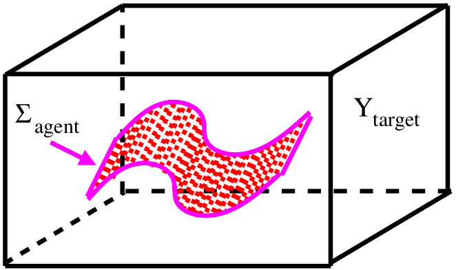
The field theory formulation provides a tool for addressing how the collective would respond to a perturbation to the original inference, and moreover, how estimates on the parameters are correlated over the lattice of agents. If we add a linear source term , we can specify initial conditions for some of the agents. Then, the one-point function will tell us about how the original inference strategy settles towards a preferred value of parameters. The higher point functions tell us about correlations between the guesses of nearby agents.
We can also ask what happens if there is a perturbation to the family of statistical models used by the collective. One might view this as the collective “changing its mind”, or equivalently, reacting to a change in the true distribution. Ideally, such perturbations should not completely destabilize the original inference, though the collective should be capable of altering its original inference. For simplicity, we mainly focus on the case of uniformly weighted agents in flat space.
Surprisingly, the answer is very sensitive to the geometry of the agents. For , a small change in the probability distribution generically destabilizes the original inference, that is, the collective does not reach the same inference. For , these perturbations wash out, and do not change the original inference. When , however, the collective can adjust its inference procedure.
In other words, stable statistical inference selects out two dimensions for the grid of agents. The limiting case where the overall dependence on the number of agents drops out translates to the condition of conformal invariance in the sigma model. As is well known the condition of conformal invariance leads directly to the Einstein field equations for classical gravity. Quantum fluctuations around the background metric arise from fluctuations in the inferred probability distribution. As far as we are aware, this is the first derivation of classical gravity from the condition of stable statistical inference.
The classical description breaks down at small distance in the fitting parameter space. This occurs at a statistical resolution length (in units where ):
| (1.7) |
with the number of sampled events. In physics terms, this sets a cutoff for the target space theory, which we interpret as the string scale associated with the sigma model.
To reach a full string theory, we can make the stronger demand that we sum over all possible arrangements of the agents by coupling the sigma model to two-dimensional gravity. Quantum stability can be ensured by passing to the superstring. Each agent can then be viewed as the endpoint of an open string, that is, a D-instanton, and a collective of D-instantons can build up a string. From this perspective, the condition of stable inference gives an explanation for why a quantum theory of gravity must contain stringlike excitations.
Turning the discussion around, we also apply methods from statistical inference to the study of superstring theory. We ask how well an observer could hope to resolve the internal geometry of a compactified spacetime . A guess by an observer defines a probability distribution which depends on the location of the observer , as well as other fitting parameters which characterize the local profile of the metric. This generates a family of probability distributions, and a corresponding information metric. Calabi-Yau compactifications can be understood in information theoretic terms as generating successively better numerics for a balanced metric (see e.g. [4, 5, 6, 7]). Comparing the true probability distribution with the original guess, we can then quantify the amount of information an agent would gain by adjusting their initial incorrect guess of the internal geometry. We also entertain some more speculative material on potential applications to the AdS/CFT correspondence, as well as Lorentzian signature statistical manifolds.
The rest of this note is organized to reflect the fact that some pieces may be of interest to different readers. In section 2 we briefly review some background on statistical inference and information geometry, and in section 3 we present a sigma model for statistical inference and study some of its properties using results which –though well-known to string theorists– may seem surprising. After this, we focus our attention on applications to the physical superstring. We study the information content of a superstring compactification in section 4, and briefly entertain some more speculative applications in section 5. We conclude in section 6.
2 Statistical Inference and Information Geometry
In this section we review the main concepts from statistical inference and information geometry which we shall use. Excellent resources are the reviews [8, 3].
Given a probability space with measure we would like to define some notion of two probability distributions being nearby. A common choice is the Kullback-Leibler divergence between the true density and a guess :
| (2.1) |
which is also known as the relative entropy. Though it is not a true metric (as it is not symmetric), the Kullback-Leibler divergence is non-negative, and has a simple statistical interpretation as quantifying the amount of information (in the sense of Shannon [9]) an agent would gain by learning the true distribution. One can also introduce the continuum generalization of the Shannon entropy known as the differential entropy, by integrating . This must be treated with more care, because this “entropy” can be negative.
Of course, the Kullback-Leibler divergence is but one way to compare the proximity of distributions. In fact, in the small distance limit, other notions of proximity produce the same notion of distance between distributions. To see this, consider a parametric family of probability densities depending on coordinates of some manifold :
| (2.2) |
which are infinitesimally close to the true distribution. Expanding to second order in then yields the Fisher information metric:
| (2.3) |
with as in equation (1.6).
A central result in information geometry is Chentsov’s theorem [10]. This theorem guarantees that at least in situations where we can sample the true distribution sufficiently often, the infinitesimal form of the distance will eventually converge to the Fisher information metric, that is, equation (2.3). In this sense, the infinitesimal form of statistical inference is relatively insensitive to which finite distance measure between distributions we choose to adopt.
Now, having introduced a metric for the Riemannian manifold , the first inclination of a physicist might be to study geodesic flows with respect to the Levi-Cevita connection . This is certainly possible to do, but it turns out to not be the only natural choice in the case of statistical inference. We can also introduce connections with torsion which are specifically adapted to a fixed choice of affine coordinate system. We can then define another connection via the implicit relation . The use of connections with torsion is quite prevalent in the information geometry literature. This is because one is often concerned with a privileged class of probability distributions, and therefore must adapt an affine coordinate system for this specific distribution. Parallel transport with respect to the Levi-Cevita connection will generically disrupt this coordinate system, so it is common (see e.g. [3]) to label a statistical manifold by the triple .
To illustrate some of the above notions, consider the case of a normal probability distribution for outcomes . The fitting parameters are positions and an overall width:
| (2.4) |
The information metric is:
| (2.5) |
We find it striking that this is also the metric for Euclidean Anti-de Sitter space in dimensions.
2.1 Statistical Mechanics of Statistical Inference
We now review the statistical mechanical interpretation of statistical inference [1, 2]. We start with a probability distribution with density which has generated independent events . The aim is to find a statistical model which comes closest to approximating this distribution. Given two models and we can compute and . The aim is to pick the model with the higher conditional probability.
Suppose our agent has made a choice for a parametric family of models with continuous fitting parameters . Using Bayes’ rule, the Bayesian posterior probability is:
| (2.6) |
where is some choice of weighting scheme for the parameters . Here, is the prior probability for the family of models , and is the probability of the event set .
Now, the key step is that in the limit where the agent has sampled a large number of independent events, the law of large numbers implies that approaches (in the almost sure sense) [1, 2]:
| (2.7) |
where is the Kullback-Leibler divergence and is the differential entropy:
| (2.8) |
In other words, in the large limit is a partition function:
| (2.9) |
This provides a statistical mechanical interpretation for statistical inference [1, 2]. The number of sampled events corresponds to the inverse temperature, and the Kullback-Leibler divergence is an energy. Up to a -independent shift, the quantity can be repackaged as indicating the interaction between the guess and “statistical defects”. Moreover, just as in thermodynamics, there is a competition between minimizing the energy, and maximizing the entropy. This corresponds to balancing the interests of minimizing the distance between and , and on the other hand, the possibility of probing more nearby configurations. In the “quenched approximation” to the partition function, we can basically drop the background value of . Indeed, we shall mostly neglect this contribution in our considerations.
If we assume that the probability density is nearby the true density in the sense of equation (2.2), we can further approximate the energy as:
| (2.10) |
Finally, in [1, 2] additional care is paid to the choice of a weighting function , where it is argued that the natural choice for a uniform sampling of models is the Jeffrey’s prior, corresponding to the choice . The integration measure is then parametrization invariant. Of course, depending on the prior information, one might make different choices.
3 Field Theory for Statistical Inference
In this section we turn to the core of our analysis, where we generalize [1, 2] to a collective of agents. Now, whereas a single agent must settle for one inference scheme, a collective can sweep out a bigger set of guesses. What we show is that the pooled posterior probability of the collective fitting the data is the partition function of a non-linear sigma model. We include some additional heuristic background on such field theories since some aspects may be unfamiliar to the reader.
We define a collective of agents as a set of nearby statistical models . Each agent draws events from the true distribution for . The models are assumed to be nearby in the sense that they each depend on parameters for some guess distribution. In other words, we get sets of fitting parameters , where each itself specifies fitting parameters. Restoring all indices, we label each such parameter as for and . To be part of the collective, we assume that the fitting parameters of agents are correlated. The specific type of correlation between agents is taken as part of the defining data of the collective.
For each agent, we have the Bayesian posterior probability:
| (3.1) |
where is the energy for each agent, and is the differential entropy of the true distribution. In principle, the prior probability of each agent’s guess, as well as their weighting schemes could vary from agent to agent.
Our interest is not in the success of any individual agent, but instead the full collective. What we want to study is the pooled posterior probability of the collective as a whole to reach some inference. Along these lines, we introduce the pooled posterior probability of the collective:
| (3.2) |
When the context is clear, we shall denote this by . This definition reflects the assumption that although the agents of the collective are required to make nearby guesses, they are otherwise independent. Given two collectives and each composed of agents, our aim will be to select the collective with the higher pooled posterior probability. We can also compare the success of a collective to that of a single agent by computing .
3.1 Lattice Approximation
To give the problem some more structure, we shall now assume that the agents are aligned along a -dimensional grid, which is assumed to be a lattice approximation to some -dimensional manifold . For each choice of point in the lattice approximation to , we can pick a value for . In other words, we build up an approximation to the map:
| (3.3) |
In this case, the collective is defined by the condition that nearby fluctuations in the agent space are correlated as:
| (3.4) |
with summation on the indices implicit. In this case, performing the integral then sweeps out a range of possible maps.
Let us illustrate the lattice approximation for . We introduce a collection of unit normalized vectors ,…, . We span a grid with the linear combinations where is a small parameter and are integers. A lattice derivative in the direction corresponds to:
| (3.5) |
for and . Discretized integration corresponds to the substitution:
| (3.6) |
where we have introduced a notion of distance between neighboring agents via the metric on the agent space. To focus on the essential points, we shall typically take to be a constant matrix. Much of what we say generalizes to a broader class of agent space metrics.
In practice, the space will typically have finite volume. The lattice approximation therefore amounts to fixing some small unit cell of size , and arranging these cells to produce the total volume of :
| (3.7) |
The continuum limit corresponds to sending and with Vol held fixed.
We would now like to argue that inference of the collective defines a -dimensional quantum field theory of a very particular type. Since we are assuming the family of guesses are close to the true distribution, we can expand the energy at a point as in equation (2.10). This defines a pullback of the metric on to a metric on :
| (3.8) |
where denotes the matrix inverse of . In the limit of a large number of agents, the lattice approximation tends to:
| (3.9) |
up to a common overall constant normalization factor. Here, the measure factor is a heuristic instruction to integrate over all possible maps . The contribution is the kinetic term for a non-linear sigma model:
| (3.10) |
The kinetic energy defines a sum over the infinitesimal Kullback-Leibler divergences for all of the agents, measuring the proximity of the collective to the true distribution. This provides a first indication of how a collective inference might differ from an individual inference: Whereas individual agents might produce sharp jumps in making different inferences, the collective might instead smooth these out to only gradual changes across the entire agent space. In statistical terms, the collective gains more by exploring many nearby options than by trying to minimize the Kullback-Leibler divergence of a single agent.
The other terms of equation (3.2) also define natural objects in this quantum field theory. For example, the agent dependent weighting factor lifts to a possibly position dependent potential energy:
| (3.11) |
where:
| (3.12) |
and similar considerations apply for the position dependent potential energy on agent space:
| (3.13) |
Again, this makes intuitive sense; a choice of weighting scheme dictates where the statistical inference procedure may be attracted. A position dependent potential term means not all agents are weighted equally. In most uniform weighting schemes one is essentially demanding Lorentz invariance of the continuum theory.
Assembling all of the pieces and integrating over the class of all possible maps, i.e. choices of , we have arrived at the path integral formulation of a non-linear sigma model. Statistical inference of the collective determines a quantum field theory!
It is convenient to adhere to standard practice in field theory by rescaling the fields to eliminate the explicit factors of appearing in our continuum theory integrals. Doing so, we arrive at the final form of the partition function for a non-linear sigma model:
| (3.14) |
where:
| (3.15) |
in the obvious notation. This is the action in Euclidean dimensions for a non-linear sigma model which has been deformed by a field and position dependent potential energy. Here, we have adjusted the measure of the path integral by a factor of so that refers to the Jeffrey’s prior.
A More Formal Derivation
At various stages in our derivation, we took some heuristic liberties. In this subsection we give a more formal derivation. We can view the agents as a single “meta-agent” which has sampled the probability space . We label an outcome from this probability space as the -tuple . The entire set of fitting parameters is then for . The index indicates both an agent as well as a fitting index . In this formalism, the true distribution sampled by the agents of the collective is simply the product:
| (3.16) |
and the parametric family of models used by the collective can be summarized as . The inference scheme of the collective can be viewed as a single meta-agent drawing events from the true distribution . Each event is itself a -tuple of events drawn from the . Denote this set of events by , and let denote the family of models parameterized by the . Then, we can re-write the pooled posterior probability as:
| (3.17) |
In physics terms, the integration measure is simply that used in the path integral.
To define the notion of a grid, we will actually need to enlarge the fitting parameter space to copies of the meta-parameters. So, we label these fitting variables as , where runs over the dimensions of the grid. To enforce the condition that there are no additional degrees of freedom in the fit, we assume that includes a delta function constraint which imposes the condition .
Now, using the law of large numbers to convert into a Boltzmann factor, we can express the conditional probability as:
| (3.18) |
where is the Fisher information metric for the meta-agent:
| (3.19) |
The energy functional can now be viewed as a matrix product in three different spaces. First, there is the sum over , i.e. the different directions of the grid. Second, there is the meta index which splits up as a choice of agent, and a direction in the fitting parameter space. The simplest possibility which is generated by product distributions is that simply factors as:
| (3.20) |
that is, we sum over , , and integrate over in the agent space. The variation:
| (3.21) |
is simply a particular matrix multiplication operation on the . It is well-defined since we are imposing the constraint that . Hence, we can perform a sum over all the agents in the expression . The result is simply the kinetic term for the non-linear sigma model:
| (3.22) |
where measures the infinitesimal proximity between models, and is the proximity between the agents, as defined by the more general information metric in equation (3.19). Similar considerations apply for the other contributions to the partition function. This leads us back to our expression for the partition function in equation (3.14).
3.2 Correlations and Inferences
We can now repurpose many of the methods used in quantum field theory to study inference schemes of the collective. If we perform the analytic continuation to a Lorentzian signature agent grid, we can treat the system as a -dimensional grid of agents which updates along a grid of time steps.
We specify boundary conditions for the system by introducing a position dependent chemical potential for the parameters. This is a source in the field theory:
| (3.23) |
Correlation functions of the quantum field theory are given by functional derivatives with respect to the source:
| (3.24) |
Of particular interest is the behavior of the one-point function in some asymptotic limit of the agent parameters . In Euclidean signature this tells us about the boundary behavior of the collective, and in Lorentzian signature, it tells us about the late time behavior of the collective.
It is important to stress that our formalism implicitly assumes we are already close to the true distribution. In other words, we assume that all fluctuations in the fitting parameters are small.
In some cases the field theory will admit a semi-classical approximation, corresponding to expansion around a saddle point of . Performing a functional derivative of with respect to yields a classical evolution equation for the ’s:
| (3.25) |
or,
| (3.26) |
We view and the independent part of as specifying a prior on the guess in the statistical parameter space.
As an illustrative example, consider the case where our guess is a single centered normal distribution of fixed width. The information metric is the flat space metric on , with entries proportional to the identity matrix:
| (3.27) |
Let us further suppose that our initial weighting scheme by specifies a quadratic potential . This corresponds to an initial weighting scheme by a Gaussian of width centered on . All together, this describes a free quantum field theory with a mass term. The presence of the mass term means that eventually the configuration will aim to roll towards .
How it gets there is another matter, which is sensitive to the number of dimensions for the agent space. In , long range correlations between agents die off sufficiently quickly that we can use a semi-classical evolution equation. In , more care is needed in the nearly massless limit.
To further illustrate the field theory perspective, let us consider another example, given by the sum of two normal distributions for outcomes :
| (3.28) |
We hold fixed the width , but vary the parameters and , so our statistical manifold is parameterized by the product . In the limit where , we can evaluate the leading order form of the information metric:
| (3.29) |
When , the information metric collapses to a rank one constant matrix. In the field theory, this means the mode does not propagate, leaving only the center of mass degree of freedom . The statistical interpretation is analogous: In the limit where the two peaks coincide, we do equally well to fit the distribution to a single Gaussian; one of the degrees of freedom has become irrelevant.
3.3 Stability Under Perturbations
In this subsection we study the stability of the collective against perturbations. For simplicity, we shall assume that the potential energy only depends on implicitly through its dependence on . We shall also assume that the agent space is equipped with a flat metric.
Our aim will be study the growth / dissipation of perturbations to the original inference scheme as the number of agents becomes very large. Alternatively, this can be viewed as asking what happens when the collective “changes its mind” by perturbing its initial family of guesses.
We are particularly interested in stable inference schemes. On the one hand, this means that such perturbations should not drastically change the original inference. On the other hand, this also means that the collective should be capable of changing its original inference.
The theoretical tool we use to address the response to perturbations of the collective is the renormalization group of the field theory. Roughly speaking, we can partition the original agent space into a set of ever cruder averages over nearest neighbors. The renormalization group equations track the response of perturbations as we perform this averaging procedure. Letting denote a perturbation of either the background metric or the potential , we ask whether is amplified or suppressed as the number of agents grows. In field theory terms, the scaling behavior defines a beta function:
| (3.30) |
Stability under perturbations translates to the condition that we arrive at an interacting conformal fixed point, so in particular we require .33 3 For earlier work on the potential relevance of scale invariance in certain inference problems such as applications to perception, see for example [11, 12], as well as [13] for a holographic interpretation.
Rather than delve into a detailed analysis, we will instead present some heuristic intuition for the different behavior couplings can exhibit by using –basically classical– dimensional analysis arguments. The statements we make receive various quantum corrections, which we shall basically gloss over, except in subsection 3.4 when we treat the special case .
Since we have introduced a length scale which indicates the proximity between agents on , scaling with respect to this parameter will show up when we coarse grain the approximation on the agents. In particular, this dimensionful scale will also be related to the scaling behavior of the fitting parameters . To fix the overall scaling dimension, we first note that the exponential is only well-defined provided , the action of the sigma model is dimensionless. Now, since the integral over the agent space defines a -dimensional volume Vol, it follows that the ’s must have appropriate dependence to make dimensionless. For example, in the action:
| (3.31) |
must scale as for to be dimensionless. Since each derivative specifies a factor of (c.f. equation 3.5), it follows that classically scales as . More generally, we can consider the case of a -dimensional agent space. By expanding around some constant value, we learn that the classical scaling of is .
Now, we are going to use this same dimensional analysis argument to compute the scaling behavior of perturbations to the original field theory. Though we do not do so here, one can give more rigorous versions of these arguments.
Consider first the possibility that the collective decides on a different inference scheme. This corresponds to a perturbation , which will in turn show up as a change to the original information metric. In the sigma model, we track this perturbation by expanding near some point . Letting denote small variations, we can expand the kinetic term around this value:44 4 Actually, if we work with Riemann normal coordinates the variations begin at quadratic order, with proportional to the Riemann tensor.
| (3.32) |
Since scales in the same way as , we can work out the scaling behavior of each of these perturbations as a function of length. Each subsequent perturbation involves additional factors of , so we have . To compute the scaling behavior of these perturbations with respect to , we recall that the volume of the agent space Vol is being held fixed throughout the analysis. Hence, we can solve for in terms of , which implies each such perturbation scales with the number of agents as:
| (3.33) |
In other words, in the limit, these perturbations die off for , while for , these terms alter the long distance behavior of the field theory. For , such perturbations could potentially be marginal.
The interpretation in the statistical setting is quite intriguing: If we start with a given sigma model of statistical inference, we can ask whether the collective will alter its inference significantly if it makes a change to its original guessing strategy. These perturbations will show up as variations of the information metric.
When , the collective simply retains its original inference, the inertia of the group prevents changes.
When , on the other hand, we see that each small perturbation has a dramatic effect on the original inference.
When , we see another possibility, namely that such perturbations could be marginal, and that the collective can smoothly change its inference scheme. This is a special feature of two-dimensional non-linear sigma models.
For completeness, we perform a similar analysis in the case of a change to the weighting scheme, i.e. the potential energy . We consider a perturbation to of the form:
| (3.34) |
which will show up as a potential term of order in the field theory. Repeating the same scaling analysis, one learns that scales with the number of agents as:
| (3.35) |
with as in equation (3.33). Thus, for , we see that a change with will not alter the original inference. However, for low enough degree ’s, the weighting scheme can significantly alter the outcome. Similarly, we see that for , such perturbations are always significant.
3.4 Two-Dimensional Case
Summarizing the previous subsection, we have seen that the case of a two-dimensional agent space is rather special. In this subsection we discuss in more detail the conditions for stable inference in two dimensions. From the perspective of string theory, our discussion of conformal invariance and the appearance of gravity is not new. How we managed to arrive here is another story.
We restrict our attention to the well-motivated subcase corresponding to the Jeffrey’s prior. To begin, we also assume a flat agent space metric .
Renormalization of 2d non-linear sigma models has received enormous attention in the string theory literature. See for example [14, 15, 16] and [17] for a review. In two dimensions there is an additional coupling we can write which also has an information theoretic interpretation:
| (3.36) |
The coupling is an additional anti-symmetric tensor on the target space, and is a constant anti-symmetric tensor in the two-dimensional geometry. In the target space, a background value of specifies a notion of torsion, that is, parallel transport with respect to a connection distinct from the Levi-Cevita connection on . This recovers the use of connections with torsion in information geometry discussed in section 2. Readers familiar with string theory will note that we have omitted a factor of the dilaton coupling. This is because the collective works with respect to a fixed and flat agent space metric.
Assuming the response of the collective is independent of the number of agents, we arrive at the condition of conformal invariance for the 2d sigma model. Treating the values of , as background fields of the target space geometry, conformal invariance implies the conditions (see e.g. [17] for a review):
| (3.37) |
where is the Ricci tensor for the information metric, is the Ricci scalar, . Here we have not written subleading higher derivative corrections, which are suppressed by powers of . Equations (3.37) are the Einstein field equations, coupled to a background flux. As is well-known, they are reproduced by a principle of least action on the -dimensional target:
| (3.38) |
Adding an explicit source of stress energy to the Einstein equations corresponds to exposing the collective to a new source of information. In the semi-classical approximation, we can also identify the graviton as a fluctuation in the information metric, that is, a fluctuation in the family of probability distributions adopted by the collective.55 5 One might speculate on a connection to entropic gravity [18], though we do not do so here.
From these considerations alone, however, Newton’s constant is simply a parameter of the theory. Indeed, our considerations here are weaker than what would follow from a full string theory. In particular, the absence of a dilaton equation of motion means that we cannot fix Newton’s constant, and further, that the number of fitting parameters is subject to no constraint. The price we pay for this is that our description will break down at short distances on , namely “the string scale”:
| (3.39) |
This reflects the underlying statistics from the number of sampled of events, so we typically do not demand more.
If we do demand that our description makes sense below the resolution scale of the statistics, we need the machinery of string theory. We get a string theory by summing over all arrangements of the agents, that is, by coupling our sigma model to 2d gravity on the worldsheet. Then, the dilaton will automatically appear, and will couple to the worldsheet curvature via the term . The string frame metric is then the information metric. Stable inference schemes of the collective then yield the stronger condition of Weyl invariance on a curved worldsheet. We can eliminate tachyonic modes by passing to the superstring. Indeed, there is a natural extension of our analysis to the case where the agent space is a supermanifold.
4 Information and Compactification
In this section we switch gears, applying information geometry to study compactifications of the physical superstring. There are two interlinked questions we wish to study. First, we want to know whether information metrics produce accurate approximations to metrics of compactification manifolds. Second, we want to know how much information an observer would gain by correcting an incorrect guess of the internal geometry.66 6 One of the original motivations for this note was to understand in information theoretic terms the non-commutative geometry of F(uzz) theory [19], as well as the evidence presented in [20, 21, 22] for the interplay between fuzzy UV cutoffs and an emergent gravitational sector.
We shall assume a compactification of the physical superstring of the form , where is a Calabi-Yau threefold. We expect that most of our considerations extend to other Kähler threefolds, as can occur in various F-theory compactifications.
Since is Calabi-Yau, and therefore a Kähler manifold, its metric is locally controlled by a Kähler potential . We can split up the local coordinates into holomorphic and anti-holomorphic coordinates and . The metric is then:
| (4.1) |
Compare this to the Fisher information metric. Assuming is our statistical manifold of parameters for some probability space , we get distributions , and an information metric on :
| (4.2) |
Making the further assumption that only the mixed holomorphic and anti-holomorphic terms contribute, we see that defines a stochastic generalization of the Kähler potential.
To complete the circle of ideas, we need to find a collection of ’s such that is a good approximation to . Assuming that this can be done, we can check the inference abilities of an observer by comparing the true distribution to a nearby guess. This provides a measure of how well an observer can deduce the local geography of a compactification.
4.1 Construction of Metrics
Our strategy for constructing a family of information metrics will be to initially take , and an ambient target space . Starting from this, we show how to reduce to an information metric on , and by embedding a Calabi-Yau in such a projective space, we shall produce a numerical approximation for a Calabi-Yau metric.
We first construct a family of information metrics on using the Gaussian:
| (4.3) |
where denote holomorphic coordinates for , denote holomorphic coordinates of the parameter manifold , and is an invertible Hermitian matrix with positive eigenvalues. The non-vanishing entries of the information metric:
| (4.4) |
are generated by the Kähler potential:
| (4.5) |
Viewing as the guess of where a probe is located inside the geometry, we can also adjust the parameters which specify the width of the guess. This leads to a much larger parameter space, with information metric:
| (4.6) |
To construct information metrics on other parameter spaces, we restrict the range of parameters of . For example, we can define a sphere by restriction on the parameter manifold to the fixed locus:
| (4.7) |
The restriction to this locus (holding fixed) yields a pullback of the metric on to . By a similar token, we can also pull back the probability density on to . Here, we must be careful to respect the condition that is a density, and not a scalar of . The restriction to now follows by reducing along the fiber of the Hopf fibration , so we produce an information metric on which agrees with the Fubini-Study metric generated by the Kähler potential:
| (4.8) |
with the now treated as homogeneous coordinates of .
A similar construction also applies to the case where is Calabi-Yau. The idea is to fix an ample line bundle over . Since is ample, the space of sections defines an embedding of into the projective space :
| (4.9) |
This is an embedding to projective space since the cannot all simultaneously vanish. One can view the Calabi-Yau as defined by a set of polynomial relations amongst the . This need not be a complete intersection, since there could be relations amongst the relations (syzygies). Given the Fubini-Study Kähler form on , we get a form on via the pullback . Hence, each choice of Hermitian matrix defines a candidate metric for . We view this choice as the inference strategy of a given agent.
To produce a best approximation, we follow the numerical procedure for constructing balanced Calabi-Yau metrics used in [6, 7]. The optimal choice is fixed under the T-map (see [4, 7]):
| (4.10) |
For a Calabi-Yau, the fixed point exists. Now, although this is not yet the form of the Calabi-Yau threefold, repeating the construction for sufficiently high degree powers of the line bundle defines a sequence of balanced metrics which eventually converge to the Kähler form of the Calabi-Yau metric (see [4, 5]):
| (4.11) |
as . Observe that in this construction, the Chern class , i.e. it picks a ray in the Kähler cone which is compatible with geometric quantization of the Calabi-Yau [4].
The statistical inference interpretation should be clear. We can make a guess both as to the location of the observer, as well as the local profile of the Calabi-Yau metric, via . A sequence of improved guesses, both in the choice of location, and Hermitian metric eventually converge on an adequate approximation of the internal geometry.
To illustrate how much an observer can learn by adjusting an incorrect guess of the local geometry, let us return to the case of distributions on the ambient space . Similar comments apply for all of the pullback / restriction maps. Suppose that the true distribution of the observer is centered at some point , and that it is designated by a choice of Hermitian matrix . Then, if our observer makes an incorrect guess given by some other choice of and , the amount of information it would gain by adjusting its choice is the Kullback-Leibler divergence:
| (4.12) |
The observer learns both by locating its position, and its width correctly. The supergravity limit of the compactification corresponds to a sharply localized observer with , and the small volume limit corresponds to sending . In both cases, the observer learns much by adjusting its width. By the same token, once the observer get close to the true distribution, it ceases to learn very much about the internal geometry. In this sense, though there is only one true distribution, a nearby guess is “good enough”.
4.2 Quantum Interpretation
The information geometry of a Calabi-Yau is also closely connected with tiling a non-commutative deformation of the geometry with nearly pointlike branes, as in F(uzz) theory [19]. In this subsection we show that the Hilbert space of fuzzy points for induces a family of quantum information metrics for the Calabi-Yau.
Let us begin by briefly reviewing some background on quantum information metrics. Given a Hilbert space and density matrix which depends on continuous parameters , we can introduce a quantum analogue of the Fisher information metric, known as the Helstrom / Bures metric (see [23, 24]):
| (4.13) |
where we have chosen a convenient normalization convention. Here, is implicitly defined via:
| (4.14) |
Extending the cases treated in [19], we realize a non-commutative Calabi-Yau threefold by first constructing non-commutative . Imposing a level constraint and additional holomorphic constraints leads to non-commutative geometry on subspaces. Since the restriction maps of the previous section were specified by holomorphic conditions, we can carry over our construction to the fuzzy case.
In more detail, we first construct the fuzzy Hilbert space of points for . Introduce harmonic oscillators , which are subject to the commutators:
| (4.15) |
Next, introduce a vacuum state such that . We then build up a Fock space of fuzzy points for by acting with creation operators on . Denote this Hilbert space of states by . For each , introduce a coherent state:
| (4.16) | ||||
| (4.17) |
These are normalized states, and form an overcomplete basis for . We can introduce a further grading of by the operator:
| (4.18) |
We refer to an eigenspace of at eigenvalue as the Hilbert space of points for fuzzy at radius . In what follows we work at large radius. This is the fuzzy analogue of the Kähler quotient constraint:
| (4.19) |
The fuzzy Hilbert space of points for a Calabi-Yau is obtained by restricting to states of annihilated by the holomorphic relations of the commutative geometry:
| (4.20) |
where the are themselves possibly subject to further relations (syzygies).
We now produce a quantum information metric for , and pull this back to via the embedding . We begin with a construction of the Fubini-Study metric on by working with the density matrix for the family of pure states:
| (4.21) |
Observe that since , we have .
Thus, to compute the quantum information metric it is enough to consider the variation of as we change , subject to the variation of the Kähler quotient constraint in line (4.19):
| (4.22) |
To leading order in , the normalization of remains fixed because . Hence,
| (4.23) |
where we have introduced the unnormalized states:
| (4.24) |
Note that the transversality condition of line (4.22) implies . The quantum information metric therefore reduces to:
| (4.25) |
so we recover the Fubini-Study metric on due to the Kähler quotient constraint of line (4.19). Returning to our discussion in subsection 4.1, the pullback to then gives an approximation for the Calabi-Yau metric.
5 Speculative Remarks
In this section we entertain some speculative remarks on other possible uses of information geometry in the study of superstring theory. We take an agent to be a D-instanton, that is, the endpoint of an open string. The D-instanton comes with a local position, and possibly other parameters such as its width, when it dissolves as flux in another brane. The natural choice of in the supersymmetric setting is simply the moduli space of the brane.
5.1 Simplistic Holography
One of the most direct ways to probe the AdS/CFT correspondence is via D-instantons [25, 26, 27, 28]. Indeed, the instanton density in Yang-Mills theory defines an unnormalized probability distribution, and a corresponding information metric [29] which provides another way to interpret the AdS/CFT correspondence [30].
Rather than delve into the details of the instanton moduli for a specific gauge theory, we instead try a more simplistic approach. Given a large stack of D3-branes filling in a consistent 10D geometry, we consider a D-instanton inside the worldvolume of the stack. We can view the D-instanton as independently sampling the D3-branes many times with the large number of D-1 / D3 strings. Assuming finite mean and variance for this sampling, the central limit theorem allows us to approximate the profile of the D-instanton by a Gaussian on . In physical terms, it is actually most natural to use an unnormalized parametric family of such distributions:
| (5.1) |
The mean of the distribution tells us the average position of the D-instanton, and the width sets a resolution length. The information metric for this distribution is 5D Euclidean AdS space of radius :
| (5.2) |
Similar considerations hold in other dimensions. Observe that our discussion only required a large number of strings to sample the stack of D3-branes, and is otherwise insensitive to the details of the gauge theory. It would be very interesting to see whether a simplistic treatment along the lines presented here could also reproduce the factor of the holographic dual.
5.2 Lorentzian Signature Statistics
Much of our focus in this work has been on the inference abilities of a collective of agents probing a Riemannian manifold. For applications to physics, one should eventually return to Lorentzian signature. This opens up some new possibilities as well as challenges from the perspective of information geometry.
To illustrate the main issue, consider again the normal distribution, but now in Lorentzian signature. We can of course simply write down a formal Gaussian profile on :
| (5.3) |
via the formal analytic continuation from (and taking the norm). Since analytic continuation of a D-instanton to Lorentzian signature defines a tunneling event, we take the unbounded behavior of to mean that while the agent eventually settles on a choice of for spatial directions, it continues to move forward in the temporal direction.
Yet another new feature of Lorentzian signature spacetimes is the possible existence of null vectors. In information theoretic terms, this means nothing is learned by moving along the null direction. It would be interesting to study the consequences for black hole event horizons and cosmological horizons.
A temporal direction in statistical inference also shows up from sequential updating of the events received by an agent. We can then drop the distinction between and by using a lattice approximation for a -dimensional field theory. It would be interesting to connect this to the field theory interpretation of Bayesian updating in [31].
6 Conclusions
In this note we have studied the interplay between statistical inference and string theory. We have shown that when a large number of agents form a collective of nearby guesses, the pooled posterior probability of an accurate inference by the collective is the partition function of a non-linear sigma model. Quite surprisingly, stability of the inference scheme against perturbations requires the collective to arrange along a two-dimensional grid. Using the well-known fact that the Einstein field equations follow from the condition of conformal invariance in 2d non-linear sigma models, we found classical gravity emerge from the condition of stable statistical inference. We have also taken some preliminary steps in applying methods from information geometry in the study of the physical superstring.
Developing more practical applications of this formalism would be quite interesting. For example, one might try to simulate a dynamical updating strategy for a collective of agents.
Much of our discussion generalizes to the quantum setting, with a quantum information metric for the non-linear sigma model. It would be interesting to further study the interpretation in the context of both quantum statistical inference and string theory.
Finally, we find it rather remarkable that stable computations by a collective requires a two-dimensional worldsheet, and moreover, that this yields a theory of gravity. It would be exciting to further develop an information theoretic formulation of such “computables”.
Acknowledgements
We especially thank J.J. Heckman Sr., D. Krohn and A. Murugan for helpful discussions and comments on an earlier draft. We also thank L.B. Anderson, Y.-T. Chien, S. Detournay and D. Farhi for helpful discussions, and V. Balasubramanian for encouragement. The work of JJH is supported by NSF grant PHY-1067976.
References
- [1] V. Balasubramanian, “A Geometric Formulation of Occam’s Razor For Inference of Parametric Distributions,” arXiv:adap-org/9601001.
- [2] V. Balasubramanian, “Statistical Inference, Occam’s Razor and Statistical Mechanics on the Space of Probability Distributions,” Neural Comp. 9(2) (1997) 349–368, arXiv:cond-mat/9601030.
- [3] S.-I. Amari and H. Nagaoka, Methods of Information Geometry, vol. 191. Translations of Mathematical Monographs; American Mathematical Society and Oxford University Press, Providence, RI, 2000.
- [4] G. Tian, “On a set of polarized Kähler metrics on algebraic manifolds,” J. Diff. Geom. 32 (1990) 99–130.
- [5] S. Zelditch, “Szego kernels and a theorem of Tian,” Int. Math. Res. Notices 6 (1998) 317–331.
- [6] S. D. Donaldson, “Some numerical results in complex differential geometry,” arXiv:math.DG/0512625.
- [7] M. R. Douglas, R. L. Karp, S. Lukic, and R. Reinbacher, “Numerical Calabi-Yau metrics,” J. Math. Phys. 49 (2008) 032302, arXiv:hep-th/0612075.
- [8] T. M. Cover and J. A. Thomas, Elements of Information Theory. Wiley, New York, NY, 1991.
- [9] C. E. Shannon, “A Mathematical Theory of Communication,” Bell Syst. Tech. J. 27 (1948) 379–423.
- [10] N. N. Chentsov, Statistical Decision Rules and Optimal Inference. Translations of Mathematical Monographs; American Mathematical Society, Providence, RI, 1982.
- [11] W. Bialek and A. Zee, “Statistical Mechanics and Invariant Perception,” Phys. Rev. Lett. 58 (1987) 741.
- [12] W. Bialek and A. Zee, “Understanding the Efficiency of Human Perception,” Phys. Rev. Lett. 61 (1988) 1512.
- [13] Y. Nakayama, “Gravity Dual for a Model of Perception,” Ann. Phys. 326 (2011) 2–14, arXiv:1003.5729 [hep-th].
- [14] D. H. Friedan, “Nonlinear Models in Dimensions,” Ann. Phys. 163 (1985) 318.
- [15] L. Alvarez-Gaume, D. Z. Freedman, and S. Mukhi, “The Background Field Method and the Ultraviolet Structure of the Supersymmetric Nonlinear Sigma Model,” Ann. Phys. 134 (1981) 85.
- [16] C. G. Callan Jr., E. Martinec, M. Perry, and D. Friedan, “Strings in Background Fields,” Nucl. Phys. B262 (1985) 593.
- [17] C. G. Callan Jr. and L. Thorlacius, “Sigma Models and String Theory,” Providence 1988, Proc. of the Theor. Adv. Study Inst. in Elem. Part. Physics: Particles, Strings and Supernovae 2 (1989) 795–878.
- [18] E. P. Verlinde, “On the Origin of Gravity and the Laws of Newton,” JHEP 1104 (2011) 029, arXiv:1001.0785 [hep-th].
- [19] J. J. Heckman and H. Verlinde, “Evidence for F(uzz) Theory,” JHEP 01 (2011) 044, arXiv:1005.3033 [hep-th].
- [20] J. J. Heckman and H. Verlinde, “Super Yang-Mills Theory as a Twistor Matrix Model,” arXiv:1104.2605 [hep-th].
- [21] J. J. Heckman and H. Verlinde, “Gravity Amplitudes from a Gaussian Matrix Model,” arXiv:1112.5209 [hep-th].
- [22] J. J. Heckman and H. Verlinde, “Instantons, Twistors, and Emergent Gravity,” arXiv:1112.5210 [hep-th].
- [23] C. W. Helstrom, “Minimum mean-squared error of estimates in quantum statistics,” Phys. Lett. A25 (1967) 101–102.
- [24] D. Bures, “An Extension of Kakutani’s Theorem on Infinite Product Measures to the Tensor Product of Semifinite -Algebras,” Trans. Am. Math. Soc. 135 (1969) 199–212.
- [25] T. Banks and M. B. Green, “Non-perturbative Effects in String Theory SUSY Yang-Mills,” JHEP 9805 (1998) 002, arXiv:hep-th/9804170.
- [26] M. Bianchi, M. B. Green, S. Kovacs, and G. Rossi, “Instantons in supersymmetric Yang-Mills and D-instantons in IIB superstring theory,” JHEP 9808 (1998) 013, arXiv:hep-th/9807033.
- [27] N. Dorey, T. J. Hollowood, V. V. Khoze, M. P. Mattis, and S. Vandoren, “Multi-Instantons and Maldacena’s Conjecture,” JHEP 9906 (1999) 023, arXiv:hep-th/9810243.
- [28] N. Dorey, T. J. Hollowood, V. V. Khoze, M. P. Mattis, and S. Vandoren, “Multi-Instanton Calculus and the AdS / CFT Correspondence in Superconformal Field Theory,” Nucl. Phys. B552 (1999) 88–168, arXiv:hep-th/9901128.
- [29] N. J. Hitchin, The Geometry and Topology of Moduli Spaces, in Global Geometry and Mathematical Physics, vol. 1451. Springer, Heidelberg, 1988.
- [30] M. Blau, K. Narain, and G. Thompson, “Instantons, the Information Metric, and the AdS / CFT Correspondence,” arXiv:hep-th/0108122.
- [31] W. Bialek, C. G. Callan Jr., and S. P. Strong, “Field Theories for Learning Probability Distributions,” Phys. Rev. Lett. 77 (1996) 4693–4697, arXiv:cond-mat/9607180.