Estimating the parameters of globular cluster M 30 (NGC 7099) from time-series photometry,Thanks: The full light curves presented in this paper (Table 2) are only available in electronic form at the Centre de données astronomiques de Strasbourg (CDS) via anonymous ftp to cdsarc.u-strasbg.fr (130.79.128.5) or via http://cdsweb.u-strasbg.fr/cgi-bin/qcat?J/A+A/Thanks: This work is based on data collected by MiNDSTEp with the Danish 1.54m telescope at the ESO La Silla Observatory.
Abstract
Aims. We present the analysis of 26 nights of and time-series observations from 2011 and 2012 of the globular cluster M 30 (NGC 7099). We used our data to search for variable stars in this cluster and refine the periods of known variables; we then used our variable star light curves to derive values for the cluster’s parameters.
Methods. We used difference image analysis to reduce our data to obtain high-precision light curves of variable stars. We then estimated the cluster parameters by performing a Fourier decomposition of the light curves of RR Lyrae stars for which a good period estimate was possible. We also derive an estimate for the age of the cluster by fitting theoretical isochrones to our colour-magnitude diagram (CMD).
Results. Out of 13 stars previously catalogued as variables, we find that only 4 are bona fide variables. We detect two new RR Lyrae variables, and confirm two additional RR Lyrae candidates from the literature. We also detect four other new variables, including an eclipsing blue straggler system, and an SX Phoenicis star. This amounts to a total number of confirmed variable stars in M 30 of 12. We perform Fourier decomposition of the light curves of the RR Lyrae stars to derive cluster parameters using empirical relations. We find a cluster metallicity , or , and a distance of kpc (using RR0 variables), 8.10 kpc (using one RR1 variable), and kpc (using our SX Phoenicis star detection in M 30). Fitting isochrones to the CMD, we estimate an age of Gyr for M 30.
Key Words.
globular clusters – RR Lyrae – variable stars1 Introduction
In this paper we analyse time-series observations of M 30 (NGC 7099, or C2137-234 in the IAU nomenclature; at J2000.0), one of the most metal-poor globular clusters known, with [Fe/H] -2.1, located at a distance of 8 kpc. This cluster is thought to be of extra-Galactic origin, due to its retrograde orbit (Allen et al. 2006), pointing to its possible accretion by the Milky Way following an encounter with a satellite, as well as its position on the age-metallicity diagram (Forbes & Bridges 2010). M 30 is also thought to have undergone core collapse (Djorgovski & King 1986, e.g.). Here we detect and classify already reported, as well as new variables, and use Fourier decomposition to derive properties of the RR Lyrae stars in this cluster. We then estimate the cluster parameters of M 30, providing us with an independent estimate of the metallicity, distance and age of this cluster, and the first using this method.
2 Observations and reductions
2.1 Observations
We obtained Johnson - and -band data with the Danish Faint Object Spectrograph and Camera (DFOSC) imaging camera at the Danish 1.54m telescope at La Silla in Chile, as part of a programme with the MiNDSTEp consortium. In this programme we are making use of parts of the night when the MiNDSTEp primary-science microlensing observations towards the Galactic Bulge are not possible. The data were obtained in 2011 and 2012, with the 2011 data consisting mostly of -band observations, while the 2012 observations are evenly split between and -band images. The observations are summarised in Table 1.
The imaging CCD is 2147 2101 pixel, with a scale of 0.396 arcsec per pixel, giving a field of view of 14.2 13.9 arcmin2.
| Date | (s) | (s) | ||
|---|---|---|---|---|
| 20110728 | 48 | 10 | ||
| 20110730 | 27 | 15-20 | ||
| 20110803 | 12 | 30 | ||
| 20110804 | 4 | 30 | ||
| 20110806 | 6 | 30 | 14 | 30 |
| 20110809 | 16 | 30-40 | ||
| 20110810 | 1 | 30 | 12 | 30 |
| 20110811 | 12 | 30 | ||
| 20110813 | 6 | 40 | 6 | 30 |
| 20110814 | 10 | 27 | ||
| 20110815 | 6 | 27 | ||
| 20110817 | 6 | 30 | ||
| 20110820 | 16 | 30 | ||
| 20110821 | 16 | 30 | ||
| 20110822 | 7 | 30 | ||
| 20110828 | 8 | 30 | ||
| 20110830 | 6 | 20 | 11 | 30 |
| 20110831 | 16 | 30 | ||
| 20120807 | 37 | 10-20 | 36 | 10-20 |
| 20120810 | 38 | 20 | 38 | 20 |
| 20120811 | 34 | 20 | 41 | 20 |
| 20120819 | 6 | 100 | 4 | 100 |
| 20120820 | 24 | 100 | 22 | 100 |
| 20120821 | 38 | 70-100 | 38 | 70-100 |
| 20120828 | 65 | 50-100 | 65 | 40-50 |
| 20120919 | 40 | 50 | 39 | 40 |
| Total | 301 | 530 |
2.2 Difference image analysis
As in our previous studies of variables in globular clusters (Figuera et al. 2013, Kains et al. 2012; Arellano Ferro et al. 2011), we used the DanDIA11 1 DanDIA is built from the DanIDL library of IDL routines available at http://www.danidl.co.uk pipeline (Bramich et al. 2013; Bramich 2008) to reduce our observations. Using difference image analysis (DIA) enabled us to obtain high-precision photometry for sources within our field of view. The reader is referred to our previous papers (Bramich et al. 2011, e.g.) for a detailed description of the software used; we provide a short summary of the main steps here.
After preprocessing (bias level correction and flat-fielding), our images were blurred with a Gaussian of full-width half-maximum (FWHM) of 3 pixels to avoid undersampling, which is detrimental for determining the kernel in DIA. We then produce a reference image for each filter, stacking images within 10% of the best seeing (), also taking care to avoid including images with many saturated stars. Our reference image consists of 5 stacked images, with a combined exposure time of 100 s, and a FWHM of the point-spread function (PSF) of 3.88 pixels () in , while in the combined exposure time is 80 s from 4 images, and the PSF FWHM is 3.31 pixels (). For each filter, the source positions and reference fluxes were then extracted from the reference image. Images were then registered with the reference, and the reference was convolved with the kernel solution and subtracted from each image, producing a set of difference images. Finally, difference fluxes were measured from each difference image for each source, which we used to construct a set of light curves. In Table 2, we outline the format of the data as it is provided in electronic format with the online version of this paper.
As was noted in previous papers, blending due to the presence of other objects near a source may lead to the reference flux being overestimated. However, non-variable sources are still fully subtracted in the difference images, while variable objects have the amplitude of their variability underestimated if their reference flux is affected by blending, although the shape of their light curve, crucially, will remain unaffected.
| # | Filter | HJD | ||||||||
|---|---|---|---|---|---|---|---|---|---|---|
| () | (mag) | (mag) | (mag) | (ADU s-1) | (ADU s-1) | (ADU s-1) | (ADU s-1) | |||
| V1 | V | 2455779.84508 | 15.360 | 14.475 | 0.004 | 4619.581 | 1.991 | -500.380 | 4.612 | 0.3633 |
| V1 | V | 2455779.84637 | 15.378 | 14.493 | 0.005 | 4619.581 | 1.991 | -455.515 | 4.326 | 0.3185 |
| ⋮ | ⋮ | ⋮ | ⋮ | ⋮ | ⋮ | ⋮ | ⋮ | ⋮ | ⋮ | ⋮ |
| V1 | I | 2455770.83621 | 14.628 | 14.797 | 0.007 | 2843.148 | 3.237 | -68.927 | 2.472 | 0.1593 |
| V1 | I | 2455770.83726 | 14.639 | 14.809 | 0.007 | 2843.148 | 3.237 | -72.977 | 2.461 | 0.1593 |
| ⋮ | ⋮ | ⋮ | ⋮ | ⋮ | ⋮ | ⋮ | ⋮ | ⋮ | ⋮ | ⋮ |
2.3 Photometric calibration
2.3.1 Self-calibration
Although all photometry is affected by systematic errors, steps can be taken to correct for this, in particular with time-series photometry, for which we can carry out a self-calibration of the data (Padmanabhan et al. 2008, e.g.). To do this, we use the method of Bramich & Freudling (2012) to derive magnitude offsets to be applied to each photometric measurement. In practice, this equates to correcting for errors in the fitted value of the photometric scale factor . We find magnitude offsets of the order of 2-3 mmag for most data points, which leads to small difference in the resulting light curves.
2.3.2 Photometric standards
We converted the instrumental magnitudes from our data reduction pipeline to standard Johnson-Kron-Cousins magnitudes by carrying out a linear fit to the relation between our light curve magnitudes and those of the photometric standards of Stetson (2000) in the field of this cluster. The relations, shown in Fig. 1, were used to obtain light curves in standard magnitudes. The standard stars we used cover the full range of colour and magnitude spanned by our CMD. No significant colour term was found and the correlation coefficients are for both filters.


2.4 Astrometry
We used GAIA to perform the astrometry by matching 400 manually picked stars from our reference images with the USNO-B1.0 catalogue of stars (Monet et al. 2003) to derive a linear transformation between our image positions and equatorial coordinates. This means that the coordinates in Table 3 are given at the effective epoch of our reference image, HJD2456151.84. The root mean square (rms) of the residuals from our astrometric fit is 0.23 arcsec, or 0.59 pixels.
| # | RA | DEC |
|---|---|---|
| V1 | 21:40:24.25 | -23:11:46.4 |
| V2 | 21:40:26.44 | -23:12:51.2 |
| V3 | 21:40:15.04 | -23:11:27.9 |
| V4 | 21:39:58.46 | -23:11:43.3 |
| V14 | 21:40:21.10 | -23:11:30.8 |
| V15 | 21:40:21.79 | -23:10:50.1 |
| V16 | 21:40:24.81 | -23:11:48.8 |
| V17 | 21:40:23.66 | -23:11:01.1 |
| V18 | 21:40:21.88 | -23:09:32.4 |
| V19 | 21:40:22.09 | -23:10:43.3 |
| V20 | 21:40:29.83 | -23:11:05.9 |
| V21 | 21:40:47.80 | -23:10:23.9 |
3 Variables in M 30
The first three variables (V1-3) in this cluster were detected by Bailey (1902) using photographic observations made at the Harvard College Station in Arequipa, Peru. V4 was then reported by Rosino (1949), who discovered it using observations of M 30 at 175 epochs, taken between 1946 and 1948 with the 60cm reflecting telescope at the Lojano Astronomical Station, near Bologna in Italy. Rosino also derived periods for V1-3, and refined his period for V1 in a later paper (Rosino 1961). He also noted that V4 did not present the characteristics of an RR Lyrae type variable. He described it as an unusual object, reaching a magnitude of 16.4, remaining at that level for several days, before dropping below the limits of detectability of his photographic plates, i.e. below 18th magnitude. Other light curve features led him to conclude that V4 is a variable of type U Geminorum. This was confirmed in several subsequent publications by Margon & Downes (1983), who obtained spectroscopic evidence that V4 is a cataclysmic variable, and Machin et al. (1991), who also concluded that V4 is most likely a foreground object rather than a cluster member. Pietrukowicz et al. (2008) found a relatively high -band brightness consistent with that assessment, and also noted that V4 has a likely X-ray counterpart detected by the satellite.
Finally, V5-12 were all reported as variable by Terzan (1968), and V13 was reported by Terzan & Rutily (1975), based on photographic observations taken at the 1.52m telescope at ESO between 1972 and 1974.; however they did not publish light curves or periods for any of those variables.
Pietrukowicz & Kaluzny (2004) analysed HST archival data of M 30 and identified two previously unknown RR Lyrae variables, as well as four W UMa-type contact binaries, and an eclipsing close-binary variable with ellipsoidal variations. However, they did not assign those variables catalogue V numbers. Finally, although Smitka & Layden (2010) also studied this cluster, their photometric accuracy is poor due to the cluster’s low altitude for Northern hemisphere observations. They reported three new RR Lyrae star candidates, but did not provide coordinates or a finding chart, so we are not able to cross-correlate our findings with theirs; they also did not assign their variables V numbers.
This amounts to a total of 13 catalogued variables in the cluster, although V4 is now thought to be a foreground object. There are also 7 additional variables reported by Pietrukowicz & Kaluzny (2004), including 2 new RR Lyrae. The present study of M 30 is the first from the Southern hemisphere using CCD photometry, allowing us to carry out a significant update of the variable star population in this cluster.
3.1 Stars that do not show variability
We find that all of the stars V5-V13, reported by Terzan (1968) and Terzan & Rutily (1975) as variables, do not show signs of variability in our data, to within the limits of the rms scatter in our light curves; those limits are given in Table 4. We are also unable to detect variability of the five contact binaries listed by Pietrukowicz & Kaluzny (2004); for most of these, we attribute this to the fact that the variations have amplitudes of mag, for objects with mag, which is very challenging to detect within the rms of our data (Fig. 2). This is especially difficult in the crowded central core, where blending leads to photon noise dominating any intrinsic variability signal. This is also true for the two brightest eclisping variables, which have magnitudes of 17.3 and 17.9 and variation amplitudes of mag. The advent of electron-multiplying CCD (EMCCD) cameras, coupled with DIA, will allow us in the future to obtain high-quality photometry even for stars in the crowded cores of clusters Skottfelt et al. (2013), and to verify the variability status of these objects using ground-based photometry.
| # | rms () | rms () | ||
|---|---|---|---|---|
| V5 | 17.42 | 0.035 | 16.75 | 0.047 |
| V6 | 15.34 | 0.013 | 15.13 | 0.037 |
| V7 | 16.63 | 0.021 | 15.84 | 0.018 |
| V8 | 15.00 | 0.010 | 14.31 | 0.011 |
| V9 | 15.40 | 0.012 | 15.08 | 0.021 |
| V10 | 15.44 | 0.010 | 15.22 | 0.017 |
| V11 | 16.11 | 0.013 | 15.25 | 0.012 |
| V12 | 15.49 | 0.011 | 15.38 | 0.015 |
| V13 | 15.69 | 0.040 | 14.78 | 0.030 |
3.2 Detection of known variables
We recover the first three known RR Lyrae in this cluster (V1-V3) in our data, and calculate periods for each of them, using phase dispersion minimisation (PDM; Stellingwerf 1978) and the “string length" method (Lafler & Kinman 1965). In order to use the longest possible baseline to derive precise periods for these three variables, we used the data from Rosino (1949); these data are published in a table in that paper, and we provide them as an additional resource with the electronic version of this paper22 2 The light curves for V1-V3 from Rosino (1949), as well as the additional data for V1 from Rosino (1961), are available in electronic form at the CDS via anonymous ftp to cdsarc.u-strasbg.fr (130.79.128.5) or via http://cdsweb.u-strasbg.fr/cgi-bin/qcat?J/A+A/. We also used these data to refine our periods by optimising the alignment in phase of that data set with ours; this is highly sensitive to the period, thanks to the baseline of 63 years. We also recovered the two additional RR Lyrae stars reported by Pietrukowicz & Kaluzny (2004) and assign them catalogue numbers V15 and V19, and calculated refined periods for these two stars. We note that V19 is highly blended due to its location in the very centre of the cluster, which explains its peculiar position on the CMD.
We also detect the U Gem variable V4, including some data taken during an outburst period. This star is discussed in more detail in Sec. 3.4.
3.3 Detection of new variables
As in our previous studies, we searched for new variables using three methods. Firstly, we constructed a stacked image consisting of the sum of the absolute values of the deviations of each image from the convolved reference image, divided by the pixel uncertainty , so that
| (1) |
Stars that deviate consistently from the reference image then stand out in this stacked image. Using this method, we discovered 2 new RR Lyrae stars, V14 and V16, both of RR1 type, with V16 also showing signs of amplitude and period modulation due to Blazhko effects or non-radial pulsation (see Sec. 3.4). Secondly, we inspected the light curves of objects which stand out on a plot of root mean square magnitude deviation versus mean magnitude, shown in Fig. 2.
Finally, we also searched for variables by conducting a period search for all our light curves using the string length method, and computing the ratio of the string length for the best- to that of the worst-fit periods, with the smallest ratios expected for true periodic variations. We inspected visually all of the light curves of stars with , where the threshold value of 0.55 was chosen by inspecting the distribution of (see Fig. 3). Using this method, we discovered V17, V18, V20 and V21.
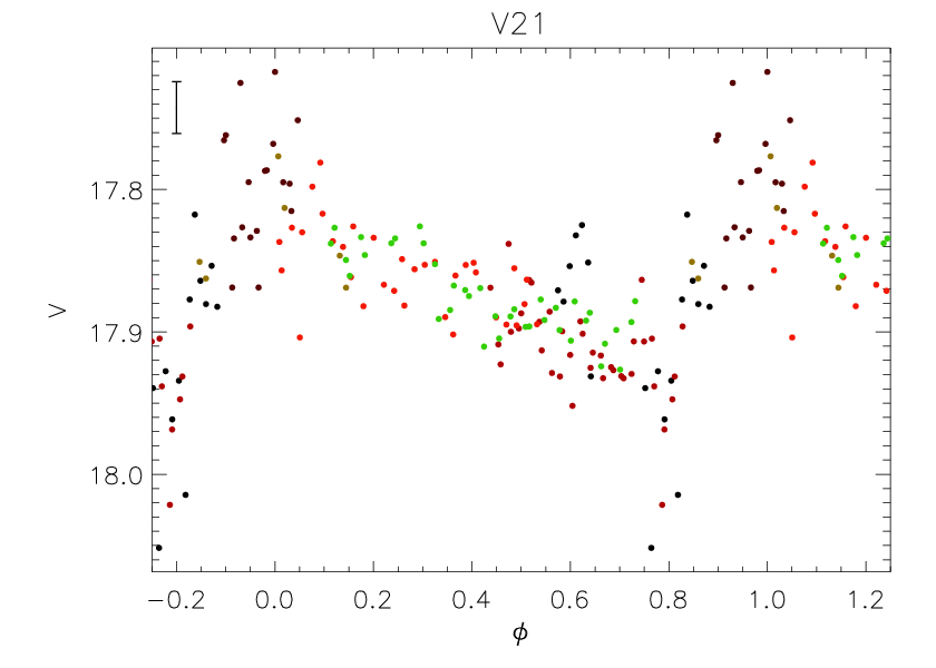
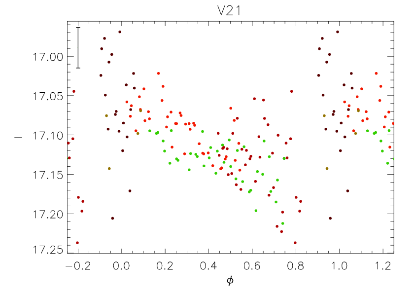
All confirmed variables are listed in Table 5, in which we also give epochs, periods and amplitudes. The corresponding light curves are showin in Figs. 4 and 5. A finding chart of the cluster with the location of the confirmed variables is shown in Fig. 6, and a CMD showing the locations of all confirmed variables is shown in Fig. 7.
| # | Epoch | (Rosino | (Pietrukowicz | Type | |||||
|---|---|---|---|---|---|---|---|---|---|
| (HJD-2450000) | (d) | 1949) (d) | et al. 2004) (d) | (mag) | (mag) | (mag) | (mag) | ||
| V1 | 6160.8234 | 0.7436296 | 0.74365a | 0.751 | 15.12 | 14.52 | 0.93 | 0.74 | RR0 |
| V2 | 6150.8616 | 0.6535119 | 0.6535049 | 15.20 | 14.62 | 0.92 | 0.65 | RR0 | |
| V3 | 6147.8307 | 0.6963265 | 0.69632 | 15.12 | 14.54 | 0.94 | 0.67 | RR0 | |
| V4b | 6147.8569 | 0.092318 | 20.19 | 19.14 | 2.74 | 1.91 | U Gem | ||
| V14 | 6150.8758 | 0.347953 | 15.18 | 14.77 | 0.48 | 0.32 | RR1 | ||
| V15 | 6160.7960 | 0.679015 | 0.689 | 15.07 | 14.52 | 1.08 | 0.68 | RR0 | |
| V16 | 6190.7559 | 0.325366 | 15.22 | 14.81 | 0.33 | 0.27 | RR1 | ||
| V17 | 6150.8805 | 0.059954 | 14.14 | 13.08 | 0.07 | 0.04 | SX Phoenicis + blend? | ||
| V18 | 6161.8536 | 0.307099 | 17.43 | 17.19 | 0.41 | 0.49 | Eclipsing blue straggler | ||
| V19c | 5779.8451 | 0.343379 | 0.341 | 13.85 | 13.10 | 0.15 | 0.11 | RR1 | |
| V20 | 6147.8377 | 0.040199 | 17.79 | 17.57 | 0.15 | 0.13 | SX Phoenicis | ||
| V21 | 6147.8589 | 0.113151 | 17.87 | 17.11 | 0.2 | ? |









3.4 Discussion of individual variables
We are unable to determine the nature of V17 with certainty. The combination of its position on the red giant branch and a short period of d makes it difficult to classify, although the shape of the light curve and the period would both be consistent with an SX Phoenicis variable blended with a red giant star (Darragh & Murphy 2012, e.g.). This is difficult to quantify, and higher-resolution data would be needed to investigate that possibility. From the position of V18 on the CMD and its light curve showing minima of different depths, we suggest that it is an eclipsing blue straggler binary system, of which only 6 examples are known in globular clusters (Kai & Sheng-Bang 2012). We classify V20 as an SX Phoenicis variable, from its light curve, period, and position on the CMD; we only identify one pulsation period for this variable. We could not reach any conclusion as to the nature of V21, because of the quality of its light curve; however variability is clear from both the and -band light curves, when discarding the poor-quality 2011 data, and data with large error bars, from the light curve. However we do verify that the variability of V21 is genuine in the difference images, and it is isolated, so there is no reason to believe that the variability is due to contamination from other variables. Below we discuss some of the variables in more detail.
3.4.1 V2
Figs. 4 and 5 show that our best period for V2 leads to an unsatisfactory phased light curve in both and . We suggest that the disjointed light curve may be due to a Blazhko effect (Blažko 1907) in this object; more observations are needed to confirm this.
3.4.2 V3
Like V2, but to a lesser extent, the light curves V3 seem disjointed, which we suggest may be due to a Blazhko effect. However, and more observations are needed to investigate this further.
3.4.3 V4
For the U Geminorum variable V4, we measured a quiet -band median magnitude of mag, while during outburst, we find a median magnitude of mag, giving an amplitude of 2.74 mag; in the band we find median values of (quiet) and (outburst), and an amplitude of 1.91 mag. Machin et al. (1991) found V4 to be significantly brighter, with mag, and Pietrukowicz et al. (2008) also found mag. It is interesting to note that, while our data only covers one outburst, the data covers three outburst, which show large variations in magnitude, by as much as mag between different outbursts.
We also conducted a period search for the quiet part of the light curve; Machin et al. (1991) used the quiescent colour they find from their spectra of this object, and the relations of Echevarria & Jones (1984) between and for dwarf novae, to conclude that the orbital period of V4 must be hours. We find a period during quiescence of days, or hours, in agreement with that conclusion. In Fig. 8, we show the phased quiescent light curves with this period, while the unphased light curve is shown in Fig. 9.


3.4.4 V16
The light curves in both and suggest that our single best period does not lead to a satisfactory phased light curve; we discuss possible explanations for this here. First we considered the possibility that V16 might be a double-mode RR Lyrae (RR01) star, which have only been detected in a few Galactic globular clusters (e.g. Nemec 1985; Clement et al. 1993; Clementini et al. 2004, and references therein). To investigate this, a search for the fundamental and first-overtone pulsation periods was conducted using the string-length method. We start by conducting a period search to identify a first period; for this we find . Assuming this to be the first-overtone period, and assuming an overtone-to-fundamental period ratio similar to what was found for double-mode RR Lyrae stars in M15, (Cox et al. 1983), we expect a fundamental period around . We pre-whiten our data for the first-overtone period to check whether we can recover this period. In the data, we find no evidence for such a period or any other pulsation period in our resulting power spectrum. We find similar results using the data, leading us to conclude that the unsatisfactory phasing of the V16 light curves is not due to double-mode pulsation.
Secondly, we also tried to fit the light curve by including a secular period change. To do this, we minimise the string length, but with a time-dependent period and phase ,
| (2) | |||||
| (3) |
where is the rate of change of the period and is the period at epoch . We varied within a small range near the value we found using the string-length method, and for each value of we explored a grid of values for ranging between and . From this we found that no such secular period change can explain the scatter in our phased light curve of V16.
This leads us to conclude that V16 either exhibits the Blazhko effect, or shows signs of non-radial pulsation. Amplitude variations are clear when comparing the 2011 (black filled circles on Fig. 4 and 5) and 2012 data, and Blazhko-like effects cause period modulations as well, which would explain that the light curve is not phased properly when using a single best-fit period. On the other hand, the scatter in the light curves, particularly in the band, is very similar to that observed in light curves of some of the variables in M 55 detected by Olech et al. (1999). They concluded that the scatter in the variations were caused by non-radial oscillations, and we suggest here that non-radial pulsation could also be the source of the scatter in the light curves of V16.
4 Fourier decomposition of RR Lyrae star light curves
Applying Fourier decomposition to the band light curves of RR Lyrae variables with sufficient phase coverage allows us to derive several of their properties, which we then use as a proxy for the parameters of their host cluster. Fourier decomposition consists in fitting light curves with the Fourier series
| (4) |
where is the magnitude at time , is the number of harmonics used in the fit, is the period of the variable, is the epoch, and and are the amplitude and phase of the harmonic. The Fourier parameters, which are epoch-independent, are then defined as
| (5) | |||||
| (6) |
In order to avoid over-fitting light curve features, we used the minimum number of harmonics that provided a good fit. Furthermore, for each variable, we checked the dependence on of the parameters we derive in the next sections. We found very little variation with , with any changes smaller than the error bars associated with the relevant quantities. In the following analysis, we excluded V16 because we suspect from its light curve that it may be affected by Blazhko effects or by non-radial pulsation (see Sec. 3.4).
We list the coefficients we obtained for the first four harmonics in Table 6, as well as the Fourier parameters and for the variables for which we could obtain a Fourier decomposition. We also list the deviation parameter , defined by Jurcsik & Kovács (1996) in order to assess whether fit parameters are reliable to derive properties of the RR Lyrae variables. Although Jurcsik & Kovács (1996) used a criterion whereby fits should have for their empirical relations to yield reliable estimates of stellar properties, a less stringent criterion of has been used by other authors (Cacciari et al. 2005, e.g.). Here we also adopt as a selection criterion to estimate stellar properties.
Although some acceptable fits could be obtained for V2, with , we exclude it from the analysis as well because we suspect its light curve might be affected by Blazhko effects. Furthermore, the value of the physical parameters is very sensitive to the number of harmonics used in the fit. Although we suggested in Sec. 3.4 that V3 might also be affected by Blazhko effects, we find that the Fourier fits and resulting physical parameters are stable for V3, and therefore include it in the following analysis. We note, however, that this may account for the larger value of we find for V3. We also exclude V19 because our phase coverage does not enable us to find a good Fourier fit. This leaves us with 4 RR Lyrae stars with good Fourier decompositions, three RR0 (V1, V3 and V15) and one RR1 (V14).
| # | ||||||||||
|---|---|---|---|---|---|---|---|---|---|---|
| RR0 | ||||||||||
| V1 | 15.121(2) | 0.337(2) | 0.160(2) | 0.110(2) | 0.050(2) | 4.045(12) | 8.498(16) | 6.581(22) | 7 | 2.6 |
| V2a | 15.196(2) | 0.320(2) | 0.134(2) | 0.107(2) | 0.081(2) | 4.005(11) | 8.511(15) | 6.668(16) | 7 | 3.0 |
| V3 | 15.118(2) | 0.319(2) | 0.152(2) | 0.112(2) | 0.059(2) | 3.973(11) | 8.413(13) | 6.468(19) | 7 | 4.9 |
| V15 | 15.067(2) | 0.344(2) | 0.181(2) | 0.122(1) | 0.081(2) | 3.987(7) | 8.274(12) | 6.431(14) | 10 | 2.5 |
| RR1 | ||||||||||
| V14 | 15.176(2) | 0.214(3) | 0.030(3) | 0.012(2) | 0.010(2) | 4.773(26) | 2.673(137) | 2.338(104) | 6 |
4.1 Metallicity
We use the empirical relations of Jurcsik & Kovács (1996) to derive the metallicity [Fe/H] for each of the variables for which we could obtain a successful Fourier decomposition. The relation is derived from the spectroscopic metallicity measurement of field RR0 variables, and it relates [Fe/H] to the period and the Fourier parameter , where denotes a parameter obtained by fitting a sine series rather than the cosine series we fit with Eq. (4). [Fe/H] is then expressed as
| (7) |
where the subscript J denotes a non-calibrated metallicity, the period P is in days, and can be calculated via
| (8) |
We transform these to the metallicity scale of Zinn & West (1984) (hereafter ZW) using the relation from Jurcsik (1995):
| (9) |
However Kovács (2002) noted that for metal-poor clusters, Eq. (7) yields metallicity values that are too large by dex. This was also confirmed by Gratton et al. (2004) and Di Fabrizio et al. (2005) by comparing spectroscopic and Fourier-decomposition metallicity values for RR Lyrae in the Large Magellanic Cloud (LMC). Therefore here we include a shift of -0.20 dex (on the scale) to metallicity values we derive for RR0 stars using Eq. (7), which corresponds to a shift on the ZW scale of -0.14 dex.
For the RR1 variables, we calculated the metallicity using the empirical relation of Morgan et al. (2007), linking [Fe/H], and :
| (10) | |||||
| # | ||||
|---|---|---|---|---|
| RR0 | ||||
| V1 | -2.04(2) | 0.351(2) | 1.780(1) | 6187(7) |
| V3 | -1.95(2) | 0.428(2) | 1.746(1) | 6247(6) |
| V15 | -2.01(2) | 0.428(2) | 1.746(1) | 6249(5) |
| RR1 | ||||
| V14 | -2.03(4) | 0.540(6) | 1.650(3) | 7180(13) |
4.2 Effective Temperature
The Fourier parameters can also be used to calculate the effective temperature, using empirical relations derived by Jurcsik (1998). Those relations link the colour to as well as several of the Fourier coefficients and parameters:
| (11) | |||||
| (12) | |||||
For RR1 variables, Simon & Clement (1993) used theoretical models to derive an empirical relation,
| (13) |
We list the temperatures we derived for each RR Lyrae star in Table 7. As noted in our previous analyses, there are several caveats to deriving temperatures with Eq. (12) and (13). These relations yield values of for RR0 and RR1 stars on different absolute scales. Furthermore, the effective temperatures we derive here show systematic deviations from the relations predicted by evolutionary models of Castelli (1999) or the temperature scales of Sekiguchi & Fukugita (2000). Bearing these caveats in mind, we use these relations to derive temperature estimates in order to be consistent with our previous studies.
4.3 Absolute Magnitude
Kovács & Walker (2001) derived empirical relations to calculate V-band absolute magnitudes for the RR0 variables, linking the magnitude to Fourier coefficients through
| (14) |
where is a constant. As in our previous studies, we adopt a value of mag to be consistent with a true LMC distance modulus of mag (Freedman et al. 2001). For RR1 variables, we use the relation of Kovács (1998),
| (15) |
where is a constant, for which we choose a value of 1.061 with the same justification as for our choice of .
We also converted the magnitudes we obtained to luminosities using
| (16) |
where is the bolometric magnitude of the Sun, , and is a bolometric correction which we determine by interpolating from the values of Montegriffo et al. (1998) for metal-poor stars, and using the value of we derived in the previous section. Values of and for the RR0 and RR1 variables are listed in Table 7. Using our average values of , in conjunction with the average values of (Sec. 4.1), we find a good agreement with the relation derived in the literature (e.g. Kains et al. 2012, see Fig.9 of that paper).
5 Cluster properties
5.1 Oosterhoff Type
We find mean periods d and d, with a proportion of 43% of the RR Lyrae in this cluster being of RR1 type.
From these values of and the fraction of RR1 stars in M 30, as well as its low metallicity, we confirm previous classification of this cluster in the literature as Oosterhoff type II (Lee & Carney 1999, e.g.). This is also confirmed by comparing the locations of our variables on a Bailey diagram (Fig. 10) to the tracks derived by Cacciari et al. (2005) for evolved stars.


5.2 Distance
5.2.1 Using the RR Lyrae stars
We can use the parameter from our Fourier decompositions, which corresponds to the mean apparent V magnitude of the RR Lyrae, as well as the absolute magnitudes of the RR Lyrae we derived in Sec. 4.3 to derive the distance modulus to M 30. The mean value of the for our RR0 variables is 15.09 0.03 mag, while the mean of the absolute magnitudes is 0.40 0.04 mag. This yields a distance modulus of mag. Using the parameters for our RR1 variable (V14, see Tables 6 & 7), we find mag.
The reddening towards this cluster has been estimated in the literature by several authors, with values of ranging from 0.01 to 0.12 mag. Zinn (1980) derived a value of mag from integrated light measurements, Bolte (1987) adopted a value of mag, while Richer et al. (1988) found a value of mag; Piotto et al. (1990) derived mag from their CMD analysis, and Samus et al. (1995) found values of or 0.12 mag, depending on the metallicity of the isochrone they fitted to their CMD. Ferraro et al. (1999) report a value for this cluster mag.
Here we adopt a value of mag, as well as a value of for our Galaxy. We use these to derive mean true distance moduli of mag and mag, from our RR0 and RR1 variables respectively. These values correspond to mean physical distances of kpc and 8.10 kpc. Since the distance values are sensitive to our chosen value of , we also derive distances using the largest value of reddening in the literature mag, to find a lower limit for the distances of and 7.13 kpc. Our values for the distance to the cluster are consistent with previous estimates in the literature, reported in Table 8.
5.2.2 Using SX Phoenicis stars
SX Phoenicis stars can be used as standard candles thanks to their period-luminosity () relation (Jeon et al. 2003, e.g.), allowing us to estimate the distance to M 30 using the detected SX Phoenicis star in our sample, V20. We use the relation of Cohen & Sarajedini (2012),
| (17) |
where denotes the fundamental-mode pulsation period. Using d for V20, we find mag. Using a mean magnitude of mag, mag, this yields a distance modulus of mag, which corresponds to a physical distance of kpc, in excellent agreement with the distance calculated using the RR Lyrae stars, and consistent with estimates in the literature.
| Reference | [mag] | Distance [kpc] | Method |
|---|---|---|---|
| This work | 14.60 0.05 | 8.32 0.20 | Fourier decomposition of RR0 light curves |
| This work | 14.54 | 8.10 | Fourier decomposition of RR1 light curves |
| This work | 14.61 0.11 | 8.35 0.42 | SX Phoenicis relation |
| Carretta et al. (2000) | 14.88 0.05 | 9.46 0.22 | Parallax of local subdwarfs |
| Ferraro et al. (1999) | 14.71 | 8.75 | Magnitude of the horizontal branch |
| Sandquist et al. (1999) | 14.65 0.12 | 8.51 0.47 | Parallax of local subdwarfs |
| Sandquist et al. (1999) | 14.87 0.12 | 9.42 0.52 | Parallax of local subdwarfs |
| Gratton et al. (1997) | 14.94 0.08 | 9.72 0.36 | Parallax of local subdwarfs |
| Bergbusch (1996) | 14.83 | 9.25 | CMD analysis |
| Samus et al. (1995) | 14.70 0.10 | 8.71 0.40 | CMD analysis |
| Piotto et al. (1990) | 14.65 0.15 | 8.51 0.59 | CMD analysis |
| Piotto et al. (1987) | 14.50 0.50 | 7.94 1.83 | CMD analysis |
| Bolte (1987) | 14.65 | 8.51 | Parallax of local subdwarfs |
5.3 Metallicity
Although the relation of Sandage (2006) relating the mean period of RR0 stars to the cluster metallicity is not applicable for Oosterhoff type II clusters (Clement et al. 2001), we can use the metallicities we calculated in Sec. 4.1 for the RR Lyrae stars in the cluster to derive an estimate for the metallicity of M 30. To do this, we simply compute an average of the RR Lyrae metallicities given in Table 7, excluding the variables for which the metallicity estimate is unreliable. Assuming that there is no systematic offset between the different types of variables, as in previous studies (Kains et al. 2012; Bramich et al. 2011), we find a mean metallicity , in good agreement with values found in the literature (see Table 9).
Carretta et al. (2009a) derived a new metallicity scale based on GIRAFFE and UVES spectra of red giant branch (RGB) stars in 19 globular clusters, which is now widely used to quote metallicity values for globular clusters. The transformation from the ZW to the UVES (Carretta et al. 2009a) scale is given as
| (18) |
Using this we find a metallicity for M 30 of , significantly higher than the value found for this cluster by Carretta et al. (2009b) of .
| Reference | Method | ||
|---|---|---|---|
| This work | -2.01 0.04 | Fourier decomposition of RR Lyrae light curves | |
| Carretta et al. (2009b) | -2.04 0.16 | UVES spectroscopy of red giants | |
| Carretta et al. (2009c) | -2.05 0.16 | FLAMES/GIRAFFE specta of red giants | |
| Sandquist et al. (1999) | -2.01 0.09 | Simultaneous reddening-metallicity method | |
| Bergbusch (1996) | -2.03 | -2.14 | CMD isochrone fitting |
| Minniti et al. (1993) | -2.11 0.08 | Spectroscopy of red giants | |
| Claria et al. (1988) | -2.4 | Spectroscopy of red giants | |
| Bolte (1987) | -2.03 0.13 | CMD isochrone fitting | |
| Smith (1984) | -2.02 0.14 | spectral index | |
| Zinn & West (1984) | -2.13 0.13 | spectral index | |
| Zinn (1980) | -1.96 0.12 | spectral index |
5.4 Age
We use our CMD to derive an estimate for the age of M 30, by fitting to it the isochrones of VandenBerg & Clem (2003), using our estimate of the cluster metallicity, . We also used a value for the enhancement of (Dotter et al. 2010). From the best-fitting isochrones, we estimate the age of the cluster to be Gyr, in good agreement with recent estimates in the literature (see Table 10). A set of isochrones is overplotted on the CMD in Fig. 7.
| Reference | Age [Gyr] | Method |
|---|---|---|
| This work | 13 1 | CMD isochrone fitting |
| Dotter et al. (2010) | 13.25 1.00 | CMD isochrone fitting |
| Carretta et al. (2000) | 12.3 | Parallax of local subdwarfs |
| Bergbusch (1996) | 14 | CMD isochrone fitting |
| Samus et al. (1995) | 17 | CMD isochrone fitting |
| Samus et al. (1995) | 15 | CMD isochrone fitting |
| Piotto et al. (1990) | 16 2 | CMD isochrone fitting |
| Bolte (1987) | 17 | CMD isochrone fitting |
6 Conclusions
We have used and band observations spanning a baseline of months to survey stellar photometric variability in M 30. This allows us to update the catalogue of variables in this cluster significantly, with detections and refined analysis of three previously known RR Lyrae stars, one known U Gem star, as well as of two candidate RR Lyrae stars, to which we assigned catalogue numbers. Furthermore, we detect previously unknown variables, including two RR1 stars, an SX Phoenicis star, an eclipsing blue straggler system, and two variables that we are unable to classify with certainty. We provide refined period estimates for all variables, and then carry out Fourier decomposition of RR Lyrae stars. Using the Fourier parameters of stars for which this was successful, we derive properties for the RR Lyrae, and use these as proxies for the cluster’s properties.
We find a cluster metallicity of , or , and distances of or 8.10 kpc, using RR0 and RR1 stars respectively. Our light curve of the SX Phoenicis variable V20 also affords another way to estimate the cluster distance; using this, we find a distance of kpc. Our CMD also allows us to estimate the age of the cluster by fitting isochrones to it. We find an age of Gyr. All of these values are in good agreement with estimates in the literature, and are independent estimates calculated for the first time using Fourier decomposition of RR Lyrae in this cluster.
Acknowledgements
We thank the referee Christine Clement for constructive comments. NK acknowledges an ESO Fellowship. The research leading to these results has received funding from the European Community’s Seventh Framework Programme (/FP7/2007-2013/) under grant agreement No 229517. AAF acknowledges the support of DGAPA-UNAM through project IN104612. AAF and SG are thankful to the CONACyT (México) and the Department of Science and Technology (India) for financial support under the Indo-Mexican collaborative project DST/INT/MEXICO/RP001/2008. OW (aspirant FRS - FNRS), AE (post-doc PRODEX), YD (post-doc PRODEX) and J. Surdej acknowledge support from the Communauté française de Belgique – Actions de recherche concertées – Académie universitaire Wallonie-Europe. TCH gratefully acknowledges financial support from the Korea Research Council for Fundamental Science and Technology (KRCF) through the Young Research Scientist Fellowship Program. TCH acknowledges financial support from KASI (Korea Astronomy and Space Science Institute) grant number 2012-1-410-02. KA, DB, MD, MH, and CL are supported by NPRP grant NPRP-09-476-1-78 from the Qatar National Research Fund (a member of Qatar Foundation). The Danish 1.54m telescope is operated based on a grant from the Danish Natural Science Foundation (FNU). Funding for the Stellar Astrophysics Centre at Aarhus University is provided by The Danish National Research Foundation. This research was supported in part by the ASTERISK project (ASTERoseismic Investigations with SONG and Kepler), funded by the European Research Council (Grant agreement no.: 267864). CS received funding from the European Union Seventh Framework Programme (FP7/2007-2013) under grant agreement no. 268421. CHG and XSF acknowledge support from National Natural Science Foundation of China (grants Nos. 10373023 and 10773027). HK acknowledges support from a Marie-Curie Intra-European Fellowship.
References
- Allen et al. (2006) Allen, C., Moreno, E., & Pichardo, B. 2006, ApJ, 652, 1150
- Arellano Ferro et al. (2013) Arellano Ferro, A., Bramich, D. M., Figuera Jaimes, R., et al. 2013, in prep.
- Arellano Ferro et al. (2011) Arellano Ferro, A., Figuera Jaimes, R., Giridhar, S., et al. 2011, MNRAS, 416, 2265
- Bailey (1902) Bailey, S. I. 1902, Annals of Harvard College Observatory, 38, 1
- Bergbusch (1996) Bergbusch, P. A. 1996, AJ, 112, 1061
- Blažko (1907) Blažko, S. 1907, Astronomische Nachrichten, 175, 325
- Bolte (1987) Bolte, M. 1987, ApJ, 319, 760
- Bramich (2008) Bramich, D. M. 2008, MNRAS, 386, L77
- Bramich et al. (2011) Bramich, D. M., Figuera Jaimes, R., Giridhar, S., & Arellano Ferro, A. 2011, MNRAS, 413, 1275
- Bramich & Freudling (2012) Bramich, D. M. & Freudling, W. 2012, MNRAS, 424, 1584
- Bramich et al. (2013) Bramich, D. M., Horne, K., Albrow, M. D., et al. 2013, MNRAS, 428, 2275
- Cacciari et al. (2005) Cacciari, C., Corwin, T. M., & Carney, B. W. 2005, AJ, 129, 267
- Carretta et al. (2009a) Carretta, E., Bragaglia, A., Gratton, R., D’Orazi, V., & Lucatello, S. 2009a, A&A, 508, 695
- Carretta et al. (2009b) Carretta, E., Bragaglia, A., Gratton, R., & Lucatello, S. 2009b, A&A, 505, 139
- Carretta et al. (2009c) Carretta, E., Bragaglia, A., Gratton, R. G., et al. 2009c, A&A, 505, 117
- Carretta et al. (2000) Carretta, E., Gratton, R. G., Clementini, G., & Fusi Pecci, F. 2000, ApJ, 533, 215
- Castelli (1999) Castelli, F. 1999, A&A, 346, 564
- Claria et al. (1988) Claria, J. J., Minniti, D., & Gomez, M. N. 1988, A&A, 199, L1
- Clement et al. (1993) Clement, C. M., Ferance, S., & Simon, N. R. 1993, ApJ, 412, 183
- Clement et al. (2001) Clement, C. M., Muzzin, A., Dufton, Q., et al. 2001, AJ, 122, 2587
- Clementini et al. (2004) Clementini, G., Corwin, T. M., Carney, B. W., & Sumerel, A. N. 2004, AJ, 127, 938
- Cohen & Sarajedini (2012) Cohen, R. E. & Sarajedini, A. 2012, MNRAS, 419, 342
- Cox et al. (1983) Cox, A. N., Hodson, S. W., & Clancy, S. P. 1983, ApJ, 266, 94
- Darragh & Murphy (2012) Darragh, A. N. & Murphy, B. W. 2012, Journal of the Southeastern Association for Research in Astronomy, 6, 72
- Di Fabrizio et al. (2005) Di Fabrizio, L., Clementini, G., Maio, M., et al. 2005, A&A, 430, 603
- Djorgovski & King (1986) Djorgovski, S. & King, I. R. 1986, ApJ, 305, L61
- Dotter et al. (2010) Dotter, A., Sarajedini, A., Anderson, J., et al. 2010, ApJ, 708, 698
- Echevarria & Jones (1984) Echevarria, J. & Jones, D. H. P. 1984, MNRAS, 206, 919
- Ferraro et al. (1999) Ferraro, F. R., Messineo, M., Fusi Pecci, F., et al. 1999, AJ, 118, 1738
- Forbes & Bridges (2010) Forbes, D. A. & Bridges, T. 2010, MNRAS, 404, 1203
- Freedman et al. (2001) Freedman, W. L., Madore, B. F., Gibson, B. K., et al. 2001, ApJ, 553, 47
- Gratton et al. (2004) Gratton, R. G., Bragaglia, A., Clementini, G., et al. 2004, A&A, 421, 937
- Gratton et al. (1997) Gratton, R. G., Fusi Pecci, F., Carretta, E., et al. 1997, ApJ, 491, 749
- Jeon et al. (2003) Jeon, Y.-B., Lee, M. G., Kim, S.-L., & Lee, H. 2003, AJ, 125, 3165
- Jurcsik (1995) Jurcsik, J. 1995, Act. Astron., 45, 653
- Jurcsik (1998) Jurcsik, J. 1998, A&A, 333, 571
- Jurcsik & Kovács (1996) Jurcsik, J. & Kovács, G. 1996, A&A, 312, 111
- Kai & Sheng-Bang (2012) Kai, L. & Sheng-Bang, Q. 2012, AJ, 144, 161
- Kains et al. (2012) Kains, N., Bramich, D. M., Figuera Jaimes, R., et al. 2012, A&A, 548, A92
- Kovács (1998) Kovács, G. 1998, Mem. Soc. Astron. Ital., 69, 49
- Kovács (2002) Kovács, G. 2002, in Astronomical Society of the Pacific Conference Series, Vol. 265, Omega Centauri, A Unique Window into Astrophysics, ed. F. van Leeuwen, J. D. Hughes, & G. Piotto, 163
- Kovács & Walker (2001) Kovács, G. & Walker, A. R. 2001, A&A, 371, 579
- Lafler & Kinman (1965) Lafler, J. & Kinman, T. D. 1965, ApJS, 11, 216
- Lee & Carney (1999) Lee, J.-W. & Carney, B. W. 1999, AJ, 118, 1373
- Machin et al. (1991) Machin, G., Callanan, P. J., Allington-Smith, J., Charles, P. A., & Hassall, B. J. M. 1991, MNRAS, 250, 602
- Margon & Downes (1983) Margon, B. & Downes, R. A. 1983, ApJ, 274, L31
- Minniti et al. (1993) Minniti, D., Geisler, D., Peterson, R. C., & Claria, J. J. 1993, ApJ, 413, 548
- Monet et al. (2003) Monet, D. G., Levine, S. E., Canzian, B., et al. 2003, AJ, 125, 984
- Montegriffo et al. (1998) Montegriffo, P., Ferraro, F. R., Origlia, L., & Fusi Pecci, F. 1998, MNRAS, 297, 872
- Morgan et al. (2007) Morgan, S. M., Wahl, J. N., & Wieckhorst, R. M. 2007, MNRAS, 374, 1421
- Nemec (1985) Nemec, J. M. 1985, AJ, 90, 240
- Olech et al. (1999) Olech, A., Kaluzny, J., Thompson, I. B., et al. 1999, AJ, 118, 442
- Padmanabhan et al. (2008) Padmanabhan, N., Schlegel, D. J., Finkbeiner, D. P., et al. 2008, ApJ, 674, 1217
- Pietrukowicz & Kaluzny (2004) Pietrukowicz, P. & Kaluzny, J. 2004, Act. Astron., 54, 19
- Pietrukowicz et al. (2008) Pietrukowicz, P., Kaluzny, J., Schwarzenberg-Czerny, A., et al. 2008, MNRAS, 388, 1111
- Piotto et al. (1987) Piotto, G., Capaccioli, M., Ortolani, S., et al. 1987, AJ, 94, 360
- Piotto et al. (1990) Piotto, G., King, I. R., Capaccioli, M., Ortolani, S., & Djorgovski, S. 1990, ApJ, 350, 662
- Richer et al. (1988) Richer, H. B., Fahlman, G. G., & Vandenberg, D. A. 1988, ApJ, 329, 187
- Rosino (1949) Rosino, L. 1949, Mem. Soc. Astron. Ital., 20, 63
- Rosino (1961) Rosino, L. 1961, Asiago-Padova Cont., 117
- Samus et al. (1995) Samus, N. N., Ipatov, A. P., Smirnov, O. M., et al. 1995, Astronomy Letters, 21, 810
- Sandage (2006) Sandage, A. 2006, AJ, 131, 1750
- Sandquist et al. (1999) Sandquist, E. L., Bolte, M., Langer, G. E., Hesser, J. E., & Mendes de Oliveira, C. 1999, ApJ, 518, 262
- Sekiguchi & Fukugita (2000) Sekiguchi, M. & Fukugita, M. 2000, AJ, 120, 1072
- Simon & Clement (1993) Simon, N. R. & Clement, C. M. 1993, ApJ, 410, 526
- Skottfelt et al. (2013) Skottfelt, J., Bramich, D. M., Figuera Jaimes, R., et al. 2013, ArXiv e-prints
- Smith (1984) Smith, H. A. 1984, ApJ, 281, 148
- Smitka & Layden (2010) Smitka, M. T. & Layden, A. C. 2010, in Bulletin of the American Astronomical Society, Vol. 36, American Astronomical Society Meeting Abstracts 215, 606.18
- Stellingwerf (1978) Stellingwerf, R. F. 1978, ApJ, 224, 953
- Stetson (2000) Stetson, P. B. 2000, PASP, 112, 925
- Terzan (1968) Terzan, A. 1968, Publications of the Observatoire Haute-Provence, 9, 24
- Terzan & Rutily (1975) Terzan, A. & Rutily, B. 1975, A&A, 38, 307
- VandenBerg & Clem (2003) VandenBerg, D. A. & Clem, J. L. 2003, AJ, 126, 778
- Zinn (1980) Zinn, R. 1980, ApJS, 42, 19
- Zinn & West (1984) Zinn, R. & West, M. J. 1984, ApJS, 55, 45