Monte Carlo approximation to optimal investmentThanks: Statistical Laboratory, Wilberforce Road, Cambridge CB3 0WB, United Kingdom.
Abstract
This paper sets up a methodology for approximately solving optimal investment problems using duality methods combined with Monte Carlo simulations. In particular, we show how to tackle high dimensional problems in incomplete markets, where traditional methods fail due to the curse of dimensionality.
1 Introduction.
From the early work of Merton and his seminal papers [6] and [5], the optimal investment literature has been trying to determine how to invest in financial markets when facing uncertainty. Over the following twenty years, many general results were proved, and many techniques for tackling the questions developed.
Deriving the abstract forms of the solutions is a great achievement of mathematical finance. However, anyone who wants to use them to guide them in making investment decisions will quickly find out that they are typically rather uninformative. This is because, apart from a couple of highly stylized examples, concrete numerical answers in optimal investment problems are simply unobtainable, largely due to the curse of dimensionality. See [9] for a survey of the traditional methods and a range of examples where answers can actually be found.
The goal of this paper is to take a pragmatic approach. We take the point of view of an investor who is facing a particular market and is interested in knowing a good thing to do at a particular time. Hence, we want to be able to describe what a good investment strategy is in a particular market environment without computing the whole value function for the problem, and we want to quantify what we mean by a good investment strategy, in terms of bounds on the objective.
Taking this standpoint lets us make progress by combining various optimization techniques that would fail individually when applied to difficult optimal investment problems. Namely, we shall use the Pontryagin–Lagrange approach to determine locally optimal trajectories; the dual formulation of the optimal investment problem to derive bounds on the optimal trajectory; and Monte Carlo techniques to approximate the expectation operator.
Combining these related methods lets us handle a surprisingly large class of problems. We will show how to find approximately optimal investment paths for any continuous-path incomplete market driven by a diffusion factor process. As an illustration of the effectiveness of the method, we shall provide a couple of numerical examples. We shall start with the benchmark Merton problem, moving on to problems that are increasingly more difficult to handle numerically and mathematically.
This paper is structured as follows. In Section 2 we present the general problem and the methodology for solving it. Section 3 describes the algorithms used in the method. In Section 4 we give numerical evidence for the performance of the method, considering examples of the Merton problem, the non-constant relative risk aversion, and finally a multi-dimensional incomplete market driven by a diffusion. Section 5 concludes.
2 Continuous markets driven by a diffusion.
We shall present the methodology in the context of a finite-horizon optimal investment-consumption problem where the volatilities and drifts of the assets depend on some diffusion factor process. It will become evident that the general approach is not limited to such examples, but it is easier to explain in this more concrete setting. We shall also make various assumptions of boundedness on processes and global Lipschitz properties of coefficients which could be relaxed, but which simplify the exposition and proof: the aim is transparency, not maximality.
To begin with, suppose that is an -valued diffusion process satisfying
| (2.1) |
where is a -dimensional Brownian motion, and and are globally Lipschitz coefficients.
We shall consider an investor who is allowed to invest in a market with a riskless asset yielding interest at rate , and stocks having volatility matrix and drift . Here, , , and are bounded measurable functions. We assume non-degeneracy of the market, that is, , and that the row rank of equals . When , the matrix is then invertible, and we have a special case of a complete market.
With these assumptions in place, the investor’s wealth at time evolves11 1 We use the notations for the scalar product of two vectors and , and for the column vector of ones. as
| (2.2) |
where the -vector process represents the cash holdings in each of the stocks, and denotes the agent’s consumption rate. The agent’s objective at time is to achieve
| (2.3) |
where and are strictly concave utility functions satisfying the Inada conditions22 2 These are the conditions , . , and denotes the set of admissible consumption-portfolio pairs:
| (2.4) |
Remarks. (i) Notice that the function is defined on the whole of .
(ii) The above definition of admissibility (2.4) is not the usual one33 3 One typically imposes a non-negativity constraint on the wealth process associated with the trading strategy .. We do not expect that the supremum in (2.3) will be attained within the set , but as our goal is to come up with good sub-optimal strategies, this does not matter for our current purposes. Admissibility is imposed to eliminate doubling strategies, where wealth may go arbitrarily negative before time , but ends up at a high value at time . The assumptions made here rule this out; if we were to go to large negative wealth at some time in , boundedness of , and prevent us returning to positive wealth with certainty by time , and the penalty imposed by the concave function then makes this a bad thing to do.
(iii) If the dimension of the statespace of the factor diffusion were not very small, it is not feasible to calculate and store the value function . The approach we develop in this paper allows us to determine approximately optimal policies without the need to calculate .
We shall require one technical condition on , which is expressed as a condition on the inverse marginal utility , defined by
| (2.5) |
We require
| (2.6) |
The inequality has to hold for all and all
We are now ready to state the main result of the paper, which allows us to derive effective Monte Carlo bounds on the value, and to find good sub-optimal strategies pathwise. The proof uses duality arguments similar to those presented in [2], [4], and later described in a more general setting in [3].
Theorem 2.1.
Suppose that is a bounded previsible process such that
| (2.7) |
and that solves the linear SDE
| (2.8) |
Define the function by44 4 The functions , are the convex dual functions, , .
| (2.9) |
for , , . Then for any , , , , and bounded previsible , we have the inequalities
| (2.10) |
where
| (2.11) |
and the process is the solution to the wealth evolution (2.2) with portfolio process and consumption process
| (2.12) |
Remarks. (i) In general the matrix is not even square, so not invertible, but we could try to find to satisfy (2.7) by taking the pseudo-inverse of :
| (2.13) |
This can be done if is bounded, in effect a uniform ellipticity condition of the kind commonly imposed in such problems.
(ii) From the definition of the convex dual function , it is clear that is always non-negative. Since dominates the gap between the lower and upper bounds, we should aim to make as small as we can. Ideally, we would have that was zero, which would require us to have
| (2.14) |
If we demanded that this happens, then the problem becomes a BSDE with (2.14) as the terminal condition. As it seems that there are as yet no efficient numerical methods for solving BSDEs in high dimensions, this does not help much. What we are attempting to do with this approach is in effect relax the demand that the solution we construct hits the terminal condition (2.14), but instead to estimate the error we make when we fail to match the terminal condition.
Proof. (a) The upper bound. The process is determined by (2.7) and (2.8); in what follows, we shall suppose that is determined from by (2.12).
We claim that the stochastic integral has zero mean, and in order to establish this, it is necessary to control the integrand. The processes , , and are all bounded by hypothesis, so we need to have control on and . Since satisfies the linear SDE (2.8) with bounded coefficients and , it is not hard to establish a bound on for any , and for any , where ; see, for example, Lemma V.11.5 of [10]. Similarly, we may bound for any , and for any , by considering the linear SDE for . All that remains is to establish a similar bound for , where is given by (2.2). The only problematic part of this estimation is in controlling , but this is where the Assumption (2.6) comes in, since is controlled as before, and is bounded by some power of .
We therefore conclude that
| (2.16) |
We can add this equality to (2.3) to find55 5 We use (2.12) at the first step.
| (2.17) | |||||
| (2.18) |
This is the upper bound in (2.10).
(B) The lower bound. The argument reuses elements of the proof of the upper bound. The task this time is to propose some admissible and deduce a lower bound from it.
Given the state-price density process as in (2.8), our intention is to use the process to be defined from it by (2.12). Doing this, we see that the integral term appearing in the right-hand side of (2.17) is equal to
and moreover that (2.16) still holds by the same argument as before. For any bounded previsible , the pair is admissible, so if we use that admissible pair we find as at (2.17) that
| (2.19) | |||||
Remarks. (i) For any bounded previsible and
the result (2.10) of Theorem 2.1 gives two-sided bounds
on the value function. Importantly, the numerical values of and
can be estimated by forward simulation from current values.
It is also worth noting that the methodology does not require any
‘simulation within simulations’ which substantially increases the
computation times; we will be evaluating the state-price density and
the portfolio process along just one trajectory.
All we need to do is to simulate
sufficiently many sample paths to approximate the
expectation operator in (2.9) and (2.11).
(ii) We need to have a measure for comparison
between the bounds in (2.10). Since utility
functionals are defined up to affine transformations, our
measure needs to be invariant under those. Thus
the difference between the upper and lower bounds is not
informative.
We can however think of giving up a fraction of the initial wealth and look for the minimal such that the upper bound corresponding to initial wealth is at most as large as the lower bound for starting with wealth . This is of course:
| (2.20) |
which will from now on be our efficiency measure. Notice that (2.20) is
a dimensionless quantity.
(iii) The key issue for obtaining good bounds is of course the
choice of the processes and .
The traditional way to approach solving the problem (2.3) would
be to write down the HJB equation, derive the corresponding PDEs,
and try to solve them. However, these PDEs are typically highly
non-linear, and we only stand a chance of getting reasonably
stable solutions in dimensions one or two.
Nevertheless, we can deduce some worthwhile information from the HJB equation. Dropping the subscript, and remembering the function takes as arguments, the HJB equation is
| (2.21) | |||||
Optimizing over leads to the conclusion that , and optimizing over tells us that we should have
| (2.22) |
Here is invertible by our non-degeneracy assumptions on the market.
Assuming that and are dual (as we would expect from (2.10)), in that
| (2.23) |
this would lead us to the relations
| (2.24) |
Straightforward calculus then leads to
| (2.25) |
These relations help us to make choices of and . We will use (2.13) to make our (pathwise) choice for , and then we will use the truncated form
| (2.26) |
for the pathwise choice of . We should in principle include the cross derivative term from (2.22) in the choice of , and in some situations it might well be worth doing this, but the cost is that we have to get hold of the derivative of with respect to , and doing this by simulation is cumbersome. The virtue of the form (2.26) is that we just need the second derivative of the convex function with respect to its scalar argument , and determining this by simulation is computationally feasible.
(iv) In practice, it will be clumsy to form an estimate of the term in (2.10) if we are determining the portfolio process according to the recipe just outlined, because if we are to simulate an evolution of we will at each step need to identify derivatives of , and this is a simulation within a simulation. We envisage the lower bound in (2.10) being used as a means to assess a particular portfolio rule which may be expressed explicitly as some function of . In a high-dimensional problem, we do not expect the optimal portfolio rule to be something we can characterize, but we may well have some heuristic for some ‘good’ portfolio rule, and (2.10) gives us a way to tell how good that heuristic may be.
Summarising: Given an initial state , we can follow the dynamics of , , and , using (2.1), (2.2), (2.8), given by (2.7), given by (2.12), and given by (2.26) (or perhaps (2.22)).
The key advantage of this formulation is that all we need to do now is to optimise the bounds (2.10) for a one-dimensional starting value of the dual process . This is a quick procedure numerically.
3 Algorithms.
We will now describe an algorithm for simulating the optimal path and controls for the problem (2.3), given a particular realisation of the Brownian motion. That is, we do not attempt to recover the whole value function, as this is bound to fail in higher dimensions. Our method, which is effectively local, will follow a particular realisation of the Brownian motion and tell us how to invest and consume in that particular case. After all, one is predominantly interested in how to invest in the current market conditions, and does not necessarily care about all possible versions of reality!
| Step 1: | Initialisation. Pick starting values , and a grid of time steps along which we want to know the solution. Simulate a realisation of the Brownian motion along which we want to calculate the optimal path. |
|---|---|
| Step 2: | Finding the optimal . For any , we can calculate . This function is convex in , so we can use the golden Section search to find the minimum in (2.23). This gives us the value of and the optimal starting value of the dual process . |
| Step 3: | Calculating the optimal path. For each , we have available. We use (2.12) to work out , (2.26) to work out , and (2.24) to work out . We then cacluate wth (2.7) and use the Euler scheme to move to time using (2.1) and (2.8). |
Algorithm 1 describes how to compute the best bounds numerically. The cost of running this algorithm will be , where is the average cost of evaluation of the function and .
In Algorithm 1, we have not yet given the details of how to calculate the function numerically (which will be the business of Algorithm 2). That is, we want to be able to numerically calculate the expectation in (2.9) and (2.11) for , being one of the grid points in the time discretization. We approach the calculation numerically with Monte Carlo methods, sampling paths of Brownian motion for , simulating the values of the functional in the expectation of (2.9) and (2.11), and finally averaging over the sampled paths.
In practice, we find that it might be necessary to use importance sampling in order to decrease the volatility of our estimates. In order to do that, define the change of measure martingale
| (3.1) |
and set . Then we can rewrite (2.9) and (2.11) as
| (3.2) | ||||
| (3.3) |
with a new Brownian motion under defined by
| (3.4) |
The idea now is to choose in a way that the Ito expansion of the term has no term. This has a variance reducing property. Writing whenever two sides of an equality differ only by integrals with respect to , we have
| (3.5) | ||||
| (3.6) |
Therefore, we set:
| (3.7) |
With this in mind, we now present the numerical algorithm for calculating .
| Step 1: | Initialisation. Recall . Generate paths of Brownian motion , , with values evaluated at . The corresponding paths for , , and are denoted by , , and with , , and . |
|---|---|
| Step 2: | Simulation. For , update , , and as follows. Equations (3.7) and (3.4) give us the corresponding . We then use (2.8), (2.1), (3.1) and (2.2) to move to the next time point using the Euler scheme. |
| Step 3: | Averaging. Having calculated paths , , and corresponding to paths of , we return the approximate values of and : (3.8) (3.9) |
The computational complexity of Algorithm 2 comes from (3.8), where we clearly see that we need operations. Therefore, we deduce that .
The key to performance of the method is of course the accuracy of the Monte Carlo simulation. As we shall see in the following Section, the numerical results are promising. Even a fairly moderate number of Monte Carlo paths can provide a good approximation to the true value of and . With this in mind, we proceed to examine the numerical results for the performance of the method.
4 Numerical performance
In this Section, we shall compare the results of the Monte Carlo solutions with special cases of the problem (2.3) where we either know the solution in closed form, or we know highly accurate numerical schemes for approximating the solution.
We start off by analysing complete markets where some of the analysis in the previous Section simplifies. Recall that, in a complete market the asset volatility matrix is invertible. This means we have a unique66 6 Up to a multiplicative constant still to be found. state-price density for the problem, given by
| (4.1) |
where . Therefore, provided that (2.23) holds, our Monte Carlo method should be able to find the optimal path exactly, modulo numerical errors coming from Monte Carlo approximation of the expectation operator in (2.9), approximating the derivatives in (2.24) and (2.25), and finally the numerical optimisation over the (scalar!) value in (2.9). The positive side is that all these errors can be made small provided we use enough computational power.
With that in mind, we start off with two examples of problems dealing with complete markets where the benchmark answers are reliable; and finish by analysing runs in incomplete markets where we provide estimate error bounds, but where no other solutions methods are available.
4.1 The Merton problem
We start by comparing our results to the solutions of the Merton problem, which are available in closed form in multiple dimensions. Recall that the Merton problem assumes that functions , and in (2.2) are constant, and the utility functions and in (2.3) take a particular form:
| (4.2) | ||||
| (4.3) |
where are positive constant, and is a constant relative risk aversion utility:
| (4.4) |
for , . Then the optimal solution takes the form:
| (4.5) | ||||
| (4.6) | ||||
| (4.7) |
where
| (4.8) | ||||
| (4.9) | ||||
| (4.10) |
where ; see [9], Section 2.1.
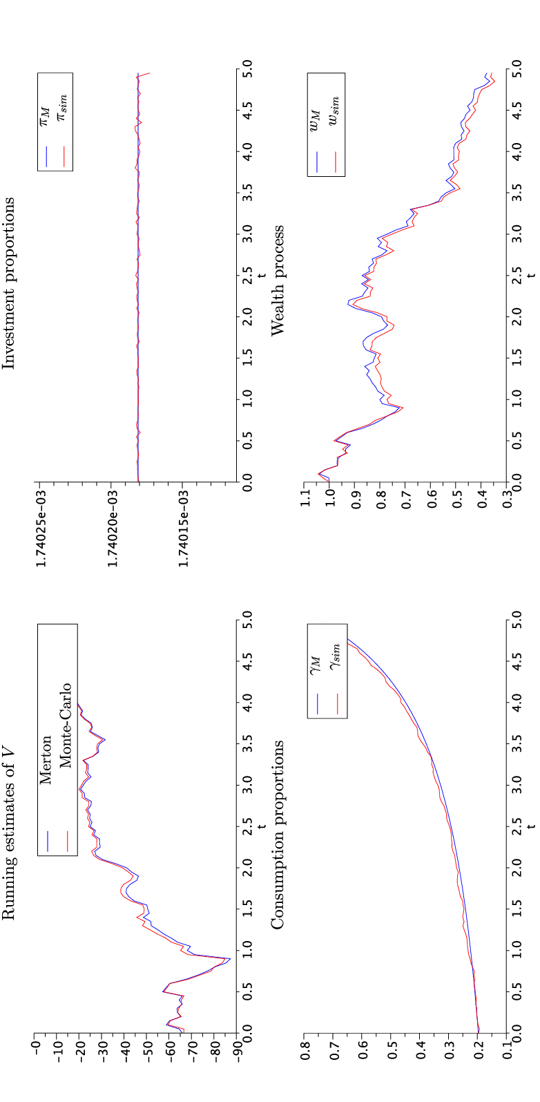
Figure 1 shows the results of the simulation runs for the 3-dimensional version of the problem using paths. The top left panel shows the running estimate of the value function along a particular realization of Brownian motion . The top right and bottom left panels show investment and consumption proportions, respectively. Finally, the bottom right panel depicts the estimated wealth process compared to the Merton wealth process.
As we see, all the graphs give a very satisfactory approximation to the Merton solution. This is especially remarkable taking into account that we are already in dimension , and we have used relatively few paths.
We now present the study of how the accuracy of the solutions to the Merton problem varies for different values of the number of simulations and number of dimensions . We found that the number of time steps used to discretize the integral in (3.2) does not greatly influence the accuracy of the solutions.
We compare the estimates of the optimal starting found by the procedure (2.23) in Algorithm 1. For each test, we keep the initial data of Step fixed. We then run Step of Algorithm 1, each time approximating the function with a different set of Monte Carlo paths. This way, we can investigate how sensitive our optimized values of are to the Monte Carlo procedure for approximating the expectation operator.
Table 3 and Table 4 present the results of the simulations for different number of Monte Carlo paths to calculate , and , respectively. We see that the numerical results work reasonably well for when we choose to use Monte Carlo paths. The average is pretty close to the true value, and the volatility of the estimates stays modest. However, for larger values of , we see that the estimates are either not as accurate, or become more volatile.
For , the results look much better. For , we see a considerable drop in the volatility of the estimates, and all of them lie within two standard deviations of the true value, with most of them being less than one standard deviation away.
These results are very encouraging. They show that, even in dimensions up to , having a reasonably modest number of Monte Carlo paths of can provide satisfactory results when solving the Merton problem. This is particularly interesting since the traditional HJB approach would struggle in these dimensions unless the problem has a particular structure such that we can work out the value function explicitly.
One might think that the accuracy of the method relies on the special structure of the Merton problem. We now show that this is not the case. We consider departures from the basic problem where accurate numerical solutions are available.
| Merton | 9.97 | 9.49 | 8.92 | 8.61 | 8.17 | 8.02 | 7.73 | 7.44 | 7.11 | 6.68 |
| Average() | 9.72 | 9.33 | 8.64 | 8.86 | 7.53 | 7.85 | 7.36 | 7.54 | 6.44 | 5.31 |
| Stdev() | 0.12 | 0.14 | 0.23 | 0.34 | 0.30 | 0.30 | 0.36 | 0.60 | 0.24 | 0.48 |
| Time / run (min) | 0.67 | 2.32 | 2.95 | 3.51 | 4.08 | 4.63 | 5.15 | 5.61 | 6.41 | 6.83 |
| Merton | 10.10 | 9.67 | 9.34 | 8.63 | 8.35 | 8.13 | 7.33 | 7.10 | 6.83 | 6.48 |
| Average() | 10.15 | 9.58 | 9.35 | 8.76 | 8.29 | 8.33 | 7.30 | 7.16 | 6.63 | 6.95 |
| Stdev() | 0.04 | 0.08 | 0.06 | 0.08 | 0.08 | 0.12 | 0.15 | 0.19 | 0.12 | 0.49 |
| Time / run (min) | 6.87 | 22.90 | 28.65 | 34.42 | 40.06 | 46.25 | 52.08 | 57.27 | 61.26 | 68.09 |
4.2 Non-constant relative risk aversion
The example of the Merton problem has shown us that the Monte Carlo method can handle situations where we deal with a multi-dimensional Brownian motion. However, the multiplicative scaling property of the CRRA utility function means that we are unable to assess the accuracy in predicting . The remarkable accuracy in prediction in Figure 1 is caused by the fact that , for some function , and the fact that the optimal satisfies (2.26).
It will therefore be informative the consider an example where the proportion of money invested in the risky assets varies with wealth. This can be done, although the price to pay is dimensionality. In this Section, we assume that the financial market has constant coefficients and that there is only one asset in the market.
For , we define the agent’s marginal utility as
| (4.11) | ||||
| (4.12) |
What this means is that, for small values of wealth , the agent’s relative risk aversion is close to and the agent behaves similarly to the Merton investor from Section (4.1) with , and , and value function . Conversely, the investor for large values of is less risk averse, with risk aversion . He behaves like a Merton investor from Section (4.1) with , , and , and value function .
In dimension one, there are two very effective methods for solving this problem: policy improvement and quantisation77 7 Both of which are difficult to generalise to dimensions more than one, though.. We proceed by briefly describing each one of them, and then by comparing their performance with the Monte Carlo scheme we proposed earlier.
Policy improvement. We follow the approach described in Section of [9]. The HJB equation for our problem is
| (4.13) |
and we are given the terminal value
| (4.14) |
Given functions (4.11), functions and , although not available in closed form, can be found efficiently using binary search.
We therefore give ourselves a grid of time points and a grid of space points and we wish to find evaluated at their mesh.
At the boundaries, we know that the solution resembles the Merton solutions:
| (4.15) |
Let be a functional acting on smooth test functions as
| (4.16) |
Noticing that
| (4.17) | ||||
| (4.18) |
where and , it is possible to approximate acting on by a sparse triagonal matrix acting on a column vector , using approximations (4.17) plugged into (4.16)88 8 Where we consider as a column vector, with the corresponding controls and ..
We now discretize the differential operator appearing in the HJB equation (4.13) on the chosen time and space grid. By letting and , we obtain:
| (4.19) |
We took , giving the Crank-Nicholson method. We define to act on the boundary points and in such a way that (4.19) yields boundary solutions given by (4.15).
Given , (4.19) is then a sparse set of linear equations which we solve for . We then improve on by maximisation in (4.19), given the found . We iterate the process until convergence.
Figure 2 shows the results of the policy improvement algorithm for . As we see, we were able to recover the whole value function using the method described above. It is worth pointing out, though, that the method is tricky to implement even in one dimension, and higher dimensions are almost certainly out of question. However, once has been found in one dimension, working out the optimal consumption and investment around a sample path of Brownian motion are immediate.
Quantization. We proceed to a method which builds on the observations from Section 2, but avoids using the Monte Carlo method for approximating the expectation operator in (2.9). Instead, quantisation proposes approximating the expectation of the Brownian functional by a deterministic sum. Here we follow the details from the website [8] and related papers [7] and [1]. The idea is to use the Karhunen-Loeve expansion of Brownian motion :
| (4.20) |
where is a sequence of independent normal random variables with variance . Here the decomposition functions are
| (4.21) | ||||
| (4.22) |
Brownian motion is then firstly approximated by choosing the first terms in the sum (4.20). We can then think of and as -dimensional vectors, and the Brownian motion as being approximated by the dot product
| (4.23) |
We then quantise the random -dimensional vector by a random variable taking distinct values with respective probabilities , and giving us the final approximation
| (4.24) |
Now, if we need to calculate an expected value of a functional
| (4.25) |
we can now approximate it by a deterministic sum
| (4.26) |
The effectiveness of this application depends on the number of terms taken in the expansion (4.20), as well as the placing of the points and weights and . Files of the points and weights for many different values of and for dimension up to 10 may be freely downloaded from the website [8]. These points and weights are optimal quantizations of the standard Gaussian distribution, in a sense explained in detail there. For a chosen number of , we can therefore load up the optimal and from these files. For our runs, we use .
The important thing is that, for the current problem, the calculations we need to perform are of the particular form (4.25). Indeed, in a complete market with one asset, we have
| (4.27) |
compare it with (2.9). Here has a closed-form expression
| (4.28) |
which is of the required form (4.25).
Having laid out the problem setup and the accurate numerical methods for solving the problem, we now show the numerical results of our calculations.
Comparison of the methods. Figure 3 shows the results of the simulation runs. It is clear that all the methods proposed give virtually the same answers; with Monte Carlo being only away from the two benchmark methods of policy improvement and quantisation. The most reassuring message here is that the Monte Carlo methodology also does a very good job on approximating the investment proportions for the problem as in (2.26) and (2.12). This is the part the the Merton problem example was unable to reveal due to the special structure.
The time taken to get the answer for the policy improvement was approximately minutes, most of which was taken on the calculation of the value function (evaluating the solution along a chosen path is extremely fast). In comparison, quantisation has taken roughly minutes, and Monte Carlo took minutes.
Of course, each of the methods has their costs and benefits. The value function takes a time-investment at the start, but is very fast regardless of how many sample paths we would like to evaluate. This is not the case for quantisation and the Monte Carlo method. Quantisation is the overall speed-winner here, however we must remember that this is mainly due to the preloaded files which we used to quantise the Brownian motion.
Overall, we conclude that the Monte Carlo method performs very well on the complete market problems, as it should. After all, as mentioned before, the only errors we are incurring are numerical: approximating the derivatives and the expectation operator. With sufficient computational power, these should be possible to be made small.
4.3 Incomplete markets driven by a diffusion
Finally, we consider an example where no benchmark methods are available, and the bounds derived in (2.10) are the only sensible indicator for how well our method is doing. We consider an example that is as challenging as possible: an incomplete market driven by a diffusion.
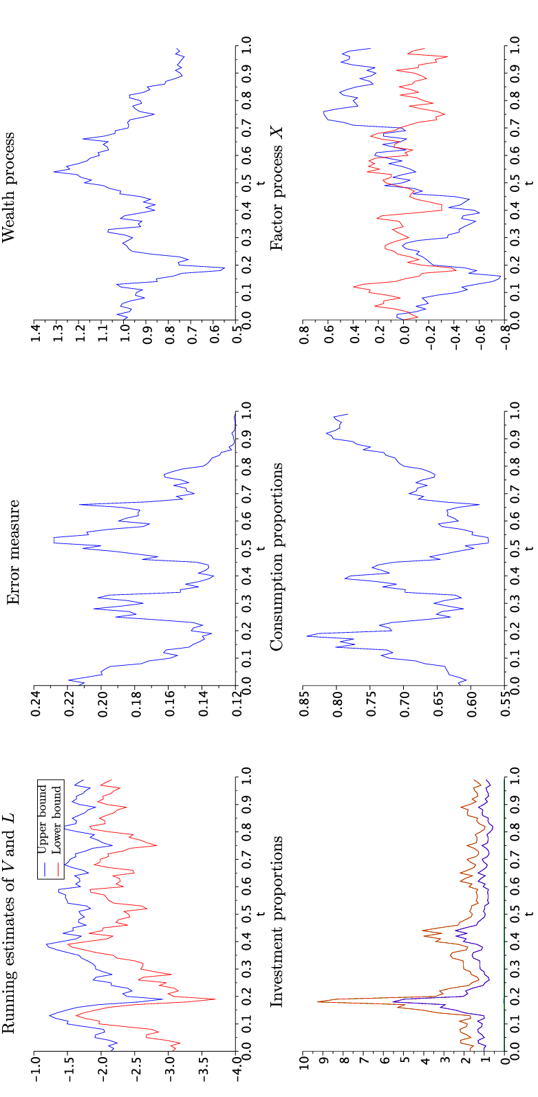
As a specific example, we consider a market composed of stocks driven by a -dimensional Brownian motion. The same Brownian motion drives the -dimensional factor process , which we assume to a be an OU process with the mean-reversion and volatility parameters generated randomly. We take a CRRA utility function, with a number of Monte Carlo paths being equal to . The results of the optimisation run are depicted on Figure 4. The run time here took . The details regarding the parameters are displayed below the panel.
As we can see from the first two panels on the top, the upper and lower bounds stay reasonably close during the sample runs, with the error measure defined in (2.20) between and , and generally decreasing as we near the end of investment.
This is a positive result, especially in light of the dimensionality of the problem. Notice that the market is incomplete, and that the value function for this problem would need to be -dimensional ( dimension for wealth, for time, and for the factor process ). Hence, any other method for approaching this problem would really struggle.
We could of course try to improve on the performance of this algorithm. We lose efficiency when we use the approximation of in (2.13), and also when we truncate the expression (2.22) for . However, our main goal of the paper has already been achieved here: we have illustrated how to use our method on a very difficult problem, and derived satisfactory bounds on the efficiency.
5 Conclusions
This paper presented an effective methodology for tackling optimal investment problems in incomplete markets driven by a Brownian diffusion. We were able to derive a generic methodology for numerically tackling these problems by taking some convenient mode realisation of the market. Secondly, we settle for suboptimal controls which are close to the optimal control.
These assumptions are not a weakness of the method; they are rather a necessary cost needed to be taken if we want to get concrete investment advise in a general setup. After all, they let us derive what we really need in practise: a method for finding a good investment strategy when faced by a particular realisation of the market!
We have also illustrated the effectiveness of the method in a variety of contexts. For the problems where other reliable numerical techniques are available, we showed our method does just as good. For a very complex multi-dimensional problem concluding Section 4, we have showed that the investment errors can be kept satisfactory low. No other method was able to provide even estimates of the solutions in this context. This proves the effectiveness of the method and shows that it has a potential of giving what we really need: concrete investment prescriptions facing a particular market environment.


References
- [1] Corlay, S. Some aspects of optimal quantization and applications to finance. PhD thesis, Université Pierre et Marie Curie, 2011.
- [2] Cox, J. C., and Huang, C.-f. Optimal consumption and portfolio policies when asset prices follow a diffusion process. Journal of economic theory 49, 1 (1989), 33–83.
- [3] Karatzas, I. Optimisation problems in the theory of continuous trading. Control Optim 27 (1989), 1221–1259.
- [4] Karatzas, I., Lehoczky, J. P., and Shreve, S. E. Optimal portfolio and consumption decisions for a “small investor” on a finite horizon. SIAM journal on control and optimization 25, 6 (1987), 1557–1586.
- [5] Merton, R. Lifetime portfolio selection under uncertainty: the continuous-time model. Rev. Econ. Statist., 51 (1969), 247–257.
- [6] Merton, R. Optimum consumption and portfolio rules in a continuous-time model. J. Econ. Theory, 3 (1971), 373–413.
- [7] Pagès, G., and Printems, J. Optimal quadratic quantization for numerics: the Gaussian case. Monte Carlo Methods and Applications 9 (2003), 135–166.
- [8] Pagès, G., Printems, J., and Corlay, S. The optimal quantization web site. http://www.quantize.maths-fi.com/gaussian_process_database; accessed 20-March-2013.
- [9] Rogers, L. C. G. Optimal Investment. Springer Briefs in Quantitative Finance. Springer-Verlag, 2013.
- [10] Rogers, L. C. G., and Williams, D. Diffusions, Markov Processes and Martingales, vol. 2. Cambridge University Press, 2000.