Computational error estimates for Born-Oppenheimer molecular dynamics with nearly crossing potential surfaces
Abstract.
The difference of the values of observables for the time-independent Schrödinger equation, with matrix valued potentials, and the values of observables for ab initio Born-Oppenheimer molecular dynamics, of the ground state, depends on the probability to be in excited states and the electron/nuclei mass ratio. The paper first proves an error estimate (depending on the electron/nuclei mass ratio and the probability to be in excited states) for this difference of microcanonical observables, assuming that molecular dynamics space-time averages converge, with a rate related to the maximal Lyapunov exponent. The error estimate is uniform in the number of particles and the analysis does not assume a uniform lower bound on the spectral gap of the electron operator and consequently the probability to be in excited states can be large. A numerical method to determine the probability to be in excited states is then presented, based on Ehrenfest molecular dynamics and stability analysis of a perturbed eigenvalue problem.
Key words and phrases:
Landau-Zener probability, Egorov’s theorem, Born-Oppenheimer approximation, WKB expansion, microcanonical ensemble, Ehrenfest dynamics, ab initio molecular dynamics.1. Motivation for error estimates in ab initio molecular dynamics
Molecular dynamics is a computational method to study molecular systems in materials science, chemistry and molecular biology. The simulations are used, for example, in designing and understanding new materials or for determining biochemical reactions in drug design [14].
The wide popularity of molecular dynamics simulations relies on the fact that in many cases it agrees very well with experiments. Indeed when we have experimental data it is often possible to verify the correctness of the method by comparing with experiments at certain parameter regimes. However, if we want the simulation to predict something that has no comparing experiment, we need a mathematical estimate of the accuracy of the computation. In the case of molecular systems with few particles, such studies are made by directly solving the Schrödinger equation. A fundamental and still open question in classical molecular dynamics simulations is how to verify the accuracy computationally, i.e., when the solution of the Schrödinger equation is not a computational alternative.
The aim of this paper is to determine quantitative error estimates for molecular dynamics, including the case with nearly crossing electron potential surfaces that can yield large errors, without solving the Schrödinger equation but by combining mathematical stability analysis of eigenvalue problems with quantitative numerical Ehrenfest molecular dynamics computations of perturbations. Having molecular dynamics error estimates opens, for instance, the possibility of systematically evaluating which density functionals or empirical force fields are good approximations and under what conditions the approximation properties hold. Computations with such error estimates could also give improved understanding of when quantum effects are important and when they are not, in particular in cases when the Schrödinger equation is too computationally complex to solve.
The first step to check the accuracy of a molecular dynamics simulation is to know what to compare with. Here we compare the value of any observable , of nuclei positions , for the time-independent Schrödinger eigenvalue equation, , with the corresponding molecular dynamics observable, defined by a Hamiltonian , the wave function and the eigenvalue . The approximation error we study is therefore the microcanonical setting
| (1.1) |
based on a molecular dynamics path , with total the energy equal to the Schrödinger eigenvalue . The inner product is defined in , where corresponds to discrete (electron) states. The observable can for instance be the local potential energy, used in [50] to determine phase-field partial differential equations from molecular dynamics simulations. For the sake of simplicity we first explain the basic idea for observables depending only on position variables . The general case of position and momentum dependent observables is treated in Section 2 using the Weyl quantization. The time-independent Schrödinger equation has a remarkable property of accurately predicting experiments in combination with no unknown data, thereby forming the foundation of computational chemistry. However, the drawback is the high dimensional solution space for nuclei-electron systems with several particles, restricting numerical solution to small molecules. In this paper we study the time-independent setting of the Schrödinger equation as the reference. The proposed approach has the advantage of not requiring any initial data as input, on the other hand, an assumption on convergence rates of time averages of molecular dynamics observables is needed.
The second step to check the accuracy is to derive error estimates. We have three types of error: time discretization error, sampling error and modeling error. The time discretization error comes from approximating the differential equation for molecular dynamics with a numerical method, based on replacing time derivatives with difference quotients and time steps . The sampling error is due to truncating the infinite and using a finite value of in the integral in (1.1). The modeling error (also called coarse-graining error) originates from eliminating the electrons in the Schrödinger nuclei-electron system and replacing the nuclei dynamics with their classical paths; this approximation error was first analyzed by Born and Oppenheimer in their seminal paper [4].
The time discretization and truncation error components are in some sense simpler to handle by comparing simulations with different choices of and , although it can, of course, be difficult to know that the behavior does not change with even smaller and larger due to metastability, see [30, 7]. The modeling error is more difficult to check since a direct approach would require to solve the Schrödinger equation. Currently the Schrödinger partial differential equation can only be solved with few particles, therefore it is not an option to solve the Schrödinger equation in general. The reason for using molecular dynamics is precisely to avoid solving the Schrödinger equation. Consequently, the modeling error requires mathematical error analysis. Egorov’s theorem, cf. [39, 5], provides such error estimates and is used also here. However, in the literature there seems to be no error analysis that is precise, simple and constructive enough so that a molecular dynamics simulation can use it in practice to assess the modeling error also in the case when the electron operator has eigenvalues (i.e., potential surfaces) which are not well separated and may cause large modeling error. For instance, crossing eigenvalue surfaces can form so called conical intersections, which provide the mechanism for many chemical reactions, see [47, 51]. If the excited electron energy levels are well separated from the ground state energy, molecular dynamics based on the ground state energy is a good approximation, as first analyzed by Born and Oppenheimer [4]. On the other hand, in a quantum system with two electron energy levels that are not well separated, the dynamic transition probability from one state to the other state for a moving particle can be substantial, as determined by Landau and Zener [53] and generalized to a similar dynamic case in two space dimensions in [27]. We denote the transition probability to go from the ground state to excited states for a time-dependent problem ”dynamic transition probability”, as in the Landau-Zener model, to distinguish it from the ”probability to be in excited states” for the time-independent Schrödinger eigenvalue problem.
Our alternative error analysis presented here relates computable dynamic transition probabilities to the probability to be in excited states for the time-independent Schrödinger equation and is developed with the aim to give a different point of view that could help to construct algorithms that estimate the modeling error in molecular dynamics computations. Our analysis differs from previous ones by combining analytical estimates with computations and it is based on three main steps:
- -
analyzing the time-independent Schrödinger equation as the reference model, including excited electron states with near crossing potential surfaces and the accuracy of observables as a function of the probability to be in excited states (in Section 2),
- -
studying stochastic molecular dynamics, constrained to the manifold of constant energy, based on small stochastic perturbations of the standard Born-Oppenheimer Hamiltonian dynamics,
- -
using stability analysis of a perturbed eigenvalue problem to estimate the probability to be in excited electron states, based on perturbations related to (Landau-Zener like) dynamic transition probabilities (in Section 3),
- -
applying Ehrenfest molecular dynamics to computationally estimate the dynamic transition probabilities (in Section 4).
The estimation method is tested on one and two dimensional problems but to conclude how useful the method is for realistic chemistry problems will require more work.
The next section introduces the Schrödinger and molecular dynamics models and ends with a more detailed outline.
1.1. The Schrödinger and molecular dynamics models with an outline of the main results
In deriving the approximation of the solutions to the full Schrödinger equation, the heavy particles are often treated within classical mechanics, i.e., by defining the evolution of their positions and momenta by equations of motions of classical mechanics. Therefore we denote by the time-dependent function of the nuclei positions, with time derivatives denoted by
We denote the Euclidean scalar product on by
Furthermore, we use the notation , and as customary . The notation is also used for complex valued functions, meaning that holds uniformly in for .
The time-independent Schrödinger equation
| (1.2) |
models many-body (nuclei-electron) quantum systems and is obtained from minimization of the energy in the solution space of wave functions, see [42, 41, 2, 46, 29, 6]. It is an eigenvalue problem for the energy of the system, described by the Hamiltonian operator
| (1.3) |
where denotes the identity matrix, and by the wave functions, , belonging to a set of permissible electron states which we assume, for simplicity, to be finite, . We use a normalized solution and without loss of generality we assume that all nuclei have the same mass . If this is not the case, we can introduce new coordinates , which transform the Hamiltonian to the form we want . In computational chemistry, the electron operator Hamiltonian , is independent of and it is precisely determined by the sum of the kinetic energy of electrons and the Coulomb interaction between nuclei and electrons. The wave function is then in a subspace of , with electron coordinates , see [29]. By introducing a finite dimensional basis of the electron solution space, minimization of the energy under the constraint leads to the eigenvalue problem (1.2) for the solution , with the matrix defined by the matrix components and . To be able to compute with several electrons, i.e. , the electron solution space is often simplified in the form of Hartree-Fock or density functional approximations, which also lead to eigenvalue problems which now are non linear, see [29]. We assume that the electron operator is linear and self-adjoint, in a finite dimensional complex valued Euclidian space (for simplicity), with the usual inner product , and acts as a matrix multiplication. An essential feature of the partial differential equation (1.2) is the high computational complexity of finding the solution in a subset of the Sobolev space . The mass of the nuclei, , are much greater than one (electron mass).
In contrast to the Schrödinger equation, a molecular dynamics model of nuclei , with a given potential , can be computationally studied for large by solving the ordinary differential equations in the fast time scale. We will use the slow time scale with positions and scaled momenta satisfying
| (1.4) |
In the slow time scale the nuclei move in unit time, since . This computational and conceptual simplification motivates the study to determine the potential and its implied accuracy compared with the the Schrödinger equation, as started already in the 1920’s with the Born-Oppenheimer approximation [4]. The purpose of our work is to contribute to the current understanding of such derivations by showing convergence rates under new assumptions. The precise aim in this paper is to estimate the error
| (1.5) |
for scalar smooth observables of the time-indepedent Schrödinger equation (1.2) approximated by the corresponding molecular dynamics observable , which is computationally cheaper to evaluate in the case with several nuclei; Section 2 includes also the general case with position and momentum dependent observables.
The main step to relate the Schrödinger wave function and the molecular dynamics solution is the so-called zero-order Born-Oppenheimer approximation, where solves the classical ab initio molecular dynamics (1.4) with the potential determined as an eigenvalue of the electron Hamiltonian for a given nuclei position . That is, and
| (1.6) |
for a normalized electron eigenvector (here the ground state). The initial data is chosen to have its energy equal to the eigenvalue , i.e. . The Born-Oppenheimer expansion [4] is an approximation of the solution of the time-independent Schrödinger equation which is shown in [17, 25] to solve the time-independent Schrödinger equation approximately when the electron operator have eigenvalues that are well separated, satisfying
| (1.7) | for a positive constant independent of . |
This expansion, analyzed by the methods of multiple scales, pseudo-differential operators and spectral analysis, e.g., in [16, 17, 25, 13], can be used to study the approximation error (1.5). The work [16, 17, 25, 31] prove asymptotic expansions for the eigenfunction. In the literature one can also find precise statements on the error for the setting of the time-dependent Schrödinger equation, e.g., in [31, 5, 35, 26], which in some sense is easier since the stability issue is more subtle in the eigenvalue setting. The aim of our work is to present a method to analyze this stability of the eigenvalue problem, using the dynamic transition probability estimated from Ehrenfest dynamics simulations as quantitative input, without assuming an -uniform lower bound on the spectral gap.
We present error estimates for molecular dynamics approximation of time-independent observables in quantum mechanics, valid also when the eigenvalues of the electron operator may nearly intersect and thereby increase the probability of being in excited states. For the Schrödinger solution to (1.2), with the electron ground state satisfying (1.6), the probability to be in excited states is
| (1.8) |
where . The derivation of the approximation error is divided into three steps which defines the outline of the paper:
- I.
The first step, in Section 2, proves that observables based on the time-independent Schödinger equation can be approximated by stochastic molecular dynamics on the constant energy manifold. The convergence rate depends on the nuclei/electron mass ratio and the probability to be in excited states. The proofs use Egorov’s theorem and assume that the expected value of space-time averages of the molecular dynamics observable converge in distributional sense with a rate related to the maximal Lyapunov exponent.
- II.
The second step, in Section 3, presents a numerical method to determine the probability to be in excited states from stability analysis of a perturbed eigenvalue problem. The perturbation is determined from a time-dependent excitation problem related to the Landau-Zener model (with denoting the dynamic transition probability to go to the excited state). Resonances of the eigenvalue problem then determines the larger probability (to be in excited states for the Schrödinger eigenvalue problem) from the perturbations in the dynamic problem.
- III.
The final step, in Section 4, on numerical results, illustrate that the dynamic transition probability can be determined from Ehrenfest molecular dynamics simulations applied to two simple model problems.
Section 5 proves a lemma on the regularity of the expected value of the molecular dynamics solution and establishes in three other lemmas estimates on remainder terms in Moyal expansions used in the theorems. Section 6 formulates WKB solutions in the case with caustics.
The main ingredient in step I is Egorov’s theorem which has been used extensively to study semiclassical limits both in the time-dependent and time-independent case, cf. [39, 5, 44]. We derive two estimates: Theorem 2.1 proves an estimate of a weighted difference of the Schrödinger and molecular dynamics observables and Theorem 2.2 derives an estimate of the difference of the Schrödinger and molecular dynamics observables, without the weight. The idea to assume ergodic classical dynamics to prove convergence of observables, in [43, 28], initiated the activity on quantum ergodicity [52] and related results on semiclassical limits for scalar potentials, [20], and matrix potentials with distinct eigenvalues [3]. The work [44] includes a recent review of semiclassical limit results in the case of well separated electron eigenvalue surfaces. In this case with well separated electron eigenvalues, satisfying (1.7), the probability to be in the excited state is proved to be small . We want to include the case when molecular dynamics simulations become inaccurate in practice. For an actual molecular dynamics simulation the mass is given and the electron potential does not depend in , so a positive spectral gap does not depend on . However, if the mass is not large enough the molecular dynamics approximation may be inaccurate. Our analysis is asymptotic for large and to include the situation with a small gap for a certain mass we therefore consider a model when the spectral gap
| (1.9) |
can be close to zero, i.e. when it is not uniformly bounded from below with respect to , and then can be large as seen e.g. in the Landau-Zener probability (3.10) and Figure 4. There are four main new ingredients in our theorems compared to previous studies. It is well known that the standard proof of Egorov’s theorem, in the time-dependent case, combined with an assumption on the molecular dynamics convergence rate towards its ergodic limit yields an error estimate for the molecular dynamics observables as compared to the Schrödinger observables. The precise form of the assumption on the convergence to the ergodic limit is important for the conclusion of the approximation error compared to Schrödinger observables: (1) for instance, assuming an algebraic convergence rate , for molecular dynamics time-averages of length , would only give logarithmic error estimates (also in the case with a uniform spectral gap); (2) it is difficult to verify ergodicity for Hamiltonian dynamics, both theoretically and numerically. The first new ingredient here is to use stochastic dynamics constrained on the constant energy surface instead of Hamiltonian dynamics. Introducing small stochastic perturbations on the constant energy manifold have the advantage to guarantee ergodicity with respect to the microcanonical ensemble and to provide observables with higher regularity. Our second ingredient is to use a more precise convergence rate assumption based on space-time averages, which can be tested numerically (see Figure 10) and yields a better error estimate , for a positive , The third ingredient is to prove uniform convergence rates in the number of particles by careful use of localized mollifiers. Previous convergence proofs require for instance, for a certain constant , the quantity to be small but typically this is a large number for systems with many particles unless the mass ratio is very large and increasing with the number of particles , see [20] and Theorem 15.4 in [54]. The fourth ingredient is that we include non uniformly spectral gap bounds (1.9): Theorems 2.1 and 2.2 prove the error estimate in step I in terms of the probability to be in excited states, which is not a typical a priori information. Consequently the computational approximation of in steps II and III is an important complement. Although to evaluate the practical value of the suggested method to estimate the computational error in molecular dynamics these two steps need to be tested on more realistic chemistry problems.
The alternative to consider molecular dynamics at constant temperature using the canonical ensemble is important in practice and it also has the advantage of proved ergodic limits. The canonical ensemble is in a sense the average of the microcanonical ensemble over all energies weighted with the Gibbs density. Therefore the results here are useful for ongoing analysis in the constant temperature setting.
2. Molecular dynamics approximation of Schrödinger observables for matrix-valued potentials
For every mass , we consider wave functions and eigenvalues , solving the Schrödinger eigenvalue equation
| (2.1) |
where
| (2.2) |
Here, the symmetric smooth matrix valued potential has (electron) eigenvalues , ordered increasingly, with normalized eigenvectors satisfying
and the spectral gap condition (1.9). The eigenvalues may be degenerate but is not. Both and depend on the mass and we will only consider those eigenfunctions where the corresponding eigenvalue is bounded, i.e., the for which as . That is, we assume that for every there are solutions with eigenvalue to (2.1), as . On the other hand, the matrix does not depend on explicitly and consequently also the eigenvectors and eigenvalues and do not depend on explicitly. However to include the case of a small spectral gap, we assume that the positive spectral gap, , in (1.9) is not uniform in and we study estimates depending on the two parameters and . To handle ergodicity for the Born-Oppenheimer dynamics, we will below assume that the smallest eigenvalue is smooth and tends to infinity as . This assumption in fact also implies that the spectrum of is discrete, see [9].
We consider a given smooth scalar observable in the Schwartz space constructed as
| (2.3) |
where for some the mollifier is defined by and is smooth and compactly supported. We assume that each solution to (2.1) is normalized, i.e. , and define for each the observable
| (2.4) |
based on the Weyl quantization, see [32],
using the inner products
We note that in the case is a function of only, then the Weyl quantization acts as a multiplication operator, i.e. . We also define the Wigner transform
| (2.5) |
and
and note that is different for different eigenvalues . The change of variables
shows that for any and
Our estimates of remainder terms use the corresponding function defined for by
| (2.6) |
which is the ”Wigner”-function corresponding to the alternative quantization
| (2.7) |
We will approximate the Schrödinger observable by dynamics related to ab initio molecular dynamics
| (2.8) |
based on the Hamiltonian
We assume that is smooth and coercive in the sense that
| (2.9) |
In order to obtain precise estimates of the approximation error which are uniform in we consider a mollified Hamiltonian
where is a standard mollifier on the small scale . To obtain good approximation of observables compared to the Schrödinger case we use . To ensure ergodic molecular dynamics and still approximate the Born-Oppenheimer dynamics we will compare the Schrödinger observable to the observable for stochastic dynamics restricted to the manifold
for the constant energy equal to the Schrödinger eigenvalue, with a small stochastic perturbation of (2.8). Let denote the phase space variable, then one example of such stochastic Stratonovich dynamics on takes the form
| (2.10) |
where is a small positive parameter, is the standard Wiener process in with independent components, the skew symmetric matrix is defined by , the parameter is positive, and the projection onto the tangent space of at reads
with the normal to . We assume that for all . Since also is assumed to be smooth and coercive, the set is a smooth compact codimension one manifold in for every . The dynamics (2.10) is the projection of the Ito differential equation
| (2.11) |
to and has a unique equilibrium measure, which is the Gibbs measure
The diffusion parameter can, for instance, also be a semi-positive definite constant diagonal matrix, so that (2.11) includes the Langevin equation. The work [12] proves that the projected dynamics (2.10) also is ergodic and the equilibrium measure is the microcanonical measure
i.e. where is the surface measure on induced by the Lebesgue measure in . Alternative ergodic dynamics on sampling the microcanonical measure are presented in [12].
The Ito dynamics corresponding to (2.10) reads, see [12] and [8],
| (2.12) |
where is the mean curvature at on . The Kolmogorov equation for the expected value , for , of paths satisfying (2.10) becomes
| (2.13) |
where denotes the Hessian with respect to , so that
This Kolmogorov equation has an intrinsic definition based only on the coordinates on , see [12]. The expected value is smooth and the compact support of implies that decays rapidly as , so that is in the Schwartz class. The work [12] also proves an exponential convergence rate to equilibrium: let the initial data be smooth in a neighborhood of then there is a positive constant such that
| (2.14) |
The upper and lower bounds in [21] on the convergence rate exponent for Langevin dynamics in the full phase space prove that the rate is bounded from below by a constant times and from above by a constant times where is the damping factor, as in (2.11), for fixed positive temperature .
Let , for be the stochastic flow of the dynamics (2.10), i.e. the solution that starts in at time , for a realization of the Wiener process. Then we have . We write so that . This function satisfies the exponential growth
| (2.15) |
where is independent of , and , as derived in Lemma 5.1 under assumption (5.3) including weak near crossing of eigenvalues.
Define the molecular dynamics microcanonical observable
| (2.16) |
depending on the initial energy . Our main assumption on the dynamics is that we assume that for some there is a positive constants , independent of and , such that
| (2.17) |
The constant depends on the observable so that an observable related to a macroscopic quantity may have better convergence rate in the case of a large system.
From (2.14) we know that there is a constant satisfying (2.17). Assumption (2.17) says that the decay with respect to time of
integrated over the Wigner distribution is exponential with the decay rate (for some and ) plus possibly an additional constant small term independent of . The ergodic assumption
for the Hamiltonian dynamics with is used in [43, 28], [20] and [3] to prove convergence of Schrödinger observables. This ergodic assumption is difficult to verify numerically, since a numerical approximation of the dynamics will always perturb the dynamics and it is theoretically unclear how this perturbation effects the dynamics over infinite time, see [49]. To find a method to prove ergodicity for general Hamiltonian systems also remains a challenge, cf. [49]. An advantage with assumption (2.17) is that it can be tested numerically for some initial points , see Figure 10, since the time discretization error can be made small compared to the bound , by taking a small time step , and the simulation time is finite. Not all dynamics satisfy (2.17). For instance there exists billiard dynamics in ”stadium” domains in that is proven to be ergodic for almost all initial data but is non ergodic for some data with corresponding concentrated Schrödinger eigenfunctions, see [19]. Small perturbations of this data with non ergodic dynamics will need very long time to reach asymptotically ergodic behavior and consequently also the stochastic regularization above is likely to have in (2.17) depending on so that our assumption would not hold.
Having introduced the necessary notation and terminology, we are now ready to present an estimate for the weighted difference between the Schrödinger and stochastic molecular dynamics observables that is expressed in terms of the spectral gap, the mass and the excitation probability. Theorem 2.2, presented in the end of this section, then estimates the difference of the observables without the weight.
Theorem 2.1.
For every consider the Schrödinger eigenvalue problem (2.1)-(2.2) with a solution , for a corresponding eigenvalue , and assume:
- (i)
the observable satisfies (2.3) and the potential is smooth with bounded, uniformly in , where is the matrix -norm in ,
- (ii)
- (iii)
the electron eigenvector and eigenvalue are smooth and have bounded derivatives satisfying, for some defined in (1.9) (which may depend on ) and any , and for any ,
- (iv)
the Hamiltonian is smooth, satisfies the coercivity (2.9) and for all ,
- (v)
the exponential bound (2.15) holds with the constant uniformly bounded in .
Let the probability to be in excited states be denoted by , as defined in (1.8), and define the Wigner transform by (2.5). Then, for , the molecular dynamics observable approximates the Schrödinger observable , defined in (2.4), with the weighted error estimate
| (2.18) |
for any , and by choosing such that , and sufficiently small
| (2.19) |
for a constant , independent of , , and .
To prove this theorem, we modify the proof of Egorov’s theorem [39] to include stochastic dynamics and the assumption (2.17) on the space-time convergence rate and to replace the uniform spectral gap bound for matrix valued perturbation potentials , in [3, 44], with Assumption (iii). Assumption (iii) with excludes a conical intersection but avoided crossings are allowed with a spectral gap in (1.9) that is not uniformly bounded from below as a function of . The Landau-Zener probability (3.10) in Section 3.2 (combined with (3.12) and (3.42)) illustrate for instance that can be close to one for an avoided crossing, with a small spectral gap . That can be of the same order as in the estimate (2.18) motivates the study of the approximation error as a function of and . To have large seems to require smaller gaps , see Section 3. It would be desirable to have analytic estimates of , since it is determined by and . Such estimates are known, as , for the case when spectral gap is uniformly bounded from below while in the case with no uniform spectral gap the required smoothness of projection to the ground state is assumed, see [48]. The lack of analytic estimates of is our motivation for using in addition to as parameter in the Theorems and presenting the computational method to determine in this work.
We note that stochastic dynamics has a regularizing effect since , with , is in general more regular than , with . In fact, we do not explicitly need the stochastic flow : the proof only uses the deterministic value and its flow , for , with the generator . The exponential bound in assumption (v) is proved in Lemma 5.1 under an assumption that allows weak near crossing of eigenvalues away from regions where vanishes.
Proof.
Consider the solution operator of the time-dependent Schrödinger equation
defined by . We will compare the observable
to the expected value
By construction we have that is in the compact manifold . The coercivity (2.9) of and the decay of in phase space imply therefore that decays sufficiently fast for large . The integrals above are therefore well defined. Since is smooth, elliptic regularity implies that the solution to the Schrödinger eigenvalue problem also is smooth. Let be the solution to
| (2.20) |
then and . We have, using the commutator and that ,
| (2.21) |
In the fourth equality we have used (2.20) to conclude that
Here the estimate
| (2.22) |
follows by Lemma 5.4 and we note that the term is negligible small by choosing sufficiently small, although the constant typically is large as it depends on order derivatives of the symbol.
To estimate terms in the error representation (2.21) is now the remaining four steps in the proof.
1. The Moyal expansion for the commutator of two Weyl operators in [5, 25] and Lemma 5.5 is stated for scalars and here we apply Lemma 5.5 to each matrix component of to obtain
| (2.23) |
for the matrix components
where the remainder takes the form, see [5] and Section 5,
| (2.24) |
and is smooth. We will use for . Lemma 5.5 in Section 5 shows that
| (2.25) |
3. We have the desired quantity in the left hand side above by adding and subtracting the molecular dynamics observable , to the second term in the left hand side, and using its convergence rate from (2.17) as follows
which yields the last term in the error bound (2.18).
4. It remains to estimate the first term in the right hand side of (2.26). The rule for the composition of Weyl quantizations, cf. [32] and Lemma 5.5 in Section 5,
| (2.27) |
for smooth scalar functions . The first term in the right hand side of (2.26) can be written
and to estimate this term we use (1.8) and write , where and , for , defines the projection onto the ground state. The integral terms including the factor is bounded using Lemma 5.5
The main term related to the consistency of the approximation can be written as follows
where Lemma 5.3 shows that the last term is bounded by
since the symbol satisfies
The next result shows that the difference of the observables can be estimated without the weight .
Theorem 2.2.
Let and assume that
- (i)
the assumptions in Theorem 2.1 hold, and
- (ii)
the function is defined by
then
and
where
Proof.
The function can be written as the convolution
| (2.29) |
and as
Using the assumption that does not vanish, the function is smooth since we have for
and similarly for higher order derivatives.
Taylor expansion implies
for some between and satisfying , and integration with yields the moment relation
| (2.30) |
The definition of shows the error estimate
| (2.31) |
since .
3. Determining the probability to be in excited states
The purpose of this section is to describe a numerical method to approximate the probability to be in excited states for the Schrödinger eigenvalue problem, without solving a Schrödinger eigenvalue problem and instead analyze a certain eigenvalue problem with respect to perturbations related to the dynamic behavior for a time dependent problem. This perturbation study is formal in the sense that precise conditions for its validity is not presented here. The perturbation model is first formulated in one spatial dimension and then in multiple dimensions in Section 3.3. The perturbation uses the WKB-method to formulate transitions and is presented in Section 3.1. The dynamic problem is related to the Landau-Zener model and Ehrenfest dynamics as described in Section 3.2.
3.1. Construction of WKB-solutions
To construct a numerical method for approximating the probability to be in excited states, without solving a Schrödinger equation, we will use a decomposition of the Schrödinger solution into WKB-functions (3.38). This section presents a construction of such WKB-functions.
The singular perturbation of the matrix valued potential in the Hamiltonian (1.3) introduces an additional small scale of high frequency oscillations, as shown by a WKB-expansion, see [36, 23, 34]. We shall construct solutions to (1.2) in such a WKB-form
| (3.1) |
where the amplitude function is complex valued, the phase is real valued in the classically allowed region (and purely imaginary elsewhere, see Remark 3.1), and the factor is introduced in order to have well-defined limits of and as . Note that it is trivially always possible to find functions and satisfying (3.1), even in the sense of a true equality. Of course, the ansatz only makes sense if and do not have strong oscillations for large . The standard WKB-construction [33, 34] is based on a series expansion in powers of , which solves the Schrödinger equation with arbitrarily high accuracy. Instead of an asymptotic solution, we introduce an actual local solution based on a time-dependent Schrödinger transport equation. This transport equation reduces to the formulation in [33].
3.1.1. A WKB-solution
The WKB-function (3.1) satisfies the Schrödinger equation (1.2) provided that
| (3.2) |
We shall see that only eigensolutions that correspond to dynamics without caustics correspond to such a single WKB-mode, as for instance when the eigenvalue is inside an electron eigenvalue gap. Solutions in the presence of caustics use a Fourier integral of such WKB-modes, see [33] and Appendix 6. The purpose of the phase function is to generate an accurate approximation in the limit as . A possible definition, see [33], is the Hamilton-Jacobi equation, also called the eikonal equation
| (3.3) |
The solution to the Hamilton-Jacobi eikonal equation can be constructed locally from the associated Hamiltonian system
| (3.4) |
through the characteristics path satisfying . For the time being, we fix some and vary over a hyperplane (denoted by ) in orthogonal to , see Figure 1. Hence, the trajectories can (locally) cover the space. Later on, in Section 3.3 we shall argue that a superposition of such solutions actually allows us to reconstruct the true (local) solution of the Schrödinger equation. In particular, we will solve the system (3.4) not just once, but for all different .

The amplitude function can be determined by requiring the ansatz (3.1) to be a solution to (3.2), which gives
Thus by using (3.3) we have
| (3.5) |
The usual method for determining from this so-called transport equation uses an asymptotic expansion , see [17, 25]. An alternative is to write it as a Schrödinger equation, as in [33]: we apply the characteristics in (3.4) to write
and define the weight function by
| (3.6) |
and the variable . Then the transport equation (3.5) becomes a Schrödinger-type equation
| (3.7) |
As (3.7) is (formally) a time-dependent Schrödinger equation, we need to impose initial conditions. Once more, we refer to Section 3.3 for a detailed discussion of this subtle issue.
The last step in the construction of the WKB system is to patch together the different trajectories obtained in (3.4)–(3.7). A priori, , , and are functions of , for and , where was a hyperplane in . By uniqueness of solutions to (3.4), the map is locally injective. Considering in addition to , we obtain that is locally invertible. Hence, we may also interpret the functions , , as functions of the space variable alone. Abusing notation, we set , , for in a neighborhood of .
In conclusion, equations (3.3)-(3.7) determine the WKB-ansatz (3.1) to be a local solution to the Schrödinger equation (1.2) in the following sense. Assume that the Hamilton-Jacobi equation has a solution in a domain . Let and , then solves the Hamiltonian system (3.4), for such that . Then
| (3.8) |
solves (1.2) in , since both (3.3) and (3.5) are satisfied and consequently also (3.2). It is well known that Hamilton-Jacobi equations in general do not have global solutions, due to -paths that collide and generate blow up in . However if the domain is small enough and the data on the boundary is compatible (in the sense that on the boundary), noncharacteristic (in the sense that the normal derivative on the boundary) and is smooth, then the converse property holds, i.e. the characteristics generate a local solution to the Hamilton-Jacobi equation, see [11]. Maslov’s method to find a global asymptotic solution by patching together local solutions is described in [33].
Remark 3.1.
In the classically forbidden region we can apply the same WKB method by replacing the phase function by the imaginary phase . The Eikonal equation becomes , which then has a solution, and the transport equation becomes real valued
The matrix is positive semi-definite, so that remains bounded for bounded time and approaches the ground state . In the classical region we instead use the oscillatory behavior to conclude that tends to the ground state, see [1].
3.2. The Landau-Zener model, transition probabilities and Ehrenfest dynamics
Notice that the parameter in (3.4) – (3.7) is just a numerical parameter, which, prima facie, has no connection with physical time. Indeed, we are working in a time-independent setting after all. On the other hand, if is interpreted as time, (3.7) corresponds to a time dependent Schrödinger equation, and we may ask for dynamic transition probabilities of the time-dependent model, denoted by and rigorously defined in (3.12). It turns out below that the time-dependent transition probabilities are easier to analyze than the time-independent ones, , at least under some simplifying assumptions. The link between the time-dependent transition probabilities and the time-independent is not trivial and will be explored in detail in Section 3.3. To have some intuition, it might be helpful to think of as a “local” excitation probability around , with the idea that , in turn, is given as a time/space average of .
We start our discussion by looking at a simple special case of (3.7), the Landau-Zener model, for which the first results on transition probabilities with crossing or nearly crossing electron potentials were obtained. It is given by
| (3.9) |
with a wave function , constant positive parameters and initial data . The transition probability
| (3.10) |
is the so-called Landau-Zener probability, determined using Weber functions in [53] and illustrated in Figure 8. In this particular model, we note that .
In the context of (3.4)–(3.7), the Landau-Zener model can be seen as a special case of
| (3.11) |
which by the WKB-method (3.8) determines a Schrödinger WKB-solution locally and hence the transition probability
| (3.12) |
using the initialization for , where the inflow domain is given by
| (3.13) |
for a given point and the ground state is defined in (1.6). By neglecting the small term in the transport equation (3.11) and using the simplification with the potential and
| (3.14) |
we obtain the Landau-Zener model. The Landau Zener model was constructed to model and explain the dynamic transitions from the ground state to an excited state when the electron potential surfaces cross or nearly cross (with a minimal distance ) and the eigenstates change rapidly (near for small values of ): the eigenvalues of in (3.14) are and the eigenvectors
Remark 3.2.
3.2.1. Ehrenfest dynamics
As far as computations are concerned, the system (3.11) is still very demanding due to the Laplacian on the right hand side. A further simplification mainly introduced for computational reasons (and used in the computational examples of this paper) is the so-called Ehrenfest dynamics
| (3.15) |
which is an approximate WKB solution, by neglecting the small term in the transport equation and replacing the Eikonal equation with , as in [1]. If we write the wave function in its real and imaginary parts , and use initial data that satisfy , then the Ehrenfest dynamics (3.15) is a Hamiltonian system with the Hamiltonian
| (3.16) |
using the primal variables and , the dual variables and . If the probability, , to be in the excited state is small (using the projection in (1.8)) the Ehrenfest Hamiltonian is close to the Born-Oppenheimer Hamiltonian .
3.3. An estimate of the probability to be in excited states for matrix-valued potentials
This section presents a formal stability study of a perturbed eigenvalue problem that provides an approximation for the probability to be in excited states, . The two ingredients are first to determine the perturbation as a dynamic transition problem, related to the Landau-Zener model, and thereafter to use the stability analysis of a matrix eigenvalue problem to identify the probability to be in the excited state with the squared norm of the change of the eigenvector. The dynamic transition problem can be approximated numerically using Ehrenfest dynamics, as described in Sections 3.2 and 4. Our formulation of the perturbed eigenvalue problem is related to the transformation from local WKB solutions, which relate to the dynamic transition probability , to a global solution of the Schrödinger equation. In dimension one we view a local WKB solution as a solution to the left of the hyperplane (which is a point in dimension one) and another WKB solution to the right of the hyperplane. The continuity condition to match these two WKB solutions to the right and left to one global differentiable solution forms the eigenvalue problem we will study. The eigenvalue problem is consequently not formulated directly for the unbounded Schrödinger operator. It is instead an eigenvalue problem with bounded solution operators obtained from WKB solutions. A reason we use this form of the perturbation analysis is that small dynamic transition probabilities from Landau-Zener like dynamics can be viewed as small regular perturbations while the corresponding perturbations of the potential in the Schrödinger equation is not small and not regular. The construction is extended to several dimensions in Section 3.3.3.
3.3.1. The perturbed eigenvalue problem in one space dimension
Consider first the scalar Schrödinger eigenvalue problem in one space dimension. Assume we have solutions in the domain and in , with right and left limits and . In the one dimensional case, the WKB method for an eigenvalue problem typically gives a caustic to the left, with phase , and a caustic to the right, with phase , (see Section 3.1, (6.5) and (7.1)) so that
| (3.17) |
for smooth functions and . The continuity condition in order to have a global solution
can with the notation (and similarly for the limit to the left) be written
| (3.18) |
which implies that the matrix
must be singular, i.e., . For the WKB solutions the derivative satisfies
The two eigenvalues of the matrix
satisfy
| (3.19) |
Consider the two decoupled scalar Schrödinger eigenvalue problems
| (3.20) |
The continuity condition corresponding to (3.18) for (3.20) will be used as our unperturbed eigenvalue problem, and in one space dimension this continuity condition becomes the unperturbed problem
| (3.21) |
We consider a special case of the Schrödinger eigenvalue equation (1.2) in one space dimension where the potential is diagonal outside the interval , i.e. and view it as a perturbation of the diagonal Schrödinger equation (3.20), as illustrated in Figure 2. To have a diagonal potential in the unperturbed case is not necessary. What is important is that the electron eigenvalues are well separated so that the transition from ground state to excited states is negligible.
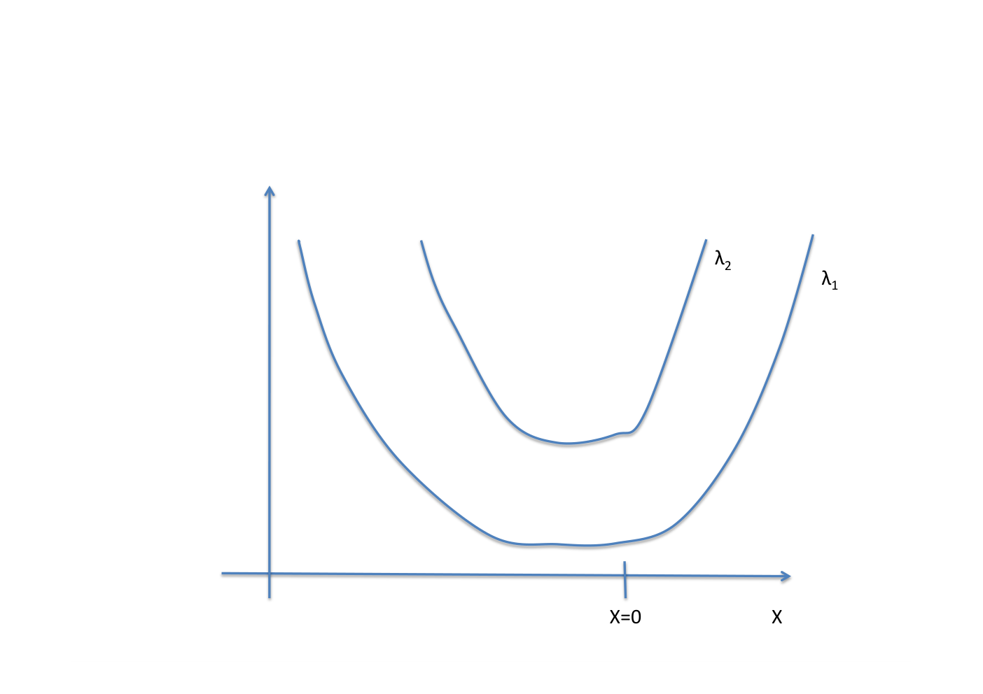
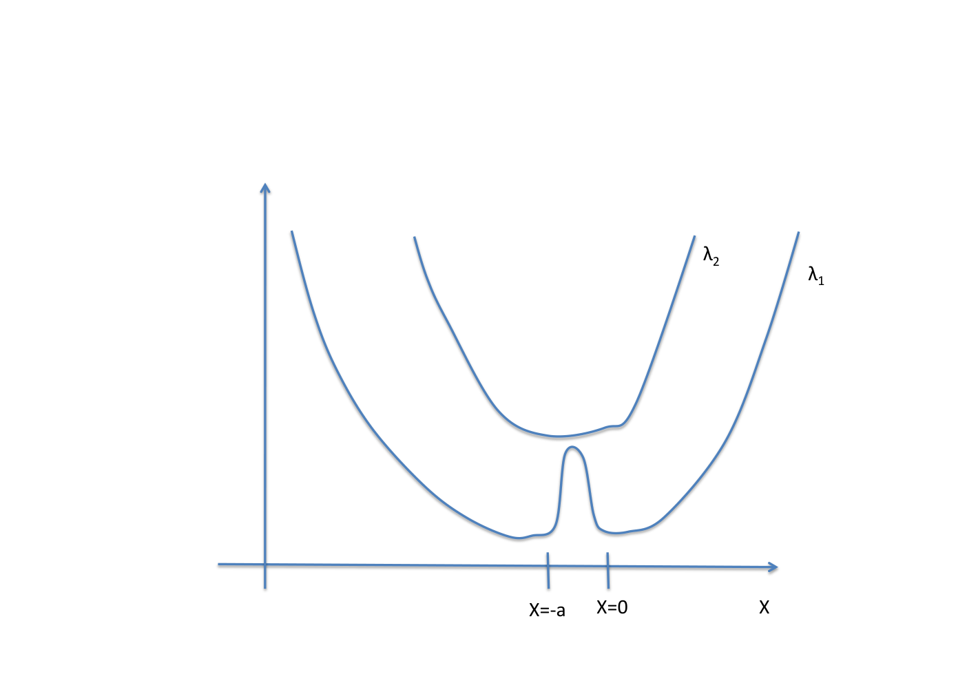
The WKB-method (3.8) shows that
| (3.22) |
are local solutions to the Schrödinger equation (1.2), with positive and negative wave speeds . When the path passes through a domain where the electron eigenvalues are close, the wave function (or ) determined by the transport equation (3.7) yields the probability to transit from the ground state to an excited state, as in the Landau-Zener model (3.9). For a WKB-solution (3.22), with (or ), we can define the transition operator by
| (3.23) |
(and similarly for ) by solving the eikonal and transport equations (3.11) with data given on . The idea is that given the point and the momentum in this point the two first equations determine the path . The third Schrödinger like transport equation in (3.11) then yields a linear solution operator along this path determining at from at . Let us now determine more precisely. We want to determine the global effect of a small transit probability viewed as the perturbation to the eigenvalue problem (3.21) with replacing . To simplify the perturbation analysis we factorize the transition
into a transition between the states and a diagonal matrix , which does not contribute to the transition between states. Since we are only interested in estimates of the small components and , we consider only perturbations generated by the transition matrix . We note that the transition element by (3.23) can be written as the -component of if . Therefore (3.22) shows that the transition element
| (3.24) |
can be determined by the WKB-amplitude function and similarly we have the transition element . The dynamic transition probability , defined by Ehrenfest dynamics in (3.12), measures in this case the amplitude squared in the excited state at for a wave starting in in the ground state. Consequently we have, for and corresponding to the wave speed in (3.22), that
so that by (3.24) , as (namely as the spectral gap becomes large). We assume for simplicity that the transition matrix is translation invariant, so that . The total perturbation becomes the sum of the perturbations of the two WKB-solutions , for the splitting . Hence, we consider perturbations
with the transition from the state to state determined by the matrix component , which is of the (small) order , where , defined in (3.12), is related to the Landau-Zener probability. A reason to decompose the solution into WKB solutions is that their transition is determined by the amplitude functions with approximately conserved norm . The approximate conservation follows from the conservation for the Ehrenfest dynamics (3.15) and the fact that the transport equation (3.7), determining , becomes the Ehrenfest dynamics in the limit .
The perturbed eigenvalue condition becomes
| (3.25) |
where
| (3.26) |
and we want to determine the change in the eigenvector (which measures the probability to be in the excited state) from the perturbed eigenvalue problem (3.25). For this we use the result in the following lemma, whose derivation follows [15].
Lemma 3.3.
Assume that the matrix has distinct eigenvalues, , . Let and be left and and right eigenvectors of , i.e. , , satisfying
For sufficiently small matrices the eigenvectors and eigenvalues of the perturbation matrix are differentiable functions of . If and denote the eigenvector and eigenvalue to that equal the eigenpair to the matrix for , we have that
| (3.27) |
and
| (3.28) |
Proof.
That the eigenvectors and eigenvalues of are differentiable functions of in a neighborhood of follows directly by differentiation of the relations
Let , where is a matrix norm, e.g., the Euclidean operator norm. Let and be the perturbed normalized eigenvector and eigenvalue corresponding to and given by and , and
| (3.29) |
Differentiation of (3.29) at gives
| (3.30) |
Using that and and multiplying by from the left, we get
by the orthogonality between left and right eigenvectors. The Taylor expansion gives (3.27).
The combination of (3.27) in Lemma 3.3 and the assumtion that , as , also when is small, implies that
| (3.31) |
for some positive constant , which determines the perturbation orthogonal to . We will also use that this representation holds separately for each perturbation and . We do not determine the perturbation in the direction, which does not contribute to the transition between states. We denote by the projection of the perturbation on the hyperplane orthogonal to . Since this plane is spanned by the left eigenvectors , we have by (3.27) in Lemma 3.3 that
Returning to the perturbed problem (3.25), we recall from equation (3.19) that the unperturbed eigenvalues are given by
and the corresponding unperturbed eigenvectors are
Lemma 3.3 yields
| (3.32) |
To have the perturbed eigenvalue equal to zero means that we start with an unperturbed eigenvalue in order to obtain the perturbed eigenvalue , satisfying . Using the unperturbed eigenvector , with , yields a perturbation in the component from zero (in the third component of ) to
| (3.33) |
and its squared absolute value measures the probability to be in the excited state, i.e. the probability density , which integrated yields defined in (1.8).
Remark 3.4.
Having a zero eigenvalue of in (3.26) means that the scalar Schrödinger eigenvalue problem
has a solution in the whole domain. We see from (3.33) that when also has a zero eigenvalue we obtain a resonance in the sense that a small perturbation (where ) yields a large change in the eigenvector , meaning that the probability to be in the excited state (which by (3.33) is of the order ) can be of order one even if the perturbation is tiny. Resonance means that the two scalar Schrödinger eigenvalue problems have a coinciding eigenvalue , see Figure 3. An approximation of this probability is
| (3.34) |
3.3.2. Numerical test of the perturbation analysis
A method to numerically test the validity of the perturbation analysis leading to the estimate (3.33), for the one dimensional model, is to compare the probability to be in excited states in (1.8) (determined from numerical approximation of the Schrödinger equation (4.3)) with the expression (3.34) derived from (3.33) in the perturbation analysis. If shows some similarity with (3.34) the perturbation analysis is in some sense justified. The difference , of the eigenvalues in (3.34), can be obtained from numerical approximation of a difference , of the eigenvalues of the decoupled system (3.20), , , using the same centered difference approximation as in (4.3). Let be the set of all eigenvalues, for . By the approximation
where and is chosen such that and are the closest to and using two constants and , we obtain the following estimate of the probability to be in the excited state
| (3.35) |
with being a constant, being an eigenvalue of the discrete two-state Schrödinger equation corresponding to (3.35) and
Conclusions.
Figures 3 and 4 show that the estimation of the probabilities, , to be in the excited state, obtained using the formula (3.35), and the numerically computed probabilities, , to be in the excited state, obtained using the formula (4.4) from the solution of the discrete one dimensional Schrödinger eigenvalue problem (4.3), have similar qualitative behavior in the following two aspects: (1) the minimal value of and are similar, and (2) when is close to a resonance, seen for in (3.35) as , both and become larger. By also adjusting the constant in (3.35) the behavior can also be quantitatively similar, see Figure 3 and 4. That is the perturbation analysis seems to capture this resonance phenomenon, at least qualitatively.
3.3.3. The perturbed eigenvalue problem in the multi-dimensional case
The main idea to extend the one dimensional perturbed eigenvalue problem to multiple dimensions is to write the Schrödinger wave function as a phase-space integral of highly oscillatory functions using the Fourier-Bros-Iagolnitzer transform (FBI-transform). This integral can be viewed as an integral over all hyperplanes in defined in (3.13). Therefore each FBI-mode can be initial data for a WKB solution (3.11) to the right of a hyperplane in and a WKB solution to the left of the hyperplane. The condition to have a differentiable WKB solution across the hyperplane then uses the continuity condition (3.25), as the one dimensional setting, for each point in the hyperplane. The direction of the oscillations in the FBI-mode generates through the WKB-method a molecular dynamics path and an amplitude function. The amplitude function solves, along the path, a transport equation that is well approximated by Ehrenfest dynamics (3.15) and can consequently be computed similarly as the molecular dynamics paths but with smaller time steps, see Sections 3.2 and 4. The integral of WKB-solutions over all hyperplanes contribute through their amplitude functions to the transition, . We will now explain this extension to multiple dimensions more precisely and then in the next section show how to computationally approximate the probability to be in excited states .
We will use the FBI-transform. We could use the standard semi-classical Fourier transform as the initial data for the WKB-method but the FBI-transform has the advantage of giving the high frequency content locally in , i.e. microlocally, which yields a more accurate WKB Ansatz. The important property of the FBI transform
| (3.36) |
is the identity
| (3.37) |
for , where the adjoint operator is defined by
e.g. for all Schwartz functions on , see [25]. Therefore the integral representation
yields suitable boundary data on hyperplanes (e.g. ) for the WKB-method. We will, for each point (in the classically allowed region), use a WKB-function (3.1). In the case of caustics this single WKB-function is replaced by a finite sum of WKB-functions based on the Legendre transform of , as explained in Section 6 and 7,
| (3.38) |
This WKB solution solves the Schrödinger eigenvalue problem (1.2) in the two domains to the left and right of the hyperplane, with the boundary condition constructed so that the WKB-mode is equal to the FBI-mode
for in the hyperplane orthogonal to :
| (3.39) |
The construction of the WKB-solutions in the case of caustics uses asymptotic convergence as , described by the asymptotically equal sign , see [54, 33] and (7.1).
The obtained decomposition
| (3.40) |
determines, for each , the corresponding operators . The total perturbation comes from transitions from all along the paths: for each we let the function solve the transport equation (3.7) along the WKB-path and initialize to the ground state each time is in the hyperplane , generated by . The perturbed wave function is then as in (3.24) determined by
which depends on , by relating in (3.24) with and with in the case of two states. Integrating over all yields the total perturbation, as in (3.26),
at the point . The corresponding perturbed eigenvalue problem (3.25) for the wave function implies, as in (3.33), the following larger change in the excited state
| (3.41) |
at the point , where and depend on . The index in now corresponds to the component in the ground state and the index to be in an excited state, i.e.,
and with the orthogonality conditions
The eigenvalues of the unperturbed problem (3.19) vary highly due the oscillatory functions , with the phase . Figure 4 illustrates a consequence of this variation and indicates that mean values of excitation probabilities corresponding to eigenvalues in a neighborhood are more stable than individual excitations probabilities. Let us therefore consider a local average of the probability to be in the excited state based on a simple model of the smallest eigenvalue (in the excited component) where we assume has a bounded density, , defined on . In the case of one space dimension we can fix a point (in the classically allowed region) where is evaluated, that cuts the spatial domain into two. The average then corresponds to an ensemble of Schrödinger eigenvalues localized around , related to a local mean value of excitation probabilities in Figure 4. We denote this local average by . In higher dimensions we can similarly fix a co-dimension one cutting surface and evaluate on the surface. Let us now study the average excitation probability in this model. Using that yields transition probabilities bounded by one for each as in (3.31) and that outside a compact set (corresponding to the classically allowed region) the factor is negligible small, we have
We conclude that in a model of local ensemble averages of eigenvalues , assuming that for each the eigenvalue difference has a bounded density, then the average probability to be in the excited state has the bound
which, by (3.41) can be written as the average of the square root of the dynamic transition probability
| (3.42) |
3.3.4. Ergodic computation of probabilities to be in excited states
The FBI-transform satisfies
and concentrates on the phase-space set in the limit as and , see [25]. When the dynamics is ergodic, the phase-space measure is in addition uniform on the set as , cf. [37]. The WKB functions behave similarly as locally, since their initial conditions are given by and they solve the Schrödinger equation. We may write where is the momentum for the path at the position that started in the plane given by , since this is a function of and . Therefore we approximate by the following time average of
| (3.43) |
where we used that the transition probability is symmetric by reversing time to . In fact, along a given path also the momentum , at position , is determined by the position and so that is well defined. The relation (3.43) means that we sample square roots, , of transition probabilities along the molecular dynamics path, normalized for each passage through a hyperplane, and then take the average of all hyperplanes. In our computations we sample hyperplanes by means of the phase space trajectory of ground state Born-Oppenheimer molecular dynamics, cf. Algorithm 1 and Figure 5.
4. Numerical examples
The purpose of this section is to present two simple model problems, where the Schrödinger eigenvalue solution can be studied computationally and compared to the molecular dynamics approximation. In the following subsections we
- •
show that the dynamic transition probability in (3.12) can be determined by numerical solution of Ehrenfest dynamics,
- •
verify assumption (2.17) on exponential convergence rate in finite time,
- •
compare numerical approximations of observables from the Schrödinger equation and Born-Oppenheimer molecular dynamics,
- •
compare approximations of the probability to be in excited states from the Schrödinger equation with the molecular dynamics approximation from Algorithm 1.
4.1. Model 1: A one dimensional problem
We consider the one dimensional, time-independent Schrödinger equation (1.2) with the heavy-particle coordinate , two electron states and the Hamiltonian operator, , defined by
| (4.1) |
with the potential operator defined by the matrix
| (4.2) |
where the parameter is a non-negative constant and the function is given by
For each the potential defines the eigenvalue problem with the two eigenvalues and two eigenvectors . The eigenvalues are given by , and and respectively denote the ground and the excited state vector.
Choosing gives a conical intersection at , and a positive value of gives a minimum gap between and at . A small value of corresponds to a large probability to be in excited states and a large value of corresponds to a small probability to be in excited states. Figure 6 illustrates examples of small and large spectral gaps between and with two different values of , respectively.
4.1.1. The 1D discretized Schrödinger equation
We use a central difference method to solve the one dimensional two-state Schrödinger equation (1.2) in the domain with , mesh-size and partition . The approximation of the eigenvalue problem with the eigenvector components and corresponding eigenvalue becomes
| (4.3) |
using homogeneous Dirichlet boundary conditions .
The approximation of the probability to be in the excited state is given by
| (4.4) |
4.1.2. Approximation of the dynamic transition probability
We show in this computational example that the dynamic transition probability, , defined in (3.12), can be obtained from Ehrenfest molecular dynamics simulations (3.15) using the following formula
| (4.5) |
with denoting the time. We observe that numerical experiments illustrate that the transition probability approximates, as time tends to infinity, the Landau-Zener probability as defined in (3.10), given the Landau-Zener model (3.9), see Figure 8.
We approximate the solution of the transport equation (3.7) by the Ehrenfest molecular dynamics simulations (3.15) with (equal to the smallest eigenvalue of in(4.2)) in the Hamiltonian (3.16). For this computational example, we choose , and the initial conditions , , , and . We approximate the solution of the molecular dynamics using the Störmer-Verlet method, [18], based on the two symplectic Euler steps,
| (4.6) |
Conclusions.
Figure 7 illustrates that the potential energy function , obtained from the Ehrenfest molecular dynamics simulations is equal to the ground state energy, , until the dynamics reaches the avoided conical intersection. Then it deviates from the ground state energy and continues in between the ground and excited state energies.
4.2. Model 2: A two dimensional problem
We consider the two dimensional, time-independent Schrödinger equation (1.2) with the heavy-particle coordinate and two electron states . The Hamiltonian is
with
| (4.7) |
where is the identity matrix, the functions are given by (A) or (B) below and , and . As in Example 1, we have for each the eigenvalue problem, , with the eigenvalues and the ground state and excited state eigenvectors and , respectively. We choose the energy, . In this example we study the following two cases of interactions between the two potential surfaces and :
- (A)
A line intersection. We choose and , where is a non-negative constant that defines the minimum distance between the potential surfaces. In this example, the potential surfaces intersect each other (for ) or have the minimum distance between each other at the line . Here, choosing a small value for corresponds to a large probability to be in excited states and a large value for will give a small probability to be in excited states. The parameter in this two dimensional example is analogous to the parameter in the one dimensional example given in Section 4.1.
- (B)
A conical intersection. We choose and with being a chosen point in the two dimensional space. If is chosen such that are smaller than the energy, , we have a conical intersection between the potential surfaces at the point in the classically allowed region , otherwise we have a positive gap between the potential surfaces in the domain . Here, choosing in the origin gives a larger absolute momentum, , at the conical intersection whereas choosing far from the origin will yield a smaller , which yield larger and smaller probabilities to be in excited states, respectively. Figure 9 shows level curves of the eigenvalues, along with example molecular dynamics paths, for varying conical intersection points.
4.2.1. The 2D discretized Schrödinger equation
We use a standard finite difference method to discretize the two dimensional Schrödinger eigenvalue problem (1.2) with mesh-size in both the and directions in the computational domain . The unknown eigenvalue components , with the nodal point for , solve the discrete eigenvalue problem
| (4.8) |
with homogeneous Dirichlet boundary conditions and . We use the solution of the discrete Schrödinger eigenvalue problem to determine the approximate Schrödinger observables
| (4.9) |
with and .
The value of the molecular dynamics observable, , is given by
which, for the two dimensional case, can be written11 1 For a fixed , integration using spherical coordinates in the shell yields the dependence which differentiated with respect to gives (4.10) for and the additional factor for . as
| (4.10) |
when depends only on .


4.2.2. Verification of the ergodic rate condition (2.17).
Figure 10 determines the convergence rate in assumption (2.17) based on numerical approximation of the ergodic projected stochastic dynamics (2.10). The numerical method is given by the steps satisfying
| (4.11) |
where is chosen so that . Here and are all independent taking values with probability . The temperature parameter is . This scheme with phase-space path satisfies the convergence assumptions in [12]22 2 Related to examples (4.15) and (4.7) in [12]. so that , uniformly in . Figure 10 shows that in this case . The maximal Lyapunov constant is determined numerically to and the convergence rate exponent in Theorem 2.1 becomes .
4.2.3. Convergence of observables in 2D
Figures 11 and 12 show that the Schrödinger observables, , are close to the ergodic molecular dynamics observables, . We can compare the numerical results in Figures 11 and 12 with Theorem 2.2 for the case when the probabilities to be in the excited state, , are small, as in Figure 13 for in the conical intersection case. We see in Figures 11 and 12 that the standard deviation of for is roughly times of the standard deviation for , i.e. the numerical results agree roughly with an estimate in the theorem, see Table 1.
| -0.3079 | -0.3159 | |
| -0.3052 | -0.2506 | |
| -0.2744 | -0.2950 | |
| -0.2671 | -0.2890 |
4.2.4. Approximation of the probability to be in excited states
We approximate the probability to be in the excited state, , from the Schödinger equation by the approximation, , from Algorithm 1, using Ehrenfest molecular dynamics simulations based on the Störmer-Verlet method as in (4.6). We choose , , , (line intersection) and (conical intersection).
Conclusions.
Figure 15 shows the probabilities, , to be in the excited state determined from the discrete Schrödinger eigenvalue problem (4.8) based on the formula (4.4). We note that for large gaps, in the right column, the probabilities to be in the excited state, , are either small or close to one, as expected, while for small gaps, in the left column, takes values in the whole interval . We also observe the lack of the structure present in the analogous Figure 4 for the one dimensional case, due to not having the resonances ordered with the eigenvalues as in the one dimensional case discussed in Remark 3.4.
Figure 13 shows determined from the discrete Schrödinger eigenvalue problem and from molecular dynamics simulations for both line and conical intersection cases computed by Algorithm 1. The shapes of the respective methods’ solutions are similar, especially when the probability to be in the exited state, , is small. Figure 14 presents an empirical probability density of inter-arrival hitting times of hyperplanes, cf. Algorithm 1. The empirical density is well approximated by a heavy tailed Burr XII probability density, which indicates that long inter-arrival hitting times are non-negligible. In Figure 16, we observe an expected decay of for the relative error when studying the conical intersection problem with . In the more unstable parameter setting of , however, the error decay is slower with an observed rate of convergence slightly slower than the expected . This might be due to a longer correlation length in the molecular dynamics and hyperplane sampling of Algorithm 1 when the parameter values of are close to .
Remark 4.1.
[Extension to higher dimension] The formation of a conical intersection for a symmetric matrix requires the eigenvalues to be equal, which means that the off diagonal element is zero and the diagonal elements are equal at an intersection point. To have a conical intersection point is therefore generic in dimension two and in higher dimensions the intersection is typically a co-dimension two set. An implementation of the algorithm for computing in higher dimensions and for potentials used in chemistry is future work. The relevant geometry in the multi-dimensional case is the distance to this co-dimension two set, which makes the link to two dimensional case studied here.
5. Regularity and Weyl calculus
This section establishes four lemmas where the last three are used in Theorem 2.1 and 2.2. The first lemma proves the bound (2.15) on derivatives of the solution to (2.13), which verifies that assumption (v) in Theorem 2.1 holds for a case with a near crossing of eigenvalues. The second lemma derives -bounds on Weyl quantized operators obtained from mollified symbols, the third and fourth lemma estimate remainder terms related to the Weyl quantization and establishes the Moyal expansion for the setting used in the proofs of Theorem 2.1 and Theorem 2.2.
We will use equation (2.12) written as the Ito equation
| (5.1) |
for the molecular dynamics path , where is the sample space and assume that the Jacobians and and the higher order derivatives , with for , satisfy the bounds
| (5.2) |
uniformly in (but not in ). Here we use the (Frobenius) norm: assume that then and the notation
Lemma 5.1.
Assume (5.2) and that the near crossing is weak, with non vanishing velocity across the near crossing, namely that
| (5.3) |
for a constant and constants independent of , , and . Then for each multi index there is a constant , independent of , , and , such that
| (5.4) |
Proof.
Remark 5.2 below motives the assumptions. First we study solutions to the linearized Ito equation
where solves (5.1)=(2.12) and the stochastic processes and satisfy for each and some positive number the bound
| (5.5) |
Ito’s formula implies
where by assumption (5.2) we have and by (5.3) there holds . Here . We use , with the arbitrarily small diffusion constant in (2.10), so that the contribution from and are negligible compared to those from and . Gronwall’s inequality shows that
| (5.6) |
which by (5.5) implies
| (5.7) |
provided this holds initially for . Analogously for , we obtain by Hölder’s inequality
so that
| (5.8) |
provided this holds initially for .
The second variation satisfies
We have for that
| (5.9) |
and similarly for , which combined with Ito’s formula and Gronwall’s inequality as above imply
using (5.3), that (5.8) yields and
Also the higher variations satisfy
where the stochastic processes and have the bound (5.5), since following (5.9) we have
and similarly for the higher order derivatives. Therefore (5.7) and (5.8) yield
| (5.10) |
We have by Jensens inequality, for ,
Remark 5.2.
We motivate assumption (5.3) by the behavior for the example of the avoided conical intersection eigenvalues for or discussed in Section 4.2 and (3.14). Although , we assume the near crossing is weak, i.e. that for some constant and a codimension set . Then the exponent in Gronwall’s inequality has the bound
provided the near crossing of potential surfaces is located away from the part of where . Here we assume that the velocity through the avoided crossing domain is bounded from below by . Similarly, an assumption satisfies the last estimate in (5.3).
We will use the -quantization and the notation
for any smooth symbol and the Wigner functions and defined in (2.6).
Lemma 5.3.
Assume that and can be written as and , where , and that and have continuous second derivatives with polynomial growth, i.e. for some and and there is a constant such that and uniformly in , then for every
uniformly in .
Proof.
The proof to estimate the operator norm for a symbol has three steps: to determine a representation of the solution of using the FBI transform , to calculate a Fourier multiplicator applied to using the representation and in the third step to verify that the product of two FBI transformed functions is the convolution of the Wigner function with a Gaussian.
1. We will use that the components of the Wigner function convolved with the Gaussian is the product of the FBI transforms (3.36) of the components and
| (5.11) |
as verified in Step 3 below. Consequently, the diagonal entries are non negative
An -quantization remainder can be related to a remainder in the Wigner quantization (with ) by
where for
which is proved in [32] Remark 2.7.3 and related to the expansion of the exponential in (5.18).
We will introduce the convolution with the Gaussian in the estimate of the remainder using the Taylor expansion of the exponential
where the function is defined by . Here we use the notation . The tensor product property (5.11) of implies the matrix norm estimate
| (5.12) |
using the identity in (3.37) for the FBI transform and the matrix norm (or the less sharp Frobenius norm).
2. We have . The goal is to absorb this exponentially growing pre-factor in .
Consider first the case , then . We have so that
where . The inverse Fourier transform of the pre factor is
so that . The estimate (5.12) implies then in the case
If is uniformly bounded in we have by the two moments and that
and by the properties and we obtain
so that
| (5.13) |
Lemma 5.4.
Assume that is smooth and for each and there is a constant such that , then there is a constant such that
| (5.14) |
If for there is a constant such that , then there is a constant such that
| (5.15) |
Proof.
A proof if this is given e.g. in [54] (Theorem 4.21) and presented here for completeness.
Lemma 5.5.
The composition of two Fourier integral operators, with smooth symbols and in the Schwartz space, has the Weyl symbol
| (5.18) |
The remainder is smooth and if , and the remainder satisfies
| (5.19) |
If and are in the Schwartz space there holds
| (5.20) |
where for and
| (5.21) |
for and
| (5.22) |
and for and
| (5.23) |
Proof.
The proof has five steps. The first step uses the definition of the Weyl quantization to define an integral kernel for the product following Hörmander’s work [22]. The next step formulates the Moyal expansion and identifies the remainder as an average of quantizations (2.7), which proves (5.18). The third step writes the -quantized remainder as a Wigner quantization (with ) and estimates the remainder, using that the product of two FBI transformed functions is the convolution of the Wigner function with a Gaussian. Step 4 proves (5.20) and (5.21). Step 5 proves (5.23).
1. To verify (5.18) we start with the definition of the Weyl operator
The inner product
defines the kernel
| (5.24) |
and the inverse Fourier transform implies
| (5.25) |
Our examples have independent of , i.e. , and the kernel of the composition becomes a multiplication
The definition and (5.25) yields
The final step in Hörmander’s derivation uses the standard Fourier transforms of a Schwartz function and of combined with Fourier transform isometry and Taylor expansion function of the exponential. Here we modify this by identifying the remainder in the Moyal expansion for as an quantization (2.7).
2. We use in this step the Fourier transform in the -direction defined for by
The remainder is based on a Taylor expansion of the exponential function as follows
| (5.26) |
The remainder term can be written
where is smooth since is a Schwartz function. The change of variables and (5.24) shows that kernel of the remainder becomes
We note that the kernel for any symbols in the quantization (2.7) is
for . Consequently we have
| (5.27) |
and the next step shows the final bound
| (5.28) |
3.
It remains to estimate the remainder for in (5.28). Lemma 5.3 and Lemma 5.1 imply that we have
uniformly in , which proves (5.28).
4. The general case of two Fourier integral operators, with smooth symbols in the Schwartz space yields
where
The change of variables replacing has the Jacobian and implies
The same expansion as in (5.26) shows that
based on the representation
The kernel for becomes
and as in (5.27) we obtain
We apply this to the special case where is a Schwartz function. Then we have and for Lemma 5.3 yields as in Step 3 the bound
5. If and the symbol is a smooth product of two convolutions, by (2.29), and tends to zero fast for large . We obtain as in Step 3
6. Appendix: Fourier integral WKB states including caustics
6.1. A preparatory example with the simplest caustic
As an example of a caustic, we study first the simplest example of a fold caustic based on the Airy function which solves
| (6.1) |
The scaled Airy function
solves the Schrödinger equation
| (6.2) |
for any constant . In our context an important property of the Airy function is the fact that it is the inverse Fourier transform of the function
i.e.,
| (6.3) |
In the next section, we will consider a general Schrödinger equation and determine a WKB Fourier integral corresponding to (6.3) for the Airy function; as an introduction to the general case we show how the derive (6.3): by taking the Fourier transform of the ordinary differential equation (6.1)
| (6.4) |
we obtain an ordinary differential equation for the Fourier transform with the solution , for any constant . Then, by differentiation, it is clear that the scaled Airy function solves (6.2). Furthermore, the stationary phase method, cf. Section 7, shows that to the leading order is approximated by
| (6.5) |
and to any order (i.e., for any positive ) when . The behaviour of the Airy function is illustrated in Figure 17.
6.1.1. Molecular dynamics for the Airy function
The eikonal equation corresponding to (6.2) is
with solutions for , which leads to the phase
| (6.6) |
We have the Legendre transform
with the solution . Consequently, we obtain by (6.6) that and
We note that this solution is also obtained from the eikonal equation
which is solved by
Thus we recover the relation for the Legendre transform .
6.2. A general Fourier integral ansatz
In order to treat a more general case with a caustic of the dimension we use the Fourier integral ansatz
| (6.7) |
where
based on the Legendre transform relationships (cf. [11])
If the function is not defined for all , but only for we replace the integral over by integration over using a smooth cut-off function . The cut-off function is zero outside and equal to one in a large part of the interior of . The ansatz (6.7) is inspired by Maslov’s work [33], although it is not the same since our amplitude function depends on but not on .
6.2.1. Making the ansatz for a Schrödinger solution
In this section we construct a solution to the Schrödinger equation from the ansatz (6.7). The constructed solution will be an actual solution and not only an asymptotic solution as in [33]. We consider first the case when the integration is over and then conclude in the Remark 6.2 that the cut-off function can be included in all integrals without changing the property of the Fourier integral ansatz being a solution in the -domain where for some satisfying .
The requirement to be a solution means that there should hold
| (6.8) |
Comparing this expression to the previously discussed case of a single WKB-mode we see that the zero order term is now instead of and that we have instead of . However, the main difference is that the first integral is not zero (only the leading order term of its stationary phase expansion is zero, cf. (7.1)). Therefore, the first integral contributes to the second integral. The goal is now to determine a function satisfying
| (6.9) |
and verify that it is bounded.
Lemma 6.1.
There holds where
Proof.
The function is defined as a solution to the Hamilton-Jacobi (eikonal) equation
| (6.10) |
for all . Consequently, the integral on the left hand side of (6.9) is
Let be any solution to the stationary phase equation and introduce the notation
Then by writing a difference as , identifying a derivative and integrating by parts the integral can be written
Therefore the leading order term in is
Denoting the remainder becomes
hence the function is purely imaginary and small
and
| (6.11) |
The eikonal equation (6.10) and the requirement that in (6.8) then imply that
| (6.12) |
The Hamilton-Jacobi eikonal equation (6.10), in the primal variable with the corresponding dual variable , can be solved locally by the characteristics
| (6.13) |
using the definition
The characteristics give
so that the Schrödinger transport equation becomes, as in (3.7),
| (6.14) |
and for
| (6.15) |
with the complex valued weight function defined by
| (6.16) |
This transport equation is of the same form as the transport equation for a single WKB-mode, with a modification of the weight function .
Differentiation of the second equation in the Hamiltonian system (6.13) implies that the first variation satisfies
which by the Liouville formula (6.18) and the equality
in (6.11) yields the relation,
| (6.17) |
for the constant .
Remark 6.2.
The conclusion in this section holds also when all integrals over in are replaced by integrals with the measure . Then there holds .
6.2.2. Liouville’s formula
7. Appendix: The stationary phase expansion
Consider the phase function and let be any solution to the stationary phase equation . We rewrite the phase function
The relation
defines the function , and its inverse , so that the phase is a quadratic function in . The stationary phase expansion of an integral takes the form, see [54],
| (7.1) |
8. Appendix: An alternative motivation for assumption (2.17)
The double average (2.17) in time and phase-space is in Monte Carlo methods approximated by sampling several paths with random initial points . For a single path one expects convergence rate, in the case of bounded correlation times. Many paths correspond in some sense to longer averaging time for a single path and one may ask how long. This answer is related to how the dynamics maps an initial phase-space neighborhood to . The exponential growth of the first variation , for , implies that an initial domain , on the constant energy hyper-surface , is stretched but mapped to the bounded energy surface . If the dynamics is ergodic the sampling density becomes uniform on this energy hyper-surface, asymptotically in time. Paths that are very close are not acting as independent samples for finite . The assumption (2.17) means that the exponential growth of the first variation measures how small the initial distance, , of the paths can be in order to lead to approximately independent paths after time . The paths that are initially close will after time have a distance of order one. The remaining time this number of paths would act as approximately independent samples (over time ), as tested in Figure 18, and would give the expected decay , if the Lyapunov exponent is positive in only one direction, . If Lyapunov exponents are similar to the maximal, we expect the decay .
Figure 18 tests ergodicity for Born-Oppenheimer molecular dynamics simulations with the potential and the double average over time and initial points in (2.17). The vertical axis shows the sampling error and the horizontal axis shows the number of samples for the symplectic Euler method. The convergence rate for (left figure) and (middle figure) indicate independent sample paths while the closer paths with in (right figure) are not acting independently since the convergence is slower. The maximal Lyapunov exponent is in this case computed to be roughly (the others are ), so that the expansion of the path distance from time zero to time becomes and the approximate convergence rate for indicates that as suggested in the paragraph following (2.17). Here , , , . The ergodic limit is approximated in two different ways: by a single symplectic Euler path to and by the Monte Carlo samples (4.10) to . The dashed line shows .
Acknowledgment
The research was partially supported by the U.S. National Science Foundation under the grant NSF-DMS-0813893, U.S. DOD-ARO Grant Award W911NF-14-1-0247, Swedish Research Council grants 621-2010-5647 and 621-2014-4776 and the Swedish e-Science Research Center. P.P. also thanks KTH and Nordita for their hospitality during his visit when the presented research was initiated.
References
- [1] C. Bayer, H. Hoel, P. Plecháč, A. Szepessy and R. Tempone, How accurate is molecular dynamics?, arXiv:11040953.
- [2] F. A. Berezin and M. A. Shubin, The Schrödinger equation, Kluwer Academic Publishers, 1991.
- [3] J. Bolte and R. Glaser, A semiclassical Egorov theorem and quantum ergodicity for matrix valued operators, Comm. Math. Phys. 247 (2004), 391–419.
- [4] M. Born and R. Oppenheimer, Zur quantentheorie der molekeln, Ann. Physik (1927), no. 84, 4571–484.
- [5] A. Bouzounia and D. Robert, Uniform semiclassical estimates for the propagation of quantum observables, Duke Math. J. 111 (2002), 223–252.
- [6] E. Cances, M. Defranceschi, W. Kutzelnigg, C. LeBris, and Y. Maday, Computational chemistry: a primer, Handbook of Numerical Analysis, vol. X, North-Holland, 2007.
- [7] E. Cances, F. Legoll, and G. Stolz, Theoretical and numerical comparison of some sampling methods for molecular dynamics, Math. Model. Num. Anal. 41 (2007), 351–389.
- [8] G. Ciccotti, T. Lelièvre and E. Vanden-Eijnden, Projection of diffusions on submanifolds: Application to mean force computation, Comm. Pure Appl. Math. 61 (2008), 371–408.
- [9] Dall’ara G.M., Discreteness of the spectrum of Schrödinger operators with non-negative matrix values potentials, arXiv:1402.3177.
- [10] J.-P. Eckmann and R. Sénéor, The Maslov-WKB Method for the (an-)harmonic oscillator, Arch. Rat. Mech. Anal. 61 (1976), 153–173.
- [11] L. C. Evans, Partial differential equation, American Mathematical Society, Providence, RI, 1998.
- [12] E. Faou and T. Lelièvre, Conservative stochastic differential equations: Mathematical and numerical analysis, Math. Comput. 78 (2009), 2047–2074.
- [13] C. Fefferman and L. Seco, Eigenvalues and eigenfunctions of ordinary differential operators, Adv. Math. 95 (1992), 145–305.
- [14] D. Frenkel and B. Smith, Understanding molecular simulation, Academic Press, 2002.
- [15] G. H. Golub and C. F. Van Loan, Matrix Computations, John Hopkins University Press, 1996.
- [16] G.A. Hagedorn, High order corrections to the time-independent Born-Oppenheimer approximation I: Smooth potentials, Ann. Inst. H. Poincaré Sect. A, 47 (1987), 1–16.
- [17] G. A. Hagedorn, High order corrections to the time-independent Born-Oppenheimer approximation II: diatomic Coulomb systems, Comm. Math. Phys. 116 (1988), 23–44.
- [18] E. Hairer, C. Lubich and G. Wanner, Geometric numerical integration illustrated by the Störmer-Verlet method, Acta Numerica 12 (2003), 399–450.
- [19] A. Hassel, Ergodic billiards that are not quantum unique ergodic (with an appendix by A. Hassell and L. Hillairet), Annal. Math. 171 (2010), 605–618.
- [20] B. Helffer, A. Martinez, and D. Robert, Ergodicité et limite semi-classique Comm. Math. Phys. 109 (1987), 313–326.
- [21] F. Hérau and F. Nier, Isotropic hypellipticity and trend to the equilibrium for the Fokker-Planck equation with high degree potential Arch. Rational Mech. Anal. 171 (2004) 151–218.
- [22] L. Hörmander, Weyl calculus of pseudo-differential operators, Comm. Pure Appl. Math. 32 (1979), 359-443.
- [23] H. Jeffreys, On certain approximate solutions of linear differential equations of the second order, Proc. London Math. Soc. 23 (1924), 428–436.
- [24] J. Keller and C. Lasser, Propagation of Quantum Expectations with Husimi Functions, SIAM J. Appl. Math. 73 (2013) 1557-1581.
- [25] M. Klein, A. Martinez, R. Seiler, and X. P. Wang, On the Born-Oppenheimer expansion for polyatomic molecules, Comm. Math. Phys. 143 (1992), 607–639.
- [26] C. Lasser and S. Röblitz, Computing expectations values for molecular quantum dynamics, SIAM J. Sci. Comput. 32 (2010), 1465–1483.
- [27] C. Lasser and S. Teufel, Propagation through conical crossings: an asymptotic semigroup, Comm. Pure Appl. Math. 58 (2005), 1188–1230.
- [28] V. F. Lazutkin, KAM theory and semiclassical approximations to eigenfunctions, With an addendum by A. I. Shnirelʹman. Springer-Verlag, Berlin, 1993.
- [29] C. LeBris, Computational chemistry from the perspective of numerical analysis, Acta Numerica, vol. 14, pp. 363–444, CUP, 2005.
- [30] T. Lelièvre, M. Rousset and G. Stoltz, Free energy computations: A mathematical perspective, Imperial College Press, 2010.
- [31] A. Martinez and V. Sordoni, Twisted pseudodifferential calculus and application to the quantum evolution of molecules, Memoirs Am. Math. Soc., 200 (2009), n. 936.
- [32] A. Martinez, An introduction to semiclassical and microlocal analysis, Springer Verlag, 2002.
- [33] V. P. Maslov and M. V. Fedoriuk, Semi-classical approximation in quantum mechanics, D. Reidel Publishing Company, 1981; based on: V. P. Maslov, Theory of perturbations and asymptotic methods, Moskov. Gos. Univ.. Moscow 1965 (Russian).
- [34] M. Dimassi and J. Sjöstrand, Spectral asymptotics in the semiclassical limit, LMS Lecture Note Series, vol. 268, CUP, 1999.
- [35] G. Panati, H. Spohn, and S. Teufel, Space-adiabatic perturbation theory, Adv. Theor. Math. Phys. 7 (2003), 145–204.
- [36] Rayleigh, On the propagation of waves through a stratified medium, with special reference to the question of reflection, Proc. Roy. Soc. (London) Series A 86 (1912), 207–226.
- [37] M. Reed and B. Simon, Methods of Modern Mathematical Physics, I: Functional Analysis, Academic Press INC., 1980.
- [38] M. Reed and B. Simon, Methods of Modern Mathematical Physics, IV: Analysis of Operators, Academic Press INC., 1980.
- [39] D. Robert, Autour de l’approximation semi-classique, Boston, Birkhäuser, 1987.
- [40] M. Sandberg and A. Szepessy, Convergence rates of symplectic Pontryagin approximations in optimal control theory, Math. Model. Num. Anal. 40 (2006), 149–173.
- [41] L. Schiff, Quantum mechanics, McGraw-Hill, 1968.
- [42] E. Schrödinger, Collected papers on wave mechanics, Blackie and Son, London, 1928.
- [43] A. I. Shnirelʹman, Ergodic properties of eigenfunctions, (Russian) Uspehi Mat. Nauk 29 (1974), 181–182.
- [44] H.-M. Stiepan and S. Teufel, Semiclassical approximations for Hamiltonians with operator-valued symbols, arXiv:1201.4608v3
- [45] A. Szepessy, Langevin molecular dynamics derived from Ehrenfest dynamics, Math. Mod. Meth. Appl. S. 21 (2011), 2289-2334.
- [46] D. J. Tanner, Introduction to quantum mechanics: A time-dependent perspective, University Science Books, 2006.
- [47] E. Teller, The crossing of potential surfaces, J. Phys. Chem. 41 (1937), 109–116.
- [48] S. Teufel, Adiabatic Perturbation Theory in Quantum Dynamics, Springer Lecture Notes in Mathematics, 1821 2003.
- [49] P.F. Tupper, Ergodicity and the Numerical Simulation of Hamiltonian Systems, SIAM J. Appl. Dyn. Syst., 4 (2005), 563–587.
- [50] E. von Schwerin and A. Szepessy, A stochastic phase-field model determined from molecular dynamics, Math. Model. Num. Anal. 44 (2010), 627–646.
- [51] G. A Worth and L. S. Cederbaum, Beyond Born-Oppenheimer: molecular dynamics through a conical intersection, Annu. Rev. Phys. Chem. 55 (2004), 127–158.
- [52] S. Zelditch, Quantum ergodicity and mixing of eigenfunctions, in Françoise, Jean-Pierre; Naber, Gregory L.; Tsun, Tsou Sheung, Encyclopedia of mathematical physics. Vol. 1, 2, 3, 4, 5, Academic Press/Elsevier Science, Oxford, 2006.
- [53] C. Zener, Non-adiabatic crossing of energy levels, Proc. R. Soc. Lond. A 137 (1932), 696–702.
- [54] M. Zworski, Semiclassical Analysis, American Mathematical Society, Providence, RI, 2012.